

Submitted:
24 May 2026
Posted:
26 May 2026
You are already at the latest version
Abstract
Accurate R-peak detection in electrocardiogram (ECG) signals is fundamental for cardiovascular analysis. However, most existing methods address differences in sampling frequency (fs) through signal resampling or transfer learning, which may alter the temporal definition of annotated events. In this study, we propose a fs consistent framework for ECG R-peak detection that avoids both resampling and retraining. The proposed method is based on low-sampling morphological learning combined with physiological temporal constraints (PTC). A lightweight classifier (Extreme Gradient Boosting) is trained on 128 Hz ECG data (MIT-BIH Normal Sinus Rhythm Database, XGB) to learn local morphological structures, and feature extraction is defined in milliseconds with time-normalized derivatives to ensure consistency across fs. The trained model is directly applied to higher- fs datasets (360 Hz, 500 Hz, and 1000 Hz) without modification. Final peak locations are determined through deterministic processing, including PTC and local snap processing. Experimental results demonstrated that the proposed method achieved stable detection performance across multiple sampling frequencies. When evaluated in a sample-wise manner, the proposed method achieved mean F1-scores of 0.885 on MIT-BIH Arrhythmia Database (360 Hz), 0.848 on Lobachevsky University Electrocardiography Database (LUDB, 500 Hz, sinus rhythm), 0.837 on LUDB (500 Hz, arrhythmia), and 0.953 on PTB Diagnostic ECG Database (1000 Hz), without any resampling or retraining. The integration of probabilistic candidate detection and deterministic temporal alignment enables consistent peak localization under cross-frequency conditions. These findings demonstrate that augmenting machine learning with deterministic decision mechanisms provides a principled framework for fs -consistent ECG peak detection.
Keywords:
ECG
; R-peak detection
; cross-frequency analysis
; sampling-frequency consistency
; physiological temporal constraints
; morphological learning
1. Introduction
Electrocardiogram (ECG) R-peak detection is a fundamental task in cardiovascular signal analysis and serves as the basis for heart rate variability (HRV) assessment, arrhythmia monitoring, and wearable health systems [1,2]. In recent years, convolutional neural networks (CNNs) and other deep learning (DL) architectures have demonstrated high classification performance in large-scale ECG classification tasks [3,4,5]. Several studies have attempted to address variations in sampling frequency (fs) by incorporating multi-resolution inputs, signal resampling strategies, or transfer learning across datasets [6,7,8,9].
Despite these advances, most cross-dataset approaches rely on modifying either the signal representation or model parameters according to changes in fs [10]. While such strategies may improve empirical detection performance, they implicitly alter the discrete-time structure of annotated events. Resampling changes the temporal grid on which peaks are defined, and transfer learning introduces frequency-specific information into the learned decision boundaries. In this sense, many existing methods achieve frequency adaptation rather than consistent performance across different sampling frequencies.
From the perspective of structural signal processing, waveforms acquired at higher sampling frequencies inherently contain the information represented at lower sampling frequencies. As shown in Figure 1, an ECG signal sampled at a higher frequency provides a denser representation of the same underlying waveform observed at a lower fs. The fs determines the density of observation but does not alter the underlying electrical activity of the heart. The morphological composition of the waveform—its structural organization in the time domain—remains fundamentally unchanged, with higher sampling frequencies providing only a more finely discretized representation. Therefore, if detection is based on temporal features defined in absolute time rather than sample-based features, consistent performance across different sampling frequencies can be achieved in principle without modifying the signal or the model.
Conventional ECG analysis relies on features defined in discrete sample units, which depend on the fs. However, cardiovascular signals arise from continuous physiological processes structured in absolute time. In this study, features are represented in physical time units rather than sample indices. For example, a temporal pattern corresponding to a 30 ms interval learned at 128 Hz can be consistently interpreted as the same 30 ms interval at 1000 Hz. This time-normalized representation reduces dependency on fs and enables consistent extraction of temporal structures across different acquisition settings. This perspective motivates the proposed framework, in which morphological learning captures the underlying “skeleton” of ECG waveforms in the time domain, enabling consistent interpretation across different sampling frequencies.
Based on this perspective, we adopt a design philosophy that deliberately avoids both resampling and retraining. Temporal features are normalized in the time domain, and derivative-based features are scaled according to the fs. This enables the model to operate within a temporally consistent framework across signals sampled at 128 Hz, 360 Hz, 500 Hz, and 1000 Hz. In this study, a lightweight binary classifier is trained using low- fs data. Under the assumption that the skeletal structure of ECG waveforms is invariant across sampling frequencies, the classifier learns local morphological features around R-peak locations as discretized representations of this underlying structure. The trained model is then directly applied to higher- fs signals. Since higher-resolution waveforms can be interpreted as temporally denser representations of the same morphology, the learned features are expected to remain consistent as long as the time scale is preserved. Accordingly, the framework is designed to maintain temporal consistency of annotated peak locations by using time-based representations rather than discrete index intervals.
In our previous work, we introduced a physiology-aware detection framework based on physiological temporal constraints (PTC), in which probabilistic scoring and deterministic decision-making were explicitly separated [11]. In this architecture, a lightweight binary classifier was used solely to estimate candidate likelihoods, while the final R-peak localization was governed by physiologically interpretable temporal constraints and rule-based local refinement. By assigning the decision authority to temporally meaningful rules rather than the classifier itself, the framework improved robustness to class imbalance, reduced sample-wise false positives, and enhanced interpretability. However, the temporal behavior of this structurally decoupled framework under strict cross-frequency conditions has not yet been systematically investigated.
In this study, we evaluate ECG R-peak detection across multiple sampling frequencies without resampling or transfer learning. A model trained on low- fs data is directly applied to higher- fs signals while preserving the principles of temporal normalization and the separation of probabilistic scoring and deterministic control. Through cross-frequency experiments and distribution-based temporal error analysis, we characterize the temporal localization behavior independently of classification performance and present a structural framework for fs -invariant peak detection.
2. Materials and Methods
2.1. Morphological Skeleton Learning
In this study, morphological learning refers to the extraction and modeling of local waveform structures that characterize the shape of ECG signals in the time domain. Rather than learning sampling-specific discrete patterns or absolute amplitude values, the model is designed to capture essential morphological features that represent the underlying structure of the waveform.
Importantly, the use of low- fs ECG data does not constrain the model to sampling-specific representations. Instead, it encourages the learning of fundamental morphological structures that can be consistently interpreted across different sampling frequencies. In this sense, the learned representation can be regarded as a coarse “skeleton” of the ECG waveform, preserving its essential shape while remaining robust to variations in sampling density.
By defining feature extraction in milliseconds and normalizing time-dependent features, the proposed framework ensures that these morphological representations remain consistent across signals sampled at different frequencies. As a result, the model can generalize from low- fs data to higher-resolution signals without modification.
An overview of the proposed ECG R-peak detection framework is illustrated in Figure 2. The framework consists of two main stages: probabilistic scoring and deterministic decision-making. The probabilistic stage employs a lightweight classifier to estimate sample-wise likelihoods of R-peak candidates. The deterministic stage integrates PTC, including a refractory period constraint and a sequential selection process, with local snap processing (LSP) for temporal alignment. The final R-peak locations are determined through this rule-based decision and correction process.
Within this framework, Section 2.1 describes the construction and training of the morphological skeleton learning model used for coarse R-peak candidate detection. The classifier is designed to learn a coarse morphological representation (skeleton) of ECG waveforms rather than precise peak locations. This design enables the model to capture fundamental waveform structures that can be consistently interpreted across different sampling frequencies.
The following subsections first define the feature representation used for morphological skeleton learning and then describe the training and evaluation procedures. The robustness and generalization performance of the learned model are subsequently assessed, followed by cross-frequency evaluation under varying sampling conditions.
2.1.1. Feature Normalization for Cross-Frequency ECG Peak Detection
The feature set used in this study was derived from the ECG peak detection framework proposed in our previous work [11]. In that framework, eleven lightweight morphological features were defined and grouped into four categories: (a) amplitude and statistical features, (b) differential and curvature features, (c) slope and energy-based features, and (d) direct amplitude information, as summarized in Table 1.
In this study, the feature extraction window was defined in the time domain using a window length win_ms (in milliseconds). The corresponding number of samples was determined based on the fs in order to preserve the temporal interpretation of the features across datasets. Formally, the half-window size h was defined as:
where round(x) denotes rounding to the nearest integer, and the total window length was given by:
ensuring an odd number of samples with a well-defined center.
For each central sample , a symmetric local window
was extracted from the ECG signal, and 11 lightweight morphological features were computed. These features were designed to capture local waveform characteristics common to P, R, and T waves while keeping the computational cost low. At the signal boundaries, complete windows could not be formed; therefore, samples within ±h points from the edges were excluded from the analysis.
where for denotes the relative sample index within the local window, and denotes the ECG amplitude at index . and represent the mean values of and , respectively. denotes the window length.
In the previous framework, ECG signals were sampled at 500 Hz, and the window length was implemented as a fixed number of samples corresponding to a specified temporal duration. However, when the fs differs across datasets, the number of samples corresponding to the same temporal window must be adjusted to preserve the temporal interpretation of the features. In our previous framework (500 Hz), a temporal window of approximately 30 ms yielded the best performance. This value was adopted as a time-domain reference and adjusted to 32 ms to maintain consistency under 128 Hz sampling. In addition, neighboring window lengths (16 ms and 48 ms) were considered to assess robustness to variations in temporal scale.
In this study, the window length was defined in milliseconds, and the corresponding number of samples was determined based on the fs. According to the above definition, the corresponding number of samples can be calculated by converting the temporal window length into sample counts based on the fs. For example, for a window length of 32 ms, the corresponding total window length was 5 samples at 128 Hz, 13 samples at 360 Hz, 17 samples at 500 Hz, and 33 samples at 1000 Hz, according to Eqs. (1) and (2). In all cases, an odd number of samples was used to ensure that each sliding window has a well-defined center sample.
Although this adjustment preserves the temporal extent of the feature extraction region, several features inherently depend on the sampling interval and therefore require additional normalization. In particular, first-order derivatives, second-order derivatives, and slope-related features are sensitive to the fs. These features explicitly involve temporal differences between adjacent samples. Therefore, their values vary depending on the sampling interval, even when the underlying waveform morphology is identical.
To ensure comparability across sampling frequencies, these features were normalized with respect to time and expressed per millisecond. Specifically, the normalization was applied as follows:
where Δt denotes the sampling interval (Δt = 1/fs). In the previous framework, the slope feature was defined using the sample index , making it implicitly dependent on fs. In the present study, this definition was reformulated in the time domain by replacing the sample index with the corresponding time coordinate, allowing the slope to be interpreted as a temporal rate of amplitude change (V/s). Similarly, the difference energy featurewas reformulated to incorporate Δt by calculating the mean of (Δw/Δt)2, which can be expressed as follows:
This ensures thatrepresents the energy of the signal’s derivative in physical units (V2/s2). By defining these features in the time domain, their numerical scales remain consistent across diverse sampling frequencies, which is fundamental to the cross-frequency robustness of the proposed framework.
To train the classifier responsible for coarse R-peak candidate detection, ECG data from the MIT-BIH Normal Sinus Rhythm Database (MIT-NSRDB) were used [12]. The selection of low- fs ECG data was intentional. The MIT-NSRDB consists of long-term ECG recordings from subjects with stable sinus rhythm, sampled at 128 Hz.
The dataset comprises 18 subjects, including 5 males (36 ± 7 years, range: 26–45) and 13 females (34 ± 9 years, range: 20–50). Each record contains approximately 24 hours of Lead II ECG data. Upon verification of the actual recording durations, the average recording length was 24.2 ± 0.8 hours. These long-term sinus rhythm recordings provide stable waveform segments suitable for learning the fundamental morphological structure of the QRS complex (QRS).
Inspection of the annotated R-wave labels revealed that the annotations were assigned not at the R-peak locations but rather to a location roughly between the Q-wave and the R-wave, as illustrated in Figure 3. However, in the proposed peak detection framework, the role of machine learning is not to determine the exact peak position, but rather to provide auxiliary scoring for identifying candidate peaks or regions near the peaks. Therefore, the presence of labels in the vicinity of the peak is sufficient for training.
On the other hand, the data volume of each record is extremely large. The number of samples per record is given by 24 h × 3600 s × 128 Hz = 11,059,200 samples. To reduce computational cost, a subsampling strategy was adopted in which 2-minute segments were extracted at 8-minute intervals. As a result, 2,211,840 samples were used from each record, corresponding to approximately 288 minutes (4.8 hours) of data.
For preprocessing, a low-pass filter (LPF) with a cutoff frequency of 40 Hz was first applied to remove high-frequency noise and spike artifacts. This was followed by a high-pass filter (HPF) with a cutoff frequency of 0.1 Hz to eliminate baseline drift. Subsequently, as in the previous study [11], each record was segmented into 10-second intervals, and z-score normalization was applied to each segment such that the mean and standard deviation (SD) were set to 0 and 1, respectively.
2.1.2. Robustness Evaluation of Morphological Skeleton Learning
To evaluate the accuracy and robustness of morphological skeleton learning in the proposed framework, a record-level six-fold cross-validation (k = 6) scheme was employed. The data were partitioned based on a predefined record-level split, where each fold consisted of 12 records for training, 3 records for validation, and 3 records for testing. Care was taken to ensure that the same ECG record was not included in multiple subsets, thereby preventing data leakage. The detailed record allocation for each fold is provided in Table S1 (Supplementary Materials).
As the classifier, Extreme Gradient Boosting (XGB), which demonstrated the most stable performance in our previous study, was adopted. In the previous framework, a lightweight classifier was used to generate likelihood scores of peak candidates based on local morphological features, while the final peak determination was governed by PTC. In this study, this concept was applied to morphological skeleton learning for R-peak detection, where samples near the rising edge of the R-wave, rather than the peak itself, were treated as positive instances in a binary classification task against background samples.
The feature set consisted of the eleven local morphological features defined in the previous section. The feature extraction window length (win_len) was evaluated under three conditions: 16 ms, 32 ms, and 48 ms. The central value of 32 ms was selected based on our previous study, in which a window length of approximately 30 ms yielded optimal performance at 500 Hz. In the present study, this value was adopted as a time-domain reference and adjusted to 32 ms to maintain consistency under 128 Hz sampling. The additional conditions (16 ms and 48 ms) were included to evaluate robustness around this reference scale. For XGB, the following hyperparameters were considered:
number of estimators: n_estimators ∈ {200, 300}
maximum tree depth: max_depth ∈ {3, 4}
learning rate: learning_rate ∈ {0.05, 0.1}
The optimal combination was selected based on the highest sample-level F1-score (F1) on the validation set. The classification threshold was fixed at 0.5. Due to the severe class imbalance between positive and background samples, the scale_pos_weight parameter was computed based on the label distribution in the training data. After determining the optimal hyperparameters, the classifier was retrained using the combined training and validation datasets.
Subsequently, as a second-stage optimization, the PTC-related parameters for R-peak candidate selection—namely, the decision threshold (θR) and refractory period (refR) were optimized via grid search on the validation set. The search ranges were defined as:
θR ∈ {0.40, 0.45, 0.50, 0.55, 0.60, 0.65, 0.70, 0.75, 0.80, 0.85, 0.90, 0.95, 1.00}
refR ∈ {30, 40, 50, 60, 70, 80} ms
In this second stage, candidate points near the R-wave were extracted based on the classification scores, and a sequence of candidates was constructed through sequential selection with a refractory constraint. The detected peaks were then matched to annotation labels using a one-to-one correspondence within a tolerance window of ±20 ms, and the sample-wise F1 was computed. Finally, the θR and refR that maximized the sample-wise F1 were selected as the optimal detection parameters for each fold.
To interpret the contribution of each feature in the trained classifier, feature importance was evaluated using the XGB built-in scoring functions. Two importance metrics were considered: gain and weight. The gain represents the average improvement in the loss function brought by a feature when it is used for splitting, while the weight indicates the number of times a feature is used in tree splits. This analysis was used to qualitatively assess which morphological features contributed most to candidate detection.
2.1.3. Fixed-Split Validation of the Morphological Skeleton Learning Classifier
In Section 2.1.2, the robustness of morphological skeleton learning in the proposed framework was evaluated using six-fold cross-validation. In addition to this, the stability of the classifier was further assessed using a fixed record-level split of the NSRDB dataset. Specifically, the 18 records were divided into 14 records for training and 4 records for validation (Table 2). The partitioning was performed at the subject level to ensure that the same ECG record was not included in multiple subsets, thereby preventing data leakage.
The classifier, feature set, and hyperparameter optimization procedure were identical to those described in Section 2.1.2. The purpose of this section is to verify that the proposed method maintains stable performance on unseen records under a fixed data partition, independent of cross-validation. As shown in Table 2, the training and validation datasets were separated at the record level to prevent data leakage between subsets.
Although the number of records in the NSRDB is limited, each record contains approximately 24 hours of ECG data, resulting in a large number of temporally diverse waveform segments for morphology learning. Because both the training and validation sets were derived from stable sinus-rhythm recordings within the same database, this evaluation primarily reflects the internal stability of morphology-based candidate detection under homogeneous conditions rather than true cross-dataset generalization.
2.2. Cross-Frequency Evaluation
To evaluate cross-frequency robustness, the model trained at 128 Hz was tested on ECG datasets recorded at different sampling frequencies.
2.2.1. ECG Datasets
For cross-frequency evaluation, three publicly available ECG datasets were used:
(a) MIT-BIH Arrhythmia Database (MIT-AD)
The MIT-AD contains 48 half-hour two-channel ECG recordings obtained from 47 subjects [13]. The signals were sampled at 360 Hz. In this study, since morphological skeleton learning was performed using only Lead II, 46 records with available Lead II signals were included in the analysis (male: 64 ± 21 years, n = 26; female: 62 ± 23 years, n = 20; age unknown for 2 records). Each record has a duration of 30 minutes and 6 seconds. Reference annotations indicate the R-peak locations.
(b) Lobachevsky University Electrocardiography Database (LUDB)
The LUDB consists of ECG recordings from 200 subjects and was analyzed separately for sinus rhythm records (male: 49 ± 18 years, n = 77; female: 55 ± 19 years, n = 65) and arrhythmia records (male: 53 ± 21 years, n = 38; female: 52 ± 21 years, n = 20) [14,15,16]. The ECG signals were sampled at 500 Hz, and each record has a duration of 10 seconds. Among the 12 leads, only the Lead II signal was used. Reference R-peak annotations were based on expert-annotated labels provided in the dataset.
(c) PTB Diagnostic ECG Database (PTB)
The PTB database contains 549 ECG recordings obtained from 290 subjects [17]. Each recording includes 15 simultaneously measured channels consisting of 12 standard leads and 3 Frank leads (vx, vy, vz). The signals were sampled at 1000 Hz, and each record has a duration of approximately 120 seconds. In this study, 80 records corresponding to 52 healthy control subjects were extracted for analysis (male: 42 ± 14 years, n = 39; female: 48 ± 18 years, n = 13). Only the Lead II signal was used. Reference R-peak annotations are not available for this dataset.
2.2.2. LSP for Peak Alignment
The proposed morphology-based classifier learns samples around the rising edge of the R-wave as positive instances, which leads to systematic temporal bias in detected peak locations. To correct this discrepancy with respect to the true R-peak position, a LSP method was introduced. For each detected peak candidate at time t0, a search window of width Δsnap was defined, and the sample with the maximum ECG amplitude within this window was selected as the corrected peak location:
where x(t) represents the preprocessed ECG signal after bandpass filtering and normalization, and Δsnap denotes the search window width. This process reduces variability in peak localization caused by differences in detection algorithms, sampling frequencies, and annotation definitions. The search window width Δsnap was determined based on the empirical distribution of detection errors (detected time − reference time) prior to LSP. Specifically, Δsnap was set to approximately three times the SD of the error distribution, covering the majority of observed deviations. Based on this criterion, Δsnap was fixed at 20 ms in this study.
2.2.3. Multi-Detector-Based R-Peak Candidate Generation for Silver-Standard Construction
To construct Silver-standard annotations for the PTB dataset, a multi-detector framework integrating two complementary R-peak detectors was employed. ECG signals were first preprocessed using a bandpass filter (0.4–40 Hz, 2nd-order Butterworth) to stabilize detection while preserving QRS morphology. Two independent R-peak detectors were then applied to the preprocessed signals.
The first detector was based on the NeuroKit2 implementation [18] of a Pan–Tompkins-type algorithm [2], which emphasizes steep QRS upslopes through differentiation and integration, enabling gradient-based peak detection. The second detector was the gqrs algorithm implemented in the WFDB Python package (PhysioNet) [16], a well-established QRS detection method based on adaptive thresholding, QRS width estimation, and refractory period control.
To reduce variability in peak localization across detectors, LSP, as defined in Section 2.2.2, was applied to the outputs of each detector prior to integration. Specifically, detected peak positions were aligned to the nearest local maximum within a ±30 ms window. This tolerance window was defined to account for temporal variability in detector outputs while preserving physiologically plausible alignment.
The aligned peak candidates from both detectors were then integrated using a detector-agreement strategy. Peaks detected by both methods within a temporal tolerance window of ±8 ms were grouped into clusters, and only clusters supported by both detectors were retained. The representative peak position for each cluster was defined as the median of the detected sample indices, ensuring robustness against minor discrepancies between detectors.
Finally, the merged peak positions were refined by applying LSP again using the same ±30 ms window, ensuring precise alignment with the local maxima of the ECG signal. Duplicate peaks were removed to obtain a unique set of R-peak candidates.
The resulting peak set was used as Silver-standard annotations, where each detected R-peak was assigned a label value of 1, and all other samples were labeled as 0. The overall procedure is summarized in Algorithm 1.
Algorithm 1: Multi-detector-based Silver-standard construction
Input: ECG signal x_raw, fs
Output: Silver-standard R-peak set R_silver
1: x ← bandpass_filter (x_raw)
2: R_NK ← NeuroKit (x, fs)
3: R_GQRS ← gqrs(x, fs)
4: R_NK ← LSP (R_NK, x, fs, 30 ms)
5: R_GQRS ← LSP(R_GQRS, x, fs, 30 ms)
6: R_merge ← detector_agreement (R_NK, R_GQRS, 8 ms)
7: R_silver ← LSP (R_merge, x, fs, 30 ms)
8: R_silver ← unique (R_silver)
9: return R_silver
An example of the Silver-standard R-peak annotations in the PTB dataset is shown in Figure 4. The detected peaks are aligned with the local maxima of the ECG waveform after LSP, demonstrating the consistency of the annotation process. During the Silver-standard construction process, four records (patient180/s0476_re, patient239/s0467_re, patient267/s0504_re, and patient279/s0533_re) showed inconsistent R-peak detections between the two detectors (NeuroKit and gqrs) and were excluded from further analysis. As a result, a total of 76 PTB records were used in this study.
2.2.4. Filtering Conditions
To isolate the effect of frequency components, only the cutoff frequencies of the filters were varied during testing, while the XGB parameters and PTC-related parameters were fixed to the optimal values determined in Section 2.1.2. In addition to the default filtering condition, the cutoff frequency of the LPF was varied at 10, 20, and 30 Hz, and the cutoff frequency of the HPF was varied at 0.05, 0.2, 0.3, and 0.4 Hz. After filtering, each record was segmented into 10-second intervals. For each segment, z-score normalization was applied such that the mean and SD were set to 0 and 1, respectively.
2.2.5. Performance Metrics
Sample-wise classification performance was evaluated using sensitivity (Se), positive predictive value (PPV), and F1, computed based on sample-wise comparisons between predicted labels and reference annotations. These metrics are defined as:
where TP, FP, and FN denote the number of true positive, false positive, and false negative samples, respectively. For temporal evaluation, detected peak locations were compared with reference annotations using a tolerance window of ±20 ms. The corresponding detection results were summarized using the number of TP, FP, and FN.
Results are reported as mean ± SD across records. All experiments were conducted with and without LSP, allowing direct comparison of its contribution to cross-frequency robustness.
All analyses and evaluations were implemented in Python 3.12.7 (64-bit). Numerical computation and data handling were performed using NumPy and Pandas. ECG preprocessing was conducted using a bandpass filter implemented with the Butterworth filter and zero-phase filtering (filtfilt) functions from SciPy. R-peak detection was performed using the NeuroKit and WFDB toolkits. Machine learning models were implemented using scikit-learn, with XGB employed as the classifier.
3. Results
The morphological skeleton learning model described in Section 2.1 was trained using MIT-NSRDB sampled at 128 Hz, and its performance under this training condition is first presented below. Table 3 summarizes the sample-wise R-peak detection performance across six folds for three different temporal window lengths (16 ms, 32 ms, and 48 ms). Performance was evaluated using Se, PPV, and F1, with a matching tolerance of ±20 ms. Across all window lengths, the proposed method achieved high and stable performance, with mean F1 ranging from 0.935 to 0.948. The differences in performance between window lengths were small, indicating that the method is robust to the choice of temporal window duration when defined in milliseconds. Specifically, the 16 ms, 32 ms, and 48 ms windows yielded F1 of 0.946 ± 0.059, 0.935 ± 0.073, and 0.948 ± 0.057, respectively. Although the 32 ms configuration exhibited slightly higher variability, all three settings demonstrated comparable detection accuracy.
Table 4 summarizes the validation results obtained using the fixed record-level split of the MIT-NSRDB dataset. Detection performance was evaluated using Se, PPV, and F1 with a matching tolerance of ±20 ms. Across all window lengths, the proposed method demonstrated highly stable detection performance, with F1 consistently around 0.998. The differences between window lengths were minimal, indicating that the morphology-based candidate detection framework is largely robust to temporal window duration when defined in milliseconds.
The optimal decision parameters were also stable across window lengths. The decision threshold θR converged to 0.90–0.95, while the refractory period refR ranged from 40 to 80 ms, which is consistent with physiologically plausible R–R interval constraints. Among the evaluated configurations, the 32 ms window yielded the highest validation F1 and was selected as the final implementation configuration for subsequent cross-frequency evaluation.
Because both the training and validation sets were derived from stable sinus-rhythm recordings within the same database, the results shown in Table 4 should be interpreted primarily as an evaluation of the internal stability of morphology-based candidate detection under homogeneous recording conditions.
The optimal parameter set of the implementation model is summarized in Table 5. These parameters were determined based on the highest validation F1 obtained at MIT-NSRDB and were fixed for all subsequent cross-frequency evaluations. The selected parameters were consistent across preprocessing, classifier, and decision control components. The low-pass and high-pass cutoff frequencies were set to 40 Hz and 0.1 Hz, respectively. The PTC-related parameters converged to a decision θR of 0.9 and a refR of 80 ms, which are physiologically plausible values for R-peak detection. The optimal temporal window length was 32 ms, providing a balance between temporal resolution and feature stability. For the XGB classifier, the number of estimators, maximum depth, and learning rate were set to 300, 4, and 0.1, respectively.
Table 6 summarizes the feature importance of the trained XGB classifier in terms of both gain and weight. Gain (%) represents the relative contribution of each feature to loss reduction, while weight indicates the number of times the feature is used for splitting. In terms of gain, the maximum amplitude (max) showed the highest contribution (72.3%), followed by std (13.3%) and energy (8.9%). All other features contributed less than 2%. In terms of weight, the first-order derivative (d1) was the most frequently used feature for splitting (602), followed by energy (500), minimum value (496), and slope (438).
Cross-frequency R-peak detection performance with and without LSP is summarized in Table 7. Unless otherwise specified, the default bandpass filtering condition was defined as a low-pass cutoff of 40 Hz and a high-pass cutoff of 0.1 Hz. When the LPF cutoff was set to 10 Hz, the HPF cutoff was fixed at 0.1 Hz. Conversely, when the HPF cutoff was set to 0.4 Hz, the LPF cutoff was fixed at 40 Hz. Detailed results for intermediate filtering conditions (LPF = 20–30 Hz and HPF = 0.2–0.3 Hz) are provided in Table S2 (Supplementary Materials).
On the MIT-AD, higher performance was obtained with LSP across most filtering conditions. Under the default condition, the mean F1 increased from 0.615 ± 0.358 (without LSP) to 0.878 ± 0.208 (with LSP), while the highest performance (F1 = 0.885 ± 0.206) was obtained under HPF = 0.4 Hz. Under LPF = 10 Hz, performance decreased substantially in both cases.
In the LUDB sinus rhythm subset (500 Hz), F1 with LSP were higher than those without LSP under all evaluated conditions. Under the default condition, F1 increased from 0.755 ± 0.255 to 0.820 ± 0.181, while the highest value (F1 = 0.848 ± 0.136) was observed under HPF = 0.4 Hz.
In the LUDB arrhythmia subset (500 Hz), higher F1 were consistently obtained with LSP. Under the default condition, F1 increased from 0.705 ± 0.277 to 0.808 ± 0.178, while the highest performance (F1 = 0.837 ± 0.138) was again obtained under HPF = 0.4 Hz. Performance decreased under LPF = 10 Hz for both conditions.
In the PTB (1000 Hz), LSP also resulted in higher performance. Under the default condition, F1 increased from 0.876 ± 0.204 to 0.935 ± 0.129, while the highest performance (F1 = 0.953 ± 0.143) was obtained under HPF = 0.4 Hz. Across all datasets, LPF = 10 Hz consistently degraded performance.
Table 8 summarizes the temporal localization error of detected R-peaks with and without LSP across all datasets. The error was defined as the time difference between detected and reference R-peak locations (detected − reference).
Without LSP, a negative mean error was consistently observed across all datasets. The mean error was −14.5 ± 7.0 ms for MIT-AD, −13.1 ± 6.1 ms for LUDB sinus rhythm, −13.0 ± 7.0 ms for LUDB arrhythmia, and −13.9 ± 7.3 ms for PTB.
With LSP, the mean error was reduced in all datasets. The mean error changed to −1.3 ± 4.4 ms for MIT, 1.4 ± 2.5 ms for LUDB sinus rhythm, 1.4 ± 3.4 ms for LUDB arrhythmia, and −0.6 ± 3.0 ms for PTB. In addition, the SD decreased after applying LSP in all datasets, indicating reduced variability in temporal localization.
To visually illustrate the effect of LSP on temporal alignment, representative examples of R-peak detection results with and without LSP are shown in Figure 5, Figure 6, Figure 7 and Figure 8 for different datasets and sampling frequencies. The ECG signals shown in these figures correspond to the preprocessed signals after bandpass filtering, as described in Section 2. In all cases, detections without LSP are located earlier than the reference peak positions. After applying LSP, the detected peaks are positioned closer to the local maxima of the ECG waveform. These visual results are consistent with the quantitative error values presented in Table 8, where the negative mean error observed without LSP is reduced after correction.
4. Discussion
4.1. Cross-Frequency Robustness of the Proposed Framework
The present study investigated ECG R-peak detection under cross-frequency conditions without resampling or transfer learning. A classifier trained on low- fs ECG data (128 Hz) was directly applied to higher- fs datasets (360 Hz, 500 Hz, and 1000 Hz), while maintaining temporal consistency through time-domain feature normalization and a structurally decoupled detection framework.
The results demonstrated that the proposed framework achieved stable detection performance across different sampling frequencies. In particular, sample-wise F1 were consistently maintained, indicating that the learned morphological representation can be applied across signals with different temporal resolutions.
4.2. Systematic Temporal Bias and Its Origin
A key finding of this study is that morphological learning based on low- fs ECG signals can be effectively transferred to high- fs signals without resampling or retraining. This result supports the underlying assumption that high- fs ECG waveforms contain the same fundamental morphological structures as their low- fs counterparts, and that these structures can be captured through time-domain feature representations, as suggested in previous studies on time-scale consistency in physiological signals [19,20].
Another important observation is the systematic temporal bias observed in the initial detections. In the training data, R-wave annotations were not located at the exact peak position but rather in the intermediate region between the Q-wave and the R-wave, as described in Section 2.1.1. Accordingly, it is expected that the classifier learns to respond to waveform regions in the vicinity of the rising phase rather than to the precise R-peak location.
The proposed morphological learning does not aim to directly detect the exact R-peak location, but rather to identify waveform regions around the rising phase of the R-wave. Therefore, the observed temporal offset in the initial detections is not a failure of the model, but a natural consequence of the learning objective. In this framework, peak localization is not delegated to the classifier itself, but to the subsequent deterministic processing stage. The classifier provides coarse candidate regions based on morphological characteristics, while precise peak positions are determined through rule-based temporal alignment.
As shown in Figure 4, Figure 5, Figure 6 and Figure 7, the detected peak positions without LSP are consistently located between the onset and the peak of the R-wave rather than precisely at the annotated positions or the onset. Quantitatively, Table 8 shows that the mean error is approximately −14 ms across all datasets.
This value corresponds to approximately half of the window length (32 ms) used for feature extraction, indicating a half-window shift in the detected positions. Notably, the detected positions are not identical to the annotated points but are systematically shifted toward intermediate locations. Importantly, this behavior indicates that the classifier does not simply reproduce the annotation positions, but instead responds to structurally meaningful points defined by the feature representation. This behavior can be interpreted as a consequence of the window-based feature representation. Within each local window, large amplitude values tend to appear on the right side of the window when the window is centered near the rising phase of the R-wave, while the first-order derivative (d1) also exhibits large values in this region.
Consistent with this interpretation, the feature importance analysis (Table 6) shows that the maximum amplitude and derivative-based features strongly contribute to the classification process. As a result, the classifier preferentially responds to waveform segments where both amplitude prominence and rapid slope change are present, leading to detections located between the onset and the peak.
Therefore, the observed temporal bias does not represent a failure of the model, but rather reflects the intrinsic behavior of the window-based morphological learning process under the given feature design. In this sense, the detected positions can be interpreted as structurally consistent intermediate points between the onset and the peak of the R-wave. Although detections without LSP fall within the tolerance range (±20 ms), they exhibit a systematic temporal bias. Therefore, LSP is essential for precise peak localization rather than for improving detection sensitivity.
4.3. Effect of LSP on temporal alignment
The application of LSP substantially reduced the temporal bias across all datasets. After correction, the mean error approached zero, and the variability of the error decreased, indicating improved temporal consistency. Given the systematic bias identified in Section 4.2, LSP can be interpreted as a necessary deterministic step for aligning structurally detected candidate points with the true R-peak locations.
These results demonstrate that deterministic post-processing based on waveform structure can effectively refine the coarse detections provided by the classifier. The combination of probabilistic scoring and deterministic correction enables accurate peak localization across different sampling frequencies.
4.4. Methodological Implications
In the literature, several strategies have been proposed to address differences in fs. A common strategy is to standardize ECG signal representation before model training or evaluation, for example by using unified sampling rates or preprocessing pipelines [3,4,21,22,23]. While this approach enables the application of a single model across datasets, it alters the discrete-time representation of the signal and may affect the temporal definition of annotated events.
Another approach involves transfer learning or domain adaptation, where models pretrained on source datasets are fine-tuned for target datasets or tasks [6,24,25]. Although such methods can improve performance, they rely on frequency-specific adaptation and do not provide a unified representation across sampling conditions.
More recently, hybrid frameworks combining machine learning or DL models with additional signal-processing or feature-fusion components have been explored [26,27,28,29]. Patient-specific DL models have also been proposed to further improve classification performance [30]. These approaches can improve empirical performance; however, the roles of probabilistic inference and deterministic decision-making are often not explicitly defined.
In contrast, the proposed framework is designed to operate within a temporally consistent representation by defining features in the time domain and explicitly separating probabilistic candidate detection from deterministic decision processes. While the framework does not assume strict fs invariance, it achieves consistent performance across a wide range of sampling conditions through time-domain normalization. From a methodological perspective, this design avoids both resampling and frequency-specific adaptation, while preserving the temporal definition of annotated events.
The feature importance analysis further indicates that amplitude-based features contribute primarily to candidate detection, while temporal precision is achieved through deterministic alignment. This result supports the interpretation that the classifier performs coarse localization based on morphological prominence, whereas the final temporal accuracy is governed by rule-based processing.
An important implication of this framework is its robustness to discrepancies between training annotations and the intended detection objective. In conventional machine learning-based peak detection, the learned decision boundary is inherently defined by the annotation scheme. Therefore, if the training annotations do not correspond exactly to the desired target timing, the model effectively learns a different task.
In the present study, the classifier learned to detect positions located between the onset and the peak of the R-wave, resulting in a systematic temporal bias. This behavior reflects the characteristics of the training annotations rather than an intrin-sic failure of the model. By separating probabilistic candidate detection from deterministic decision-making, the proposed framework enables such discrepancies to be addressed through post-processing.
This structural separation provides flexibility in handling annotation-induced inconsistencies without requiring modification of the machine learning model itself. As a result, the framework offers a robust and adaptable approach for peak detection in scenarios where annotation definitions vary across datasets or differ from the desired detection objective.
Rather than replacing machine learning, the proposed framework extends its capability by explicitly separating probabilistic inference from deterministic decision-making. This perspective is consistent with prior discussions emphasizing that interpretability should not be treated as a post hoc property, but rather as an inherent aspect of model design [31]. Related perspectives have also been discussed in the context of biomedical signal analysis [32].
In the proposed framework, interpretability is not added after prediction, but is embedded in the detection process through PTC. This design enables machine learning to focus on robust candidate detection while ensuring physiologically consistent final outputs.
4.5. Limitations
Several limitations should be noted. First, the evaluation on the PTB dataset requires careful interpretation. Unlike MIT-AD and LUDB, which provide expert-annotated reference R-peak locations, the PTB dataset does not include ground-truth annotations. Therefore, Silver-standard labels were constructed using a multi-detector agreement framework followed by LSP. Because LSP was also used in the proposed detection framework for final peak alignment, the evaluation on the PTB dataset is not fully independent from the proposed method. This shared alignment mechanism may partially contribute to higher F1 by reducing systematic discrepancies between detected peaks and reference annotations. Accordingly, the PTB results should not be directly compared with those obtained on datasets with expert-annotated ground truth. In contrast, the evaluations on MIT-AD and LUDB provide more independent validation of the proposed method. Nevertheless, the PTB dataset remains valuable for assessing cross-frequency robustness at high sampling rates (1000 Hz).
Second, a direct comparison with DL-based methods was not the primary focus of this study, as the objective was to investigate structural consistency across sampling frequencies rather than to maximize in-distribution performance.
Third, the current framework assumes relatively stable waveform morphology and may require further validation under conditions with severe noise or pathological variations. Additional large-scale validation is also necessary to confirm generalizability in real-world settings.
Finally, the present study relied on annotations located near the rising phase of the R-wave rather than at the exact peak position. If peak-centered annotations were used for training, the initial temporal bias observed in this study would likely be reduced. However, such an approach may increase sensitivity to local variability and sampling-dependent fluctuations around the peak, potentially affecting cross-frequency consistency. Further investigation is required to systematically evaluate the impact of annotation definitions on detection behavior and robustness.
5. Conclusions
We proposed a cross-frequency ECG R-peak detection framework that operates without resampling or retraining by combining morphological skeleton learning with PTC and LSP.
The results demonstrated stable detection performance across multiple sampling frequencies (360–1000 Hz), supporting the premise that ECG waveforms share consistent morphological structures in the time domain when features are temporally normalized. A systematic temporal bias observed in the initial detections was attributed to window-based morphological learning and was effectively corrected by LSP, resulting in accurate peak alignment.
These findings highlight that separating probabilistic candidate detection from deterministic temporal decision-making enables robust and consistent ECG peak detection across different sampling conditions.
Supplementary Materials
The following supporting information can be downloaded at: https://www.mdpi.com/article/XXX, Table S1. Record-level six-fold cross-validation scheme of the MIT-NSRDB dataset, Table S2: Sample-wise R-peak detection performance under cross-frequency evaluation (extended version of Table 7).
Author Contributions
Conceptualization, Y.Y.; methodology, Y.Y., K.Y.; software, Y.Y.; validation, Y.Y., K.Y.; formal analysis, Y.Y.; investigation, Y.Y.; resources, K.Y.; data curation, Y.Y.; writing—original draft preparation, Y.Y.; writing—review and editing, Y.Y.; visualization, Y.Y.; supervision, K.Y.; project administration, Y.Y. All authors have read and agreed to the published version of the manuscript.
Funding
This research received no external funding.
Institutional Review Board Statement
Institutional Review Board Statement: This study used only de-identified ECG data obtained from publicly available datasets, including the MIT-BIH Normal Sinus Rhythm Database (MIT-NSRDB), MIT-BIH Arrhythmia Database (MIT-AD), Lobachevsky University Electrocardiography Database (LUDB), and PTB Diagnostic ECG Database (PTB), all of which are accessible via PhysioNet. No new human data were collected. Analyses of publicly available, fully anonymized datasets are exempt from ethical review according to institutional guidelines; therefore, formal ethical approval was not required.
Informed Consent Statement
Not applicable.
Data Availability Statement
This study did not involve the generation of any new experimental or proprietary datasets. The ECG datasets analyzed in this study are publicly available via the PhysioNet repository: MIT-BIH Normal Sinus Rhythm Database (MIT-NSRDB, https://www.physionet.org/content/nsrdb/1.0.0/, accessed on 1 May 2026), MIT-BIH Arrhythmia Database (MIT-AD, https://physionet.org/content/mitdb/1.0.0/, accessed on 1 May 2026), Lobachevsky University Electrocardiography Database (LUDB, https://www.physionet.org/content/ludb/1.0.1/, accessed on 1 May 2026), and PTB Diagnostic ECG Database (PTB, https://physionet.org/content/ptb-xl/1.0.3/, accessed on 1 May 2026). Additional results that could not be included in the main manuscript due to space limitations, including representative R-peak detection examples for each dataset, are provided in the Supplementary Materials.
Conflicts of Interest
The authors declare that they have no competing interests.
Abbreviations
The following abbreviations are used in this manuscript:
| CNN DL ECG F1 FN FP fs HPF HRV LSP LPF LUDB MIT-AD MIT-NSRDB PTB PTC PPV QRS Se SD TP XGB |
Convolutional Neural Network Deep Learning Electrocardiogram F1-score False Negative False Positive Sampling Frequency High-Pass Filter Heart Rate Variability Local Snap Processing Low-Pass Filter Lobachevsky University Electrocardiography Database MIT-BIH Arrhythmia Database MIT-BIH Normal Sinus Rhythm Database PTB Diagnostic ECG Database Physiological Temporal Constraints Positive Predictive Value QRS complex Sensitivity Standard deviation True Positive Extreme Gradient Boosting |
References
- Task Force of the European Society of Cardiology and the North American Society of Pacing and Electrophysiology. Heart rate variability: Standards of measurement, physiological interpretation and clinical use. Circulation 1996, 93, 1043–1065. [Google Scholar] [CrossRef]
- Pan, J.; Tompkins, W.J. A real-time QRS detection algorithm. IEEE Trans. Biomed. Eng. 1985, 32, 230–236. [Google Scholar] [CrossRef]
- Hannun, A.Y.; Rajpurkar, P.; Haghpanahi, M.; Tison, G.H.; Bourn, C.; Turakhia, M.P.; Ng, A.Y. Cardiologist-level arrhythmia detection and classification in ambulatory electrocardiograms using a deep neural network. Nat. Med. 2019, 25, 65–69. [Google Scholar] [CrossRef] [PubMed]
- Ribeiro, A.H.; Ribeiro, M.H.; Paixão, G.M.M.; Oliveira, D.M.; Gomes, P.R.; Canazart, J.A.; Ferreira, M.P.S.; Andersson, C.R.; Macfar lane, P.W.; Meira, W., Jr.; Schön, T.B.; Ribeiro, A.L.P. Automatic diagnosis of the 12-lead ECG using a deep neural network. Nat. Commun. 2020, 11, 1760. [Google Scholar] [CrossRef]
- Kachuee, M.; Fazeli, S.; Sarrafzadeh, M. ECG heartbeat classification: A deep transferable representation. In Proceedings of the IEEE International Conference on Healthcare Informatics (ICHI), New York, NY, USA, 2018; pp. 443–444. [Google Scholar]
- Weimann, K.; Conrad, T.O.F. Transfer learning for ECG classification. Sci. Rep. 2021, 11, 5251. [Google Scholar] [CrossRef]
- Yun, D.; Lee, H.C.; Jung, C.W.; Kwon, S.; Lee, S.R.; Kim, K.; Kim, Y.S.; Han, S.S. Robust R-peak detection in an electrocardiogram with stationary wavelet transformation and separable convolution. Sci. Rep. 2022, 12, 19638. [Google Scholar] [CrossRef]
- Martínez, J.P.; Almeida, R.; Olmos, S.; Rocha, A.P.; Laguna, P. A wavelet-based ECG delineator: Evaluation on standard databases. IEEE Trans. Biomed. Eng. 2004, 51, 570–581. [Google Scholar] [CrossRef] [PubMed]
- Cao, M.; Zhao, T.; Li, Y.; Zhang, W.; Benharash, P.; Ramezani, R. ECG heartbeat classification using deep transfer learning with convolutional neural network and STFT technique. J. Phys. Conf. Ser. 2023, 2547, 012031. [Google Scholar] [CrossRef]
- Gupta, U.; Paluru, N.; Nankani, D.; Kulkarni, K.; Awasthi, N. A comprehensive review on efficient artificial intelligence models for classification of abnormal cardiac rhythms using electrocardiograms. Heliyon 2024, 10, e26787. [Google Scholar] [CrossRef]
- Yoshida, Y.; Yokoyama, K. Sample-wise false-positive reduction in ECG P-, R-, and T-peak detection via physiological temporal constraints and lightweight binary classifiers. Signals 2026, 7, 28. [Google Scholar] [CrossRef]
- Goldberger, A.L.; Amaral, L.A.N.; Glass, L.; Hausdorff, J.M.; Ivanov, P.C.; Mark, R.G.; Stanley, H.E. PhysioBank, PhysioToolkit, and PhysioNet: Components of a new research resource for complex physiologic signals. Circulation 2000, 101, e215–e220. [Google Scholar] [CrossRef]
- Moody, G.B.; Mark, R.G. The impact of the MIT-BIH Arrhythmia Database. IEEE Eng. Med. Biol. Mag. 2001, 20, 45–50. [Google Scholar] [CrossRef] [PubMed]
- Kalyakulina, A.; Yusipov, I.; Moskalenko, V.; Nikolskiy, A.; Kosonogov, K.; Zolotykh, N.; Ivanchenko, M. Lobachevsky University Electrocardiography Database (Version 1.0.1). PhysioNet. 2021. Available online: https://physionet.org/content/ludb/1.0.1/ (accessed on 1 May 2026).
- Kalyakulina, A.I.; Yusipov, I.I.; Moskalenko, V.A.; Nikolskiy, A.V.; Kosonogov, K.A.; Osipov, G.V.; Zolotykh, N.Y.; Ivanchenko, M.V. LUDB: A New Open-Access Validation Tool for Electrocardiogram Delineation Algorithms. IEEE Access 2020, 8, 186181–186190. [Google Scholar] [CrossRef]
- Goldberger, A.L.; Amaral, L.A.N.; Glass, L.; Hausdorff, J.M.; Ivanov, P.C.; Mark, R.G.; Stanley, H.E. PhysioBank, PhysioToolkit, and PhysioNet: Components of a New Research Resource for Complex Physiologic Signals. Circulation 2000, 101, e215–e220. [Google Scholar] [CrossRef]
- Bousseljot, R.; Kreiseler, D.; Schnabel, A. Nutzung der EKG-Signaldatenbank CARDIODAT der PTB über das Internet. Biomed. Tech. 1995, 40, 317. [Google Scholar] [CrossRef]
- Makowski, D.; Pham, T.; Lau, Z.J.; et al. NeuroKit2: A Python Toolbox for Neurophysiological Signal Processing. Behav. Res. Methods 2021, 53, 1689–1696. [Google Scholar] [CrossRef] [PubMed]
- Kiyono, K.; Struzik, Z.R.; Aoyagi, N.; Sakata, S.; Hayano, J.; Yamamoto, Y. Critical scale invariance in a healthy human heart rate. Phys. Rev. Lett. 2004, 93, 178103. [Google Scholar] [CrossRef] [PubMed]
- Ivanov, P.C.; Amaral, L.A.N.; Goldberger, A.L.; Havlin, S.; Rosenblum, M.G.; Struzik, Z.R.; Stanley, H.E. Multifractality in human heartbeat dynamics. Nature 1999, 399, 461–465. [Google Scholar] [CrossRef]
- Wagner, P.; Strodthoff, N.; Bousseljot, R.D.; Kreiseler, D.; Lunze, F.I.; Samek, W.; Schaeffter, T. PTB-XL, a large publicly available electrocardiography dataset. Sci. Data 2020, 7, 154. [Google Scholar] [CrossRef]
- Perez Alday, E.A.; Gu, A.; Shah, A.J.; Robichaux, C.; Wong, A.K.I.; Liu, C.; Liu, F.; Bahrami Rad, A.; Elola, A.; Seyedi, S.; Li, Q.; Sharma, A.; Clifford, G.D.; Reyna, M.A. Classification of 12-lead ECGs: The PhysioNet/Computing in Cardiology Challenge 2020. Physiol. Meas. 2021, 41, 124003. [Google Scholar] [CrossRef]
- Jeon, E.; Oh, K.; Kwon, S.; Son, H.; Yun, Y.; Jung, E.S.; Kim, M.S. A lightweight deep learning model for fast electrocardiographic beats classification with a wearable cardiac monitor: Development and validation study. JMIR Med. Inform. 2020, 8, e17037. [Google Scholar] [CrossRef] [PubMed]
- Nguyen, C.V.; Do, C.D. Transfer learning in ECG diagnosis: Is it effective? PLoS ONE 2025, 20, e0316043. [Google Scholar]
- Ismail, S.N.M.S.; Razak, S.F.A.; Aziz, N.A.A. ECG-based transfer learning for cardiovascular disease: A scoping review. Int. J. Cogn. Comput. Eng. 2025, 6, 280–297. [Google Scholar] [CrossRef]
- Su, X.; Wang, X.; Ge, H. Exercise ECG Classification Based on Novel R-Peak Detection Using BILSTM-CNN and Multi-Feature Fusion Method. Electronics 2025, 14, 281. [Google Scholar] [CrossRef]
- Alghieth, M. DeepECG-Net: A hybrid transformer-based deep learning model for real-time ECG anomaly detection. Sci. Rep. 2025, 15, 20714. [Google Scholar] [CrossRef]
- Zhou, S.; Tan, B. Electrocardiogram soft computing using hybrid deep learning CNN-ELM. Appl. Soft Comput. 2020, 86, 105778. [Google Scholar] [CrossRef]
- Shilpa, K.; Adilakshmi, T. Hybrid machine learning and deep learning models for efficient detection of arrhythmia from ECG data. Int. J. Commun. Netw. Inf. Secur. 2024, 16, 684–701. [Google Scholar]
- Kiranyaz, S.; Ince, T.; Gabbouj, M. Real-time patient-specific ECG classification by 1-D convolutional neural networks. IEEE Trans. Biomed. Eng. 2016, 63, 664–675. [Google Scholar] [CrossRef] [PubMed]
- Rudin, C. Stop explaining black box machine learning models for high stakes decisions and use interpretable models instead. Nat. Mach. Intell. 2019, 1, 206–215. [Google Scholar] [CrossRef] [PubMed]
- Yuda, E. Applications of Heart Rate Variability Metrics in Wearable Sensor Technologies: A Comprehensive Review. Electron Ics 2026, 15, 1707. [Google Scholar] [CrossRef]
Figure 1.
Comparison of ECG waveforms at different sampling frequencies. Left: 500 Hz; Right: 128 Hz. The high- fs signal provides a dense representation of the waveform, whereas the low- fs signal captures the same underlying morphological structure with reduced temporal resolution.
Figure 1.
Comparison of ECG waveforms at different sampling frequencies. Left: 500 Hz; Right: 128 Hz. The high- fs signal provides a dense representation of the waveform, whereas the low- fs signal captures the same underlying morphological structure with reduced temporal resolution.
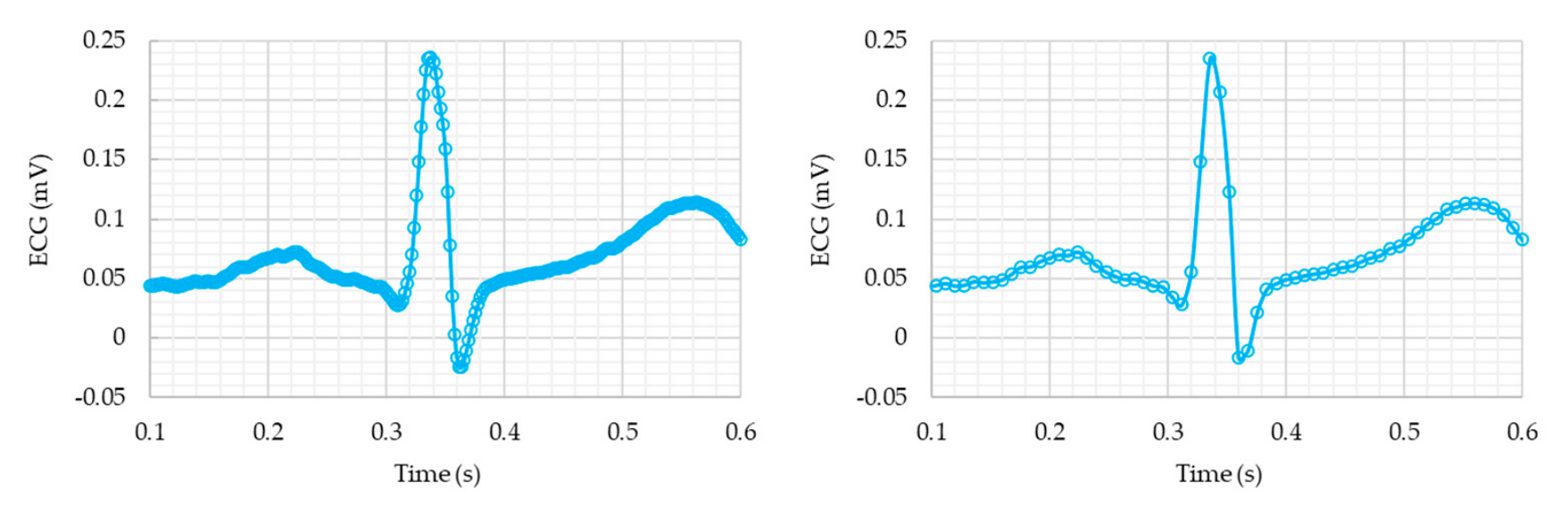
Figure 2.
Overview of the proposed ECG R-peak detection framework.
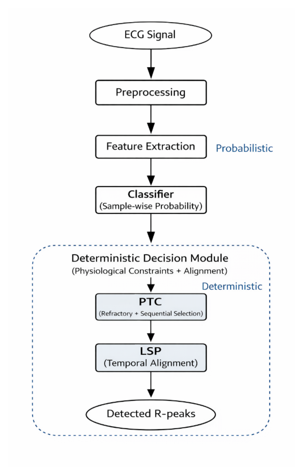
Figure 3.
Annotation for MIT-NSRDB (ID: 16265).
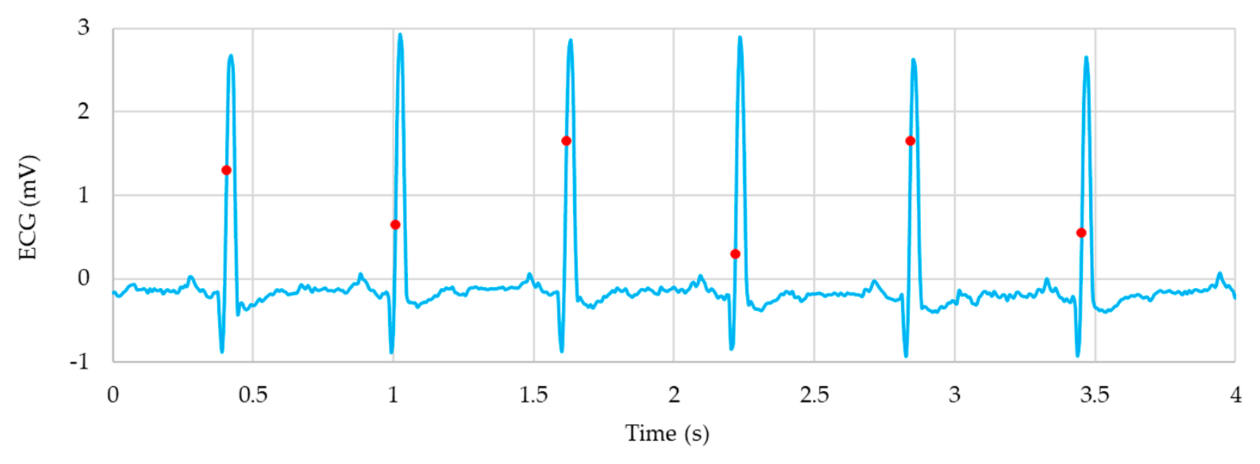
Figure 4.
Example of Silver-standard R-peak annotations in the PTB dataset. The blue line represents the ECG signal, and red vertical lines indicate the detected R-peak locations. Upper panel: patient104/s0306lre; lower panel: patient105/s0303lre. Only the first 10 seconds are shown for visualization.
Figure 4.
Example of Silver-standard R-peak annotations in the PTB dataset. The blue line represents the ECG signal, and red vertical lines indicate the detected R-peak locations. Upper panel: patient104/s0306lre; lower panel: patient105/s0303lre. Only the first 10 seconds are shown for visualization.
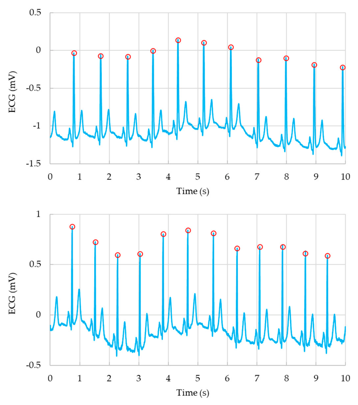
Figure 5.
Example of R-peak detection results with and without LSP in MIT-AD (360Hz, ID:100). Upper panel: detection with-out LSP. Lower panel: detection with LSP.
Figure 5.
Example of R-peak detection results with and without LSP in MIT-AD (360Hz, ID:100). Upper panel: detection with-out LSP. Lower panel: detection with LSP.
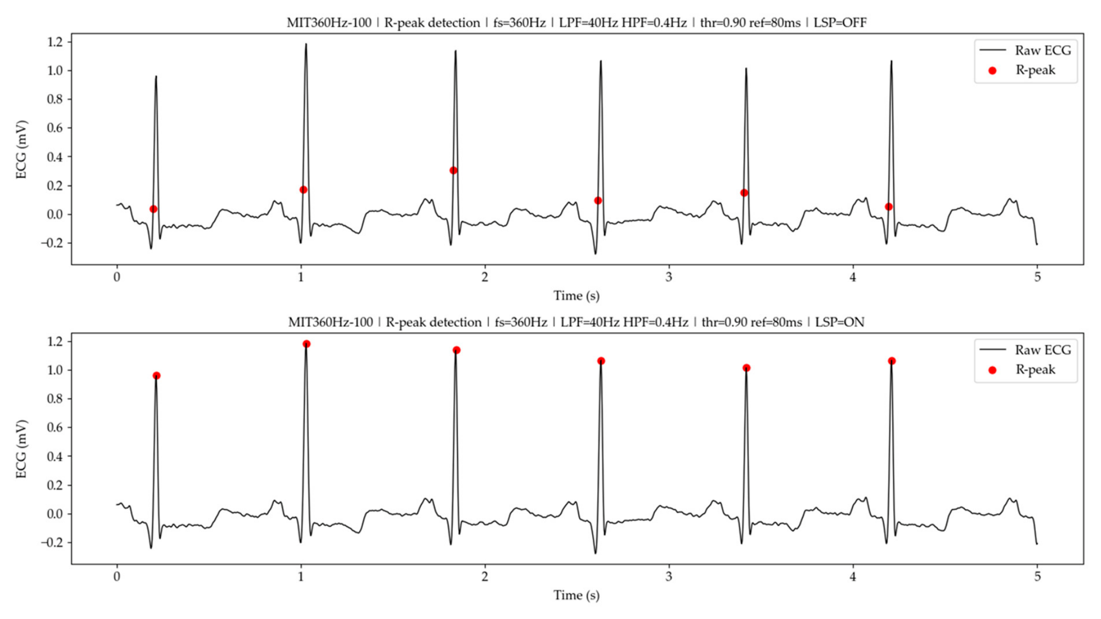
Figure 6.
Example of R-peak detection results with and without LSP in LUDB sinus rhythm (500Hz, ID:R3). Upper panel: detection with-out LSP. Lower panel: detection with LSP.
Figure 6.
Example of R-peak detection results with and without LSP in LUDB sinus rhythm (500Hz, ID:R3). Upper panel: detection with-out LSP. Lower panel: detection with LSP.
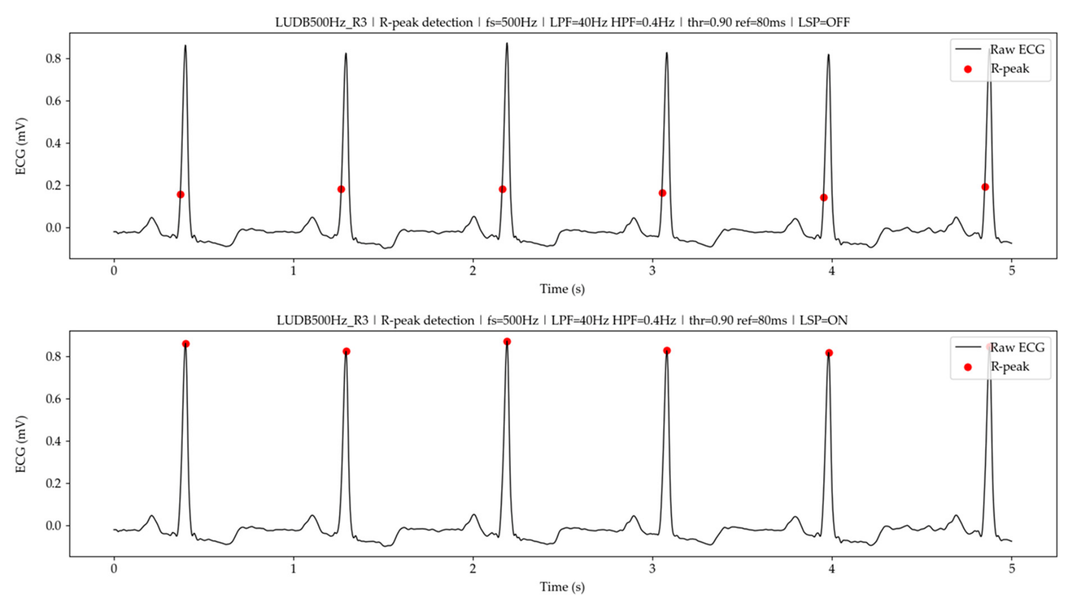
Figure 7.
Example of R-peak detection results with and without LSP in LUDB arrhythmia (500Hz, ID:R101_AF). Upper panel: detection with-out LSP. Lower panel: detection with LSP.
Figure 7.
Example of R-peak detection results with and without LSP in LUDB arrhythmia (500Hz, ID:R101_AF). Upper panel: detection with-out LSP. Lower panel: detection with LSP.
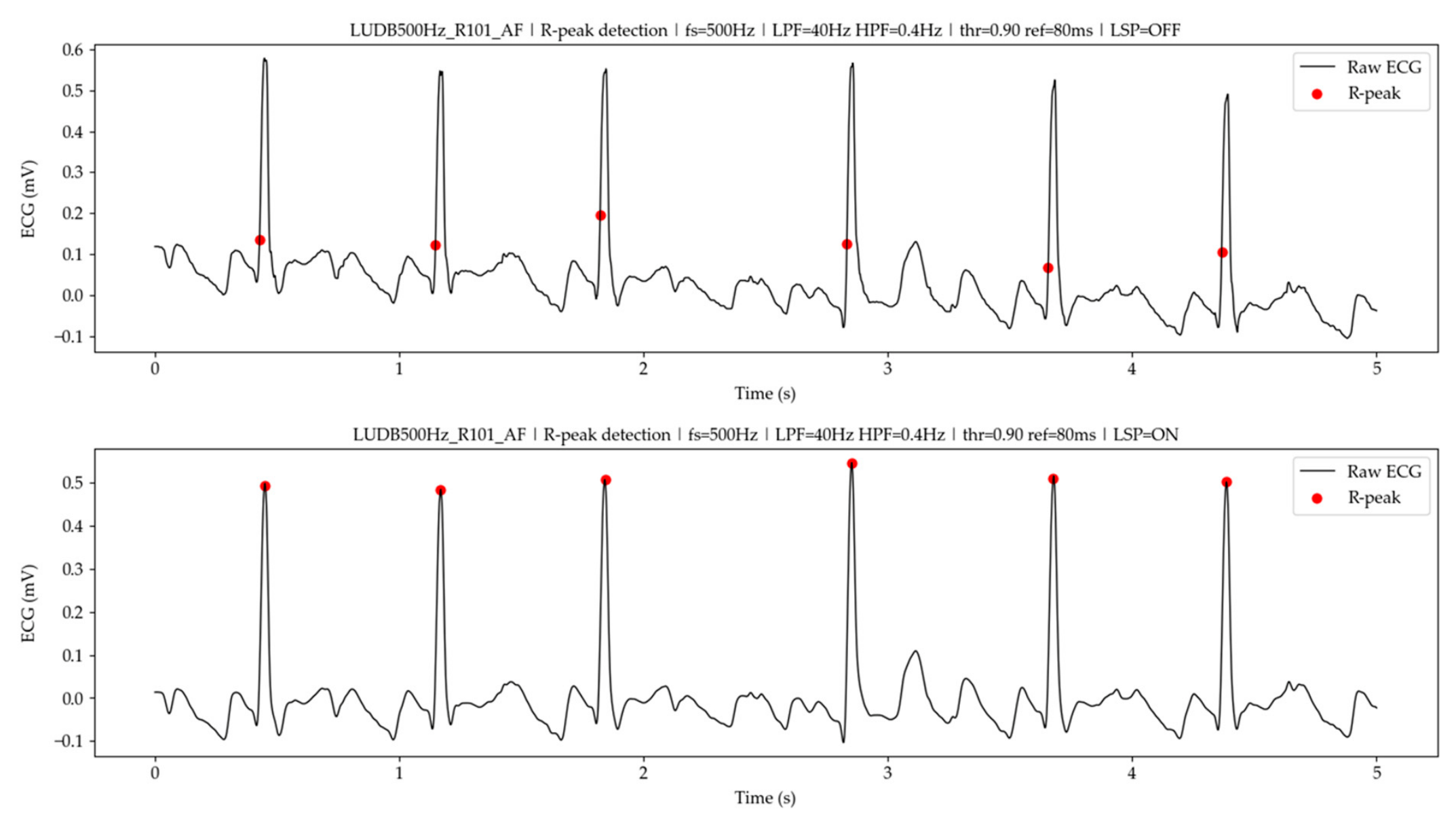
Figure 8.
Example of R-peak detection results with and without LSP in PTB healthy control (1000Hz, ID: patient104_s0306lre_l). Upper panel: detection with-out LSP. Lower panel: detection with LSP.
Figure 8.
Example of R-peak detection results with and without LSP in PTB healthy control (1000Hz, ID: patient104_s0306lre_l). Upper panel: detection with-out LSP. Lower panel: detection with LSP.
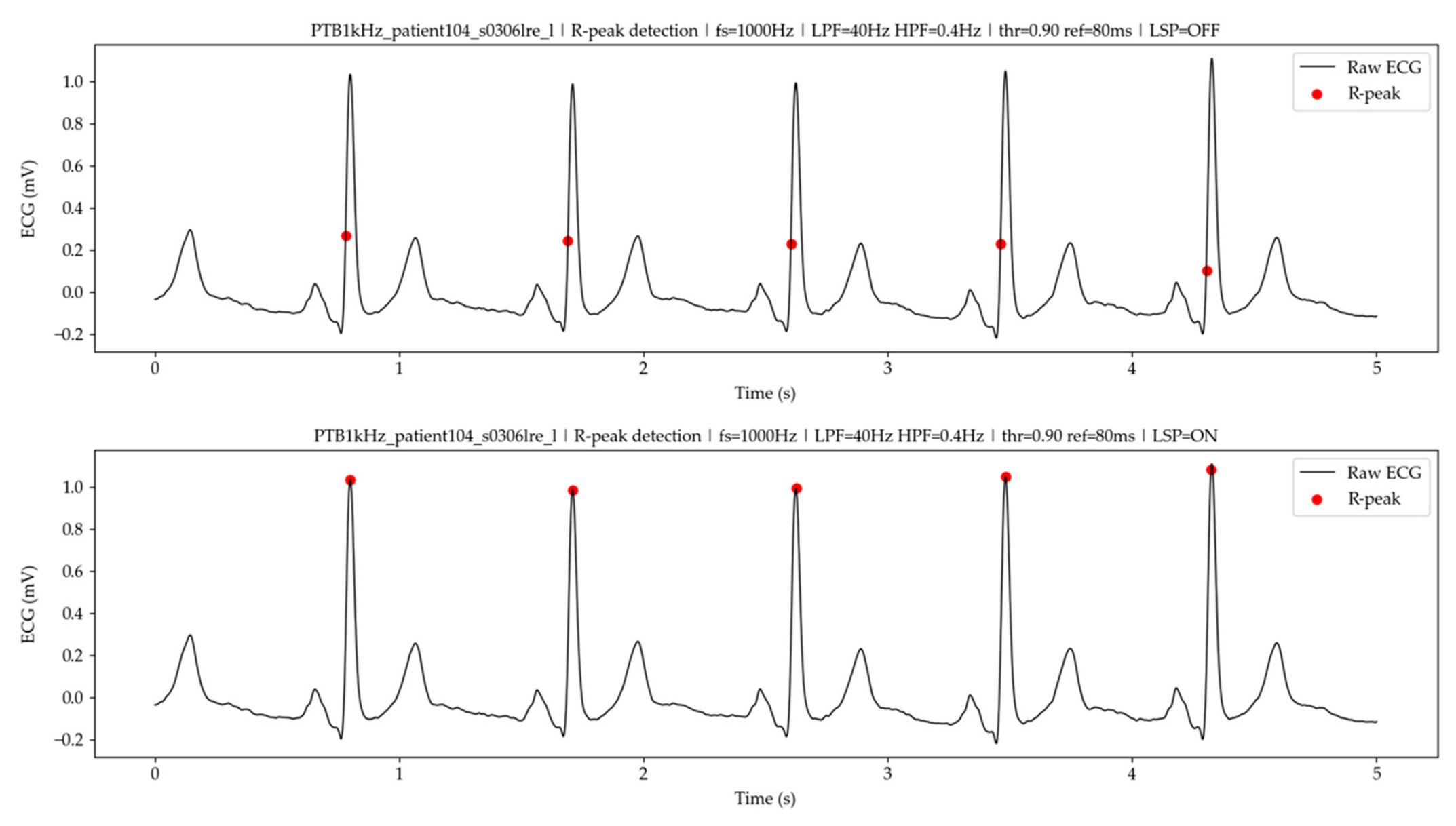

Table 1.
Definition of local morphological features (previous framework).
| Category | Formula | Name |
| Amplitude/statistical | mean | |
| std | ||
| left-right diff center - mean |
||
| Differential/curvature | d1 | |
| d2 | ||
| Slope/energy | slope | |
|
d1-energy |
||
| Amplitude | center value | |
| maximum | ||
| minimum |
Table 2.
Record-level split of the NSRDB dataset. Numbers indicate record IDs.
| Training set (14 records) |
16265 | 19090 | 16539 | 18177 | 16483 | 19093 | 16272 |
| 19088 | 16795 | 16786 | 16420 | 19140 | 19830 | 18184 | |
| Validation set (4 records) |
16273 | 16773 | 17453 | 17052 |
Table 3.
Sample-wise R-peak detection performance (mean ± SD) across six folds for different temporal window lengths. Metrics were computed using a matching tolerance of ±20 ms.
Table 3.
Sample-wise R-peak detection performance (mean ± SD) across six folds for different temporal window lengths. Metrics were computed using a matching tolerance of ±20 ms.
| win_len (ms) | Se | PPV | F1 |
| 16 | 0.941 ± 0.066 | 0.951 ± 0.056 | 0.946 ± 0.059 |
| 32 | 0.925 ± 0.082 | 0.946 ± 0.068 | 0.935 ± 0.073 |
| 48 | 0.938 ± 0.067 | 0.958 ± 0.051 | 0.948 ± 0.057 |
Table 4.
Sample-wise R-peak detection performance on the validation set using a fixed train–validation split at MIT-NSRDB (tolerance = ±20 ms). The upper panel reports detection metrics and optimized parameters, and the lower panel summarizes event counts. N denotes the total number of ECG samples (4 subjects).
Table 4.
Sample-wise R-peak detection performance on the validation set using a fixed train–validation split at MIT-NSRDB (tolerance = ±20 ms). The upper panel reports detection metrics and optimized parameters, and the lower panel summarizes event counts. N denotes the total number of ECG samples (4 subjects).
| win_len (ms) | Se | PPV | F1 | θR | refR (ms) |
| 16 | 0.998 | 0.998 | 0.998 | 0.95 | 80 |
| 32 | 0.999 | 0.998 | 0.998 | 0.90 | 80 |
| 48 | 0.998 | 0.998 | 0.998 | 0.90 | 40 |
| win_len (ms) | N (samples) | TP | FP | FN | |
| 16 | 8,678,400 | 70482 | 138 | 154 | |
| 32 | 8,678,400 | 70532 | 115 | 104 | |
| 48 | 8,678,400 | 70517 | 149 | 119 |
Table 5.
Optimal parameter set of the implementation model determined based on the highest validation F1 at MIT-NSRDB.
Table 5.
Optimal parameter set of the implementation model determined based on the highest validation F1 at MIT-NSRDB.
| Category | Parameter | Value |
| Pre-processing filters | LPF cutoff (Hz) | 40 |
| HPF cutoff (Hz) | 0.1 | |
| PTC | θR | 0.9 |
| refR (ms) | 80 | |
| win_len (ms) | 32 | |
| XGB | Number of estimators | 300 |
| Maximum depth | 4 | |
| Learning rate | 0.1 |
Table 6.
Feature importance of the XGB classifier based on gain and weight.
| Rank | Feature | Gain (%) | Rank | Feature | Weight |
| 1 | maximum | 72.30 | 1 | d1 | 602 |
| 2 | std | 13.30 | 2 | d1-energy | 500 |
| 3 | d1-energy | 8.90 | 3 | minimum | 496 |
| 4 | left-right diff | 1.80 | 4 | slope | 438 |
| 5 | d1 | 1.80 | 5 | d2 | 397 |
| 6 | slope | 1.20 | 6 | maximum | 389 |
| 7 | center value | 0.80 | 7 | mean | 373 |
| 8 | mean | 0.70 | 8 | center - mean | 339 |
| 9 | center - mean | 0.50 | 9 | std | 312 |
| 10 | minimum | 0.40 | 10 | left-right diff | 302 |
| 11 | d2 | 0.30 | 11 | center value | 243 |
Table 7.
Sample-wise R-peak detection performance under cross-frequency evaluation with and without LSP. Se, PPV, and F1 are reported as mean ± SD across records. TP, FP, and FN are reported as median [Q1–Q3]. Matching tolerance was ±20 ms. N denotes the total number of ECG samples per record.
Table 7.
Sample-wise R-peak detection performance under cross-frequency evaluation with and without LSP. Se, PPV, and F1 are reported as mean ± SD across records. TP, FP, and FN are reported as median [Q1–Q3]. Matching tolerance was ±20 ms. N denotes the total number of ECG samples per record.
| (a) MIT-AD (360 Hz) | ||||||||||||||||||||||||
| Condition | N | Se | PPV | F1 | TP | FP | FN | |||||||||||||||||
| LSP off (Default) | 648,000 | 0.606±0.365 | 0.629±0.352 | 0.615±0.358 | 1550 [530ー2029] | 457 [130ー1285] | 548 [80ー1573] | |||||||||||||||||
| LSP off (LPF = 10 Hz) | 648,000 | 0.020±0.021 | 0.157±0.227 | 0.032±0.037 | 24 [12ー73] | 418 [202ー1220] | 2150 [1849ー2542] | |||||||||||||||||
| LSP off (HPF = 0.4 Hz) | 648,000 | 0.610±0.367 | 0.626±0.355 | 0.616±0.360 | 1551 [535ー2031] | 457 [134ー1343] | 545 [44ー1559] | |||||||||||||||||
| LSP on (Default) | 648,000 | 0.860±0.226 | 0.904±0.190 | 0.878±0.208 | 2040 [1705ー2356] | 43 [18ー160] | 68 [5ー341] | |||||||||||||||||
| LSP on (LPF = 10 Hz) | 648,000 | 0.336±0.355 | 0.744±0.337 | 0.405±0.363 | 405 [97ー1233] | 17 [6ー64] | 1789 [545ー2285] | |||||||||||||||||
| LSP on (HPF = 0.4 Hz) | 648,000 | 0.871±0.222 | 0.904±0.192 | 0.885±0.206 | 2040 [1772ー2396] | 38 [10ー158] | 49 [1ー306] | |||||||||||||||||
| (b) LUDB (sinus rhythm, 500Hz) | ||||||||||||||||||||||||
| Condition | N | Se | PPV | F1 | TP | FP | FN | |||||||||||||||||
| LSP off (Default) | 5,000 | 0.845±0.296 | 0.692±0.224 | 0.755±0.255 | 8 [7ー9] | 2 [2ー4] | 0 [0ー1] | |||||||||||||||||
| LSP off (LPF = 10 Hz) | 5,000 | 0.118±0.197 | 0.279±0.325 | 0.136±0.202 | 0 [0ー2] | 2 [0ー7] | 8 [7ー9] | |||||||||||||||||
| LSP off (HPF = 0.4 Hz) | 5,000 | 0.88±0.266 | 0.708±0.207 | 0.782±0.232 | 8 [7ー9] | 2 [2ー3] | 0 [0ー1] | |||||||||||||||||
| LSP on (Default) | 5,000 | 0.917 ± 0.219 | 0.754 ± 0.147 | 0.820 ± 0.181 | 8 [8ー9] | 2 [2ー3] | 0 [0ー0] | |||||||||||||||||
| LSP on (LPF = 10 Hz) | 5,000 | 0.382±0.390 | 0.660±0.322 | 0.400±0.361 | 2 [0ー7] | 1 [0ー2] | 7 [2ー8] | |||||||||||||||||
| LSP on (HPF = 0.4 Hz) | 5,000 | 0.950 ± 0.167 | 0.772 ± 0.115 | 0.848 ± 0.136 | 9 [8ー10] | 2 [2ー3] | 0 [0ー0] | |||||||||||||||||
| (c) LUDB (arrhythmia, 500Hz) | ||||||||||||||||||||||||
| Condition | N | Se | PPV | F1 | TP | FP | FN | |||||||||||||||||
| LSP off (Default) | 5,000 | 0.799±0.325 | 0.640±0.246 | 0.705±0.277 | 7 [6ー10] | 3 [2ー4] | 0 [0ー3] | |||||||||||||||||
| LSP off (LPF = 10 Hz) | 5,000 | 0.072±0.151 | 0.202±0.307 | 0.082±0.161 | 0 [0ー1] | 2 [0ー4] | 8 [6ー11] | |||||||||||||||||
| LSP off (HPF = 0.4 Hz) | 5,000 | 0.826±0.309 | 0.660±0.236 | 0.730±0.268 | 7 [6ー11] | 3 [2ー4] | 0 [0ー2] | |||||||||||||||||
| LSP on (Default) | 5,000 | 0.909±0.215 | 0.738±0.162 | 0.808±0.178 | 8 [7ー11] | 2 [2ー3] | 0 [0ー0] | |||||||||||||||||
| LSP on (LPF = 10 Hz) | 5,000 | 0.322±0.388 | 0.614±0.328 | 0.330±0.353 | 1 [0ー5] | 1 [0ー2] | 7 [3ー10] | |||||||||||||||||
| LSP on (HPF = 0.4 Hz) | 5,000 | 0.946±0.170 | 0.758±0.116 | 0.837±0.138 | 8 [7ー11] | 2 [2ー3] | 0 [0ー0] | |||||||||||||||||
| (d) PTB (control, 1000Hz) | ||||||||||||||||||||||||
| Condition | N | Se | PPV | F1 | TP | FP | FN | |||||||||||||||||
| LSP off (Default) | 120,012 | 0.896±0.211 | 0.864±0.201 | 0.876±0.204 | 120 [110ー136] | 8 [2ー18] | 2 [0ー9] | |||||||||||||||||
| LSP off (LPF = 10 Hz) | 120,012 | 0.169±0.208 | 0.343±0.323 | 0.207±0.233 | 9 [1ー36] | 27 [10ー50] | 113 [90ー131] | |||||||||||||||||
| LSP off (HPF = 0.4 Hz) | 120,012 | 0.910±0.232 | 0.890±0.230 | 0.899±0.230 | 123 [112ー142] | 3 [1ー12] | 0 [0ー3] | |||||||||||||||||
| LSP on (Default) | 120,012 | 0.954±0.137 | 0.922±0.127 | 0.935±0.129 | 125 [114ー143] | 4 [1ー13] | 0 [0ー1] | |||||||||||||||||
| LSP on (LPF = 10 Hz) | 120,012 | 0.320±0.325 | 0.595±0.375 | 0.379±0.340 | 19 [3ー80] | 11 [3ー23] | 101 [46ー125] | |||||||||||||||||
| LSP on (HPF = 0.4 Hz) | 120,012 | 0.963±0.142 | 0.944±0.145 | 0.953±0.143 | 126 [115ー145] | 1 [0ー4] | 0 [0ー0] | |||||||||||||||||
Table 8.
Temporal localization error (mean ± SD) with and without LSP. Errors are defined as the difference between detected and reference R-peak timings (detected − reference, in ms). N denotes the number of true-positive matched detections within a ±20 ms tolerance window.
Table 8.
Temporal localization error (mean ± SD) with and without LSP. Errors are defined as the difference between detected and reference R-peak timings (detected − reference, in ms). N denotes the number of true-positive matched detections within a ±20 ms tolerance window.
| Dataset | Corrected LSP | Number of TP | Mean ± SD (ms) |
|---|---|---|---|
| MIT-AD (360 Hz) | Without | 64,068 | –14.5±7.0 |
| With | 91,050 | –1.3±4.4 | |
| LUDB (Sinus,500 Hz) | Without | 1,084 | –13.1±6.1 |
| With | 1,178 | 1.4±2.5 | |
| LUDB (Arrhythmia,500 Hz) | Without | 431 | –13.0±7.0 |
| With | 491 | 1.4±3.4 | |
| PTB (control, 1000 Hz) | Without | 9,006 | –13.9±7.3 |
| With | 9,580 | –0.6±3.0 |
Disclaimer/Publisher’s Note: The statements, opinions and data contained in all publications are solely those of the individual author(s) and contributor(s) and not of MDPI and/or the editor(s). MDPI and/or the editor(s) disclaim responsibility for any injury to people or property resulting from any ideas, methods, instructions or products referred to in the content. |
© 2026 by the authors. Licensee MDPI, Basel, Switzerland. This article is an open access article distributed under the terms and conditions of the Creative Commons Attribution (CC BY) license.
Copyright: This open access article is published under a Creative Commons CC BY 4.0 license, which permit the free download, distribution, and reuse, provided that the author and preprint are cited in any reuse.