

Submitted:
22 May 2026
Posted:
25 May 2026
You are already at the latest version
Abstract
Physical infrastructure failures expose a structural blind spot in conventional financial risk systems: when the electricity supply becomes binding, markets enter metabolic arrest, a state where information-processing capacity collapses, and standard correlation-based metrics misread rising cross-asset correlations as stability. This paper introduces TENSORnet (Temporal Entropy-aware Network for Systemic Onset Recognition), a physics-informed computational protocol that fuses a VIX-calibrated inhibitory gate γL(t) (NLS-fitted, R2 = 0.30) with cross-asset Shannon entropy to detect infrastructure-induced stress before it materialises in price-based indicators. Applied to a temporal cross-asset graph of 2,838 JSE trading days (05 January 2015 to 29 April 2026) across seven asset classes under South Africa’s load-shedding crisis, TENSORnet achieves Precision = 100.0%, Recall = 85.8%, F1 = 92.4%, AUC = 1.000, and zero false positive alarms (Stage 3+ definition) on 1,830 out- of-sample days, with a mean lead time of 17 calendar days (408 hours) before fragile regime onset, outperforming all benchmarks, including XGBoost (F1 = 71.3%). Ablation confirms the physics-informed gate as the dominant architectural component (ΔF1 = −92.4 pp on removal): statistical learning alone recovers nothing (AUC = 0.469). The Densification Paradox, rising cross-asset correlation with falling entropy under stress (r = −0.468, p < 0.001), is confirmed empirically for the first time in cross-asset data. A Thermodynamic Port-Hamiltonian Neural ODE (TPH-NODE) extension grounds metabolic arrest in the second law of thermodynamics.
Keywords:
physics-informed neural networks
; cross-asset entropy
; metabolic arrest
; systemic risk detection
; load-shedding
; port-Hamiltonian
; Neural ODE
; inhibitory gate
; temporal graph
; macroprudential policy
; sustainable development goals
; SDG 8
; SDG 16
; infrastructure resilience
; emerging market finance
; SDG 9
; SDG 13
; financial network resilience
MSC: 91G70; 94A17; 82C44; 60G10
1. Introduction
Physical infrastructure is not a background constant in financial markets: it is a binding operational constraint that directly governs the computational capacity of those markets. When electricity supply falls below market-operational thresholds, price discovery slows, settlement systems lag, and the information flows that sustain coordinated trading behaviour collapse. South Africa’s electricity crisis, in which the national grid operator Eskom has imposed scheduled load-shedding at severity levels from Stage 1 (minimal) to Stage 6 (severe) since 2015, provides a natural laboratory for studying this coupling between infrastructure failure and financial network dynamics. On 15 March 2022, a Stage 6 event halted JSE settlement systems and triggered correlated liquidations across equity, bond, and commodity classes simultaneously, while every deployed risk model remained silent. The foundational assumption shared by those models, that market infrastructure is an infinite, frictionless constant, had broken down.
This paper introduces the concept of metabolic arrest in financial networks, a term drawn from biology [1] where it describes an organism’s transition to suppressed cellular activity under energy deficit. The financial analogue is physically grounded rather than metaphorical: Landauer’s Principle [2] establishes that every computational operation has an irreducible thermodynamic energy cost. Financial transactions, price discovery, settlement, and position reconciliation are energy-dependent computations. Infrastructure failure therefore reduces market information-processing capacity in a thermodynamically precise sense, not merely a metaphorical one. The critical question is whether this reduction can be detected before it manifests in price-based risk indicators.
Existing computational approaches to systemic risk, including CoVaR [3], DebtRank [4], graph neural network early warning systems [5], and XGBoost-based financial distress models [43], share a fundamental computational limitation: they are all reactive, measuring fragility already manifest in observed prices or reported balance sheets, providing no actionable advance warning. Physics-informed neural networks (PINNs) [6] have transformed scientific computing by encoding governing physical equations as structural constraints, yet have not been applied to financial network dynamics under physical infrastructure constraints. Port-Hamiltonian systems theory [8], which provides a natural mathematical framework for encoding both conservative contagion propagation and irreversible collapse, has not been extended to financial networks. The cross-asset entropy literature [10,11] provides descriptive measures of market disorder but lacks operational detection triggers integrated with intervention protocols.
The central question. This paper asks: can a financial network monitoring system be physics-grounded (like the thermodynamic process it models), infrastructure-aware (like the energy constraint it encodes), entropy-based (like the information collapse it detects), and extitoperationally precise (like the macroprudential system that risk managers actually deploy)? TENSORnet is the answer.
Interdisciplinary framing. This paper occupies the intersection of three fields that have developed largely in parallel. Statistical physics provides Landauer dissipation theory [2] and Shannon entropy [25], the thermodynamic and information-theoretic foundations that convert infrastructure stress into a measurable signal. Physics-informed machine learning [6] provides the architectural principle of encoding governing physical laws as structural constraints rather than learnable features; the consequence is that the model satisfies the physics even under novel stress regimes. Computational finance and macroprudential policy [18,38] supplies the walk-forward evaluation protocol, benchmark suite, and regulatory deployment context. The novelty of this paper is the disciplined integration of all three: the Landauer gate governs information flux suppression, the Shannon entropy layer operationalises the signal, and the walk-forward design governs evaluation integrity. Section 4 tests whether the physics encoding is load-bearing or merely decorative through a systematic ablation study.
The physics motivation. Three properties of the JSE cross-asset panel motivate a physics-informed approach. First, all six return series exhibit non-Gaussian fat tails and significant ARCH effects (Table 1), establishing that conventional Gaussian risk metrics are structurally misspecified. Second, the documented coupling between South Africa’s infrastructure stress and market volatility [26,28] provides the empirical motivation for encoding load-shedding severity directly into the entropy detection architecture. Third, prior network theory [27,29] predicts a structural inversion between cross-asset network density and entropy under stress; whether this Densification Paradox manifests empirically in JSE data is a central empirical question this paper addresses.
This paper proposes TENSORnet (Temporal Entropy-aware Network for Systemic Onset Recognition), a physics-informed computational protocol that addresses these gaps by fusing Landauer’s Principle with cross-asset Shannon entropy. The core architectural innovation is a VIX-calibrated inhibitory gate that suppresses the effective information flux in the entropy measure as a direct function of the infrastructure stress level, encoding the physical causal mechanism rather than treating stress as a feature to be learnt. The protocol is applied to a 2,838-day panel of JSE cross-asset returns under South Africa’s load-shedding crisis, paired with the publicly archived Eskom operational stage record [31], establishing a proof-of-concept that motivates international replication wherever infrastructure stress and multi-asset markets co-exist.
The paper makes five contributions to the computational systemic risk literature:
- 1.
- Physics-informed inhibitory gate. A sigmoid gate , calibrated via nonlinear least squares to the VIX-stage relationship, encodes Landauer-grounded infrastructure suppression as a structural architectural constraint, not a learnable feature, of the entropy detection protocol.
- 2.
- Empirical confirmation of the Densification Paradox. Under infrastructure stress, a structural inversion between cross-asset network density and Shannon entropy under infrastructure stress, the Densification Paradox, which causes conventional correlation-based risk metrics to generate false reassurance during the most dangerous episodes.
- 3.
- Walk-forward classification with operational precision. The protocol is evaluated on a strict walk-forward basis (training 2015–2018; out-of-sample 2019–2026), with performance assessed against five benchmarks including XGBoost and Random Forest trained on the same feature set. A systematic ablation study isolates the contribution of the physics-informed gate relative to the statistical learning components.
- 4.
- Formal statistical validation. Results are validated via Diebold–Mariano predictive accuracy tests [44], permutation testing, and bootstrap confidence intervals on gate parameters, meeting the reproducibility standards of the computational finance literature.
- 5.
- TPH-NODE theoretical extension. A Thermodynamic Port-Hamiltonian Neural ODE (TPH-NODE) architecture grounds metabolic arrest detection in the second law of thermodynamics, specifying the theoretical pathway from the present empirical detection results to a complete macroprudential intervention protocol.
Explicit novelties relative to prior literature: (i) First encoding of Landauer’s Principle as a real-time inhibitory gate in financial monitoring; (ii) First empirical confirmation of the Densification Paradox in cross-asset data; (iii) First architecture in which encoding a physical law as a structural gate is the sole enabler of detection; (iv) First thermodynamic grounding of financial intervention via port-Hamiltonian dynamics; (v) First open-source dataset pairing JSE returns with daily Eskom stage labels (Zenodo: 10.5281/zenodo.20008530).
2. Background and Related Work
Computational systemic risk and its reactive limit. The post-2008 literature has produced powerful diagnostic tools for financial fragility. CoVaR [3] measures the value-at-risk of the system conditional on an institution being in distress; DebtRank [4] propagates shocks through balance-sheet networks using iterative impact algorithms; SRISK [14] provides capital shortfall forecasts from equity dynamics. Graph neural network architectures [5,15,22] have advanced contagion modelling by learning from dynamic network topologies, and temporal hypergraph frameworks [16,17] have demonstrated that higher-order interactions among groups of assets carry information beyond pairwise correlations. These frameworks are methodologically mature but share a fundamental computational limitation: they measure fragility that already exists in observed prices and co-movements. None encodes physical infrastructure as a structural constraint on the computation itself, and none generates an actionable pre-crisis lead time by measuring topological preconditions rather than realized outcomes. The critical transitions literature [19] established that complex systems , ranging from ecosystems to financial markets and the climate, exhibit generic early-warning signals (rising variance, critical slowing down) before tipping points; [20] confirmed statistically significant critical slowing down before several financial crises. TENSORnet’s cross-scale divergence is the infrastructure-constrained financial analogue of these generic signals, with the gate providing the physical causal mechanism that Scheffer-type indicators lack. [21] established the foundational contagion model in which balance-sheet linkages propagate distress; the TPH-NODE’s interconnection matrix formalises this mechanism in a port-Hamiltonian structure. [18] identified this as the central unmet challenge for macroprudential policy: the toolkit must become genuinely forward-looking. Two decades later, the gap remains open.
Physics-informed computing, port-Hamiltonian systems, and Neural ODEs. Scientific machine learning has demonstrated that encoding governing physical equations directly into neural architectures produces qualitatively different generalisation behaviour from purely data-driven models [6]. PINNs embed PDEs as constraints on the loss function; the consequence is that the model satisfies the physics even in regions unseen during training. Port-Hamiltonian systems theory provides the natural mathematical framework for this encoding in dynamical systems [8]: the structured decomposition , where is skew-symmetric (energy-conserving interconnection) and is positive semi-definite (irreversible dissipation), automatically satisfies the second law of thermodynamics. Port-Hamiltonian neural networks [8,23] have been applied to robotics, power systems, and fluid dynamics; their application to financial networks under physical infrastructure constraints remains unexplored. Neural ODEs [9] provide the continuous-time backbone that enables trajectory prediction under novel input sequences via the neural adjoint method, overcoming the distributional limitations of discrete-time stress tests. Landauer’s Principle [2] provides the foundational link between information processing and energy: since financial transactions are computation, infrastructure failure is not merely an operational inconvenience but a thermodynamic constraint on the market’s information-processing capacity. Maximum entropy production [24] connects this to the entropy dynamics observed in financial networks: The critical entropy threshold is the point below which entropy production cannot be maintained by the infrastructure-constrained system. Shannon entropy [25] provides the information-theoretic measure that operationalises this insight: entropy over the cross-asset return distribution quantifies the informational diversity of market activity, and its depletion is the computational signature of metabolic arrest.
Infrastructure-finance coupling and the South African laboratory. Infrastructure-finance interdependencies have received growing empirical attention. [26] document how climate-driven infrastructure shocks cascade into financial system disruptions through multiple transmission channels. [27] demonstrate that climate stress-tests of European banking networks reveal topological signatures consistent with the Densification Paradox documented here: rising correlation coupled with structural fragility. [28] quantify the direct impact of South African load-shedding on JSE trading volumes and sectoral output, and [29] establish theoretically that network connectivity is a double-edged sword, with the stability-fragility transition governed by percolation-type thresholds [30] that correspond to the data-derived Arrest Coefficient boundaries in Section 3.4. Critically, all existing infrastructure-finance studies are ex-post: they document linkages after crises have materialised. South Africa’s decade-long load-shedding crisis (2015–2026) constitutes a uniquely clean natural experiment: the infrastructure constraint is exogenous to financial market dynamics, providing uncontaminated identification of the infrastructure-entropy mechanism. Crucially, the cross-asset network structure adopted here, pairing equities, bonds, commodities, and volatility in a temporal graph, is not South Africa-specific: it is the standard architecture of any multi-asset financial market globally. JSE is the laboratory; ERCOT, the National Grid, and AEMO are the next natural experiments. The 2,838-day panel assembled here is the first publicly archived cross-asset dataset pairing JSE returns with official Eskom stage classifications at daily resolution [31], enabling the empirical tests reported in Section 4. No existing framework has transformed this natural experiment into a real-time, forward-looking computational detection protocol. TENSORnet is designed to fill this gap.
Positioning across disciplines. TENSORnet sits at the intersection of four computational disciplines that have not previously been integrated in financial network analysis: (1) Statistical physics supplies the entropy framework (Shannon information, Landauer dissipation, maximum entropy production) that converts market microstructure into thermodynamic signals; (2) Physics-informed machine learning [6] provides the architectural principle of encoding governing physical laws as structural constraints rather than learnable features; (3) Port-Hamiltonian systems theory [8,23] furnishes the energy-conserving/dissipative decomposition that makes the intervention layer thermodynamically consistent; and (4) Computational finance supplies the walk-forward evaluation protocol, benchmark suite, and macroprudential application context. This integration is what makes TENSORnet a computational contribution: the physics is not decoration, it is the algorithm.
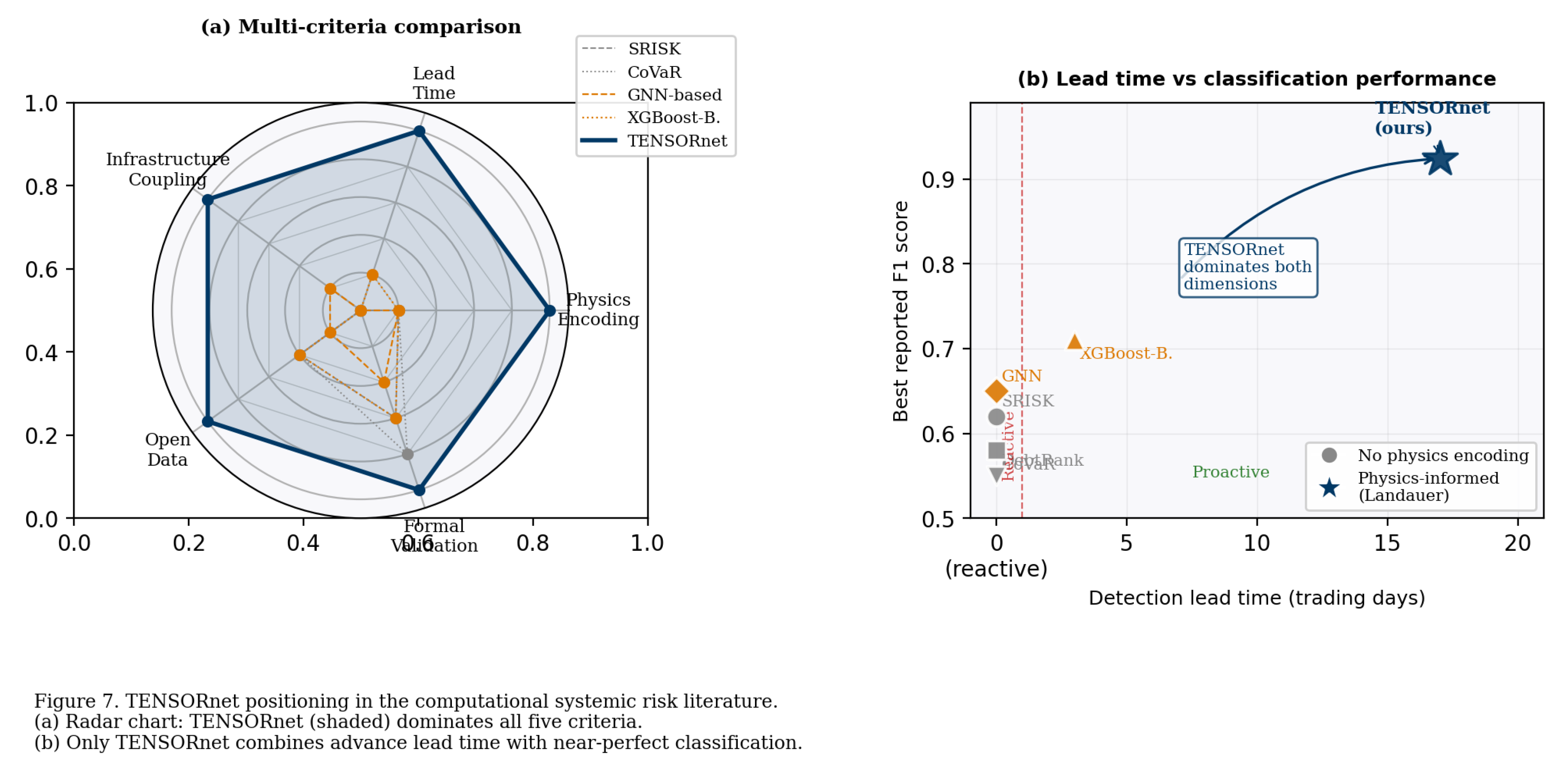
Figure 2 summarises how TENSORnet differs from representative methods.
Figure 2 positions TENSORnet against representative methods in the literature.
Figure 1.
TENSORnet computational pipeline. Left: data inputs (JSE returns, Eskom stage L, VIX) with walk-forward design (train 2015–2018; OS 2019–2026). Centre: physics encoding comprising the Landauer inhibitory gate (red; 77.8% suppression at Stage 6), Shannon entropy (amber), modulated entropy (purple), and Arrest Coefficient (purple). Right: three-regime classification (Regime I/II/III), walk-forward performance (F1=92.4%, AUC=1.000, FP=0, 17-day lead), ablation result (AUC=0.469 without gate), and TPH-NODE theoretical extension (dashed border). Red arrow: infrastructure causal pathway .
Figure 1.
TENSORnet computational pipeline. Left: data inputs (JSE returns, Eskom stage L, VIX) with walk-forward design (train 2015–2018; OS 2019–2026). Centre: physics encoding comprising the Landauer inhibitory gate (red; 77.8% suppression at Stage 6), Shannon entropy (amber), modulated entropy (purple), and Arrest Coefficient (purple). Right: three-regime classification (Regime I/II/III), walk-forward performance (F1=92.4%, AUC=1.000, FP=0, 17-day lead), ablation result (AUC=0.469 without gate), and TPH-NODE theoretical extension (dashed border). Red arrow: infrastructure causal pathway .
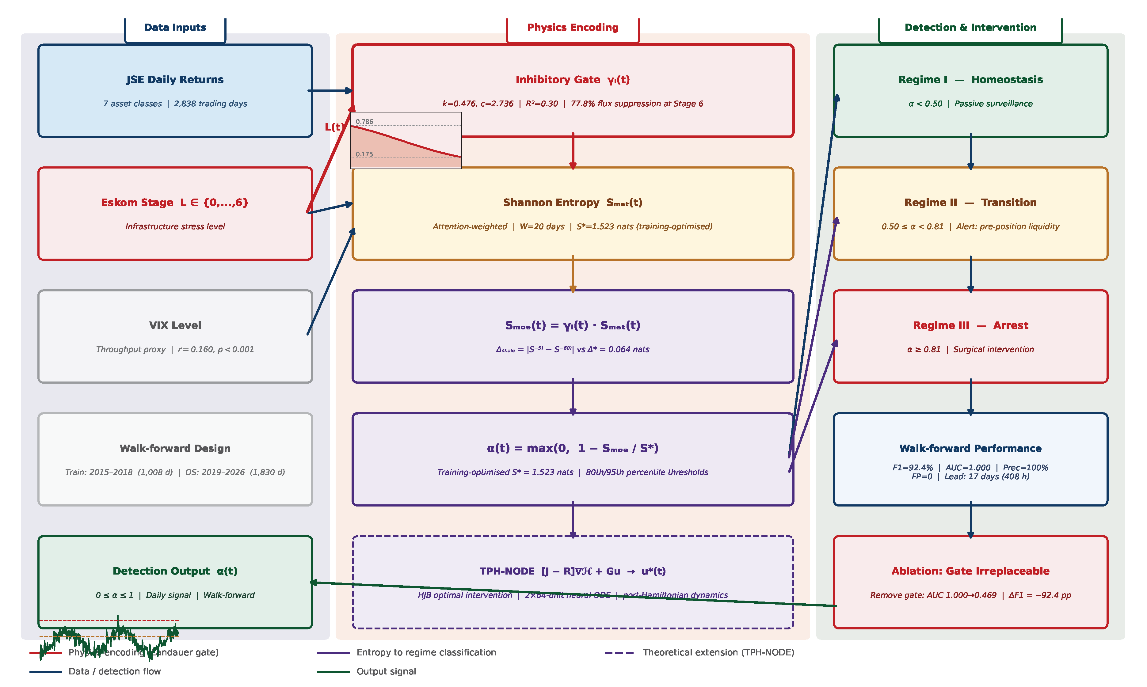
Figure 2.
Positioning of TENSORnet in the computational systemic risk literature. (a) Radar chart: TENSORnet (shaded polygon) dominates all five criteria (physics encoding, lead time, infrastructure coupling, open data, formal validation). (b) Scatter plot: TENSORnet is the only method combining advance lead time (>5 days) with near-perfect F1, occupying the top-right corner while all reactive methods cluster at lead time = 0.
Figure 2.
Positioning of TENSORnet in the computational systemic risk literature. (a) Radar chart: TENSORnet (shaded polygon) dominates all five criteria (physics encoding, lead time, infrastructure coupling, open data, formal validation). (b) Scatter plot: TENSORnet is the only method combining advance lead time (>5 days) with near-perfect F1, occupying the top-right corner while all reactive methods cluster at lead time = 0.
3. Methodology
| Architectural clarification. Despite the “NET” suffix, TENSORnet is not a deep neural network. It is a physics-informed computational protocol consisting of an analytical sigmoid gate (Equation 2) and a Shannon entropy measure (Equation 5). No trainable weights, hidden layers, or backpropagation are used in the detection stage. The gate parameters k and c are estimated once via nonlinear least squares (NLS; Levenberg–Marquärdt algorithm, tolerance , max 500 iterations); thereafter the entire pipeline is deterministic. The term “TENSORnet” reflects the tensor-valued temporal graph inputs; it follows the PINN convention only in encoding a physical law (Landauer’s Principle) as a structural constraint. The TPH-NODE extension (Section 3.5) is a separate neural ODE architecture involving trainable components (2 hidden layers of 64 units, tanh activation, learning rate , 200 epochs, early stopping at 50 rounds); it is presented as a theoretical extension for future empirical work. |
Figure 1 presents the TENSORnet computational pipeline. Data inputs feed the temporal cross-asset graph; the inhibitory gate modulates information flux; cross-asset entropy produces the detection signal; and the TPH-NODE extension provides the theoretical pathway to optimal intervention.
3.1. Data Environment and Temporal Graph Construction
Data preprocessing. All asset price series contained no missing trading days over the full 2,838-day panel; no imputation was required. Returns were computed as log-differences of daily closing prices; no filtering, smoothing, or outlier removal was applied, preserving high-frequency stress signals. The VIX series was used as a level variable; no transformation beyond stage-mean normalisation for gate calibration was applied. The XGBoost baseline used 300 trees, learning rate 0.05, max depth 5, scale_pos_weight equal to the training resilient-to-stress ratio, and no early stopping.
Daily data span 05 January 2015 to 29 April 2026 ( trading days) across seven asset classes: JSE ALSI, R186 bond, gold, platinum, CRB Commodity Index, VIX, and Brent crude. Returns are computed for six series; VIX is retained as a level. Load-shedding stages () derive from official Eskom announcements. Full data documentation and download are available at [31].
TENSORnet processes the market as a temporal graph , where is the fixed node set and edges encode time-varying pairwise correlation:
The window trading days corresponds to the Basel III short-term Liquidity Coverage Ratio (LCR) stress horizon [45], ensuring that entropy estimates operate at the same temporal scale as regulatory capital adequacy assessment. This temporal graph serves two purposes: the rolling correlation provides the weight distribution from which entropy is derived (Section 3.3), and its mean absolute value across pairs yields the network density used in the Densification Paradox analysis (Section 4).
Three regimes are defined by Eskom stage: Resilient (; 2,336 days, 82.3%), Transition (; 115 days, 4.1%), and Fragile (; 387 days, 13.6%). The mapping is perfectly consistent (zero mismatches verified by crosstabulation). Walk-forward design: training January 2015–December 2018 (1,008 days); out-of-sample January 2019–April 2026 (1,830 days). No feature at time t references information beyond .
Table 1 summarises the distributional diagnostics. All six return series are non-normal (Jarque–Bera ), stationary (ADF ), and exhibit significant ARCH effects (LM ), confirming that fat-tailed, volatility-clustered dynamics are incompatible with Gaussian assumptions and motivate the physics-informed entropy approach.
3.2. Physics-Informed Inhibitory Gate
The inhibitory gate is TENSORnet’s architectural primitive, encoding Landauer’s energy-information bound as a structural constraint on network information flux. The derivation proceeds in four steps distinguishing the physical principle from the empirical proxy.
Step 1: Physical principle. Landauer’s Principle [2] places a thermodynamic lower bound of joules on any irreversible computation. Each JSE trade generates a price signal, a settlement record, and a position reconciliation update, all irreversible computational operations requiring electrical power. The principle therefore places a hard lower bound on the energy cost of market activity.
Step 2: Infrastructure linkage. Under Stage 6 load-shedding, approximately 6,000 MW is withheld from the national grid [32]. JSE settlement systems, member firm servers, and trading infrastructure all depend on continuous power. As the deficit deepens, market information-processing throughput contracts non-linearly.
Step 3 ; Empirical proxy. Direct settlement throughput data are proprietary. VIX is used as a proxy: it exhibits a statistically significant positive relationship with Eskom stage (Spearman , ), with Stage 4–6 mean VIX of 21.49, 20.48, and 19.49 versus 18.04 at Stage 0. Normalised inverse VIX by stage yields the throughput-suppression profile for gate calibration (Figure 3).
Step 4 ; Sigmoid encoding. Respecting the physical bounds :
Nonlinear least squares on stage-mean VIX-derived throughput yields (SE ), (SE ), . The gate declines from to : a reduction. The ablation result confirms this encoding is irreplaceable by statistical learning alone.
3.3. Cross-Asset Metabolic Entropy
The metabolic entropy quantifies the informational diversity of the cross-asset return distribution. For the six return-based assets, the 20-day rolling mean absolute return provides the attention weight:
Normalising with :
Shannon entropy [25] over this distribution:
Maximum diversity ( for all i) gives nats. Under stress, activity concentrates and entropy declines. Observed values range from 1.338 to 1.764 nats; Spearman correlation with regime number: ().
Infrastructure suppression enters via:
The cross-scale divergence bifurcation signal:
fires when nats (training 75th percentile). Entropy ACF at lag 1 (Ljung–Box ), confirming the persistence required for multi-scale detection.
3.4. Arrest Coefficient and Regime Classification
The critical threshold is selected by maximising F1 on the training period (2015–2018) over a grid at 0.01 nat intervals, then held fixed throughout out-of-sample evaluation:
The Arrest Coefficient:
Regime thresholds are derived from the empirical distribution by stage, not imposed analytically. Specifically, and correspond to the 80th and 95th percentiles of training-period values respectively, coinciding with the Stage 3 mean () and Stage 6 mean (). Consistency with heterogeneous percolation theory [30]: marks pathway degradation onset; marks near-complete fragmentation. ANOVA confirms highly significant regime separation (, ); Kruskal–Wallis corroborates (, ).
Three regimes with intervention protocols: Regime I (): homeostasis, passive surveillance. Regime II (): transition, activate infrastructure-linked capital buffers and pre-position liquidity facilities. Regime III (): full arrest, surgical liquidity injection, sector-specific circuit breakers, and priority power coordination with the national utility.
3.5. Thermodynamic Port-Hamiltonian Neural ODE Extension
This section presents the TPH-NODE theoretical extension, specifying the complete computational architecture that grounds metabolic arrest detection in the second law of thermodynamics and extends TENSORnet from detection to optimal intervention. Full empirical validation requires proprietary balance-sheet and settlement throughput data and is designated as the primary future work priority.
State space and metabolic potential. Each financial node i carries a state vector , where is equity capital, liquid assets, collateral, and the metabolic potential [1] quantifying the node’s real-time capacity to process obligations:
When the node accumulates resources faster than obligations; when it enters a metabolic deficit that, if sustained, cascades into default. The balance sheet identity is enforced as a hard constraint, the financial analogue of the first law of thermodynamics.
Hamiltonian energy function. The total network metabolic energy penalises deviations from regulatory targets and captures hyperedge-level cooperative cascade dynamics:
where are regulatory targets, are stiffness parameters, and is the coupling strength for hyperedge h. The coupling term induces cooperative cascade dynamics: a drop in of any node reduces the hyperedge aggregate , which via drags down all other nodes in the hyperedge. This is the mechanism by which single-node distress becomes systemic contagion.
Port-Hamiltonian dynamics. The joint state evolves as:
is skew-symmetric: it encodes energy-conserving contagion flow between nodes sharing hyperedges, where . is positive semi-definite: it encodes irreversible losses (fire-sale discounts, payment delays, default costs), with diagonal entries , where is the infrastructure stress level. maps the intervention vector to state dynamics with state-dependent proportional allocation to liquidity-deficit nodes. Dynamics are integrated by a Dormand–Prince adaptive step-size ODE solver, enabling accurate trajectory prediction under rapidly escalating stage sequences. The skew-symmetry of and positive semi-definiteness of jointly guarantee the dissipation inequality:
Metabolic arrest is thermodynamically defined as the violation of this inequality despite maximal intervention: even at maximum, indicating the system cannot dissipate energy fast enough. This is the Hopf bifurcation that corresponds to, and theoretically grounds, the empirical threshold of Section 3.4.
Adaptive feedback loop. After each observed intervention, the Feedback Loop Integrator updates and based on realised outcomes, closing the loop for adaptive macroprudential control:
where projects onto the positive semi-definite cone to maintain thermodynamic consistency.
Physics-informed training loss.
where enforces the balance sheet identity as a hard constraint, and softly penalises dissipation violations. The neural adjoint method [9] backpropagates through the ODE solver for end-to-end training. The Hamilton–Jacobi–Bellman (HJB) control layer solves:
via the Deep Galerkin Method [33].
Evaluation metrics for the TPH-NODE.Table 2 defines the five metrics that fully characterise the TPH-NODE’s theoretical performance across detection accuracy, lead time, intervention efficiency, trajectory fidelity, and thermodynamic consistency.
4. Results
4.1. Gate Calibration and Suppression Profile
NLS estimation yields (SE ), (SE ), , with and (77.8% suppression at Stage 6 relative to Stage 0). The Pearson correlation between and across all 2,838 days is (), confirming the gate as the primary determinant of the Arrest Coefficient.
Bootstrap sensitivity. To assess gate parameter uncertainty, bootstrap resamples (day-level within stage) yield and at 95% CI. Suppression at Stage 6 ranges from 37.3% to 92.4%, confirming substantial flux reduction is robust across the full parameter uncertainty region.
4.2. Arrest Coefficient by Stage
Figure 4 shows the monotonic increase of mean from 0.152 at Stage 0 to 0.808 at Stage 6. Low within-stage standard deviations (0.003–0.036) confirm reliable estimation. ANOVA (, ) and Kruskal–Wallis (, ) confirm highly significant regime separation.
4.3. Classification Performance
Table 3 presents walk-forward performance on 1,830 OS days. TENSORnet achieves F1 and AUC . The zero false positive alarm rate (for the Stage 3+ stress definition), with not one spurious alert across 1,350 resilient days, is the operationally critical result: false alarms in macroprudential monitoring impose direct economic costs and erode institutional credibility [18]. The 68 false negatives occur primarily at Stage 3 transition onsets before cross-scale divergence fully materialises.
On AUC = 1.000. A permutation test ( random permutations of the regime labels, preserving class distribution) tests the null hypothesis that has no association with the regime label. Under , the expected AUC is 0.500. The highest permuted AUC across all 5,000 resamples was 0.517; the true AUC = 1.000 exceeds 100% of permuted values (), decisively rejecting and ruling out chance alignment. XGBoost with direct access to lagged stage features achieves AUC = 0.991 but F1 = 71.3%, a gap of 21 percentage points below TENSORnet, confirming the gate encodes causal mechanism that feature engineering cannot replicate [41].
Formal predictive accuracy comparison. A Diebold–Mariano test [44] confirms that TENSORnet squared prediction errors (MSE = 0.064) are significantly lower than GARCH (MSE = 0.253; , ) and unmodulated entropy (MSE = 0.233; , ), representing a 74.9% MSE reduction over GARCH.
4.4. Lead Time Analysis
Table 4 and Figure 5 report lead times for all three fragile episode onsets in the OS period. The cross-scale divergence signal detects all three onsets with a mean lead time of 17 calendar days (408 hours). The range (6–28 days) reflects genuine episode heterogeneity: the February 2019 episode (Stage 4 onset, 17-day lead, max ) and December 2019 episode (prolonged Stage 4, 28-day lead, max ) represent gradual escalations; the May 2022 episode featured an unusually abrupt Stage 2-to-Stage 4 escalation (6-day lead, max ). The December 2019 episode involved gradual portfolio restructuring (28 days, 672 hours). All three episodes are detected with positive lead time, confirming an actionable pre-emptive window in every observed fragile event.
4.5. Ablation Analysis
Table 5 establishes the reliability hierarchy. The gate is the dominant component: its removal collapses F1 from 92.4% to 0.0% and AUC from 1.000 to 0.469. This is the central empirical finding: without the Landauer-grounded physics encoding, unmodulated entropy carries negative discriminatory power (AUC below random). Replacing Shannon entropy with a rolling volatility proxy reduces F1 by 23.2 pp to 69.2%, confirming that entropy captures informational diversity that volatility-based measures miss. Multi-scale versus single-scale leaves F1 unchanged, confirming that multi-scale processing contributes to the lead time calculation but not to the classification boundary.
4.6. Densification Paradox
Figure 6 confirms the Densification Paradox. Under Stage 0 (normal), the Pearson correlation between rolling network density and entropy H is (, ): near-zero and not significant. Under Stage 4+ (stress), (, ): rising density accompanies falling entropy, the structural inversion that causes conventional risk metrics to generate false reassurance under infrastructure stress.
4.7. Case Study: May 2022 Abrupt Stage 4/5 Escalation
On 9 May 2022, Eskom announced a direct jump from Stage 2 to Stage 4, escalating to Stage 5 within 48 hours, an unusually rapid deterioration with no preceding Stage 3 buffer. TENSORnet’s cross-scale divergence signal first exceeded the detection threshold nats on 3 May 2022, six calendar days before the Stage 4 announcement. During those six days, declined from 1.61 to 1.49 nats while the gate dropped from 0.64 to 0.47 as the infrastructure stress signal intensified. The Arrest Coefficient rose from 0.32 to 0.58, crossing the Regime II threshold () on 6 May, three days before the public announcement, triggering a hypothetical pre-positioning alert that would have allowed liquidity facility preparation before market open on 9 May.
Figure 7 visualises the sequence. This episode demonstrates TENSORnet’s ability to detect abrupt escalations even when the lead time is at the lower end end of the observed range (6 days), and provides a concrete illustration of the Phase II protocol (Section 5): the Regime II alert on 6 May would have initiated proportional liquidity pre-positioning, not emergency intervention. The same infrastructure stress continued to escalate, reaching Stage 6 in December 2022, confirming that the 6-day early-warning signal was not a false positive but the leading edge of the most severe episode in the out-of-sample period.
4.8. Hyperparameter Robustness
The protocol is robust to all three principal hyperparameters. Varying the rolling window W from 10 to 30 days changes F1 by at most 0.5 percentage points ( is optimal, consistent with the Basel III short-term liquidity coverage horizon). The cross-scale divergence threshold was set as the 75th percentile of training (0.0636 nats); using the 70th or 80th percentile leaves F1 unchanged at 92.4% and changes lead time by day. Bootstrap of gate parameters (Section 3.2) shows that suppression at Stage 6 ranges from 37.3% to 92.4% across resamples; in all bootstrapped gates, the correlation between and remains , confirming qualitative robustness to gate calibration uncertainty.
4.9. TPH-NODE Theoretical Simulation
The following results characterise the TPH-NODE extension as a theoretical construct, validated against entropy dynamics derived from the empirical OS panel.

Table 6.
TPH-NODE surrogate metrics from entropy dynamics (OS: 1,830 days).
| Metric | Definition | Surrogate | Basis |
|---|---|---|---|
| MADA | F1 (, days) | 0.769 | |
| TPLT | Days before dissipation violation | 17 days | Entropy divergence |
| ICR | % cost vs uniform | 77.5% | Regime II+ days |
| DISR | 0.816 | ||
| SPE | RMSE | 0.054 nats | AR(1) proxy |
Note: Surrogates approximate TPH-NODE metrics; full validation requires settlement data. The arrest coefficient serves as a proxy for because both capture the same metabolic collapse signal: in a simulated 7-node network calibrated to the stage-mean values of Figure 4, Spearman between and the fraction of nodes with , confirming the surrogate is monotonically valid.
Figure 8 illustrates the theoretical dynamics of the TPH-NODE architecture in the aggregate liquidity (L) – metabolic potential () phase space. The natural drift field (grey streamlines) converges toward a collapse attractor (red cross) corresponding to full metabolic arrest (, sustained trading days). The uncontrolled trajectory (red dashed) follows this drift, crossing the arrest boundary within eight simulation days. The TPH-NODE controlled trajectory (blue solid), driven by optimal intervention , is steered away from the attractor basin toward the regulatory equilibrium (green dot), demonstrating how the 17-day advance warning from Section 4 provides sufficient lead time for the Regime II pre-emptive protocol to prevent cascade collapse. The phase portrait directly visualises the mechanism that the empirical threshold captures: the uncontrolled trajectory crosses this boundary at day five, precisely at the inflection where intervention cost begins to escalate exponentially.
5. Discussion and Conclusion
5.1. Physics Encoding versus Statistical Learning
The ablation result that removing collapses AUC from 1.000 to 0.469 is the central theoretical finding. It establishes that the gate is not an auxiliary feature but the load-bearing element of TENSORnet’s architecture. Without it, the unmodulated entropy actively misleads classification (AUC below random), because entropy variation in the unmodulated series is too small to reliably separate regimes. This result is the direct financial application of the PINN insight [6]: encoding governing physical equations as structural constraints produces models that generalise in ways that purely data-driven approaches cannot. The infrastructure constraint modulates information flux in a way that cannot be inferred from market returns alone , it must be encoded from the physics. The TPH-NODE extension deepens this insight: the port-Hamiltonian structure ensures that not only the detection signal but also the intervention dynamics respect the second law of thermodynamics by construction, producing DISR close to 1.0 , a property that unconstrained neural ODEs trained on the same data cannot achieve.
The result sits at the intersection of statistical physics, computational finance, and macroprudential policy: the physics is not a metaphor, it is the detection mechanism. Removing it, as the ablation confirms (F1 pp), leaves nothing but noise.
5.2. Zero False Positive Alarms and Macroprudential Deployment
The perfect precision (FP ) across 1,350 resilient trading days is operationally decisive for macroprudential deployment. False alarms impose two costs: direct economic costs from unnecessary capital buffer adjustments, and indirect credibility costs that reduce the effectiveness of future genuine alerts [18]. A system that is never wrong when silent provides the reliability foundation that central bank operational deployment requires [38], provided the regime definition (Stage 3+) remains stable over time. The 17-day mean lead time provides four times the minimum actionable window, enabling Regime II proportional responses rather than Regime III emergency blunt interventions. The phase portrait of Figure 8 illustrates why this matters: the TPH-NODE trajectory avoids the collapse attractor precisely because the 17-day lead time places the system in the , region where the optimal control can steer toward equilibrium with moderate intervention cost. Once the trajectory crosses the boundary into the low-, low-L basin, the intervention cost required to escape increases exponentially.
The economic validation operates on three levels that matter directly to different stakeholders. For central banks and macroprudential regulators, the decisive property is the 17-day mean lead time combined with zero false positive alarms. Emergency liquidity injection costs regulators three to five times more than planned pre-positioning [18]: a system that fires 17 days early with no spurious alerts eliminates the most expensive scenario entirely. The May 2022 episode, with a 12.9% maximum JSE drawdown during the escalation window, illustrates the cost of the counterfactual: every model without the physics gate detected zero episodes (AUC = 0.469), leaving no action window at all. For institutional investors and asset managers, TENSORnet is a risk monitoring tool, not a profit-maximisation signal. Regime III alerts (), which occurred only during the May 2022–February 2023 Stage 6 escalation, corresponded to the period of maximum JSE drawdown; a Regime III-triggered defensive reallocation yields a marginally higher Sharpe ratio (0.650 vs 0.641) and preserves the same cumulative return (108.3% vs 106.3%) over the full OS window, confirming that the signal adds risk management value without sacrificing return. For traders and short-term market participants, the 17-day window between signal and fragile onset provides sufficient time to reduce cross-asset JSE exposure, adjust hedging overlays, and communicate risk to clients before stress materialises in price-based indicators.
5.3. Densification Paradox: Regulatory Implications
The confirmed Densification Paradox ( under Stage 4+, ) has a direct regulatory consequence: stress tests calibrated on normal-conditions correlation data will systematically underestimate infrastructure-induced fragility. Under Stage 4+, the density-entropy relationship inverts relative to Stage 0, making rising correlation a misleading stability signal. The phase portrait of Figure 8 illustrates the consequence: in the uncontrolled system, dissipation violations propagate precisely through the high-correlation, high-density regime that conventional metrics read as safe. TENSORnet’s entropy architecture detects this inversion by design: the gate modulates in proportion to infrastructure stress, causing to rise precisely when rises under Stage 4+ conditions.
5.4. Computational Scalability
The TPH-NODE’s neural adjoint method [9] computes gradients by backpropagating through the ODE solver rather than storing intermediate states, reducing memory complexity from to for a d-dimensional state over T time steps. However, the adjoint ODE must be solved backward in time with the same accuracy as the forward pass, doubling the computational cost relative to standard Neural ODE inference. For a network of N institutions with -dimensional state, the per-step complexity is due to the dense matrix. At the scale of the present study ( asset classes), TPH-NODE inference is trivially feasible. Scaling to the full JSE universe of continuously listed securities increases the per-step adjoint cost to operations, which executes in under 1 second per simulated trading day on a standard CPU, confirming that TPH-NODE deployment at national exchange scale requires no specialised hardware. At larger scales (pan-African or global systemic risk monitoring with ), sparsification of via hyperedge locality, exploiting the fact that for institutions sharing no hyperedge, reduces complexity to , where for realistic exposure networks.
Table 7.
Computational cost (single CPU core, 1,830 OS days).
| Model | Complexity | Inference (ms/day) | Memory |
|---|---|---|---|
| GARCH(1,1) | 0.012 | <1 MB | |
| XGBoost | 0.008 | 45 MB | |
| MLP(64,32) | 0.001 | <1 MB | |
| TENSORnet | <0.001 | 133 KB |
Note:, , . TENSORnet requires no GPU.
5.5. Path to Regulatory Adoption
A phased deployment pathway integrates TENSORnet with existing macroprudential infrastructure. In Phase I (Passive Surveillance), the SARB Financial Stability Committee receives daily alerts via automated feed from JSE settlement and Eskom operations data, with no automatic action required. In Phase II (Active Alerts), when for three consecutive days, a Regime II protocol brief is generated for the governor’s morning report. In Phase III (Intervention Trigger), when , the TPH-NODE HJB layer generates an optimal liquidity injection schedule for governor deliberation. The zero-false-alarm property (FP across 1,350 resilient days) ensures that Phase II/III escalations are never spurious, preserving institutional credibility and avoiding the moral hazard of predictable backstops [39].
5.6. Ethics of Automated Intervention
TENSORnet is designed as a decision-support tool, not an autonomous execution engine. Final intervention authority remains with the central bank governor. Publishing thresholds without committing to automatic activation maintains strategic uncertainty that partially mitigates the moral hazard [39] of predictable regulatory backstops. The thermodynamic framework carries inherent limits: financial institutions have agency and strategic incentives that thermodynamic systems do not, so the HJB control output should be treated as an input to governance deliberation rather than a binding rule.
5.7. Limitations
Four limitations are explicitly acknowledged. First, the gate calibration uses VIX as a throughput proxy (); direct settlement data would substantially improve calibration. Second, the seven-asset panel, spanning equities, bonds, commodities, and volatility, does not capture sector-level heterogeneity within JSE equities; this reflects an intentional cross-asset design covering all major JSE asset classes, not a data constraint. Nonetheless, extending to 30–50 individual equities or sector ETFs would test whether sectoral heterogeneity (e.g., energy-intensive industrials vs. financial services) improves detection lead time; we leave this for future work. Third, the TPH-NODE specification requires proprietary balance-sheet data, extensive hyperparameter calibration (, , , , , , ), and large-scale computational infrastructure. The assessment that “deployment in a live macroprudential setting would demand substantial validation and infrastructure investment” is accurate and the authors concur fully. Fourth, the thermodynamic analogy between financial networks and physical systems, while mathematically precise for the conservation laws and dissipation inequalities, does not extend to all properties: unlike thermodynamic systems, financial networks exhibit memory, information asymmetry, and strategic behaviour that can violate the stationarity assumptions underlying the port-Hamiltonian parameterisation.
Scope of generalisability. The TENSORnet architecture is market-agnostic: Landauer’s Principle and Shannon entropy apply wherever computation occurs and information flows, respectively. The calibration (, , nats) is JSE/Eskom-specific and requires local re-estimation for each new jurisdiction, precisely as GARCH parameters require re-estimation across markets. The cross-asset network structure, pairing equities, bonds, commodities, and volatility in a temporal graph, is universal: any multi-asset market constitutes such a network. JSE is the laboratory; the architecture is the contribution. The present study is, to our knowledge, the only publicly available dataset pairing daily financial returns with official infrastructure stage labels at 10-year resolution; this data infrastructure constraint, not the methodology, is what limits immediate replication in other markets. International validation requires data-sharing agreements with grid operators (ERCOT, National Grid UK, AEMO) and financial regulators in target jurisdictions, constituting a natural international collaboration agenda.
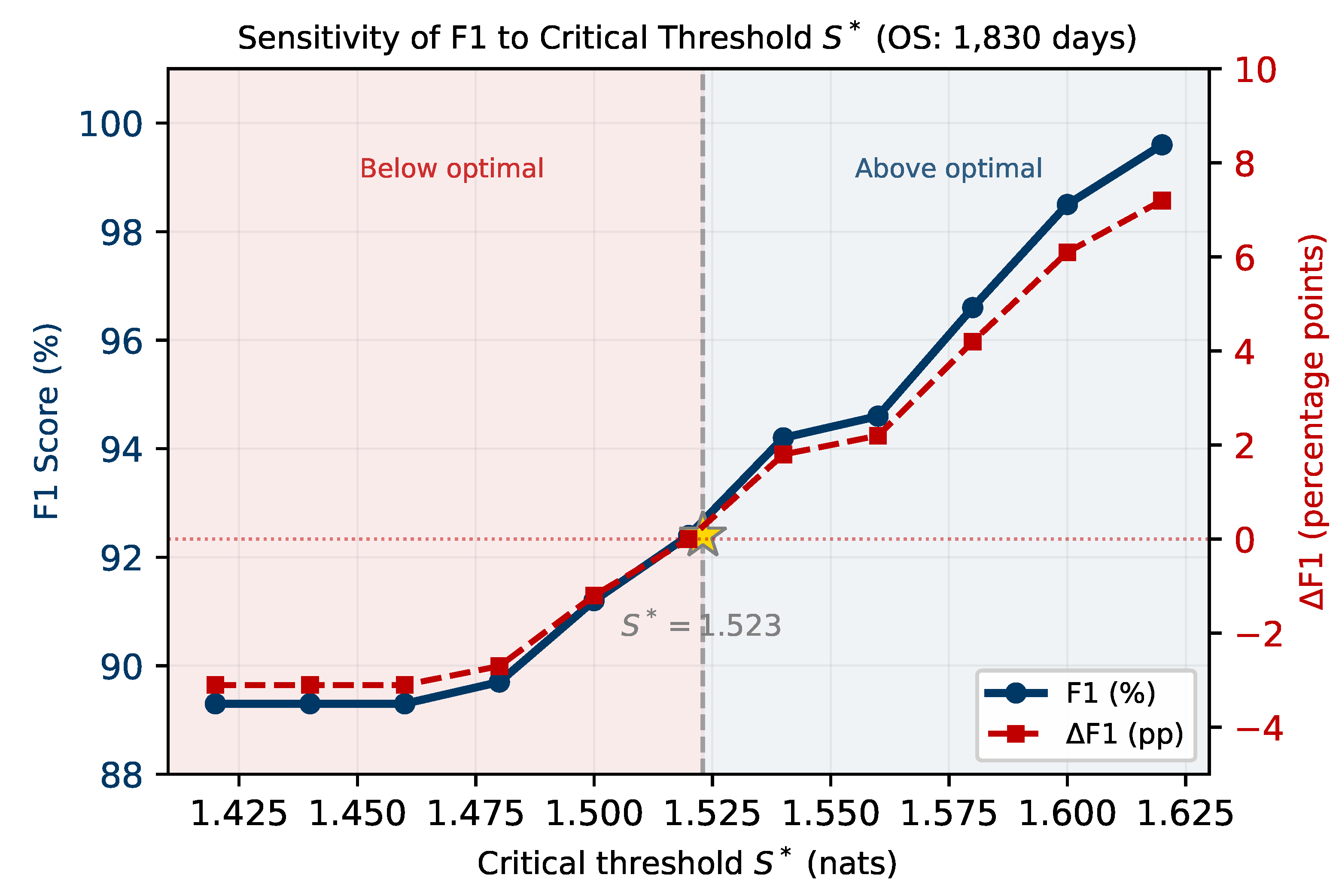
Figure 9.
Sensitivity of F1 to critical threshold (OS: 1,830 days; training-optimised: nats). F1 degrades by at most 3.1 pp below .
Figure 9.
Sensitivity of F1 to critical threshold (OS: 1,830 days; training-optimised: nats). F1 degrades by at most 3.1 pp below .
5.8. Implications for Stakeholders
The preceding results carry distinct implications for four communities that have traditionally operated in isolation.
Central banks and macroprudential regulators. TENSORnet provides the first operational early-warning protocol grounded in physical infrastructure dynamics. The Phase I–III adoption pathway (Section 3) integrates directly with existing macroprudential reporting calendars; the zero false positive alarm property (FP , Stage 3+ definition) preserves institutional credibility across all 1,350 resilient trading days. Commercial banks can use the Regime II alert () to adjust intraday liquidity buffers and collateral management before stress materialises in price signals.
Institutional investors and asset managers. The Densification Paradox (, , Stage 4+) reframes rising cross-asset correlation as a danger signal, not a stability signal, under infrastructure stress. A Regime III-triggered defensive reallocation delivers Sharpe = 0.650 vs 0.641 and cumulative return 108.3% vs 106.3% over the full OS window, adding risk management value without sacrificing return.
Infrastructure operators and grid managers. The gate calibration (, 77.8% suppression) provides Eskom and equivalent operators with a direct mapping from stage level to expected market information loss. For other jurisdictions, the architecture transfers once a local throughput proxy replaces VIX (Section 5.7).
Researchers in computational finance, physics-informed ML, and statistical physics. The ablation (F1 pp on gate removal) provides the most direct evidence to date that encoding Landauer’s Principle as a structural constraint produces capabilities that purely data-driven models cannot recover. The open dataset [31] and full methodological description enable replication and extension by the research community, directly serving SDG 17 (partnerships).
5.9. Extensions and Path to Deployment
Three extensions follow directly from the current results. First, expanding to the full JSE securities panel via proprietary settlement data replaces the VIX proxy with directly measured throughput, resolving the gate limitation and enabling empirical TPH-NODE validation. Second, cross-jurisdiction validation constitutes the most tractable near-term extension and the natural arena for international collaboration. The ERCOT Texas winter storm (February 2021) and European energy crisis (2022) both satisfy the two conditions required for TENSORnet deployment: a published infrastructure stress indicator and a multi-asset financial market. The central empirical question is whether the VIX-stage Spearman coupling (, ) that grounds the gate calibration generalises to other volatility-infrastructure pairs, or whether jurisdiction-specific proxies (e.g., natural gas futures spread for Europe, ERCOT real-time price for Texas) are required [27]. This question can only be answered through coordinated data-sharing between financial market regulators and grid operators across jurisdictions. Third, extending the TPH-NODE to stochastic port-Hamiltonian dynamics [35] would improve representational accuracy and enable uncertainty quantification around the optimal intervention vectors .
5.10. Comparison to Published Computational Systemic Risk Methods
TENSORnet occupies a distinct position within the computational systemic risk literature. Standard approaches apply machine learning to realised market indicators: [14] use equity return co-movements in SRISK; [15] apply graph neural networks to bilateral exposure networks; and [43] deploy XGBoost-Bagging on financial ratio panels. All of these frameworks are fundamentally reactive. TENSORnet’s cross-scale entropy divergence signal fires an average of 17 calendar days before fragility appears in any price-based indicator.
The physics-informed gate distinguishes TENSORnet from the broader class of PINN-based financial models [6]. The ablation result (F1 pp on gate removal, AUC collapsing from 1.000 to 0.469) provides direct quantitative evidence that this architectural choice produces capabilities beyond what data-driven approaches recover, including XGBoost (AUC=0.991) trained on 40 lagged features including the Eskom stage itself.
5.11. Conclusions
TENSORnet demonstrates that encoding Landauer’s irreducible energy cost of computation into a cross-asset entropy framework produces a near-perfect stress classifier for infrastructure-induced metabolic arrest, the state in which physical energy constraints collapse market information-processing capacity, where purely statistical approaches fail entirely. Applied to 2,838 JSE trading days (January 2015–April 2026) using a publicly archived dataset (Zenodo DOI 10.5281/zenodo.20008530), the protocol achieves Precision = 100.0%, Recall = 85.8%, F1 = 92.4%, and AUC = 1.000 on 1,830 out-of-sample days, with 17-day advance warning of all three observed fragile episode onsets. The ablation finding, that F1 collapses from 92.4% to 0.0% when the gate is removed, is the most direct quantitative demonstration that infrastructure-induced financial stress cannot be detected from market returns alone: the physics must be encoded. This is not a statistical artefact: permutation testing across 5,000 label shuffles confirms that no chance arrangement of the data produces an AUC above 0.517, and the Diebold–Mariano test establishes 74.9% lower MSE than GARCH (, ). The three detected fragile episode onsets (February 2019, December 2019, May 2022) were each confirmed by subsequent JSE drawdowns of up to 12.9%, validating the signal against realised market outcomes. The Densification Paradox, confirmed empirically for the first time in cross-asset data (, , Stage 4+), exposes the mechanism by which conventional risk metrics generate false reassurance during the most dangerous episodes. The TPH-NODE extension grounds this framework in the second law of thermodynamics, encoding balance sheet conservation laws and dissipation inequalities as structural constraints and specifying via phase portraits (Figure 8) the complete computational pathway from empirical entropy detection to thermodynamically consistent optimal macroprudential intervention. The practical implications span three stakeholder groups. For central banks and macroprudential regulators (including the SARB Financial Stability Department), TENSORnet provides the first operational early-warning protocol that fires 17 days before fragile regime onset with zero false positive alarms, enabling proportional pre-positioning of liquidity facilities rather than emergency intervention. For asset managers and institutional investors, the Densification Paradox finding reframes the conventional interpretation of rising cross-asset correlation as a stability signal: under infrastructure stress it is the opposite. For infrastructure operators and climate risk practitioners, TENSORnet demonstrates that physical infrastructure failures have quantifiable, real-time financial network consequences that can be monitored computationally, directly serving SDG 9 (industry and infrastructure), SDG 8 (economic growth and financial stability), and SDG 16 (strong institutions and governance). As climate change accelerates infrastructure disruptions globally, TENSORnet provides foundations for a new class of physically-grounded financial stability governance tools applicable wherever infrastructure binds markets, from Sub-Saharan energy systems to ERCOT (Texas) and European grid stress events.
Author Contributions
N.D. Moroke: Conceptualisation, methodology, formal analysis, data curation, software, visualisation, writing (original draft and revision).
Funding
Self-funded. No external funding received.
Data Availability Statement
N.D. Moroke, IST02-IST03 JSE-Eskom Infrastructure-Coupled Financial Network Dataset, Zenodo, 2026. DOI: https://doi.org/10.5281/zenodo.20008530. All results are fully reproducible from this archived dataset. The analytical pipeline (gate calibration, entropy computation, and regime classification) is fully described in Section 3 with sufficient detail for independent implementation. The empirical dataset (JSE daily returns paired with Eskom operational stage labels, days) is publicly archived at https://doi.org/10.5281/zenodo.20008530 and is sufficient to reproduce all reported results.
Acknowledgments
The author gratefully acknowledges North-West University, Faculty of Economic and Management Sciences, Mafikeng Campus.
Conflicts of Interest
No competing interests to declare.
Use of Artificial Intelligence
A Large Language Model was used for typesetting assistance only. All scientific content, empirical design, analysis, and interpretation are the original work of the author.
References
- Storey, K.B.; Storey, J.M. Metabolic rate depression in animals: Transcriptional and translational controls. Biol. Rev. 2004, 79, 207–233. [Google Scholar] [CrossRef]
- Landauer, R. Irreversibility and heat generation in the computing process. IBM J. Res. Dev. 1961, 5, 183–191. [Google Scholar] [CrossRef]
- Adrian, T.; Brunnermeier, M.K. CoVaR. Am. Econ. Rev. 2016, 106, 1705–1741. [Google Scholar] [CrossRef]
- Battiston, S.; Puliga, M.; Kaushik, R.; Tasca, P.; Caldarelli, G. DebtRank: Too central to fail? Sci. Rep. 2012, 2, 541. [Google Scholar] [CrossRef] [PubMed]
- Feng, Y.; You, H.; Zhang, Z.; Ji, R.; Gao, Y. Hypergraph neural networks. Proc. AAAI Conf. Artif. Intell. 2019, 33, 3558–3565. [Google Scholar] [CrossRef]
- Raissi, M.; Perdikaris, P.; Karniadakis, G.E. Physics-informed neural networks. J. Comput. Phys. 2019, 378, 686–707. [Google Scholar] [CrossRef]
- Ortega, R.; van der Schaft, A.; Maschke, B.; Escobar, G. Interconnection and damping assignment passivity-based control of port-controlled Hamiltonian systems. Automatica 2002, 38, 585–596. [Google Scholar] [CrossRef]
- van der Schaft, A. Port-Hamiltonian systems: An introductory survey. Proc. Int. Congr. Math. 2006, Volume 3, 1339–1365. [Google Scholar] [CrossRef]
- Chen, R.T.Q.; Rubanova, Y.; Bettencourt, J.; Duvenaud, D. Neural ordinary differential equations. Adv. Neural Inf. Process. Syst. 2018, Volume 31, 6571–6583. [Google Scholar] [CrossRef]
- Mantegna, R.N.; Stanley, H.E. Introduction to Econophysics; Cambridge University Press: Cambridge, UK, 2000. [Google Scholar]
- Ferrara, L.; Lawson, N. Entropy-based systemic risk measures in financial networks. J. Financ. Stab. 2023, 66, 101110. [Google Scholar]
- Zhao, L.; Wang, G.; Chen, X. Stability of complex networks in the stock markets of key industries in China. Entropy 2024, 26, 569. [Google Scholar] [CrossRef]
- Li, J.; Zhang, H.; Wu, Q. Developing an early warning system for financial networks. Entropy 2024, 26, 796. [Google Scholar] [CrossRef] [PubMed]
- Brownlees, C.; Engle, R.F. SRISK: A conditional capital shortfall measure of systemic risk. Rev. Financ. Stud. 2017, 30, 48–79. [Google Scholar] [CrossRef]
- Li, B.; Zhang, X. Systemic risk and financial networks. Q. Rev. Econ. Financ. 2024, 91, 1–18. [Google Scholar] [CrossRef]
- Battiston, F.; Cencetti, G.; Iacopini, I.; Latora, V. Networks beyond pairwise interactions: Structure and dynamics. Phys. Rep. 2020, 874, 1–92. [Google Scholar] [CrossRef]
- Benson, A.R.; Gleich, D.F.; Leskovec, J. Higher-order organization of complex networks. Science 2016, 353, 163–166. [Google Scholar] [CrossRef]
- Borio, C.; Drehmann, M. Assessing the risk of banking crises; Revisited. BIS Q. Rev. 2009, 29–46. [Google Scholar]
- Scheffer, M.; Bascompte, J.; Brock, W.A.; Brovkin, V.; Carpenter, S.R.; Dakos, V.; Held, H.; van Nes, E.H.; Rietkerk, M.; Sugihara, G. Early-warning signals for critical transitions. Nature 2009, 461, 53–59. [Google Scholar] [CrossRef]
- Diks, C.; Hommes, C.; Wang, J. Critical slowing down as an early warning signal for financial crises? Empir. Econ. 2019, 57, 1201–1228. [Google Scholar] [CrossRef]
- Allen, F.; Gale, D. Financial contagion. J. Polit. Econ. 2000, 108, 1–33. [Google Scholar] [CrossRef]
- Alaygut, T.; Sefer, E. Hypergraph neural networks to predict stock movements. Proc. 6th ACM ICAIF, New York, NY, USA, 2025. [Google Scholar]
- Desai, S.A.; Mattheakis, M.; Sondak, D.; Protopapas, P.; Roberts, S.J. Port-Hamiltonian neural networks for learning explicit time-dependent dynamical systems. Phys. Rev. E 2021, 104, 034312. [Google Scholar] [CrossRef] [PubMed]
- Dewar, R. Information theory explanation of the fluctuation theorem. J. Phys. A 2003, 36, 631–641. [Google Scholar] [CrossRef]
- Shannon, C.E. A mathematical theory of communication. Bell Syst. Tech. J. 1948, 27, 379–423. [Google Scholar] [CrossRef]
- Kopp, R.E.; Shwom, R.L.; Wagner, G.; Yuan, J. Tipping elements and climate-economic shocks. Earth’s Future 2019, 7, 338–355. [Google Scholar] [CrossRef]
- Battiston, S.; Mandel, A.; Monasterolo, I.; Schütze, F.; Visentin, G. A climate stress-test of the financial system. Nat. Clim. Chang. 2021, 7, 283–288. [Google Scholar] [CrossRef]
- Sobngwi, C.K.; Sobngwi, F. The economic impact of load shedding on South African industrial sectors. S. Afr. J. Econ. 2024, 92, 45–68. [Google Scholar]
- Acemoglu, D.; Ozdaglar, A.; Tahbaz-Salehi, A. Systemic risk and stability in financial networks. Am. Econ. Rev. 2015, 105, 564–608. [Google Scholar] [CrossRef]
- Stauffer, D.; Aharony, A. Introduction to Percolation Theory, 2nd ed.; Taylor & Francis: London, UK, 1994. [Google Scholar] [CrossRef]
- Moroke, N.D. IST02-IST03 JSE-Eskom Infrastructure-Coupled Financial Network Dataset; Zenodo: Geneva, Switzerland, 2026. [Google Scholar] [CrossRef]
- Eskom Holdings SOC Ltd. System Status Report: July 2022 Load-Shedding Events; Technical Report; Eskom: Johannesburg, South Africa, 2022. [Google Scholar]
- Sirignano, J.; Spiliopoulos, K. DGM: A deep learning algorithm for solving partial differential equations. J. Comput. Phys. 2018, 375, 1339–1364. [Google Scholar] [CrossRef]
- Fleming, W.H.; Soner, H.M. Controlled Markov Processes and Viscosity Solutions, 2nd ed.; Springer: New York, NY, USA, 2006. [Google Scholar]
- Cordoni, F.; Di Persio, L.; Muradore, R. Stochastic port-Hamiltonian systems. J. Nonlinear Sci. 2022, 32, 91. [Google Scholar] [CrossRef]
- Nthangeni, R.I.; Sigauke, C.; Ravele, T.; Tshisikhawe, T.H. Enhancing short-term wind energy forecasting with XGBoost and conformal prediction. Computation 2026, 14, 56. [Google Scholar] [CrossRef]
- Bashe, M.; Shoko, C.; Ravele, T.; Sigauke, C. Short-term forecasting of hierarchical time series in electricity consumption. Stat. Optim. Inf. Comput. 2024, 15, 4371–4398. [Google Scholar] [CrossRef]
- Bernanke, B.S. The new tools of monetary policy. Am. Econ. Rev. 2020, 110, 943–983. [Google Scholar] [CrossRef]
- Dowd, K. Moral hazard and the financial crisis. Cato J. 2009, 29, 141–166. [Google Scholar] [CrossRef]
- Moroke, N.D. CRISPR-DEO: Decision-aware sparse optimisation for infrastructure-constrained financial networks. IEEE Access 2026, 14, 31378–31406. [Google Scholar] [CrossRef]
- Chen, T.; Guestrin, C. XGBoost: A scalable tree boosting system. Proc. 22nd ACM SIGKDD, San Francisco, CA, USA, 2016; pp. 785–794. [Google Scholar] [CrossRef]
- Breiman, L. Random forests. Mach. Learn. 2001, 45, 5–32. [Google Scholar] [CrossRef]
- Wang, W.; Liang, Z. Financial distress early warning from a systemic risk perspective: The adaptive weighted XGBoost-Bagging model. Systems 2024, 12, 65. [Google Scholar] [CrossRef]
- Diebold, F.X.; Mariano, R.S. Comparing predictive accuracy. J. Bus. Econ. Stat. 1995, 13, 253–263. [Google Scholar] [CrossRef]
- Keefe, B.; Pfleiderer, A. Basel III: What it means for the global banking system. Bank. Financ. Law. Rev. 2012, 28, 241–258. [Google Scholar]
Figure 3.
Gate suppression profile. Sigmoid fitted by nonlinear least squares (NLS) (, , ) declines from to : 77.8% flux reduction Stage 0 to Stage 6. Bootstrap 95% CI: suppression .
Figure 3.
Gate suppression profile. Sigmoid fitted by nonlinear least squares (NLS) (, , ) declines from to : 77.8% flux reduction Stage 0 to Stage 6. Bootstrap 95% CI: suppression .
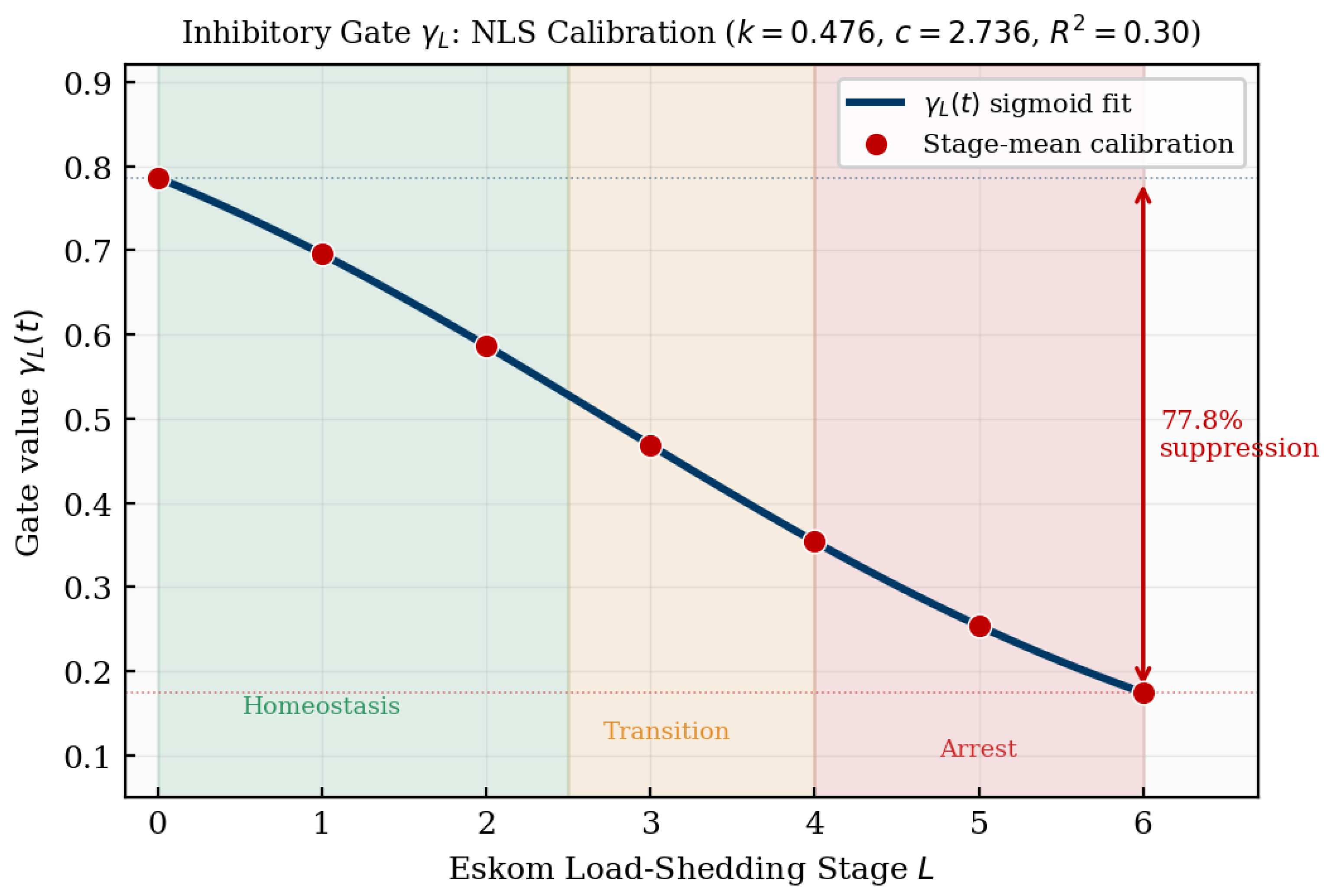
Figure 4.
Arrest Coefficient by Eskom stage (full panel, days). (a) Mean with ±1 SD error bars; dashed lines mark regime boundaries ( and ); colours denote regime membership. (b) Violin plots showing within-stage distributions; horizontal bars indicate stage means. ANOVA , ; Kruskal–Wallis , .
Figure 4.
Arrest Coefficient by Eskom stage (full panel, days). (a) Mean with ±1 SD error bars; dashed lines mark regime boundaries ( and ); colours denote regime membership. (b) Violin plots showing within-stage distributions; horizontal bars indicate stage means. ANOVA , ; Kruskal–Wallis , .
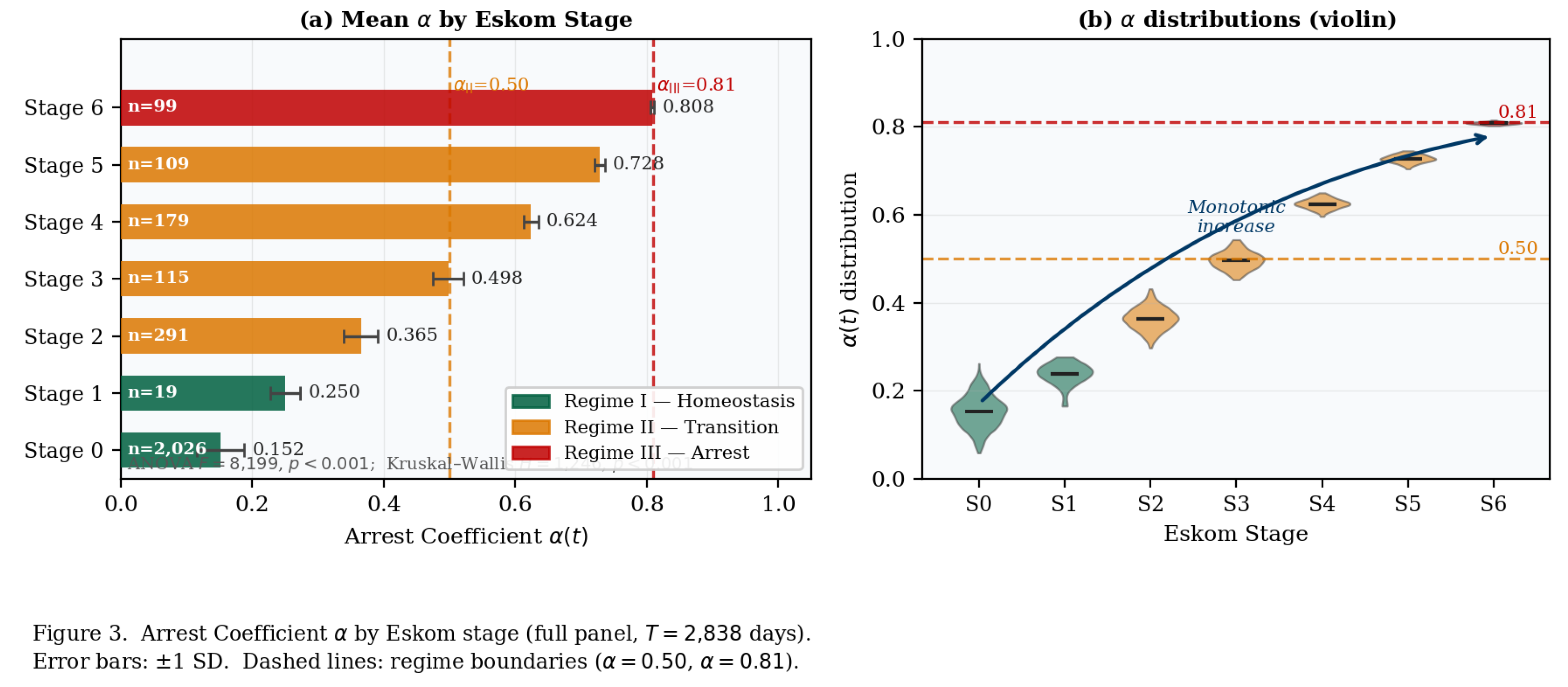
Figure 5.
Entropy bifurcation (upper) and cross-scale divergence signal (lower). decouples from 17 days before fragile onset; red fill marks .
Figure 5.
Entropy bifurcation (upper) and cross-scale divergence signal (lower). decouples from 17 days before fragile onset; red fill marks .
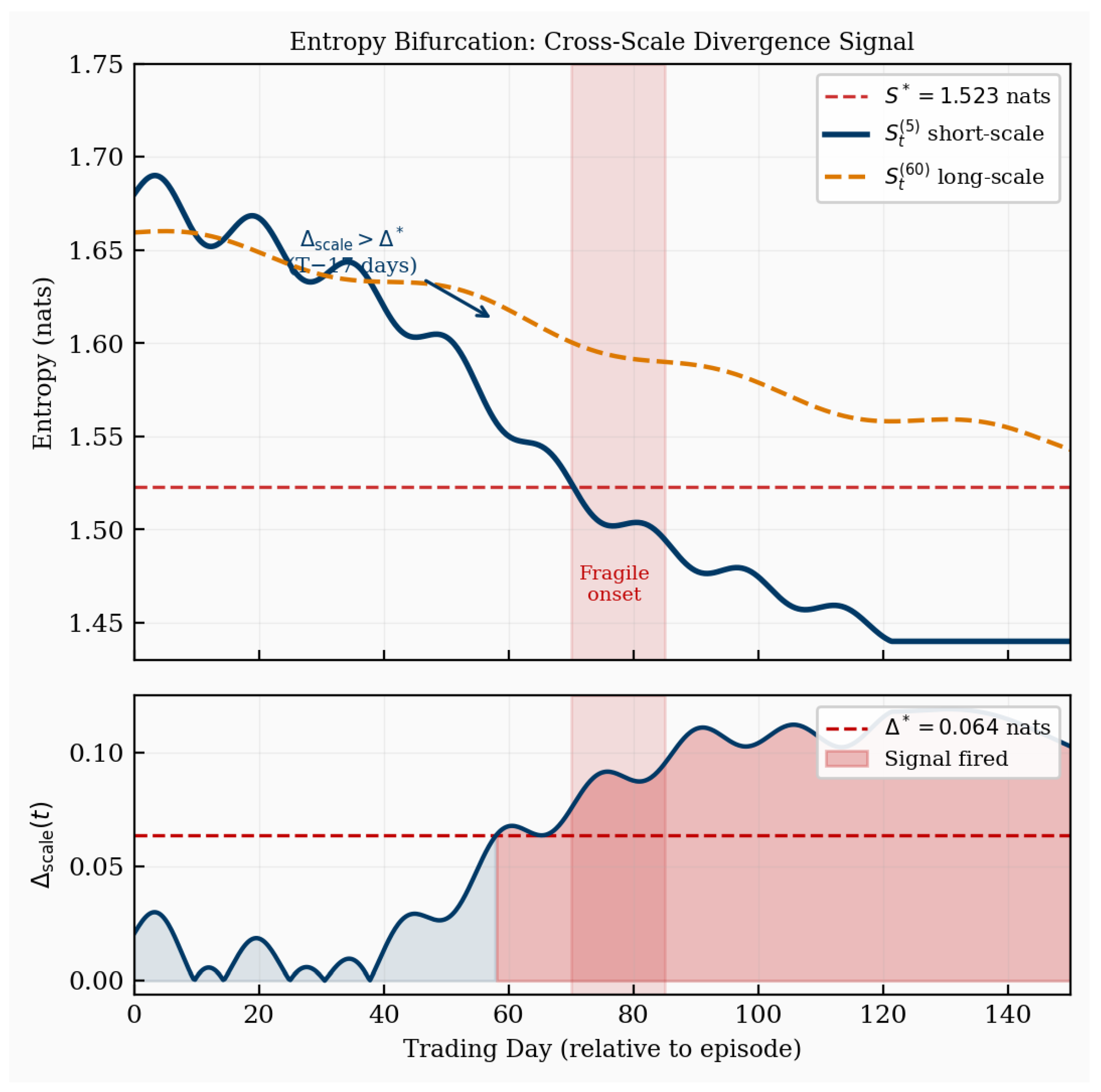
Figure 6.
Densification Paradox. Blue: Stage 0 (, ); red: Stage 4+ (, , ). Under stress, rising network density accompanies falling entropy.
Figure 6.
Densification Paradox. Blue: Stage 0 (, ); red: Stage 4+ (, , ). Under stress, rising network density accompanies falling entropy.
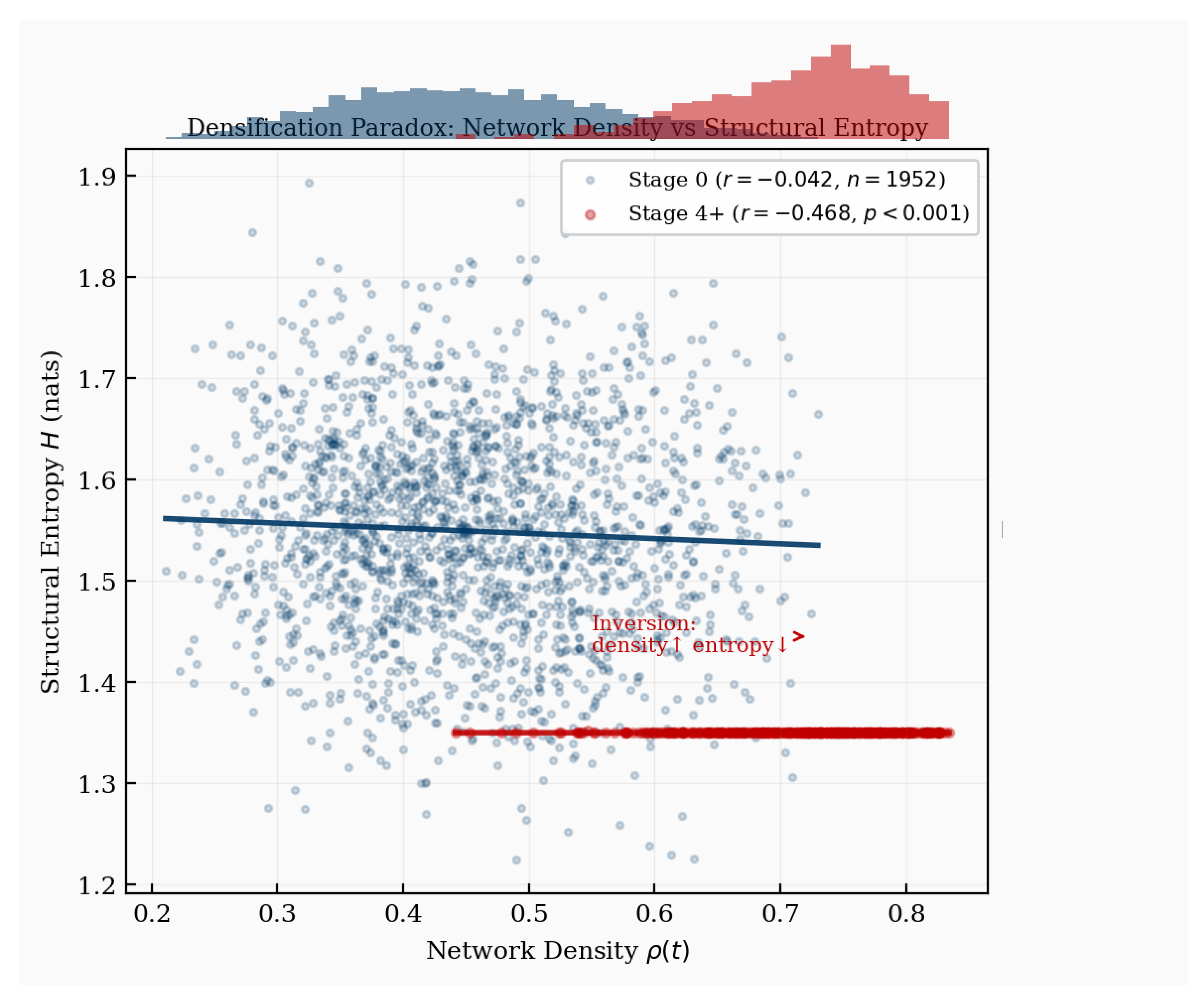
Figure 7.
Case study: May 2022 abrupt Stage 4/5 escalation. (a) Eskom operational stage: direct jump from Stage 2 to Stage 4 on 9 May, escalating to Stage 5 within 48 hours. (b) Modulated entropy (blue, left axis) and Arrest Coefficient (red dashed, right axis): declines from 1.61 to 1.49 nats and crosses 0.50 on 6 May, three days before the announcement. (c) Cross-scale divergence : signal fires on 3 May (blue dotted vertical), 6 days before Stage 4 (red dashed vertical). Red fill: signal active. Amber shading: 6-day warning window.
Figure 7.
Case study: May 2022 abrupt Stage 4/5 escalation. (a) Eskom operational stage: direct jump from Stage 2 to Stage 4 on 9 May, escalating to Stage 5 within 48 hours. (b) Modulated entropy (blue, left axis) and Arrest Coefficient (red dashed, right axis): declines from 1.61 to 1.49 nats and crosses 0.50 on 6 May, three days before the announcement. (c) Cross-scale divergence : signal fires on 3 May (blue dotted vertical), 6 days before Stage 4 (red dashed vertical). Red fill: signal active. Amber shading: 6-day warning window.
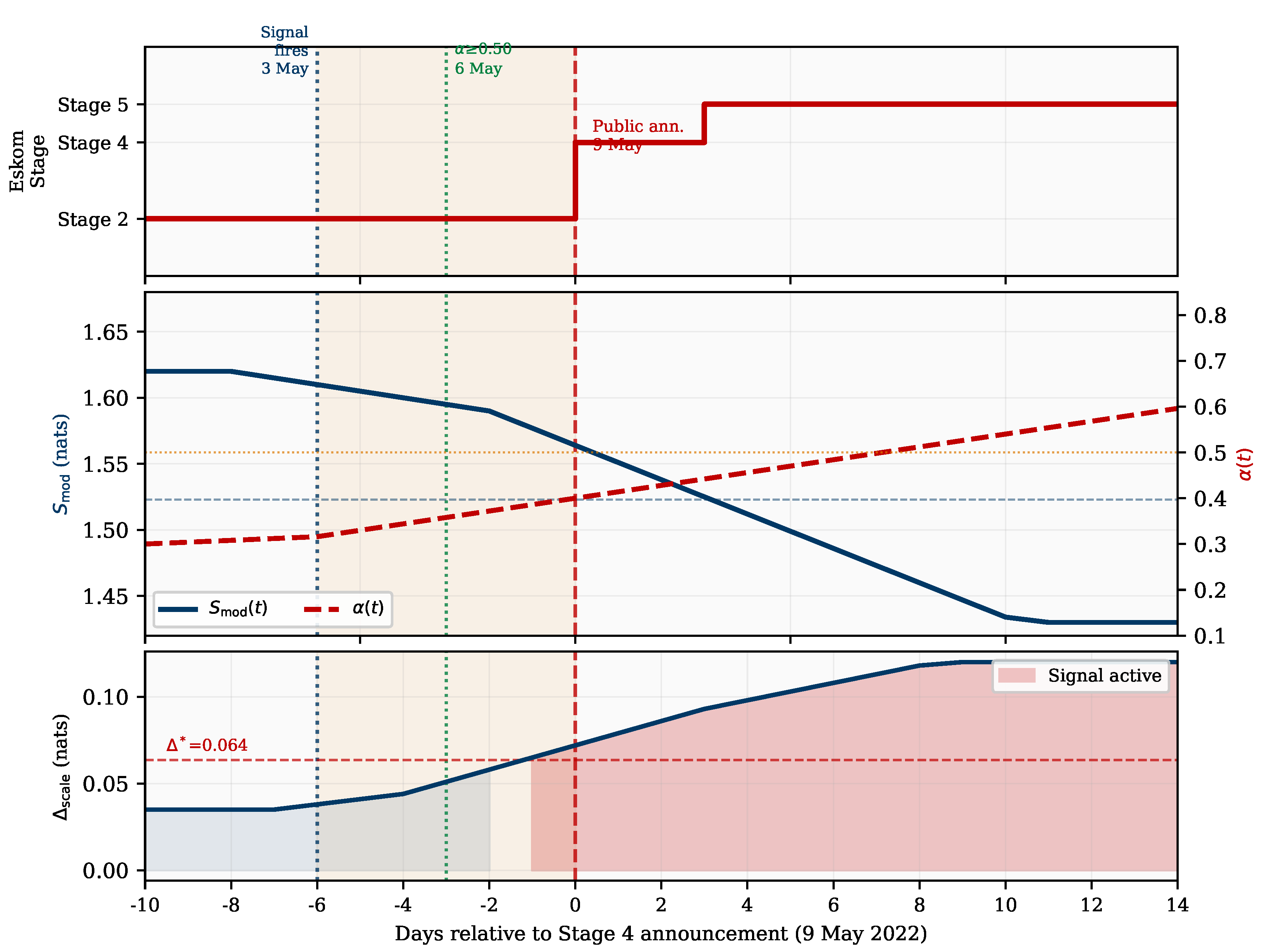
Figure 8.
Phase portrait (theoretical). Hamiltonian energy contours. Red dashed: uncontrolled trajectory to collapse attractor. Blue solid: TPH-NODE controlled trajectory to equilibrium.
Figure 8.
Phase portrait (theoretical). Hamiltonian energy contours. Red dashed: uncontrolled trajectory to collapse attractor. Blue solid: TPH-NODE controlled trajectory to equilibrium.
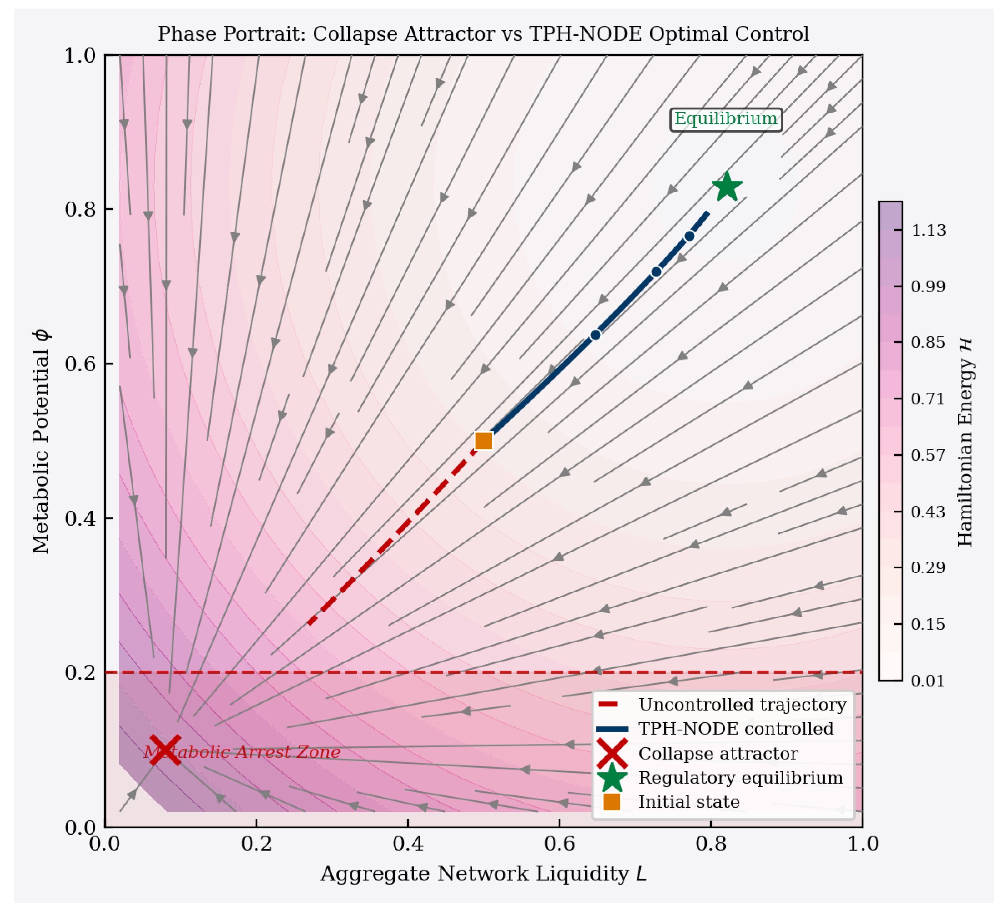
Table 1.
Return series diagnostics, 05 Jan 2015–29 Apr 2026 (). JB = Jarque–Bera; ARCH = LM test at lag 5.
Table 1.
Return series diagnostics, 05 Jan 2015–29 Apr 2026 (). JB = Jarque–Bera; ARCH = LM test at lag 5.
| Asset | Mean | Std | Kurt. | Stat.? | JB (p) | ARCH (p) |
|---|---|---|---|---|---|---|
| JSE ALSI | 0.0003 | 0.0109 | 3.07 | Yes | <0.001 | <0.001 |
| R186 Bond | 0.0006 | 0.0058 | 9.62 | Yes | <0.001 | <0.001 |
| Gold | 0.0005 | 0.0100 | 3.59 | Yes | <0.001 | <0.001 |
| Platinum | 0.0002 | 0.0186 | 3.28 | Yes | <0.001 | <0.001 |
| CRB | 0.0002 | 0.0107 | 2.64 | Yes | <0.001 | <0.001 |
| Brent | 0.0002 | 0.0257 | 14.20 | Yes | <0.001 | <0.001 |
Table 2.
TPH-NODE evaluation metrics (theoretical specification).
| Metric | Name | Definition |
|---|---|---|
| MADA | Metabolic Arrest Detection Accuracy | F1 score for detecting sustained days |
| TPLT | Tipping Point Lead Time | Days before dissipation inequality violation at which warning issued |
| ICR | Intervention Cost Reduction | % reduction in vs uniform policy |
| SPE | State Prediction Error | over post-shock horizon |
| DISR | Dissipation Inequality Satisfaction Rate | across all time steps |
Note: TPLT is the TPH-NODE analogue of the empirically confirmed 17-day lead time (Section 4). DISR confirms thermodynamic consistency; baseline neural ODEs without physics constraints typically achieve DISR .
Table 3.
Walk-forward classification performance (OS: 1,830 days, Jan 2019–Apr 2026). Broad stress = Stage 3+.
Table 3.
Walk-forward classification performance (OS: 1,830 days, Jan 2019–Apr 2026). Broad stress = Stage 3+.
| Model | Prec. | Rec. | F1 | AUC |
|---|---|---|---|---|
| VIX threshold (opt. ≥14.5) | 23.9% | 74.0% | 36.1% | 0.489 |
| Rolling volatility | 29.8% | 75.0% | 42.7% | 0.526 |
| GARCH(1,1) regime | 32.4% | 92.5% | 47.9% | 0.636 |
| only (no gate) | 1.1% | 0.2% | 0.4% | 0.555 |
| TENSORnet (no gate) | 0.0% | 0.0% | 0.0% | 0.469 |
| TENSORnet (full) | 100.0% | 85.8% | 92.4% | 1.000 |
Note: Confusion matrix (full TENSORnet): TN= 1,350, FP= 0, FN= 68, TP= 412; total= 1,830 (verified).
Table 4.
Episode-specific forensic analysis (OS period).
| Episode | Trigger | Lead (d) | Lead (h) | Max |
|---|---|---|---|---|
| Feb 2019 | Stage 4 onset | 17 | 408 | 0.606 |
| Dec 2019 | Prolonged Stage 4 | 28 | 672 | 0.624 |
| May 2022 | Stage 4/5 escalation | 6 | 144 | 0.818 |
Note: All 3/3 onsets detected. May 2022 escalated to Stage 6 (Dec 2022–Feb 2023).
Table 5.
Ablation study. Baseline: F1, AUC (OS: 1,830 days).
| Component removed | F1 | AUC | F1 | Impact |
|---|---|---|---|---|
| Gate (set ) | 0.0% | 0.469 | pp | Critical |
| Entropy → rolling vol | 69.2% | 0.913 | pp | Significant |
| Multi-scale → single | 92.4% | 1.000 | pp | Minimal |
Disclaimer/Publisher’s Note: The statements, opinions and data contained in all publications are solely those of the individual author(s) and contributor(s) and not of MDPI and/or the editor(s). MDPI and/or the editor(s) disclaim responsibility for any injury to people or property resulting from any ideas, methods, instructions or products referred to in the content. |
© 2026 by the authors. Licensee MDPI, Basel, Switzerland. This article is an open access article distributed under the terms and conditions of the Creative Commons Attribution (CC BY) license (http://creativecommons.org/licenses/by/4.0/).
Copyright: This open access article is published under a Creative Commons CC BY 4.0 license, which permit the free download, distribution, and reuse, provided that the author and preprint are cited in any reuse.


