
Submitted:
17 May 2026
Posted:
19 May 2026
You are already at the latest version
Abstract
The impact of jawbone diseases extends far beyond the mouth. Worldwide, cancer patients completing chemotherapy often have routine dental checkups, with about 70% of patients with breast and prostate cancer and 30–40% of those with lung and other solid tumours being diagnosed with bone metastases. Oncologists treating these patients usually prescribe bisphosphonates to protect their bones, a common and necessary treatment. Yet determining whether the jawbone is starting to deteriorate is something neither the patient nor the dentist can easily detect. Studies show that medication-related osteonecrosis of the jaw (MRONJ) affects a growing share of the millions of patients on antiresorptive therapies across Egypt, the Gulf, and North Africa (up to 15%, compared to just 0.01% in the general population). Nevertheless, by the time it becomes clinically visible, the bone damage is often already irrecoverable. Patients recovering from head and neck radiotherapy, elderly patients with chronic bone loss, and those living with metabolic bone disorders face the same invisible progression. Moreover, all experience the same diagnostic gap, as the primary imaging tool, CBCT, has major drawbacks: its interpretation relies heavily on visual inspection, making conclusions highly subjective, along with the shortage of specialists in many areas, causing patients’ conditions to deteriorate between visits. Globally, more than 12.5 million Cone Beam Computed Tomography (CBCT) scans are performed annually, with total imaging volume increasing by over 50% in the last five years. Additionally, in the Middle East and Africa alone, the CBCT imaging market is projected to grow at a compound annual rate of 12.91% through 2032. This growth creates an expanding diagnostic workload that current practices are unable to meet, highlighting the need for new automated and reliable imaging models. In this work, we propose AutoCBCT, an automated CBCT model that combines Attention U-Net segmentation — which learns to focus on anatomically relevant structures while ignoring noise — with Euclidean Distance Transform-based thickness mapping to produce a spatial heatmap of the entire jaw. Indicators for MRONJ, osteoradionecrosis, fibrous dysplasia, and resorption are based on established clinical criteria. The proposed framework serves as a support tool for clinical decision-making through resorption grading (based on the Cawood and Howell classification) and automated detection of abnormal bone density patterns. The proposed approach is evaluated using 443 CBCT scans from the ToothFairy international dataset, obtained from three commercial scanner platforms with voxel spacings of 0.160–0.300 mm. Bone segmentation achieved a mean Dice coefficient of 0.884 ± 0.020 (range 0.798–0.938), with all 443 cases exceeding the clinical acceptance threshold of 0.7. The thickness estimation of the bone showed a mean absolute error of 0.209 ± 0.094 mm, with 99% of patients below 0.5 mm and every patient below 1.0 mm. The total mean thickness of the bone was 2.797 ±0.410 mm. The clinical data showed that 73.6% of the patients required augmentation or reconstruction. There was no abnormal bone in this dataset.
Keywords:
jawbone disease detection
; CBCT
; attention U-Net
; bone thickness
; deep learning
; medical diagnostics
1. Introduction
Aging, pharmacological interventions, and radiation exposure are key systemic influences that remodel the biologically active tissue known as the jawbone. Unless jawbone problems are detected early, progressive bone deterioration may occur, often resulting in significant functional complications. On the other hand, current imaging tools used to detect subtle structural and density alterations pose a challenge, as it is difficult to accurately identify bone problems visually using the human eye and subjective diagnosis.
Cone Beam Computed Tomography (CBCT) is widely used in the Middle East and North Africa (MENA) region to evaluate jawbone condition. However, CBCT interpretation is generally qualitative, relying on visual inspection and subjective estimation by clinicians. This visually-based inspection approach results in inconsistent conclusions among different specialists making many results unreliable and incapable of detecting small-scale changes.
Several clinically significant conditions illustrate these limitations. For example,progressive alveolar bone loss following tooth extraction, affects a substantial portion of the estimated 2.3 billion individuals worldwide experiencing tooth loss , [1]. Medication-related osteonecrosis of the jaw (MRONJ), which is associated with bisphosphonates is increasingly observed in aging populations and oncology patients receiving long term therapy [2]. Altohugh early stages of MRONJ often present changes in bone density, such changes are often not readily identified during routine CBCT review. Similarly, progressive osseous deterioration is common in up to 15% of patients treated with head and neck radiotherapy, this deterioration pregresses silently until advanced disease stages are encountered [3]. Finally, abnormal and asymmetric jawbone remodeling that occurs in patients with metabolic bone disorders require careful monitoring and diagnosis [4].
All these conditions, although common and widely spread in large number of patients, do suffer from the lack of quantitative, reliable metrics within the standard CBCT workflow. Currently, scans’ results are subjective evaluations, lacking standardized numerical benchmarks or reliable baseline comparisons. Consequently, diagnostic decisions remain dependent on human interpretations and visual observations This diagnostic gap highlights an urgent need for an automated, measurement-driven approaches to jawbone assessment. The rest of this paper presents a novel quantitative, deep learing-based framework that aims to close this gap through providing a reliable, cost-efficient model that can support clinical decision-makers to early detect jawbone problems and consequently increase the chances of recovery
2. Proposed Model: A Deep Learning-Based Bone Disease Assessment Model
2.1. System Architecture Overview
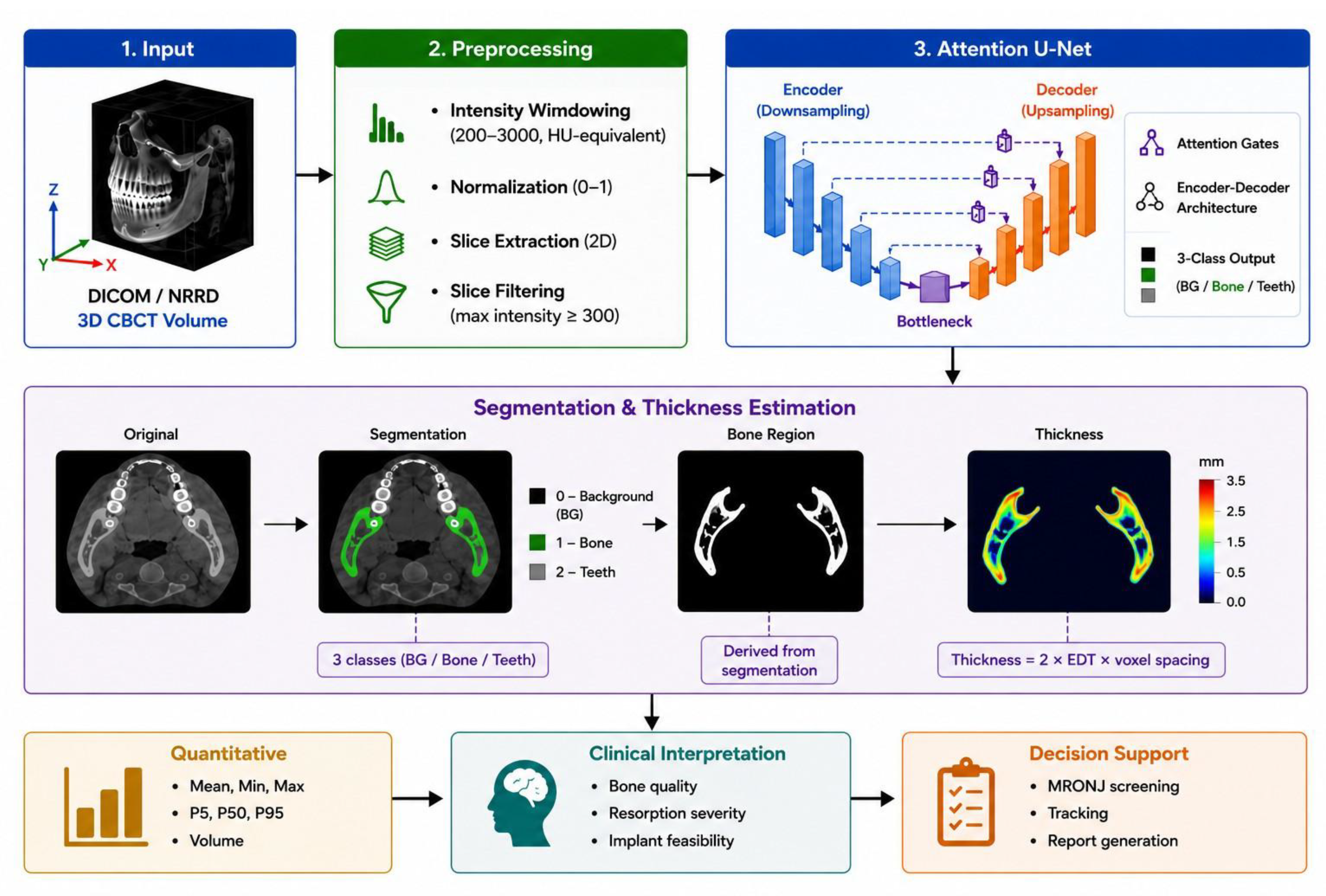
The proposed Auto-CBCT Bone Thickness Analyzer framework is designed as a modular pipeline that converts raw CBCT scans into quantitative assessments of jawbone structure. The framework architecture consists of four main phases: (1) data ingestion and preprocessing, (2) deep learning–based segmentation, (3) geometric thickness estimation, and (4) feature extraction and disease-oriented analysis. The main characteristic of the proposed framework is its capability to analyze standard clinical imaging format and its robustness to variations in scanner characteristics.
Figure 1.
Overview of the AutoCBCT pipeline.
2.2. Phase 1: Data Ingestion and Preprocessing
Patient volumes are stored as three-dimensional arrays loaded directly from disk. The preprocessing pipeline runs on each axial slice, applying a series of steps to standardize inputs across heterogeneous acquisition conditions. Slices are first screened for clinical content before processing. Before processing, each slice is checked for clinical content. Axial slices with a maximum Hounsfield Unit value of less than 300 HU are rejected because they contain no bone signal and will only contribute background noise during training. Slices that are fully background after label generation are also excluded. This filtering reduces the overall volume of training data while guaranteeing that the remaining slices include anatomically relevant content.
Segmentation labels are generated from the retained slices using HU thresholding. The bone class includes both cortical and cancellous tissue, with voxels ranging from 300–2200 HU. Voxels with HU values above 2200 and up to 5000 are classified as teeth, which include enamel and high-density restorations. All remaining voxels are treated as background. The labeling system with three classes (background, bone, and teeth) represents the segmentation targets necessary for downstream thickness estimate and disease classification.
In this phase, each slice is resized to a uniform spatial dimension using bilinear interpolation for image data and nearest-neighbor interpolation for masks. The proposed approach keeps label values complete without blending at the pixel level. The intensity values are then clipped to the range [200,3000] HU and normalized to fall within [0,1] as shown in Equation (1) [17].

This range was chosen to cover the full variety of jawbone tissue types. It includes low- density cancellous bone at the lower end and dense enamel and metal restorations at the upper end, while limiting the impact of air and soft tissue. Processed images are stored as 32-bit floating-point arrays, and masks are stored as 8-bit unsigned integers.
As for the dataset, we made an 80/20 split for training and validation, respectively, before any of this processing took place. It is important to divide at the patient level rather than by the slice; this avoids having slices from the same person in both sets. This prevents the inflated performance estimates that would occur from slice-level leakage. The split was done using a fixed random seed to make sure the process can be repeated. Figure 1 shows the proposed CBCT-based bone thickness analysis pipeline.
2.3. Phase 2: Jawbone Segmentation with Attention U-Net
AutoCBCT uses the Attention U-Net architecture for segmenting the jawbone. The network follows an encoder–decoder structure, where the encoder progressively captures contextual features and the decoder reconstructs spatial detail. Attention gates are employed to selectively highlight anatomically relevant regions, allowing the model to focus on bone structures and ignore background noise and artefacts.
The model is trained to produce multi-class segmentation outputs, distinguishing between background, total bone (including cortical and cancellous components), and teeth. This approach reflects clinical practice, where decisions depend mainly on total bone volume rather than detailed tissue composition.
2.4. Phase 3: Geometric Bone Thickness Estimation
Following the segmentation phase, quantitative assessment of bone structure is achieved through geometric thickness estimation. For each segmented bone mask, the Euclidean Distance Transform (EDT) is computed to determine the shortest distance from each voxel to the nearest boundary [16]. Local thickness is estimated as twice the radius of the maximal inscribed sphere at each voxel, approximated via the Euclidean Distance Transform and scaled by voxel spacing as shown in Equation (2) [15]. The main volume-level statistics include mean, P5, P50, and P95, which serve as quantitative inputs to the disease classification module [7].

2.5. Phase 4: Disease Classification
The disease detection module outputs are generated in alignment with clinical criteria. Abnormal density patterns are used to assess MRONJ and osteoradionecrosis risk based on mean Hounsfield Unit values outside the healthy bone range (below 800 or above 1,400 HU) combined with extreme localized thinning (P5 < 0.4 mm), thereby generating a risk indicator that alerts clinicians without replacing their clinical judgment. Meanwhile, asymmetry in thickness distribution is used to identify fibrous dysplasia and Paget-like patterns. Resorption severity is graded using the Cawood and Howell classification [11], providing a standardized, reproducible model that supports longitudinal disease monitoring.
The longitudinal monitoring capability is a major advantage of the AutoCBCT. Different patients require periodic jawbone assessment throughout their treatment often for years. Current assessment techniques rely on manual interpretation, with no objective baseline comparison. On the other hand, the proposed AutoCBCT Bone Thickness Analyzer generates quantitative biomarkers that can be tracked over time, flagging deterioration before it becomes clinically visible and providing treating treating oncologists and oral surgeons with objective, quantitative data that enables informed decisions regarding the optimal treatment plan.
3. Evaluation Results
3.1. Dataset and Evaluation Protocol
Experiments were conducted on the ToothFairy CBCT dataset [8,9,10], which comprises 443 volumetric scans collected across three commercial scanner platforms: Planmeca ProMax, Carestream CS 9300, and Sirona Galileos. Voxel spacing ranges from 0.160 to 0.300 mm in plane, with scan depths between 167 and 172 slices. This heterogeneity makes the dataset a realistic proxy for multi-site clinical deployment. Because the ToothFairy dataset provides annotations only for the mandibular canal, ground truth labels for bone and teeth were approximated using intensity-based thresholding. Voxels within the range of 300–2200 HU were assigned to the bone class, while voxels exceeding 2200 HU were classified as teeth. These thresholds are consistent with reported intensity ranges for mineralized tissues in CT and CBCT imaging, where hard tissues exhibit significantly higher density values than surrounding structures [12,13,14].
3.2. Segmentation Performance
The segmentation results for all 443 patients are shown in Table 1. Bone Dice scores ranged from 0.798 to 0.938, with a mean of 0.884 ± 0.020. This level of performance was maintained consistently across the dataset’s variation in scanner hardware and acquisition settings, as indicated by the standard deviation of 0.020. All patients exceeded the 0.7 threshold, which is commonly used as a clinical acceptance criterion in medical image segmentation.
The teeth segmentation resulted in a mean Dice of 0.789 ± 0.087, which is slightly lower and more variable than the bone result. Most of this can be due to two factors: edentulous patients, where no teeth are present in the scan volume, and metallic restorations that produce HU scatter corrupting local intensity values. Since bone thickness is the primary clinical outcome of the system, neither of these factors affects the system’s fundamental benefit.
3.3. Bone Thickness Measurement
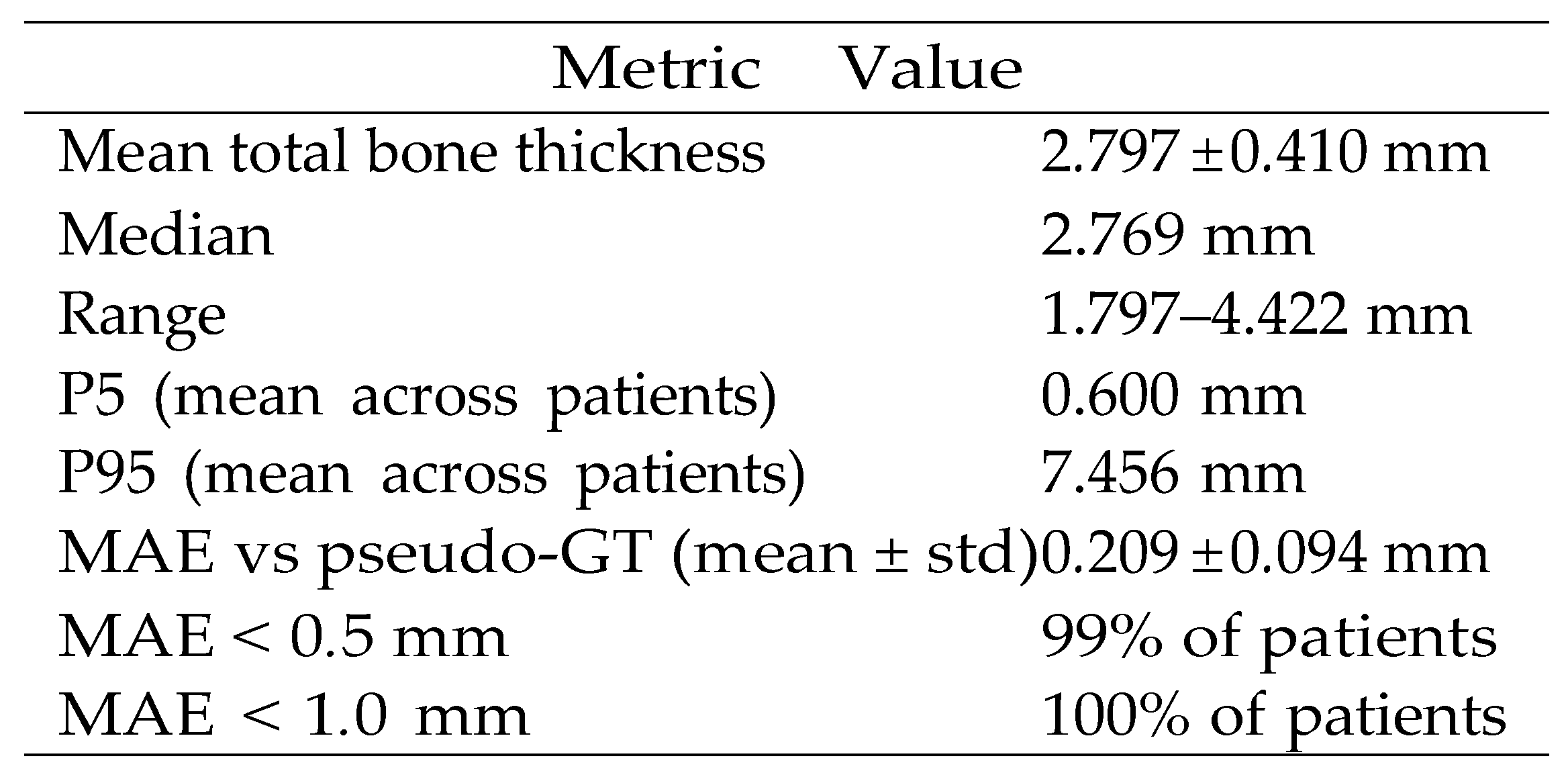
Results of the thickness estimate are presented in Table 2. It should be noted that the mean absolute error value is 0.209 ± 0.094 mm, which may be regarded as appropriate for classification tasks, especially considering that in clinical classification, distances between scores of resorption usually are at least 1.0 mm. In particular, the mean absolute error of thickness estimation per patient did not exceed 0.5 mm in 99% of cases, and the largest error of thickness estimation was less than 1.0 mm in the entire patient dataset of the current study.
Mean total bone thickness of all the 443 patients was 2.797 ± 0.410 mm, with a median of 2.769 mm. This entire range (1.797–4.422 mm) includes not only the very resorbed ridges but also the small percentage of patients with relatively preserved bone volume. The P5 value of 0.600 mm emphasizes the thin ridge regions that are clinically important for implant site selection, whereas the P95 value of 7.456 mm reflects the upper tail of patients with denser bone.

Table 2.
Bone thickness measurement results (n = 443).
 |
3.4. Bone Thickness Distribution
Figure 2 shows the distribution of the mean bone thickness values across the cohort. The distribution is approximately bell-shaped with the peaking in the 2.5–3.0 mm interval and a tail towards 4.5 mm. The large majority of patients are under the 3.0 mm reduced-bone threshold, and represent a population where the majority of patients have clinically insufficient bone for standard implant placement. A very small number of cases reach or exceed the adequate-bone threshold of 4.0 mm. Fewer than five patients exceed this value by any meaningful amount. The distribution shape is a concentration between 2.0 and 3.5 mm with very few extreme values on either side. This is broadly consistent with what one would expect from a CBCT referral population skewed towards moderate and advanced ridge resorption.
3.5. Disease Classification Results
Table 3 shows the classification results for all 443 patients. Cawood and Howell Class IV was the dominant category and included 72.5% of patients (321 out of 443). Next was Class III followed at 26.0% (115 patients), which represented those with decreased but potentially usable bone for narrow-diameter implants. Five patients (1.1%) were classified as Class V, indicating extreme resorption requiring major reconstruction. Two patients (0.5%) were classified as Class II, where bone dimensions approach the threshold for standard implant placement subject to site-level assessment. No patients achieved Class I.
Additionally, the findings reveal that 73.6% of cases require augmentation or reconstruction before the placement of dental implants. The remaining 26.4% fall under Class II or Class III and could potentially be candidates for regular or narrow implants, but only after a thorough site evaluation. None of the 443 patients triggered the MRONJ monitoring flag. The bone density measurements were all within the predicted physiological range; none of the cases exhibited the abnormal HU patterns or severe localized thinning that the screening module is intended to identify. This indicates that the detection threshold does not generate false positives at a rate that would be clinically disruptive, even though it also means that the module was not tested on positive cases in this dataset.
3.6. Segmentation Examples
Figure 3 presents segmentation outputs for four representative patients (P1–P4), demonstrating the system’s ability to delineate total jawbone tissue and generate clinically interpretable thickness heatmaps. The blue/cyan dominant values (1–2 mm) in heatmaps confirm the prevalence of moderate-to-severe bone loss across the cohort.
4. AutoCBCT Applicability and Clinical Deployment
Both the clinical usage and the deployment of the proposed system are important. A key advantage of AutoCBCT is its minimal infrastructure barrier, requiring no additional hardware and operating directly on standard clinical workstations already present in dental practices, oral surgery units, and hospital imaging departments. In addition, AutoCBCT is compatible with all major scanner manufacturers requiring no hardware replacement and making its deployment cost-effective and without any captial investment beyond the software. This low operation cost makes it accessible not only to well-resourced urban centers, but also to the district hospitals and regional clinics that serve the majority of MENA patients. Egypt, Gulf, and North Africa are regions with an increasing rate of cancer patients receiving antiresorptive or radiation who need regular CBCT scans to monitor their jawbone condition. Not to mention, elderly patients with progressive bone loss and systemic bone disease represent another group whose jawbone health is currently monitored inconsistently and subjectively. AutoCBCT’s benefit is not limited to treating individual patients, it provides a tool for generating objective, comparable, longitudinal bone assessments. The framework creates a data infrastructure that enables audit, quality assurance, research, and population-level disease monitoring for various dental services. Deploying AutoCBCT in hospitals and adopting it by dental service providers help build patient datasets that, over time, enhance the system’s performance and with clinical support enable early disease detection and effective treatment plans development.
5. Conclusions
In this paper, a deep learning framework was proposed for automated assessment of jaw bone conditions using CBCT-based bone thickness analysis. The proposed approach generate quantitative measurements that can support clinical evaluation of jawbone quality and resorption severity using the attention U-Net segmentation with geometric thickness estimation. The system was trained and evaluated using 443 CBCT scans from the ToothFairy multi scanner dataset, which includes images obtained from Planmeca ProMax, Carestream CS 9300, and Sirona Galileos scanners. The results showed demonstrated consistent performance throughout the heterogeneous dataset.
The segmentation results for bone yielded a Dice score value of 0.884±0.020, where all patients had values above the 0.7 clinical threshold, with an average Hausdorff distance of 11.10
± 3.57 mm at bone edges. The thickness measurements were estimated within 0.209 ± 0.094 mm, with 99% of the patients having errors less than 0.5 mm, which is sufficiently accurate for staging based on the Cawood and Howell system without inter-grade misclassification due to measurement errors. Clinically, the results show a cohort with significant bone loss. After a sitelevel evaluation, it was shown that about 75% of patients needed augmentation or reconstruction prior to implant placement, while the remaining 25% of patients had enough bone for at least a narrow-diameter implant. No cases presented the atypical density patterns that would warrant MRONJ referral, though this reflects the composition of the dataset rather than a claim about the screening module’s sensitivity on positive cases.
The main contribution of this work is the transition from subjective visual CBCT interpretation to repeatable quantitative evaluation, offering thickness maps and numerical measurements that help clinicians with diagnosis, implant design, and long-term monitoring without depending exclusively on manual inspection. The system generates all of this without requiring specific inference hardware, image processing knowledge, or modifications to the CBCT acquisition process. Because the system works with standard CBCT scans without requiring specialized hardware or significant workflow modifications, its demonstrated consistency across three commercial scanner platforms and a wide range of voxel spacings make it appear reliable enough for diverse clinical settings—a significant benefit that supports its potential application in real-world practice, as the system functions with standard CBCT scans without requiring specialist hardware or major workflow modifications.
References
- GBD 2019 Diseases and Injuries Collaborators. Global burden of 369 diseases and injuries, 1990–2019. Lancet 2020, 396, 1204–1222. [CrossRef] [PubMed]
- Ruggiero, S.L.; et al. AAOMS position paper on MRONJ — 2022 update. J. Oral. Maxillofac. Surg. 2022, 80, 920–943. [Google Scholar] [CrossRef] [PubMed]
- Marx, R.E. Osteoradionecrosis: A new concept of its pathophysiology. J. Oral. Maxillofac. Surg. 1983, 41, 283–288. [Google Scholar] [CrossRef] [PubMed]
- Cawood, J.I.; Howell, R.A. A classification of the edentulous jaws. Int. J. Oral. Maxillofac. Surg. 1988, 17, 232–236. [Google Scholar] [CrossRef] [PubMed]
- Oktay, O.; et al. Attention U-Net: Learning where to look for the pancreas. MIDL. 2018. [Google Scholar]
- Ronneberger, O.; Fischer, P.; Brox, T. U-Net: Convolutional networks for biomedical image segmentation. MICCAI 2015, 9351, 234–241. [Google Scholar]
- Hildebrand, T.; Ruegsegger, P. Model-independent assessment of thickness in three- dimensional images. J. Microsc. 1997, 185, 67–75. [Google Scholar] [CrossRef]
- Bolelli, F.; Lumetti, L.; Vinayahalingam, S.; Di Bartolomeo, M.; Pellacani, A.; Marchesini, K.; Grana, C. Segmenting the Inferior Alveolar Canal in CBCTs Volumes: the ToothFairy Challenge. IEEE Transactions on Medical Imaging. [CrossRef] [PubMed]
- Lumetti, L.; Pipoli, V.; Bolelli, F.; Ficarra, E.; Grana, C. Enhancing Patch-Based Learning for the Segmentation of the Mandibular Canal. IEEE Access. 2024. [Google Scholar] [CrossRef]
- Cipriano, M.; Allegretti, S.; Bolelli, F.; Pollastri, F.; Grana, C. Improving Segmentation of the Inferior Alveolar Nerve through Deep Label Propagation. In IEEE/CVF Conference on Computer Vision and Pattern Recognition (CVPR); IEEE, 2022. [Google Scholar]
- Cawood, J.I.; Howell, R.A. A classification of the edentulous jaws. Int. J. Oral. Maxillofac. Surg. 1988, 17, 232–236. [Google Scholar] [CrossRef] [PubMed]
- Kalender, W. A. Computed Tomography: Fundamentals, System Technology, Image Quality, Applications; Wiley, 2011. [Google Scholar]
- Pauwels, R. Cone beam CT for dental and maxillofacial imaging. Dentomaxillofacial Radiology. 2015. [Google Scholar]
- Kim, M. S.; Kim, J. D.; Kang, D. W. Measurement of hard tissue density of head phantom based on the HU by using CBCT. Korean J. Oral. Maxillofac. Radiol. 2009, 39, 115–120. [Google Scholar]
- Hildebrand, T.; Rüegsegger, P. A new method for the model-independent assessment of thickness in three-dimensional images. J. Microsc. 1997, 185, 67–75. [Google Scholar] [CrossRef]
- Borgefors, G. Distance transformations in digital images, Computer Vision, Graphics, and Image Processing. 1986. [Google Scholar]
- Gonzales, R.C.; Woods, R.E. Digital Image Processing, 4th ed.; Pearson, 2018. [Google Scholar]
Figure 2.
Total bone thickness distribution across 443 patients. Distribution peaks between 1.8-2.2 mm with near-complete absence above 3.0 mm (orange dashed line). Red dashed line (2.0 mm) marks severe resorption threshold. Orange dashed line (3.0 mm) marks reduced bone threshold. Green dashed line (4.0 mm) marks adequate bone — no patients reach this threshold.
Figure 2.
Total bone thickness distribution across 443 patients. Distribution peaks between 1.8-2.2 mm with near-complete absence above 3.0 mm (orange dashed line). Red dashed line (2.0 mm) marks severe resorption threshold. Orange dashed line (3.0 mm) marks reduced bone threshold. Green dashed line (4.0 mm) marks adequate bone — no patients reach this threshold.
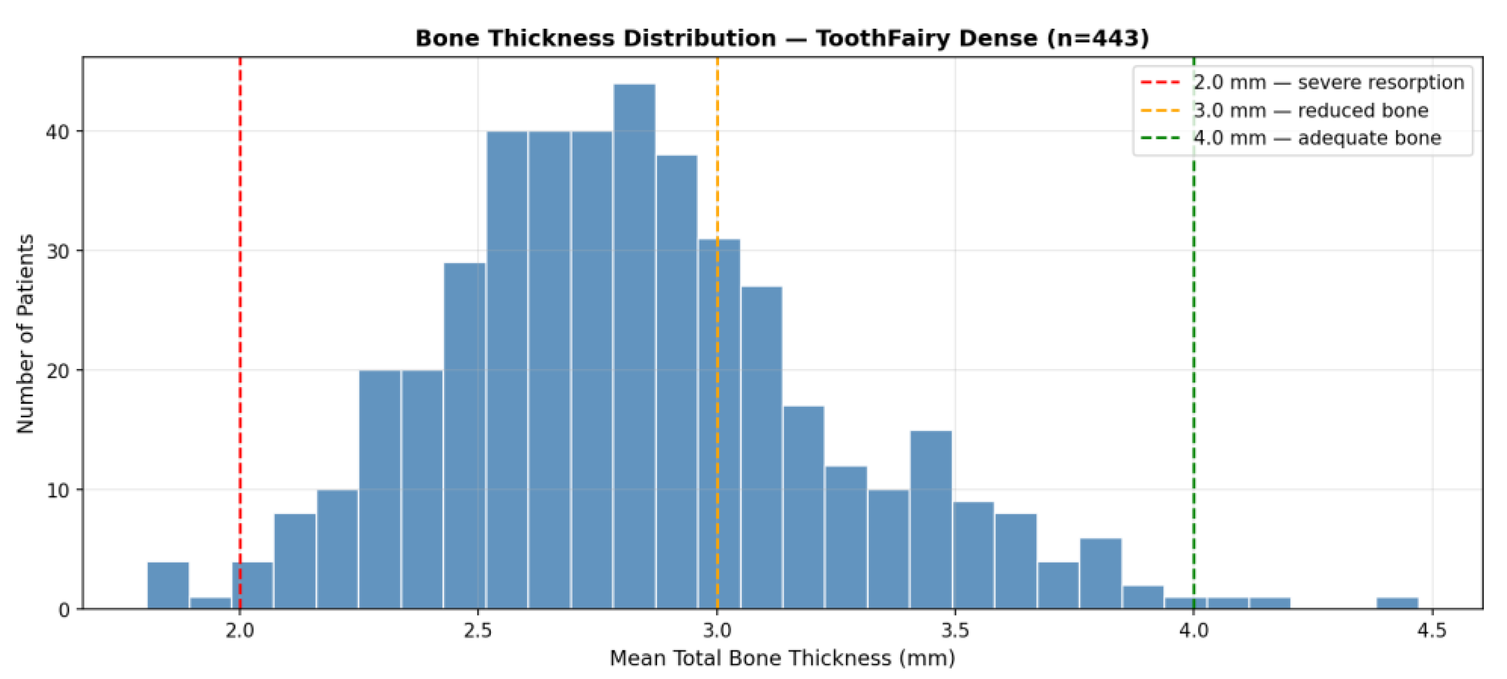
Figure 3.
Segmentation examples for four patients. Each panel shows (left to right): Original CT, Segmentation Overlay, Bone Mask, Thickness Heatmap. Color scale: 0–5 mm (blue = thin, red = thick). Note the thin blue/cyan ridges in P1 and P2 (Class V extreme resorption) versus slightly thicker but still deficient ridges in P3 and P4 (Class IV severe resorption).
Figure 3.
Segmentation examples for four patients. Each panel shows (left to right): Original CT, Segmentation Overlay, Bone Mask, Thickness Heatmap. Color scale: 0–5 mm (blue = thin, red = thick). Note the thin blue/cyan ridges in P1 and P2 (Class V extreme resorption) versus slightly thicker but still deficient ridges in P3 and P4 (Class IV severe resorption).
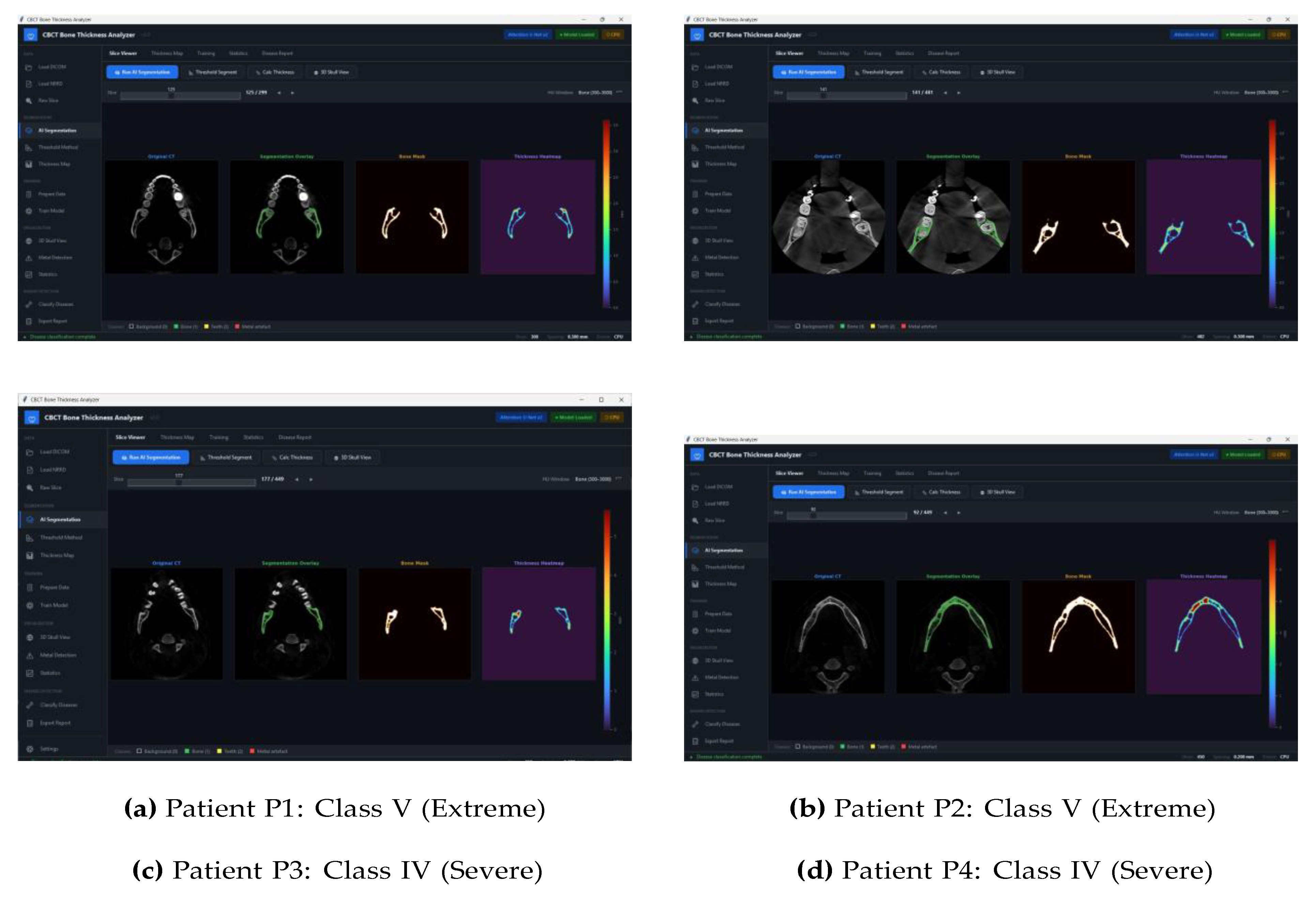
Table 1.
Segmentation performance on 443 ToothFairy patients (HU pseudo-ground truth).
| Metric | Value | Interpretation |
|---|---|---|
| Bone Dice (mean ± std) | 0.884 ± 0.020 | Strong; all cases above 0.7 |
| Bone Dice range | 0.798–0.938 | Consistent across scanner types |
| Bone Dice ≥ 0.7 | 443/443 (100%) | No poor-performance cases |
| Teeth Dice (mean ± std) | 0.789 ± 0.087 | Variable; edentulous/metal cases |
| Bone IoU (mean ± std) | 0.793 ± 0.032 | Consistent with Dice |
| Hausdorff Distance (bone) | 11.10 ± 3.57 mm | Boundary-level precision |
Table 3.
Disease classification output for all 443 patients.
| Classification | Count | % | Clinical meaning |
|---|---|---|---|
| Ridge Class II | 2 | 0.5 | Approaching adequate bone |
| Ridge Class III | 115 | 26.0 | Narrow implants (3–4 mm) |
| Ridge Class IV | 321 | 72.5 | Augmentation required |
| Ridge Class V | 5 | 1.1 | Major reconstruction needed |
| Augmentation / reconstruction (IV+V) | 326 | 73.6 | Cannot proceed directly |
| Standard implants feasible (I+II) | 2 | 0.5 | Subject to site assessment |
| MRONJ Low Risk | 443 | 100 | Normal density throughout |
| MRONJ Monitor | 0 | 0 | No flags triggered |
Disclaimer/Publisher’s Note: The statements, opinions and data contained in all publications are solely those of the individual author(s) and contributor(s) and not of MDPI and/or the editor(s). MDPI and/or the editor(s) disclaim responsibility for any injury to people or property resulting from any ideas, methods, instructions or products referred to in the content. |
© 2026 by the authors. Licensee MDPI, Basel, Switzerland. This article is an open access article distributed under the terms and conditions of the Creative Commons Attribution (CC BY) license (http://creativecommons.org/licenses/by/4.0/).
Copyright: This open access article is published under a Creative Commons CC BY 4.0 license, which permit the free download, distribution, and reuse, provided that the author and preprint are cited in any reuse.