

Submitted:
09 May 2026
Posted:
13 May 2026
You are already at the latest version
Abstract
Early 2026 has witnessed significant volatility in the oil market, and an energy crisis is expected in the coming months. Large-scale LLM inference continues to consume substantial power in data centers and improving inference efficiency is therefore increasingly important for energy sustainability of AI economy. Semi-structured N:M sparsity, most notably 2:4 (50%) and potentially 1:4 (75%), offers a hardware-friendly path to lower compute and energy, and has been supported in modern GPU designs. Yet existing training methods for 2:4 sparsity (e.g., STE-based approaches) often incur large accuracy drops relative to dense baselines, and practical support for 1:4 remains limited in current software stacks. As a result, attention has shifted toward quantization and mixture-of-experts, leaving high-sparsity N:M pre-training underexplored. Here we introduce a paradigm shift: we treat neural networks as complex systems whose sparse connectivity can be trained using network-science principles formalized by Cannistraci–Hebb sparse-to-sparse training (CHT), coupled with a tailored optimizer. We propose CHTsNM, a sparse-to-sparse training framework centered on Topology-Aware Newton–Schulz (TANS) optimization. TANS makes Newton–Schulz-style matrix updates compatible with dynamically changing semi-structured sparse topologies via active-mask projection, active-support RMS matching, and refresh-aware ramping after topology updates. CHTsNM further incorporates two lightweight mechanisms: Contextually Modulated LoRA (CoMoLoRA) for input-adaptive low-rank residual compensation, and Motif Pattern Revisitation (MPR) to improve exploration of legal row-wise N:M patterns. Across 4 LLaMA pre-training benchmarks, CHTsNM with 2:4 sparsity achieves performance close to dense baselines on most tasks and yields sparse-over-dense gains on 8 tasks. 1:4 sparsity approaches dense performance, though does not yet consistently surpass it. For hardware evaluation, we report measured speedups for native 2:4 execution on current NVIDIA GPUs, and provide a clearly labeled CSR sparse-GEMM surrogate analysis to estimate the acceleration potential of 1:4. Overall, although not implement on hardware yet, our results identify 1:4 sparse pre-training as a promising direction and establish TANS sparse-to-sparse optimization as a practical step toward future high-sparsity N:M accelerators.
Keywords:
semi-structured sparsity
; dynamic sparse training
; contextual modulation branch
; low rank branch
; newton–schulz
; optimizer
1. Introduction
Semi-structured sparsity has become a central hardware-oriented sparsity format for neural network acceleration [1]. Its most established instance is 2:4 sparsity, where two nonzero weights are retained in every group of four [2]; this format is natively supported by NVIDIA sparse Tensor Cores and has become the de facto reference point for semi-structured sparse training and pruning. A natural next algorithmic question is whether the same local N:M principle can be pushed to a more restrictive regime, such as 1:4 sparsity, where only one weight remains active in every group of four [3,4]. This setting is attractive because it preserves the group-of-four structure familiar from 2:4 sparsity while increasing the sparsity ratio to 75%. The main difficulty, however, is no longer only how to exploit a sparse pattern at inference time, but whether pre-training can preserve model quality under such an extreme legal constraint.
Although our title is hardware motivated, the technical claim of this paper is algorithmic. Current NVIDIA GPUs provide native sparse Tensor Core support for 2:4 execution, but not for native 1:4 execution. We therefore do not claim measured native 1:4 speedup on current NVIDIA hardware. Throughout the paper, “1:4 NVIDIA sparsity” refers to a hardware-forward N:M target that keeps the local group-of-four structure of the existing NVIDIA semi-structured sparsity interface, rather than to an already deployed NVIDIA execution mode. We want to clarify that many efficient-AI techniques first emerge as algorithmic evidence, and then hardware manufacturers provide support for them, such as 8-bit Training [5,6,7,8]. Our primary contribution is to study whether sparse pre-training algorithms can make this more aggressive 1:4 target viable in model quality. For hardware evaluation, we report measured speedups only for native 2:4 execution on NVIDIA hardware, and we separately provide a clearly labeled CSR sparse-GEMM surrogate as a projection for potential future 1:4 acceleration.
In this work, we show that moving from 2:4 to 1:4 sparsity is not a simple increase in sparsity ratio, but a regime shift in sparse pre-training. The 1:4 constraint changes the optimization problem in three coupled ways. First, proxy-gradient dense-to-sparse methods [3,9] become increasingly mismatched with the actually executed sparse model, because most weights in each local group are inactive in the forward pass while still receiving surrogate gradients. Second, low-rank residual branches [10] become more valuable, because the sparse backbone loses most local degrees of freedom and therefore needs an explicit compensation path for missing function directions. Third, matrix-geometry optimizers such as Muon-style [11] Newton–Schulz updates are promising but cannot be directly transplanted into dynamic sparse training, because the active support changes after each topology refresh. Appendix A provides the supporting sparsity-regime studies.
The first regime-shift signal concerns topology learning. Existing semi-structured sparse training methods such as STE-based [12] training typically maintain dense latent weights and use Straight-Through Estimator surrogate gradients to update weights that are masked out in the forward computation. This mismatch is moderate in 2:4 sparsity, where half of the weights in each local group remain active, but it is amplified in 1:4 sparsity, where three quarters of the weights are inactive during the forward pass [13]. This motivates true sparse-to-sparse training: only active weights are optimized, and the sparse topology evolves through legal remove-regrow operations. As shown in Table A1, the gap between proxy-gradient training and sparse-to-sparse topology learning widens sharply as the legal support becomes more restrictive, supporting the view that 1:4 requires a different training paradigm.
The second signal concerns residual capacity. In standard dense-model adaptation, LoRA is usually introduced as a lightweight task-adaptation module on top of an already expressive pretrained model [14]. In semi-structured sparse pre-training, its role is different: the auxiliary low-rank branch acts as a train-from-scratch residual compensation path for function directions suppressed by the sparse backbone. Table A2 shows that the gain from a 1M-param LoRA branch grows as the sparsity pattern becomes more restrictive. This does not by itself make low-rank compensation the main contribution of our method, but it motivates including a small residual branch when studying the extreme 1:4 regime.
The third and most important signal concerns optimization. Recent matrix-geometry optimizers [15] can substantially improve dense neural network training by shaping updates at the matrix level rather than treating coordinates independently [16]. Our sparsity-level optimizer sweep in Table A3 shows that such geometry is also useful for sparse pre-training. However, dynamic N:M sparse training introduces a topology mismatch that dense optimizers do not face: after each refresh, removed weights leave the executed model, newly activated weights enter with little optimizer history, and a dense matrix update may place mass on inactive coordinates. This identifies the central technical bottleneck of 1:4 sparse-to-sparse pre-training: matrix geometry must be made compatible with a changing legal sparse support.
Motivated by this diagnosis, we propose CHTsNM, a true sparse-to-sparse training framework centered on Topology-Aware Newton–Schulz optimization (TANS). TANS is the main technical contribution of this work. It adapts Newton–Schulz-style matrix updates to dynamic semi-structured sparse topology through three design choices: active-mask projection, which prevents the optimizer from becoming a hidden dense optimizer; active-support RMS matching, which preserves the trusted magnitude of the sparse preconditioned base update; and refresh-aware ramping, which gradually restores matrix geometry after topology changes. In this sense, TANS is not a direct application of Muon or a generic dense matrix optimizer to sparse weights, but a topology-aware interface between sparse preconditioning and matrix-level update geometry.
CHTsNM includes two lightweight supporting mechanisms around TANS. First, Contextually Modulated LoRA (CoMoLoRA) treats the auxiliary branch as an input-adaptive residual compensator for missing sparse-backbone directions. It starts from standard LoRA and modulates the LoRA rank space with input context, so the residual branch can emphasize or suppress compensation directions for different tokens. Second, Motif Pattern Revisitation (MPR) extends CHTs24-style sparse-to-sparse topology learning from block-wise motifs to row-wise N:M masks and discourages ineffective same-pattern revisits during row-wise refresh. We emphasize that CoMoLoRA and MPR are not positioned as equally central innovations to TANS. They are supporting mechanisms designed to test two consequences of the 1:4 regime shift: the increased value of residual compensation and the need for effective row-wise legal-pattern exploration.
We evaluate CHTsNM on LLaMA [17] pre-training benchmarks, focusing on 1:4 sparsity with additional 2:4 comparisons to characterize the sparsity-regime transition. We compare CHTsNM against STE [18], SR-STE [3], CAST [19], and CHTs24 [13] as the main method-level baselines. Each baseline is evaluated under its intended sparse-training rule, while CHTsNM uses TANS because topology-aware optimization is the proposed method rather than an external tuning advantage. To make this optimizer contribution explicit, we also provide an optimizer-controlled diagnostic in which the CHTs24 topology engine is fixed and only the update rule is changed. This separates the question of whether CHTsNM outperforms prior sparse-training recipes from the question of which optimizer design choices account for the gain.
The empirical results support the TANS-centered interpretation. CHTsNM substantially outperforms STE, SR-STE, CAST, and CHTs24 under matched sparsity settings, and its no-branch variant already improves strongly over prior sparse baselines, showing that the gain is not merely due to auxiliary parameters. Ablations show that TANS contributes the dominant improvement, while CoMoLoRA and MPR provide smaller but complementary gains in the regimes where they are designed to help. Together, these results suggest that 1:4 sparse pre-training can be very close to dense-level quality when dynamic sparse topology is paired with topology-aware matrix optimization, and when residual compensation and row-wise pattern exploration are added as targeted supporting mechanisms.
Our contributions are summarized as follows:
- We provide a systematic study of the transition from 2:4 to 1:4 semi-structured sparse pre-training, identifying 1:4 sparsity as a regime shift rather than a linear increase in sparsity ratio. We also explicitly separate this algorithmic study from any claim of currently available native 1:4 execution on NVIDIA GPUs.
- We propose Topology-Aware Newton–Schulz optimization (TANS), a refresh-aware matrix optimizer for dynamic N:M sparse-to-sparse training. TANS makes matrix-geometry updates compatible with changing sparse supports through active-mask projection, active-support scale matching, and refresh-aware ramping.
- We instantiate TANS inside CHTsNM, a practical sparse-to-sparse training framework for extreme N:M sparsity. CHTsNM includes two supporting mechanisms: CoMoLoRA for input-adaptive low-rank residual compensation, and MPR for row-wise legal-pattern exploration.
- We provide method-level, component-level, and optimizer-controlled experiments showing that TANS is the dominant source of improvement, while CoMoLoRA and MPR provide complementary gains. We further separate measured native 2:4 speedups from a clearly labeled CSR surrogate analysis for potential future 1:4 acceleration.
2. Related Work
N:M semi-structured sparsity and hardware scope.
N:M semi-structured sparsity restricts each group of M weights to contain at most N nonzeros [1,2,3]. Its most established hardware instance is 2:4 sparsity, which is supported by NVIDIA sparse Tensor Cores. In this work, 1:4 sparsity is used as a hardware-forward algorithmic target: it preserves the group-of-four structure while increasing sparsity to 75%. We do not assume native 1:4 execution on current NVIDIA GPUs; instead, we study whether sparse pre-training algorithms can make this more restrictive N:M target viable in model quality. We evaluate both row-wise and block-wise layouts, since row-wise masks naturally align with forward sparse multiplication, whereas block-wise or transposable N:M masks better preserve sparse structure across forward and backward computations [18,20].
Dense-to-sparse versus sparse-to-sparse N:M training.
Most N:M sparse training methods were developed around the 2:4 regime. STE-based training, SR-STE [3], S-STE [9], and continuous projection methods such as CAST [19] maintain dense or dense-latent parameters and use surrogate gradients or gradual projection to obtain legal sparse weights. This dense-to-sparse design becomes increasingly mismatched with the executed sparse model as the legal support becomes more restrictive. True sparse-to-sparse training instead optimizes only active weights and evolves topology through legal remove-regrow transitions. CHTs24 [13] is a representative sparse-to-sparse method for semi-structured topology learning. CHTsNM builds on this principle, extends it to the 1:4 regime and row-wise N:M masks, and introduces topology-aware matrix optimization as the central missing component.
Sparse residual compensation.
Low-rank branches are an effective way to recover capacity lost by sparse backbones. CHTsL [21] studies CHT-style sparse backbones with LoRA-like branches, while SLTrain [22] represents a broader sparse-plus-low-rank pre-training paradigm. For semi-structured sparsity, HASSLE-Free [23], SLOPE [24], and ARMOR [25] show that low-rank or factorized auxiliary capacity can improve the quality–efficiency trade-off of sparse models. Our CoMoLoRA component follows this residual-compensation view, but adds input-conditioned rank-space modulation inspired by contextual modulation methods such as Transponder [26]. We position CoMoLoRA as a lightweight supporting mechanism for 1:4 sparse pre-training, rather than as the main source of improvement.
Matrix-geometry optimization under changing sparse support.
Most semi-structured sparse training methods rely on Adam-style coordinate-wise optimizers; for example, CAST [19] proposes AdamS. In parallel, matrix-geometry optimizers updates [11] improve dense training by shaping updates at the matrix level. These optimizers, however, assume a stable dense parameterization. Dynamic N:M sparse training changes the active support after each topology refresh, so newly activated weights have limited optimizer history and unconstrained matrix updates may place mass on inactive coordinates. TANS bridges this gap by using Newton–Schulz geometry only as a masked, scale-calibrated, and refresh-aware residual correction on the active support.
A more detailed discussion is provided in Appendix B.
3. Method
3.1. Overview of CHTsNM
CHTsNM is designed for true sparse-to-sparse pre-training under legal semi-structured masks. For each target linear layer, we write the executed sparse weight as . Unlike dense-to-sparse methods based on STE-style surrogate gradients, inactive weights are not used in the forward pass and are not updated. The mask evolves only through legal topology refreshes.
The framework has three components, ordered by their role in the training pipeline. First, Topology-Aware Newton–Schulz (TANS) is the main optimization component: it makes matrix-geometry updates compatible with changing sparse supports. Second, Contextually Modulated LoRA (CoMoLoRA) adds a small input-adaptive residual branch to compensate for function directions removed by the sparse backbone. Third, Motif Pattern Revisitation (MPR) improves the effectiveness of row-wise topology refreshes by discouraging ineffective same-pattern revisits. In a target linear layer with CoMoLoRA enabled, the output is
where TANS optimizes the sparse backbone , Adam optimizes the dense low-rank branch, and MPR modifies only the row-wise mask-refresh candidate set.
3.2. TANS: Topology-Aware Newton–Schulz Optimization
Modern matrix optimizers, such as Muon-style Newton–Schulz updates, suggest that matrix-level update geometry can improve neural network training. However, dynamic semi-structured sparse training introduces a topology mismatch that does not exist in dense optimization. In CHTsNM, the sparse backbone is optimized under a changing active support: after each topology refresh, removed weights leave the executed model, while newly activated weights enter the forward computation with little optimizer history. Therefore, a dense matrix-geometry update can be stale with the current legal sparse topology. TANS addresses this issue by using Newton–Schulz geometry as a topology-aware residual correction on top of a masked preconditioned base update.
For a sparse weight matrix , TANS first restricts optimization to the active support by using the masked gradient . To stabilize optimization under the highly constrained 1:4 backbone, we compute a preconditioned gradient and a momentum-smoothed base direction:
This base update is not intended as a new optimizer family by itself. Instead, it provides a sparse-compatible direction whose magnitude is reliable on the actually executed support.
TANS then computes a Newton–Schulz matrix-geometry direction from the base update. We normalize and apply polynomial Newton–Schulz iterations:
The resulting matrix gives a matrix-shaped correction direction. For rectangular matrices, we transpose the update when needed so that the iteration is applied on the lower-dimensional side, and transpose it back afterward. The coefficient values are listed in Appendix C.
The topology-aware part of TANS consists of two legality and stability steps. First, since Newton–Schulz is a matrix operation, its output may contain nonzero values on inactive coordinates. TANS projects the correction back to the current active support , which prevents the optimizer from becoming a hidden dense optimizer and preserves true sparse training. Second, TANS matches the correction scale using only active entries:
Here denotes the RMS computed over the active support of . Active-support RMS matching lets the Newton–Schulz transform control update geometry while retaining the trusted magnitude of the sparse preconditioned base update.
Finally, TANS makes the geometry correction aware of topology age. Let be the number of optimizer steps since the last topology refresh of the current sparse matrix. We use a refresh ramp and form the final sparse-backbone update direction as .
Immediately after a topology refresh, TANS stays close to the stable preconditioned base optimizer. As the active support becomes older and more reliable, the Newton–Schulz geometry correction is gradually restored. This refresh-age modulation is the key distinction between TANS and directly applying a dense Muon-style optimizer to a dynamically sparse backbone.
The parameter update uses AdamW-style decoupled weight decay and a fan-ratio learning-rate scale . TANS first applies multiplicative weight decay and then takes the sparse update step:
We apply TANS only to the semi-structured sparse backbone. CoMoLoRA parameters are optimized with Adam because the low-rank branch has a stable dense parameterization and does not undergo topology refresh. Thus, TANS is designed not as a generic optimizer for all parameters, but as a topology-aware interface between sparse preconditioning and matrix-geometry optimization under changing 1:4-active supports.
3.3. CoMoLoRA: Contextual Low-Rank Residual Compensation
Under 1:4 sparsity, the sparse backbone removes most local degrees of freedom, so a low-rank branch acts as a train-from-scratch residual compensation path rather than a standard adaptation module. CoMoLoRA makes this compensation input-adaptive by modulating the LoRA rank space:
The last layer of G is initialized to zero, so at initialization and CoMoLoRA starts exactly as standard LoRA. During training, it gradually learns input-dependent residual compensation for the sparse backbone. Appendix D shows the details and motivation of CoMoLoRA.
3.4. From Block-Wise CHTs24 to Row-Wise CHTsNM via Motif Pattern Revisitation
CHTs24[13] does not define a row-wise topology operator. CHTsNM supports row-wise semi-structured masks by partitioning each row into local groups of four weights and constraining each group to choose a legal row-wise pattern . This extension preserves true sparse-to-sparse training: inactive weights are not used in the forward pass and are not updated. For a row group g with regrowth score , the standard row-wise projection selects the highest-scoring legal pattern from . However, in row-wise 1:4 there are only four legal patterns, so a refresh step may repeatedly select the previous pattern and produce little effective topology change. MPR addresses this issue by suppressing same-pattern revisitation with probability , and full details are provided in Appendix E.
4. Experiments
4.1. Main Results: Narrowing the 1:4 Sparse–Dense Gap
Table 1 compares CHTsNM with STE, SR-STE, CAST, and CHTs24 under matched sparsity settings. Under 1:4 sparsity, CHTsNM with a 1% auxiliary branch reduces the PPL of the strongest CHTs24 baseline by on LLaMA-60M and on LLaMA-130M, averaged over row-wise and block-wise layouts. The resulting 1:4 models are only and above the dense references on LLaMA-60M and LLaMA-130M, respectively. At the 2:4 sparsity, CHTsNM still outperforms dense on the LLaMA-350M model.
The no-branch variant of CHTsNM already outperforms all sparse baselines across both 1:4 and 2:4 regimes, indicating that the gain is not merely due to adding auxiliary parameters. The 1% CoMoLoRA branch further improves the 1:4 results, where the sparse backbone has fewer local degrees of freedom. Appendix F visualizes these results, and Appendix G reports consistent zero-shot improvements on WikiText [27], LAMBADA [28], SciQ [29], and ARC-Easy [30].
These results support the central empirical claim: 1:4 sparsity can approach dense-quality pre-training when sparse topology learning, residual compensation, and topology-aware optimization are redesigned jointly. Section 3.2 further studies the optimization component, and Appendix H provides baseline and training details.
4.2. Ablation: TANS Is the Primary Driver
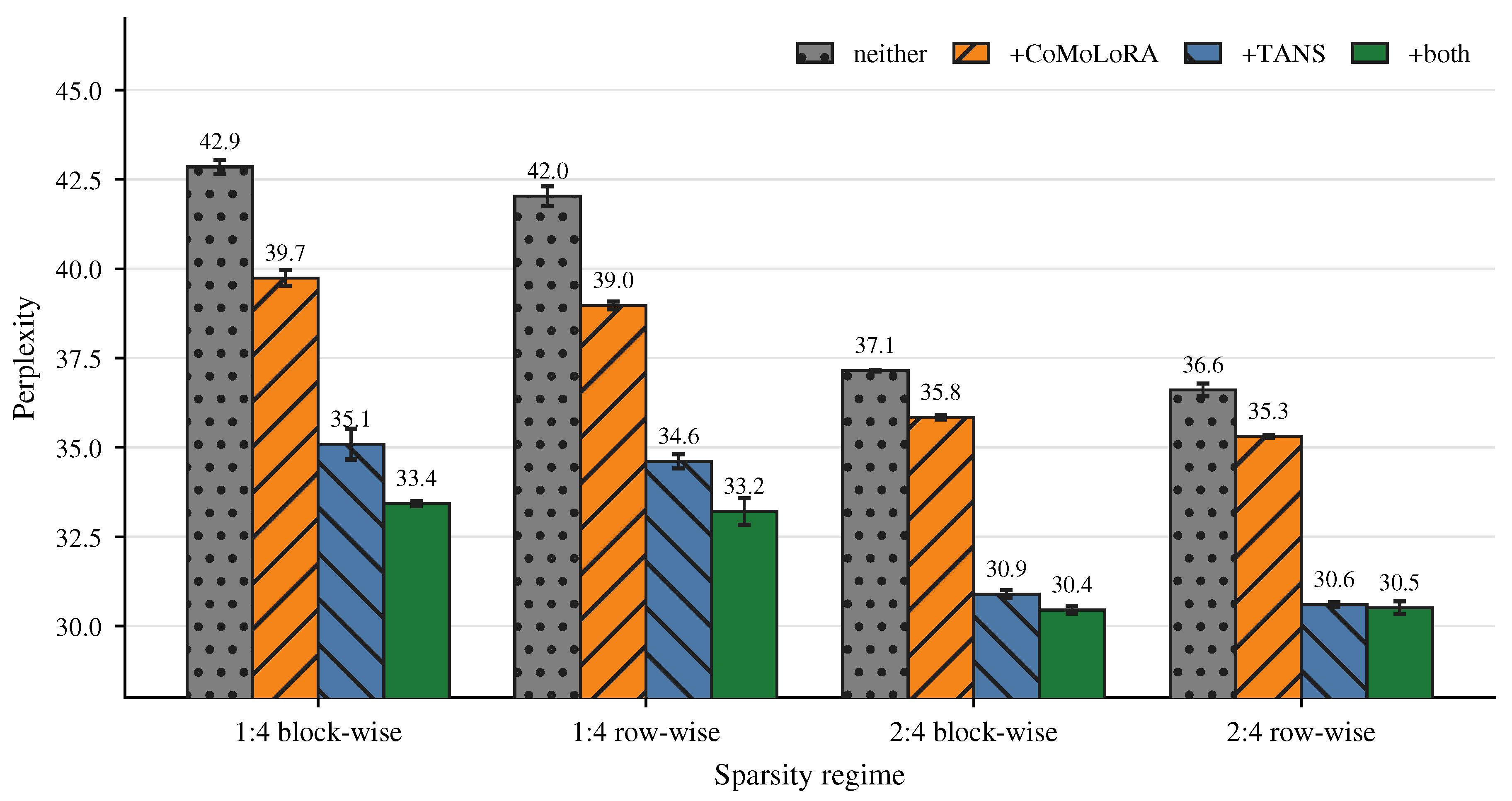
Table 2 isolates the two main components of CHTsNM across sparsity regimes and mask layouts. The largest improvement comes from TANS. Averaged over row-wise and block-wise results, adding TANS reduces PPL by under 1:4 sparsity and under 2:4 sparsity. CoMoLoRA provides a smaller but complementary gain: by itself, it reduces PPL by under 1:4 and under 2:4. When combined with TANS, CoMoLoRA gives an additional reduction under 1:4, compared with under 2:4. This supports two conclusions: topology-aware optimization is the main bottleneck, and residual low-rank compensation becomes more valuable as the sparsity pattern becomes more restrictive. Appendix F visualizes this ablation.
4.3. Why Dense Matrix Geometry Needs Topology Awareness
We next analyze whether matrix-geometry optimization can be directly transferred to dynamic 1:4 sparse pre-training. Table 3 compares increasingly sparse-compatible update rules under the same CHTs24 backbone. Geometry alone is not sufficient: the geometry-only update performs worse than AdamW. In contrast, a sparse preconditioned base update gives a large gain, and Newton–Schulz geometry becomes beneficial only when used as a residual correction on top of this sparse base. TANS further improves the correction by matching its active-support RMS scale and ramping it after topology refreshes, yielding the best operating point.
Appendix I.1 shows that RMS matching is not a brittle one-point trick; rather, it becomes essential for stability when is high. Removing RMS matching degrades PPL to , whereas either RMS-matching variant recovers it to . Appendix I.2 shows that refresh ramping is consistently useful under dynamic sparse topology. Moreover, explicit optimizer-state repair after refresh is complementary to ramping rather than a replacement for it, as detailed in Appendix I.3.
Overall, Appendix I shows that the gain does not come from a single fragile coefficient choice, but from a coherent response to dynamic sparse topology: keeping matrix-geometry updates numerically aligned, softening the post-refresh transition, and repairing optimizer history where the support actually changes.
This mechanism ablation separates the sparse base update, matrix-geometry correction, and scale control under one sparse setting. The optimizer benchmark in Table A9 in Appendix J evaluates whether TANS can be replaced by existing optimizers; TANS achieves the lowest final PPL for dense, CHTs 2:4, and CHTs 1:4 training, with the largest gap at 1:4 compared with AdamW and Muon.
4.4. Auxiliary Branch and Contextually Modulated LoRA
Design space.
Under 1:4 sparsity, the sparse backbone loses many local degrees of freedom, so an auxiliary branch should act as residual compensation rather than only as a standard adaptation module. We compare whether the branch should add new low-rank directions [24], align with the sparse backbone [21], or multiplicatively modulate sparse features [26].
Let be the sparse-backbone output. We write the auxiliary-branch family as
where controls product modulation on the sparse output, controls rank-space modulation inside the low-rank branch, and indicates whether an additive residual branch is used. This form covers additive low-rank compensation, alignment-regularized compensation, product-only contextual gating, and CoMoLoRA. We denote these variants as Add, Add+Align, Prod-Gate, and CoMo, respectively; full formulas are provided in Appendix K.
Results.
Table 4 shows that Add+Align is strongest at the 1% budget, where the rank-space gate has limited modulation capacity. From 2% to 5%, CoMoLoRA consistently obtains the best PPL, indicating that additive residual compensation and contextual rank-space modulation are complementary. The small gap between Add and Add+Align suggests that, under 1:4 sparsity, the auxiliary branch should primarily recover residual directions missing from the sparse backbone rather than directly mimic the sparse output.
4.5. Motif Pattern Revisitation
Finally, we evaluate MPR as a row-wise topology-refresh refinement. On row-wise 1:4, all tested MPR values reduce PPL by more than 1% relative to disabling MPR, with the best setting reducing PPL by . On row-wise 2:4, the best tested setting gives a smaller PPL reduction.
This difference is expected: under row-wise 1:4, changing the motif relocates the only active position in each group, so overly aggressive forcing can be disruptive; under row-wise 2:4, a motif change can preserve one active position and tolerate stronger revisit suppression. MPR is also not equivalent to increasing the DST refresh ratio : changing controls how many groups are refreshed, whereas MPR controls whether a selected group actually changes its legal pattern. Detailed MPR statistics and controls are provided in Appendix L.
5. Inference Speedup
Since the ablation shows that the LoRA branch is less important under 2:4 sparsity, we isolate the sparse backbone and measure its inference acceleration on current NVIDIA hardware. Table 5 reports the speedup of trained CHTsNM sparse-backbone checkpoints. The speedup increases with model scale and reaches up to on LLaMA-1B.
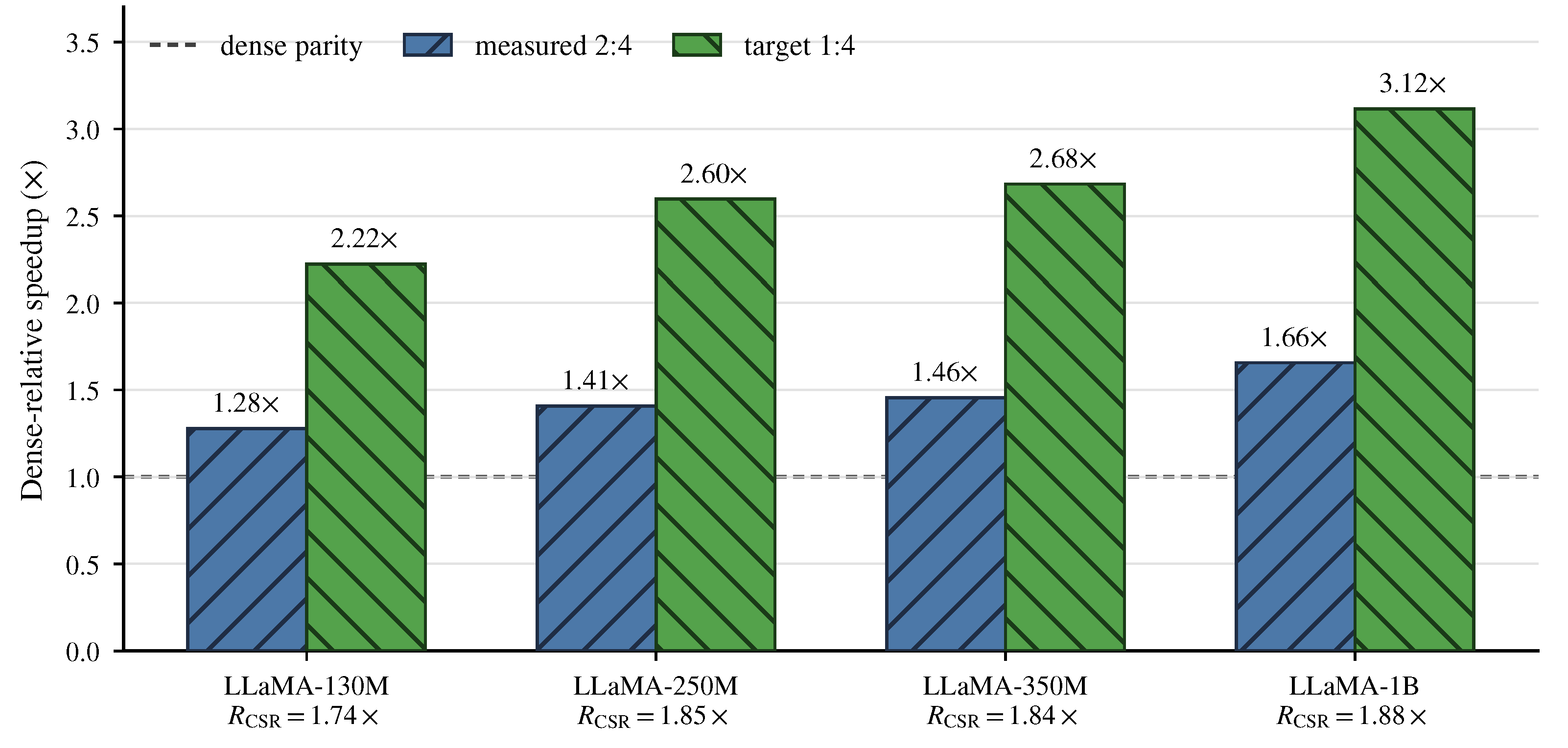
Current NVIDIA hardware does not support 1:4 execution. We therefore analyze 1:4 acceleration with a matched CSR sparse-GEMM surrogate. The CSR analysis gives an average relative runtime improvement from 2:4 to 1:4, which maps the best measured 2:4 result to a first-order target speedup of approximately . Full throughput tables, hardware details, and the extrapolation protocol are provided in Appendix M.
6. Conclusion
We studied 1:4 semi-structured sparse pre-training as a more restrictive regime beyond standard 2:4 sparsity. Our results suggest that this transition changes the training problem: proxy-gradient dense-to-sparse methods become increasingly mismatched with the executed sparse model, low-rank residual capacity becomes more important, and matrix-level optimizers must respect changing sparse supports. Motivated by these observations, CHTsNM keeps the executed backbone sparse-to-sparse and jointly adapts topology refresh, residual compensation, and optimization for the 1:4 regime.
Empirically, TANS is the main contributor, making Newton–Schulz-style matrix geometry compatible with dynamic sparse topology through masked updates, active-support scale matching, and refresh-aware ramping. CoMoLoRA further improves input-adaptive residual compensation, especially under 1:4 sparsity, while MPR improves row-wise legal-pattern exploration. Together, these components substantially narrow the PPL gap between 1:4 models and dense references across LLaMA pre-training experiments. Since current hardware only provides native 2:4 sparse Tensor Core support, our 1:4 results should be interpreted as an algorithmic step toward future high-sparsity N:M hardware rather than a measured 1:4 deployment claim. We list the limitation of our research in Appendix N
Appendix A. From 2:4 to 1:4: A Paradigm Shift Rather than a Linear Sparsity Increase
We summarize three targeted regime-shift studies. Together, they show that the transition from 2:4 to 1:4 is not just a higher sparsity ratio: it changes which training mechanisms work best. Across topology learning, optimizer choice, and auxiliary residual compensation, the 1:4 regime amplifies the weaknesses of dense-oriented baselines and increases the value of sparse-aware or residual-aware mechanisms. All numbers below come from the current 100M-token evaluation snapshot of the dedicated regime-shift runs with LLaMA-60M and block-wise sparsity.
Appendix A.1. Sparse-to-Sparse Training Matters Much More at 1:4
Our first study compares a sparse-to-sparse backbone (CHTs24) against the dense-to-sparse baseline (STE). At light sparsity the difference is visible but modest, while at 1:4 it becomes large. The key point is not only that CHTs24 is better, but that the gap widens sharply as the feasible support shrinks.

Table A1.
Sparse training regime shift from STE to CHTs24. The PPL gap widens strongly as we move from 3:4 to 2:4 and especially to 1:4 sparsity.
Table A1.
Sparse training regime shift from STE to CHTs24. The PPL gap widens strongly as we move from 3:4 to 2:4 and especially to 1:4 sparsity.
| Regime | Sparsity | CHTs24 PPL | STE PPL | STE − CHTs24 |
|---|---|---|---|---|
| block-wise 3:4 | 25% | 32.41 | 34.02 | 1.60 |
| block-wise 2:4 | 50% | 34.46 | 38.45 | 3.99 |
| block-wise 1:4 | 75% | 42.85 | 53.91 | 11.06 |
The most relevant transition for the main paper is the jump from 2:4 to 1:4: the PPL gap increases from to . This supports the view that the 1:4 setting requires a sparse-to-sparse training method rather than a purely straight-through sparse proxy.
Appendix A.2. The Value of a LoRA Residual Branch Grows with Sparsity
Our second study examines a fixed 1M-param LoRA residual branch on top of static sparse backbones. Here the regime-shift pattern is especially clear: the denser settings already benefit slightly from LoRA, but the gain grows rapidly as sparsity becomes more severe. This is consistent with the interpretation that, under 1:4 sparsity, the low-rank branch is increasingly acting as a residual compensation path for missing local degrees of freedom.
Table A2.
Value of a fixed small LoRA branch as sparsity increases. The benefit grows from a minor dense improvement to a much larger gain at 1:4.
Table A2.
Value of a fixed small LoRA branch as sparsity increases. The benefit grows from a minor dense improvement to a much larger gain at 1:4.
| Regime | Sparsity | Anchor PPL | +LoRA PPL | PPL Gain | Gain vs Dense Gain |
|---|---|---|---|---|---|
| Dense | 0% | 32.70 | 32.38 | 0.32 | |
| Block-Wise 3:4 | 25% | 34.53 | 33.70 | 0.84 | |
| Block-Wise 2:4 | 50% | 37.19 | 35.66 | 1.54 | |
| Block-Wise 1:4 | 75% | 42.81 | 39.19 | 3.62 |
The most important comparison again is 2:4 versus 1:4. The LoRA branch improves PPL by points at 2:4, but by points at 1:4. This suggests that the 1:4 regime increasingly rewards methods that restore missing capacity through an explicit residual path rather than relying only on the sparse backbone.
Appendix A.3. Dense-Oriented Optimizer Geometry Does Not Remove the 1:4 Transition
Our third study compares Muon against an AdamW anchor on the same static sparse backbones. In absolute sparse PPL, Muon remains better than AdamW at all three sparsity levels. However, relative to each optimizer’s own dense baseline, Muon still suffers large degradation as sparsity tightens. This makes the optimizer picture more nuanced than the topology picture: better dense geometry helps, but it does not neutralize the 1:4 transition.
Table A3.
Muon versus AdamW across sparsity regimes. “dense” denotes the PPL increase relative to the dense model trained by the same optimizer. Muon keeps a better absolute sparse PPL, but both optimizers degrade substantially by 1:4.
Table A3.
Muon versus AdamW across sparsity regimes. “dense” denotes the PPL increase relative to the dense model trained by the same optimizer. Muon keeps a better absolute sparse PPL, but both optimizers degrade substantially by 1:4.
| Regime | Sparsity | Muon PPL | AdamW PPL | Muon | AdamW |
|---|---|---|---|---|---|
| Block-Wise 3:4 | 25% | 31.55 | 34.33 | 1.73 | 1.81 |
| Block-Wise 2:4 | 50% | 34.18 | 37.19 | 4.36 | 4.68 |
| Block-Wise 1:4 | 75% | 39.34 | 42.74 | 9.52 | 10.22 |
The takeaway is that the transition from 2:4 to 1:4 is not solved by optimizer choice alone. Even when Muon remains the stronger absolute optimizer, the sparse penalty still grows sharply at 1:4, indicating that the core difficulty is structural rather than purely geometric.
Summary. Taken together, these three studies motivate our broader claim that the jump from 2:4 to 1:4 is a genuine training-regime transition. At 1:4, sparse-to-sparse training method becomes much more important, optimizer improvements alone do not remove the sparse penalty, and dense residual compensation becomes substantially more valuable.
Appendix B. Extended Related Work
Semi-structured sparsity. N:M semi-structured sparsity is a hardware-oriented sparsity format that constrains local groups of weights rather than pruning arbitrary individual weights. The best-known instance is 2:4 sparsity, where two weights remain active in every group of four. This format is supported by NVIDIA sparse Tensor Cores and has become the de facto reference point for semi-structured sparse training and pruning [1,2]. Compared with unstructured sparsity, N:M sparsity is easier to map to regular hardware kernels; compared with coarse structured sparsity, it preserves more local modeling flexibility.
The hardware status of 1:4 sparsity is different. Current NVIDIA GPUs do not provide native 1:4 sparse Tensor Core execution. Therefore, our use of 1:4 should be understood as an algorithmic and hardware-forward target rather than a claim of currently deployed NVIDIA acceleration. This distinction is important: our main paper evaluates whether high-quality pre-training is possible under such a restrictive N:M constraint, while measured hardware acceleration is reported only for currently supported 2:4 execution.
The layout of the N:M constraint also matters. Row-wise N:M sparsity is simple and naturally matches the forward multiplication of linear layers. However, the transposed operands used in backpropagation generally do not preserve the same row-aligned sparsity. Block-wise, or transposable, N:M sparsity imposes compatible constraints along both dimensions, which can better preserve sparse structure in both forward and backward passes [18,20]. For this reason, we evaluate both row-wise and block-wise layouts in the main experiments.
Semi-structured sparse training. Existing N:M sparse training methods mainly focus on the 2:4 setting. STE-based methods maintain dense or dense-latent weights and use a Straight-Through Estimator to propagate gradients through the sparse projection. SR-STE [3] and S-STE [9] improve this training paradigm with sparsity-aware surrogate-gradient designs. CAST [19] follows a continuous-projection view and gradually projects dense weights into legal sparse patterns.
These dense-to-sparse methods are natural for 2:4 sparsity, where half of the local weights remain active. However, in the 1:4 regime, only one weight in each group of four participates in the executed forward computation. The mismatch between dense-latent optimization and the actually executed sparse model is therefore amplified. This motivates true sparse-to-sparse training, where inactive weights are not optimized as hidden dense parameters and topology changes are performed through legal remove-regrow transitions.
CHTs24 [13] is closely related to our work because it represents a true sparse-to-sparse approach to semi-structured topology learning. However, CHTs24 is primarily formulated around block-wise topology updates and does not provide the full optimizer interface needed for dynamic 1:4 sparse pre-training. CHTsNM extends this sparse-to-sparse principle to the more restrictive 1:4 regime, supports row-wise N:M masks, and introduces TANS to make matrix-level optimization compatible with changing sparse supports.
Sparse-plus-low-rank residual compensation. Sparse models often lose expressive capacity because the sparse backbone cannot represent all directions available to a dense model. Low-rank branches provide a parameter-efficient way to recover part of this missing capacity. CHTsL [21] studies LoRA-like branches with CHT-style sparse backbones, while SLTrain [22] represents a broader sparse-plus-low-rank pre-training framework. HASSLE-Free [23] decomposes pretrained weights into sparse and low-rank components, and SLOPE [24] shows that lazy low-rank adapters can improve 2:4 sparse pre-training. ARMOR [25] further suggests that auxiliary factorized transformations are useful for recovering the accuracy of highly constrained sparse cores.
Our use of CoMoLoRA follows the same broad motivation, but the role of the low-rank branch is different from standard adaptation. In 1:4 sparse pre-training, the branch is trained from scratch together with the sparse backbone and acts as a residual path for function directions removed by the sparse mask. This is why we view CoMoLoRA as sparse residual compensation rather than ordinary downstream LoRA adaptation.
Contextual modulation. Contextual modulation methods, including Transponder [26], show that input-conditioned modulation can improve residual learning in LLMs. CoMoLoRA applies this idea inside the LoRA rank space. Instead of using one fixed global low-rank correction for all tokens, it learns an input-dependent modulation over rank directions. This is especially useful under restrictive sparse backbones, where the missing residual directions may vary across inputs.
We emphasize that CoMoLoRA is not positioned as the main contribution of this paper. Its role is to test the residual-compensation implication of the 1:4 regime shift. The main contribution is TANS, while CoMoLoRA provides a lightweight and complementary branch-level improvement.
Matrix-geometry optimization. Most sparse training methods use Adam-style coordinate-wise optimizers. These optimizers are robust and easy to combine with sparse masks, but they do not explicitly shape the update at the matrix level. Recent dense-training optimizers, including Muon-style Newton–Schulz methods [11], instead use matrix-level geometry to improve update directions. This has shown strong promise in dense neural network training.
However, dynamic sparse training introduces a problem that dense matrix optimizers do not face: the active support changes over time. After a topology refresh, some weights are removed from the executed model, while newly activated weights enter with little optimizer history. A dense matrix-geometry update can also assign update mass to inactive coordinates, which is inconsistent with true sparse-to-sparse training.
TANS addresses this gap by treating Newton–Schulz geometry as a residual correction on top of a sparse-compatible base update. It first projects the correction onto the active mask, then matches its RMS scale on the active support, and finally ramps the correction according to topology age after each refresh. In this way, TANS connects dense matrix-geometry optimization with dynamic N:M sparse training without turning the sparse backbone into a hidden dense optimizer.
Appendix C. The Coefficient Values of TANS
Inside TANS, the Newton–Schulz correction uses a fixed five-step polynomial update. Let X denote the normalized matrix fed into the iteration and let . Each step updates
The coefficient triples used in the current implementation are:
Table A4.
Fixed coefficient values used by the five-step Newton–Schulz correction.
| Step t | |||
|---|---|---|---|
| 1 | 4.0848 | 2.9270 | |
| 2 | 3.9505 | 2.6377 | |
| 3 | 3.7418 | 2.3037 | |
| 4 | 2.8769 | 1.2046 | |
| 5 | 2.8366 | 1.2012 |
These values are exactly the hard-coded coefficients in the current standalone TANS implementation. They are not tuned separately across the main paper experiments; instead, the experiments vary the higher-level TANS coefficients such as , the correction coverage fraction, RMS matching, and refresh ramping.
Appendix D. Motivation for CoMoLoRA
This appendix gives a more detailed motivation for CoMoLoRA, by which we mean a context-modulated low-rank compensation branch on top of a sparse backbone.
Appendix D.1. Sparse Pretraining Changes the Role of LoRA
In standard dense adaptation, LoRA is often interpreted as a lightweight task-adaptation module. Our setting is different. Under legal semi-structured sparsity such as , the executed backbone weight W has already lost most local degrees of freedom before training converges. As a result, the auxiliary low-rank branch is better understood as a train-from-scratch residual compensation path rather than as a conventional adapter.
Let denote the dense weight that would ideally be learned by a dense model under the same training budget, and let W denote the executed sparse weight. The missing output component is
Standard LoRA approximates this missing component by a fixed low-rank residual
This is already useful, because it supplies a dense compensation path that is not constrained by the sparse backbone mask. However, it is still a global low-rank compensator: all tokens share the same rank-space geometry and the same output directions.
Appendix D.2. A Least-Squares View of Residual Fitting
The residual-compensation interpretation can be made explicit through least squares. Suppose we have training activations and corresponding target residuals
Then standard LoRA can be viewed as solving the constrained regression problem
Equivalently, if we define the rank hidden state
then LoRA predicts
where is the k-th column of B. In this view, LoRA learns:
- a shared projection A that extracts rank-space coefficients, and
- a shared dictionary of output-space compensation directions.
This least-squares formulation also clarifies the limitation of standard LoRA in our sparse-pretraining regime. The best low-rank fit is forced to use a single global factorization to approximate a residual map whose structure may vary substantially across inputs. When the sparse backbone drops different useful coordinates for different tokens, the residual is not only low-rank-like; it is also input-varying in strength and composition.
Appendix D.3. Why Fixed Low-Rank Compensation Is Not Enough
Under strong semi-structured sparsity, two tokens may require different compensation even when they activate the same low-rank subspace:
- one token may mainly need recovery along a small subset of rank directions;
- another token may require the same directions but with different amplitudes;
- a third token may need some directions to be suppressed because the sparse backbone already handled that local pattern adequately.
Standard LoRA cannot express this distinction cleanly. Its coefficients are determined entirely by the shared projection A. Thus, the model must use the same rank-space response rule for all inputs. In effect, basis learning and coefficient selection are entangled inside one static factorization.
This motivates CoMoLoRA: keep the low-rank residual path, but add an explicit context-dependent control variable that decides how much of each learned rank direction should be used for the current token.
Appendix D.4. CoMoLoRA as Conditional Least-Squares Compensation
CoMoLoRA introduces an input-dependent modulation vector
and applies it in the LoRA rank space:
If we again write , then CoMoLoRA predicts
This admits a useful conditional least-squares interpretation. For fixed A and B, define the input-dependent design matrix
Then the CoMoLoRA prediction is
and the ideal modulation for sample i would solve
CoMoLoRA does not solve this least-squares problem independently for each token at inference time. Instead, it amortizes it by learning a shared predictor that maps the input x directly to a good rank-space modulation vector . In this sense, CoMoLoRA can be viewed as learning an amortized conditional least-squares fit of the sparse residual.
Appendix D.5. Concrete Parameterization of G(x)
The abstract notation above denotes a lightweight controller that maps the layer input to an r-dimensional rank-space modulation signal. In our implementation, is a small two-layer MLP:
where
h is the controller hidden size, and is a pointwise nonlinearity. In the current codebase, we use .
Thus the implemented CoMoLoRA branch can be written as
The gate is therefore conditioned on the original layer input x, not on the rank hidden state z itself. This choice keeps the compensation basis and the context predictor G functionally separated.
Initialization. The final linear layer of G is initialized to zero, so that at initialization
and the branch starts exactly as standard LoRA:
This makes CoMoLoRA a strict refinement of pure LoRA rather than a different branch from step 0.
Canonical setting in the main paper. For the main sparse-hybrid experiments, the approximately auxiliary branch uses the “pure internal CoMoLoRA” setting
Here r controls the LoRA rank, h controls the hidden size of the controller MLP G, and controls the strength of the residual modulation around the identity gate .
Appendix D.6. Why Modulate in Rank Space
The rank-space placement is important. If one modulates only after the B projection, the gate acts on output channels rather than on compensation directions. That loses the decomposition that makes LoRA attractive in the first place. By contrast, rank-space modulation preserves the interpretation
This keeps the method parameter-efficient:
- A and B still define a shared low-rank residual basis;
- only needs to output an r-dimensional control vector;
- modulation happens before the expensive expansion back to .
The resulting separation of roles is clean:
- A: extract candidate residual features from the input;
- B: decode those features into output-space compensation directions;
- : decide which rank directions are emphasized or suppressed for the current token.
Appendix D.7. Why the Residual Gate Matters
CoMoLoRA uses a residual gate
rather than a purely suppressive gate such as . This has two benefits.
First, it preserves standard LoRA as the initialization point. Because the last layer of G is initialized to zero, we have
Thus CoMoLoRA starts exactly as pure LoRA and only later learns to deviate from it.
Second, the residual form allows both amplification and attenuation of each rank direction. This is important in sparse pretraining, where some tokens need stronger repair than pure LoRA would provide, while others need less.
Appendix D.8. Summary
The motivation for CoMoLoRA is therefore not merely “LoRA plus a gate”. Rather, it is the observation that in train-from-scratch sparse pretraining, the low-rank branch is fitting the residual left by the sparse backbone. Standard LoRA performs a global low-rank least-squares fit to that residual.
In short:
- sparse pretraining turns LoRA into a residual compensator;
- residual compensation can be written as a least-squares fitting problem;
- the residual is input-dependent under strong semi-structured sparsity;
- CoMoLoRA addresses this by making the low-rank coefficients input-adaptive;
Appendix E. Details of Row-Wise CHTsNM and Motif Pattern Revisitation
Appendix E.1. From Block-Wise Motifs to Row-Wise Legal Patterns
CHTs24 was originally formulated for block-wise semi-structured sparse topology learning. Each local block selects a legal motif from a predefined motif library, and topology updates are performed as remove-regrow transitions between legal block motifs. This gives a true sparse-to-sparse training procedure, but the original formulation does not directly define a row-wise N:M topology operator.
CHTsNM extends the same sparse-to-sparse training principle to row-wise semi-structured masks. For a weight matrix W, each row is partitioned into contiguous groups of four weights. For each row group g, the mask pattern must belong to
The cases and correspond to row-wise 2:4 and row-wise 1:4 sparsity, respectively. Throughout training, CHTsNM keeps the executed model strictly legal: inactive weights are absent from the forward computation and are not optimized through dense-latent surrogate gradients. Topology changes are performed only through legal remove-regrow refreshes.
Appendix E.2. Standard Row-Wise Legal Projection
Let denote the regrowth score assigned to the four coordinates of row group g. The standard row-wise legal projection selects
This operation is the row-wise counterpart of the block-wise motif selection used in CHTs24.
However, row-wise 1:4 has a very small legal pattern space. Each group contains only four legal patterns and only one active coordinate. If the regrowth score remains dominated by the currently active coordinate, the projection may return to the previous pattern:
In this case, the group is nominally refreshed by the DST schedule but its actual mask does not change. This reduces the effective refresh rate and weakens legal-pattern exploration.
Appendix E.3. Motif Pattern Revisitation
Motif Pattern Revisitation (MPR) is designed to make row-wise refreshes more effective. Its goal is not to refresh more groups, but to increase the probability that a selected group actually changes its legal pattern.
Let be the pattern of group g before refresh. For each refreshed group, MPR samples
where is the revisit-suppression probability. When , the previous pattern is removed from the candidate set; when , CHTsNM uses the standard legal projection:
The new pattern is then selected by
The parameter controls an exploration–stability trade-off. When , MPR reduces to standard score-based legal projection. When , every refreshed group is forced to switch to a different legal pattern. Intermediate values preserve stable motifs while reducing ineffective same-pattern refreshes.
Appendix E.4. Difference from Increasing the DST Refresh Ratio
MPR is not equivalent to increasing the DST refresh ratio. Let denote the fraction of row groups selected for refresh. Changing changes how many groups are considered for update, whereas MPR changes the candidate set within each selected group. Thus, MPR affects
rather than the number of selected groups. This distinction matters because a larger refresh ratio can still produce many ineffective updates if the projection repeatedly selects the old pattern.
Appendix F. Visualizations of Results
This appendix provides bar-chart visualizations of the main result tables. Figure A1 visualizes the per-method 1:4 perplexity from Table 1, and Figure A2 visualizes the CoMoLoRA × TANS ablation from Table 2.
Figure A1.
1:4 sparse training methods on LLaMA-60M and LLaMA-130M, visualizing Table 1. Bars show perplexity with one standard deviation; the dashed reference line in each panel marks the dense baseline. Across both row-wise and block-wise layouts and both model scales, CHTsNM with a 1% auxiliary branch is closest to the dense reference among all methods.
Figure A1.
1:4 sparse training methods on LLaMA-60M and LLaMA-130M, visualizing Table 1. Bars show perplexity with one standard deviation; the dashed reference line in each panel marks the dense baseline. Across both row-wise and block-wise layouts and both model scales, CHTsNM with a 1% auxiliary branch is closest to the dense reference among all methods.
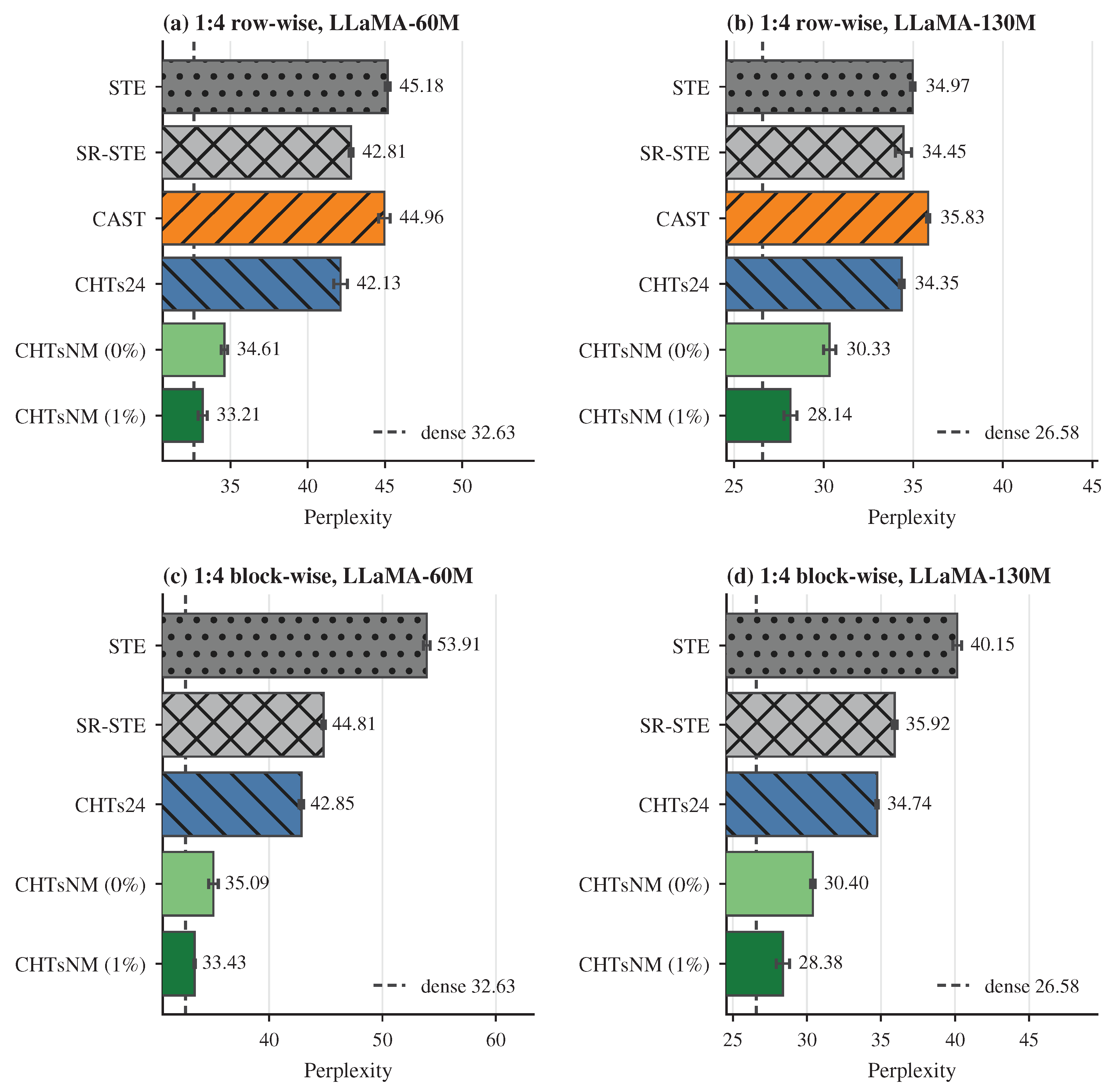
Figure A2.
Ablation of CoMoLoRA and TANS across the four sparsity-layout regimes, visualizing Table 2. Each group of four bars shows the four on/off combinations for the same regime; lower perplexity is better. TANS provides the largest single-component gain in every regime, and adding CoMoLoRA on top of TANS yields a further reduction that is largest under 1:4 sparsity.
Figure A2.
Ablation of CoMoLoRA and TANS across the four sparsity-layout regimes, visualizing Table 2. Each group of four bars shows the four on/off combinations for the same regime; lower perplexity is better. TANS provides the largest single-component gain in every regime, and adding CoMoLoRA on top of TANS yields a further reduction that is largest under 1:4 sparsity.
Appendix G. The Zero-Shot Test Result of Main Experiments
Table A5 shows the results of zero-shot tests.
Table A5.
CHTsNM achieved the best PPL and ACC in the zero-shot tasks.
| Sparsity | Method | Aux. | WikiText PPL |
LAMBADA ACC (%) |
SciQ ACC (%) |
ARC-Easy ACC (%) |
|---|---|---|---|---|---|---|
| 1:4 Row-Wise | STE | 0% | 151.17±0.50 | 8.08±0.36 | 52.17±0.25 | 31.51±0.10 |
| SR-STE | 0% | 149.01±0.89 | 7.21±0.17 | 49.70±0.35 | 31.36±0.18 | |
| CAST | 0% | 155.21±0.48 | 7.32±0.22 | 49.40±0.33 | 31.29±0.09 | |
| CHTs24 | 0% | 148.23±0.19 | 7.21±0.18 | 49.80±0.69 | 31.51±0.26 | |
| CHTsNM | 0% | 130.33±1.11 | 9.04±0.41 | 49.50±0.76 | 32.79±0.07 | |
| CHTsNM | 1% | 117.08±0.59 | 11.55±0.15 | 57.53±0.35 | 32.73±0.21 | |
| 1:4 Block-Wise | STE | 0% | 177.13±0.31 | 7.24±0.10 | 50.00±0.38 | 31.29±0.07 |
| SR-STE | 0% | 157.07±0.50 | 5.69±0.09 | 48.63±0.44 | 31.65±0.37 | |
| CHTs24 | 0% | 150.65±0.11 | 6.18±0.08 | 49.50±0.17 | 31.38±0.19 | |
| CHTsNM | 0% | 129.42±0.63 | 8.91±0.03 | 52.53±1.27 | 32.97±0.22 | |
| CHTsNM | 1% | 118.41±0.88 | 10.95±0.18 | 57.40±0.13 | 33.33±0.04 | |
| 2:4 Row-Wise | STE | 0% | 125.29±0.16 | 9.90±0.25 | 53.93±0.54 | 31.51±0.23 |
| SR-STE | 0% | 125.96±0.36 | 9.61±0.43 | 53.07±0.41 | 31.69±0.31 | |
| CAST | 0% | 128.00±0.28 | 9.79±0.17 | 52.50±0.46 | 32.01±0.14 | |
| CHTs24 | 0% | 127.05±0.42 | 10.00±0.35 | 55.37±0.60 | 32.11±0.19 | |
| CHTsNM | 0% | 107.46±0.41 | 13.13±0.17 | 57.37±0.28 | 33.35±0.11 | |
| CHTsNM | 1% | 104.08±0.10 | 14.29±0.35 | 58.77±0.20 | 33.81±0.23 | |
| 2:4 Block-Wise | STE | 0% | 135.53±0.25 | 9.57±0.04 | 53.17±0.27 | 31.48±0.16 |
| SR-STE | 0% | 128.89±0.43 | 9.21±0.13 | 53.13±0.23 | 32.01±0.19 | |
| CHTs24 | 0% | 128.41±0.40 | 9.36±0.29 | 53.77±0.24 | 32.03±0.26 | |
| CHTsNM | 0% | 108.39±0.22 | 12.65±0.25 | 59.20±0.17 | 33.99±0.04 | |
| CHTsNM | 1% | 105.09±0.18 | 13.97±0.31 | 60.57±0.70 | 33.85±0.13 |
Appendix H. Baseline Details
This note summarizes the main baseline families used in our sparse pretraining experiments. Unless otherwise stated, all methods replace the same target linear layers
Unless otherwise stated, the main sparse comparisons share the following outer training budget:
- training steps: ,
- warmup steps: ,
- sequence length: 256,
- per-device batch size: 64,
- total batch size: 256,
- final held-out evaluation: 100M tokens,
- learning rate: ,
- adam eps: ,
- weight decay: 0.
Dense anchor. The dense baseline is standard LLaMA pretraining with Adam, with no sparse projection, no DST scheduler, and no auxiliary branch.
Appendix H.1. STE
The STE[18] baseline applies a legal semi-structured mask in the forward pass, but passes the identity gradient to the underlying dense weight. If is the legal mask induced by the current weight W, then the forward uses
while the backward treats the layer as if the effective parameter were W itself. Equivalently, the autograd path is
so the optimizer receives the task gradient with no extra sparse regularization term.
Project settings. For the canonical main runs, STE is used as a direct sparse-layer replacement baseline with:
- no DST scheduler,
- Adam,
- row-wise or block-wise legal masking depending on the experiment regime.
Appendix H.2. SR-STE
SR-STE[3] keeps the same straight-through forward path as STE, but adds a regularization gradient on pruned entries. Let be the legal mask and let denote the pruned support. The task gradient is augmented by
In other words, active entries still receive the ordinary task gradient, while pruned entries are softly pushed toward zero.
Project settings. We use:
- lambda_w,
- no DST scheduler,
- the same legal row-wise or block-wise mask family as the corresponding STE run.
Appendix H.3. CAST
CAST[19] was originally proposed as a sparse training recipe with additional post-training machinery. For fairness in our pretraining comparison, we remove the teacher-distillation / KD parts and keep only the sparse-optimization core:
- the same pretraining data and token budget as the other baselines,
- the same target linear layers,
- no teacher model, no KD loss, and no extra post-training stage beyond the final sparse export.
Training-time behavior. CAST is not a sparse-forward method like STE or SR-STE. During training it keeps a dense forward weight, while sparsity only enters through two components:
- AdamS, which applies selective decay to currently pruned coordinates,
- weight scaling, which learns per-group scaling factors to compensate magnitude shrinkage.
In our implementation, the dense backbone parameters outside CAST layers are optimized normally, while CASTlinear.weight uses AdamS through a hybrid optimizer.
Final projection. At export time, CAST performs a final legal sparse projection and folds the learned scaling factors back into the weight. This is the point where the model becomes actually sparse.
Project settings. Our CAST implementation differs from plain CAST in the finalization rule: the final legal mask is computed from the scaled weight, and the finalized sparse weight is obtained by projecting that scaled weight directly.
In addition, the canonical CAST runs in this repo use:
- scaling groups,
- mask update freq,
- lambda_w,
- fp32 storage for the scaler,
- fp32 multiply for weight * scaler, then cast back for the forward path.
Why CAST is only evaluated in row-wise mode. CAST is a dense-to-sparse projection method whose final sparse structure is induced only at export time from a dense weight. Therefore, in the training process, CAST is unable to enjoy the semi-structured sparse acceleration. However, block-wise sparsity only helps to accelerate the training process. It makes no sense for CAST to test in block-wise sparsity. Accordingly, the canonical comparisons only evaluate CAST on row-wise regimes, and we do not report a block-wise CAST baseline.
Appendix H.4. CHTs24
CHTs24[13] is our legality-preserving DST backbone baseline. Unlike STE, SR-STE, or CAST, it explicitly trains a sparse backbone throughout training and updates the legal support with a structured DST scheduler.
Core idea. CHTs24 alternates between:
- structured removal on the current support, and
- legality-preserving regrowth inside the same row-wise or block-wise semi-structured regime.
This keeps the model sparse during training rather than only at export time.
Canonical settings. The main experiments use:
Appendix H.5. CHTsNM (∼1% Auxiliary Branch)
This is the main CHTsNM method. It starts from the same CHTs24 backbone, keeps TANS on the sparse backbone, and adds a small CoMoLoRA auxiliary branch (Optional).
Optimizer split. The defining implementation choice is the optimizer split:
- the sparse backbone is optimized by TANS,
- the CoMoLoRA branch is optimized by Adam.
Auxiliary-branch scale. The canonical main setting uses an approximately 1% auxiliary branch budget. Operationally, this is the “pure internal CoMoLoRA” branch added on top of a CHTs24 sparse backbone.
- Parameter budget= 1%,
- CoMoLoRA LoRA rank=7,
- Gated MLP hidden size=2,
- gamma=0.5.
Row-wise MPR variants. For row-wise follow-ups, the same MPR settings are used as above:
- row-wise 1:4: MPR forcing probability ,
- row-wise 2:4: MPR forcing probability .
TANS. The pure backbone TANS follow-up keeps the same CHTs24 topology engine but swaps the optimizer to TANS. The canonical settings are:
- lr,
- eps,
- beta1,
- beta2,
- weight decay,
- tans gamma ortho,
- refresh blend steps.
Appendix I. Additional TANS Mechanism Analysis
This appendix summarizes the parts of TANS study that are not fully exposed in the main paper tables. The mechanism suite focuses on three robustness questions: (i) how sensitive TANS is to the RMS-matching design, (ii) how much refresh ramping matters, and (iii) whether ramping can substitute for explicit optimizer-state repair after topology changes. Unless noted otherwise, all runs here use LLaMA-60M, block-wise sparsity, 10k steps, and 100M final-evaluation tokens, with two seeds per condition.
Appendix I.1. RMS-Matching Robustness Grid
Table A6 reports the RMS-matching grid . Two points stand out. First, the exact RMS-matching variant is a second-order design choice at moderate matrix-correction strength. Second, RMS matching becomes critical as the correction strength grows: at , the no-RMS variant collapses to PPL, while either RMS-matching variant recovers the result to .
Table A6.
PPL of the TANS RMS-matching robustness grid under a fixed matrix-geometry path. The main pattern is not that one RMS variant always wins, but that RMS matching becomes increasingly important as the correction strength grows.
Table A6.
PPL of the TANS RMS-matching robustness grid under a fixed matrix-geometry path. The main pattern is not that one RMS variant always wins, but that RMS matching becomes increasingly important as the correction strength grows.
| none | pre-mask global | post-mask active | |
|---|---|---|---|
| 0.25 | 34.63 | 34.95 | 35.14 |
| 0.50 | 34.61 | 34.27 | 34.51 |
| 0.75 | 35.39 | 34.57 | 34.77 |
| 1.00 | 46.72 | 36.93 | 36.93 |
The grid therefore supports a robustness claim rather than a narrow one-point optimum. TANS does not require an exact RMS-matching choice to work well, but strong matrix-geometry updates do require some form of RMS calibration to stay numerically aligned with the active sparse backbone.
Appendix I.2. Refresh-Ramp Analysis
Table A7 isolates the effect of the refresh ramp under the default topology-refresh cadence. The no-ramp baseline reaches PPL. All tested nonzero ramps are competitive, and the best tested setting is the longest one in this sweep, ramp=32, which reaches PPL. Even the shortest nonzero ramp, ramp=2, already improves over the no-ramp baseline.
Table A7.
Refresh-ramp sweep under the default dynamic-topology setting. Any nonzero ramp is at least competitive with the no-ramp baseline, and the best tested value is 32 steps.
Table A7.
Refresh-ramp sweep under the default dynamic-topology setting. Any nonzero ramp is at least competitive with the no-ramp baseline, and the best tested value is 32 steps.
| Refresh ramp | Mean PPL | vs ramp 0 |
|---|---|---|
| 0 | 34.53 | 0.00 |
| 2 | 34.17 | |
| 4 | 34.44 | |
| 8 | 34.51 | |
| 16 | 34.36 | |
| 32 | 34.12 |
The main conclusion is not that the exact best ramp value is universal, but that post-refresh softness matters. This supports the interpretation that the topology refresh introduces a genuine optimizer-transition problem, and that a gradual restoration of full matrix correction is preferable to an abrupt switch.
Appendix I.3. Optimizer-State Reset Versus Refresh Ramp
Table A8 compares no reset, changed-entry-only reset, and full-state reset, each with and without a refresh ramp. The best tested configuration is changed-entries reset + ramp=8, which reaches PPL. This is better than the corresponding no-reset setting () and also better than full-state reset with the same ramp ().
Table A8.
Optimizer-state reset versus refresh ramp. A localized reset on only the changed entries works best when combined with ramping, suggesting that the optimizer mismatch is concentrated on refreshed coordinates rather than on the whole matrix state.
Table A8.
Optimizer-state reset versus refresh ramp. A localized reset on only the changed entries works best when combined with ramping, suggesting that the optimizer mismatch is concentrated on refreshed coordinates rather than on the whole matrix state.
| State-reset mode | Ramp 0 PPL | Ramp 8 PPL |
|---|---|---|
| none | 34.53 | 34.51 |
| changed entries only | 34.50 | 34.27 |
| all state entries | 34.45 | 34.38 |
This result is mechanistically useful. It suggests that the refresh mismatch is not well modeled as a global optimizer restart problem. Instead, the damage is localized to coordinates whose sparse support status changes, so a targeted state repair is more appropriate than resetting the entire matrix state.
Appendix I.4. Summary
The extra benefit of TANS is not exhausted by the main optimizer-family ablation. Rather, the mechanism suite shows that the method remains effective across a nontrivial RMS-matching grid, benefits from explicit post-refresh softness, and is further improved by localized repair of optimizer state after topology changes. Together, these results support the view that TANS succeeds because it makes matrix-geometry optimization compatible with a changing legal sparse support, not because it depends on one fragile hyperparameter setting.
Appendix J. Optimizer Matrix Details
Table 3 isolates the mechanism underlying TANS by separating sparse preconditioning, matrix geometry, and scale control within one 1:4-active sparse setting. Table A9 evaluates the complementary optimizer-level question: whether comparable gains can be obtained by replacing AdamW with a dense matrix optimizer such as Muon. The comparison uses a matched LLaMA-130M, 10k-step training setup, and each cell reports final validation perplexity for dense training or CHTs sparse-to-sparse training at 2:4 and 1:4 sparsity.
Table A9.
PPL results of optimizer tests on LLaMA-130M PPL after 10k steps. PRE denotes preconditioned base [34] and N denotes Nesterov [35]. Lower PPL is better.
| Setting | AdamW | +PRE | +PRE+N | Muon | +PRE | +PRE+N | TANS |
|---|---|---|---|---|---|---|---|
| Dense | 30.20 | 27.98 | 27.64 | 27.29 | 27.64 | 27.24 | 26.09 |
| CHTs 2:4 | 33.85 | 31.23 | 30.86 | 31.10 | 31.79 | 31.11 | 28.52 |
| CHTs 1:4 | 38.30 | 35.41 | 35.21 | 35.70 | 36.85 | 35.90 | 32.09 |
TANS obtains the lowest PPL in all three regimes. The gain is strongest under 1:4 sparsity, where TANS reduces final PPL by relative to AdamW and relative to Muon. The same ordering holds for dense and 2:4 training: pre-conditioned base, Nesterov, and Muon-style matrix geometry improve several baselines, but they do not close the gap to TANS. This supports the interpretation that TANS is not a direct application of Muon to sparse weights; active-mask projection, active-support scale matching, and refresh-aware correction are required to make matrix geometry compatible with dynamic sparse topology.
Appendix K. Auxiliary Branch Taxonomy
This appendix provides the explicit formulas for the auxiliary-branch variants used in Section 4.4. Let denote the sparse-backbone output.
Add. This is a standard additive low-rank residual branch:
Add+Align. This variant uses the same additive low-rank branch as Add, but adds an auxiliary alignment loss which is proposed by Wu et al. [21]:
where denotes the alignment penalty and is set to .
Prod-Gate. This is a product-only contextual gate on the sparse-backbone output:
where is a lightweight gate network. This method is proposed by Zhang et al. [26]. It tests whether contextual modulation of existing sparse features alone is sufficient.
Widen. WIDEN is a capacity-control baseline without an auxiliary branch. Because the sparse backbone uses 1:4 sparsity whereas the auxiliary branch is dense, we increase the FFN width so that the number of added effective dense parameters matches the auxiliary-branch budget. It increases the FFN intermediate dimension:
CoMo. CoMoLoRA is a variant of LoRA proposed in this paper. It combines additive low-rank residual compensation with contextual rank-space product modulation:
where
The last layer of is initialized to zero, so that at initialization and CoMo starts from the standard additive low-rank branch.
Appendix L. MPR Is Not the Same as Changing zeta
We also ran a separate zeta-only control sweep without MPR. These experiments keep the model family fixed and change only the DST update-ratio . Table A10 shows that this does not behave like MPR: the sweep stays within a narrow and somewhat unstable band, whereas the row-wise MPR settings above provide a direct and interpretable improvement under the matched zeta=0.1 backbone.
Table A10.
A separatezeta-only control sweep without MPR. The effect is small and not monotone, indicating that MPR should not be interpreted as merely “using a different zeta”.
Table A10.
A separatezeta-only control sweep without MPR. The effect is small and not monotone, indicating that MPR should not be interpreted as merely “using a different zeta”.
| Setting | Regime | Seeds | Final PPL |
|---|---|---|---|
| zeta=0.10 anchor | Block-Wise 1:4 | 2 | 42.68 |
| zeta=0.05 | Block-Wise 1:4 | 2 | 42.68 |
| zeta=0.15 | Block-Wise 1:4 | 2 | 42.57 |
| zeta=0.20 | Block-Wise 1:4 | 2 | 42.80 |
| zeta=0.30 | Block-Wise 1:4 | 2 | 42.95 |
The practical takeaway is therefore narrow but clean: MPR is useful as a row-wise motif-level constraint, and its preferred strength depends on the sparsity regime. This is different from simply retuning the global DST update-ratio parameter.
Appendix M. Inference Speedup Details
Appendix M.1. Hardware and Software Setup
All measurements were collected on a single NVIDIA RTX 5080 (Blackwell) under PyTorch 2.10.0 with CUDA 12.8 and TensorRT 10.15. Both engines are compiled in BF16; the only difference is the sparse-tactic flag enabling the 2:4 sparse Tensor Core path. Each (model, shape) cell reports the mean throughput from 100 timed iterations after 20 warmup iterations, executed back-to-back on the same process and device with no other GPU workloads running. Run-to-run variance for the throughput numbers is below one percent and is therefore not shown in the table.
Appendix M.2. Measured 2:4 Speedup Protocol
The main-paper speedup result compares two BF16 inference engines built from the same trained sparse-backbone checkpoint. The dense engine treats all weights as ordinary dense tensors, while the sparse engine enables the NVIDIA 2:4 sparse Tensor Core path. This keeps model weights, precision, batch size, and sequence length fixed, so the speedup isolates the effect of legal 2:4 sparse execution.
Post-training sparsification is not applied to every matrix. The transformer projection weights keep their trained 2:4 structure, while dense components such as the embedding and output head remain dense in both engines. This evaluates a realistic sparse-transformer deployment rather than an upper bound where every linear layer is made sparse after training.
Table A11.
Full measured 2:4 inference throughput table. Throughput is reported as dense → sparse queries per second.
Table A11.
Full measured 2:4 inference throughput table. Throughput is reported as dense → sparse queries per second.
| Model | Batch 8, Seq. 128 | Batch 8, Seq. 256 | ||
|---|---|---|---|---|
| Throughput | Speedup | Throughput | Speedup | |
| LLaMA-60M | ||||
| LLaMA-130M | ||||
| LLaMA-250M | ||||
| LLaMA-350M | ||||
| LLaMA-1B | ||||
Appendix M.3. Surrogate Extrapolation from 2:4 to 1:4
The 1:4 setting is the main target of this paper, but current NVIDIA sparse Tensor Cores do not expose a native 1:4 execution mode. The 1:4 result is therefore reported as a hardware-target extrapolation rather than a measured current-hardware result.
Let and denote measured CSR runtimes for matched sparse GEMM shapes under 2:4 and 1:4 masks. CSR is used only as a relative sparsity surrogate, not as an absolute performance model. The ratio
measures the relative gain from halving the number of active values under the same sparse-matrix backend. Across the model shapes used in this surrogate study, ranges from to with mean (Figure A3). The hardware-target extrapolation is then
This treats as a first-order FLOP-scaling indicator: halving the number of active values approximately halves the arithmetic and operand traffic that a sparse-aware kernel must perform. It does not capture second-order effects such as instruction issue, scheduler behavior, or the exact memory hierarchy of a hypothetical native 1:4 Tensor Core, so the resulting target speedup should be read as a target consistent with FLOP scaling rather than as an architectural prediction.
Figure A3.
Stability of the CSR 2:4-to-1:4 runtime ratio across model shapes used in the surrogate study. The dashed line marks the mean .
Figure A3.
Stability of the CSR 2:4-to-1:4 runtime ratio across model shapes used in the surrogate study. The dashed line marks the mean .
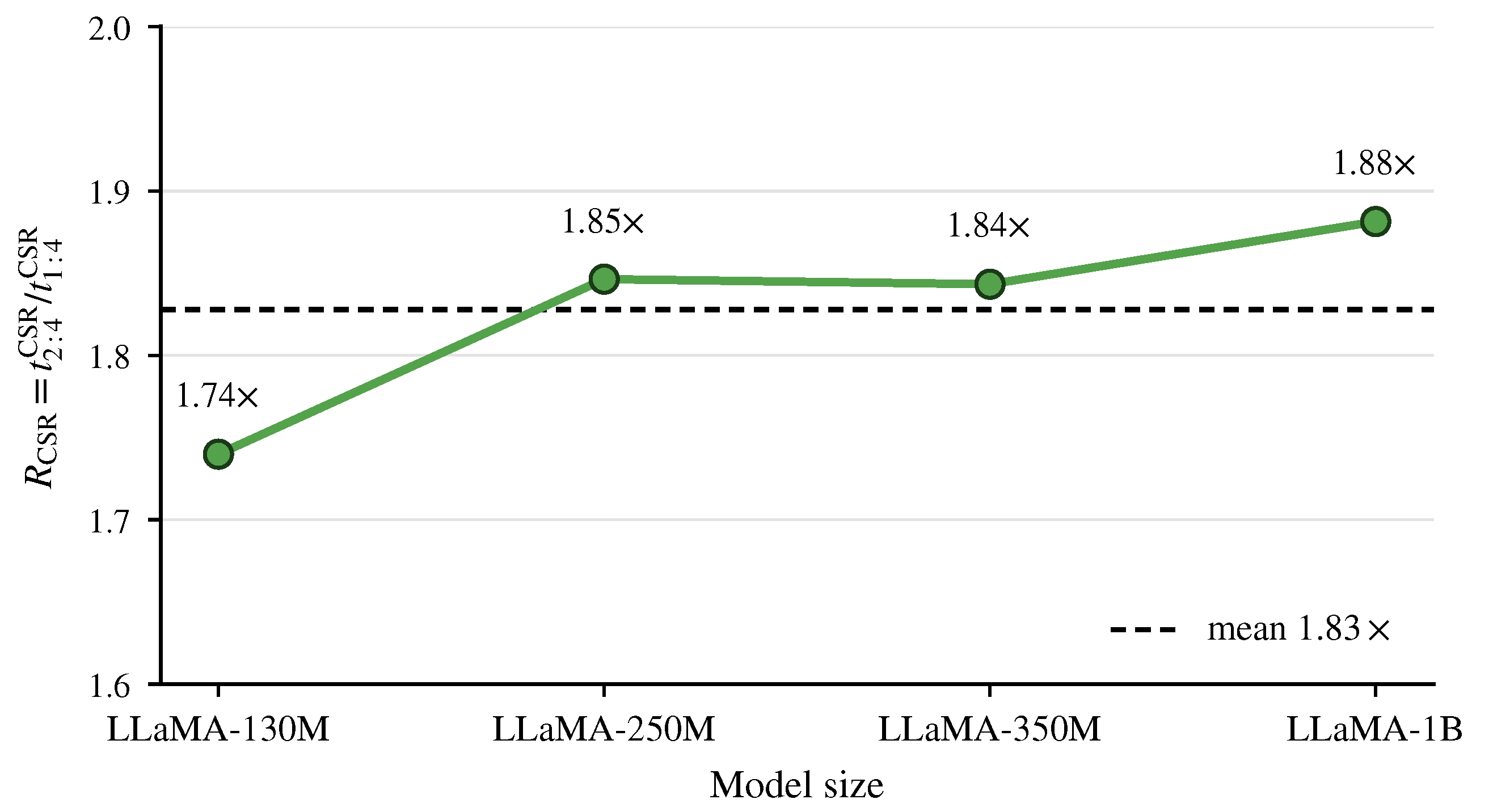
Table A12.
Surrogate extrapolation for potential native 1:4 Tensor Core inference. The 2:4 speedup column is the per-shape average from Table A11.
Table A12.
Surrogate extrapolation for potential native 1:4 Tensor Core inference. The 2:4 speedup column is the per-shape average from Table A11.
| Model | CSR ratio | Measured 2:4 speedup | Target 1:4 speedup |
|---|---|---|---|
| LLaMA-130M | |||
| LLaMA-250M | |||
| LLaMA-350M | |||
| LLaMA-1B |
Appendix M.4. Hardware-Target 1:4 Plot
Figure A4 shows the target 1:4 acceleration.
Figure A4.
Hardware-target 1:4 extrapolation. Blue bars are the per-shape averaged measured 2:4 speedups from the NVIDIA sparse Tensor Core path. Green bars multiply each measured 2:4 speedup by that model’s own (shown under the model name), not by the cross-model mean. Coverage is restricted to the model sizes for which a matched CSR surrogate measurement was available.
Figure A4.
Hardware-target 1:4 extrapolation. Blue bars are the per-shape averaged measured 2:4 speedups from the NVIDIA sparse Tensor Core path. Green bars multiply each measured 2:4 speedup by that model’s own (shown under the model name), not by the cross-model mean. Coverage is restricted to the model sizes for which a matched CSR surrogate measurement was available.
Appendix N. Limitations
Our evaluation is limited to LLaMA-style pre-training at moderate scales, with 350M as a scale-extension check. Larger models, other architectures, and downstream tasks remain to be studied. CHTsNM also adds algorithmic complexity through TANS, CoMoLoRA, and MPR. Finally, current NVIDIA hardware does not support native 1:4 sparse execution; thus, our 1:4 results should be interpreted as algorithmic evidence for a future hardware target.
Appendix N.1. Training-Side Speed and Energy
Quality results aside, we also measure the wall-clock and energy cost of one training step under the same optimizer/sparsity combinations. Each configuration runs 1000 steps of LLaMA pre-training at sequence length 256 in bf16 on a single NVIDIA RTX 5080, with concurrent pynvml power sampling for the energy and average-power numbers; see Appendix M.1 for the broader hardware and software setup.
At LLaMA-60M the per-step optimizer cost is large relative to forward and backward, so the ranking is dominated by optimizer overhead alone. We therefore report 350M, where the model contributes most of the per-step cost and the comparison better reflects realistic training; the 60M numbers behave the same way qualitatively.
Table A13 shows that TANS is slower than dense AdamW, since the orthogonalized update is substantially more expensive than an AdamW step. Against Muon the picture reverses: at every sparsity level, TANS is faster and lower-energy than the matched Muon configuration, roughly faster and about 15 to less energy, and the dense TANS run is itself already faster and lower-energy than dense Muon. Mean power is also lower for TANS than Muon in each measured comparison: vs. W for dense, vs. W for CHTs 2:4, and vs. W for CHTs 1:4. The gap is concentrated almost entirely in the optimizer step; forward and backward times differ by only a few percent across configurations.
Table A13.
LLaMA-350M training efficiency over 1000 steps, batch size 2, sequence length 256, bf16, RTX 5080. Energy is normalized as joules per token.
Table A13.
LLaMA-350M training efficiency over 1000 steps, batch size 2, sequence length 256, bf16, RTX 5080. Energy is normalized as joules per token.
| Setting | Step time | Opt. step | Throughput | J / token |
|---|---|---|---|---|
| Dense AdamW | 248.19 ms | 16.89 ms | 2,025 tok/s | 0.0893 |
| Dense Muon | 354.82 ms | 124.46 ms | 1,419 tok/s | 0.1336 |
| Dense TANS | 315.43 ms | 84.53 ms | 1,595 tok/s | 0.1083 |
| CHTs 2:4 + TANS | 328.26 ms | 96.22 ms | 1,533 tok/s | 0.1157 |
| CHTs 2:4 + Muon | 366.93 ms | 133.58 ms | 1,373 tok/s | 0.1402 |
| CHTs 1:4 + TANS | 331.84 ms | 98.43 ms | 1,517 tok/s | 0.1130 |
| CHTs 1:4 + Muon | 367.18 ms | 133.56 ms | 1,372 tok/s | 0.1376 |
References
- Mishra, A.; Latorre, J.A.; Pool, J.; Stosic, D.; Stosic, D.; Venkatesh, G.; Yu, C.; Micikevicius, P. Accelerating sparse deep neural networks. arXiv 2021, arXiv:2104.08378. [Google Scholar] [CrossRef]
- Nvidia. A100 Tensor Core GPU Architecture. 2020. Available online: https://www.nvidia.com/content/dam/en-zz/Solutions/Data-Center/nvidia-ampere-architecture-whitepaper.pdf (accessed on 2026-05-01).
- Zhou, A.; Ma, Y.; Zhu, J.; Liu, J.; Zhang, Z.; Yuan, K.; Sun, W.; Li, H. Learning n: m fine-grained structured sparse neural networks from scratch. International Conference on Learning Representations 2021. [Google Scholar]
- Yao, Z.; Cao, S.; Xiao, W.; Zhang, C.; Nie, L. Balanced sparsity for efficient dnn inference on gpu. Proc. AAAI Conf. Artif. Intell. 2019, 33, 5676–5683. [Google Scholar] [CrossRef]
- Wu, S.; Li, G.; Chen, F.; Shi, L. Training and inference with integers in deep neural networks. International Conference on Learning Representations 2018. [Google Scholar]
- Wang, N.; Choi, J.; Brand, D.; Chen, C.Y.; Gopalakrishnan, K. Training deep neural networks with 8-bit floating point numbers. Adv. Neural Inf. Process. Syst. 2018, 31. [Google Scholar]
- Zhu, F.; Gong, R.; Yu, F.; Liu, X.; Wang, Y.; Li, Z.; Yang, X.; Yan, J. Towards unified int8 training for convolutional neural network. Proceedings of the IEEE/CVF Conference on Computer Vision and Pattern Recognition 2020, 1969–1979. [Google Scholar]
- Nvidia, *!!! REPLACE !!!*. Floating-Point 8: An Introduction to Efficient, Lower-Precision AI Training. 2025. Available online: https://developer.nvidia.com/blog/floating-point-8-an-introduction-to-efficient-lower-precision-ai-training/ (accessed on 2026-05-01).
- Hu, Y.; Zhu, J.; Chen, J. S-ste: Continuous pruning function for efficient 2: 4 sparse pre-training. Adv. Neural Inf. Process. Syst. 2024, 37, 33756–33778. [Google Scholar]
- Hu, E.J.; shen, yelong; Wallis, P.; Allen-Zhu, Z.; Li, Y.; Wang, S.; Wang, L.; Chen, W. LoRA: Low-Rank Adaptation of Large Language Models. International Conference on Learning Representations 2022. [Google Scholar]
- Liu, J.; Su, J.; Yao, X.; Jiang, Z.; Lai, G.; Du, Y.; Qin, Y.; Xu, W.; Lu, E.; Yan, J.; et al. Muon is scalable for llm training. arXiv 2025, arXiv:2502.16982. [Google Scholar] [CrossRef]
- Bengio, Y.; Léonard, N.; Courville, A. Estimating or propagating gradients through stochastic neurons for conditional computation. arXiv 2013, arXiv:1308.3432. [Google Scholar] [CrossRef]
- Lyu, J.; Wang, R.; Bao, K.; Zhang, Y.; Cannistraci, C.V. Cannistraci-Hebb Training with N: M Semi-Structured Sparsity for Pre-Training and Re-Training. Conference on Parsimony and Learning 2026. [Google Scholar]
- Houlsby, N.; Giurgiu, A.; Jastrzebski, S.; Morrone, B.; De Laroussilhe, Q.; Gesmundo, A.; Attariyan, M.; Gelly, S. Parameter-efficient transfer learning for NLP. International conference on machine learning 2019, 2790–2799. [Google Scholar]
- Jordan, K.; Jin, Y.; Boza, V.; You, J.; Cesista, F.; Newhouse, L.; Bernstein, J. Muon: An optimizer for hidden layers in neural networks. 2024. Available online: https://kellerjordan.github.io/posts/muon/ (accessed on 2026-05-01).
- Bernstein, J.; Newhouse, L. Modular Duality in Deep Learning. International Conference on Machine Learning 2025. [Google Scholar]
- Touvron, H.; Lavril, T.; Izacard, G.; Martinet, X.; Lachaux, M.A.; Lacroix, T.; Rozière, B.; Goyal, N.; Hambro, E.; Azhar, F.; et al. Llama: Open and efficient foundation language models. arXiv 2023, arXiv:2302.13971. [Google Scholar] [CrossRef]
- Hu, Y.; Zhao, K.; Huang, W.; Chen, J.; Zhu, J. Accelerating transformer pre-training with 2: 4 sparsity. International Conference on Machine Learning 2024. [Google Scholar]
- Huang, W.; Hu, Y.; Zhu, J.; Chen, J. CAST: Continuous and Differentiable Semi-Structured Sparsity-Aware Training for Large Language Models. arXiv 2025, arXiv:2509.25996. [Google Scholar]
- Hubara, I.; Chmiel, B.; Island, M.; Banner, R.; Naor, J.; Soudry, D. Accelerated sparse neural training: A provable and efficient method to find n: m transposable masks. Adv. Neural Inf. Process. Syst. 2021, 34, 21099–21111. [Google Scholar]
- Wu, W.; Zhang, Y.; Zhao, J.; Cannistraci, C.V. Alignment-Enhanced Integration of Connectivity and Spectral Sparsity in Dynamic Sparse Training of LLM. International Conference on Learning Representations 2026. [Google Scholar]
- Han, A.; Li, J.; Huang, W.; Hong, M.; Takeda, A.; Jawanpuria, P.; Mishra, B. SLTrain: a sparse plus low rank approach for parameter and memory efficient pretraining. Adv. Neural Inf. Process. Syst. 2024, 37, 118267–118295. [Google Scholar]
- Makni, M.; Behdin, K.; Xu, Z.; Ponomareva, N.; Mazumder, R. Hassle-free: A unified framework for sparse plus low-rank matrix decomposition for llms. arXiv 2025, arXiv:2502.00899. [Google Scholar]
- Mozaffari, M.; Yazdanbakhsh, A.; Zhang, Z.; Dehnavi, M.M. Slope: Double-pruned sparse plus lazy low-rank adapter pretraining of llms. International Conference on Learning Representations 2025. [Google Scholar]
- Liu, L.; Liu, A.; Wang, M.; Zhao, T.; Yang, L.F. ARMOR: High-Performance Semi-Structured Pruning via Adaptive Matrix Factorization. International Conference on Learning Representations 2026. [Google Scholar]
- Zhang, Y.; Gu, W.; Hu, W.; Li, J.; Cannistraci, C.V. From Transformer to Transponder: Introducing Contextual Modulation Training for Residual Learning in LLMs. Preprints 2025. [Google Scholar] [CrossRef]
- Merity, S.; Xiong, C.; Bradbury, J.; Socher, R. Pointer Sentinel Mixture Models. International Conference on Learning Representations 2017. [Google Scholar]
- Paperno, D.; Kruszewski, G.; Lazaridou, A.; Pham, N.Q.; Bernardi, R.; Pezzelle, S.; Baroni, M.; Boleda, G.; Fernández, R. The LAMBADA dataset: Word prediction requiring a broad discourse context. Proc. 54th Annu. Meet. Assoc. Comput. Linguist. 2016, volume 1, 1525–1534. [Google Scholar]
- Welbl, J.; Liu, N.F.; Gardner, M. Crowdsourcing multiple choice science questions. Proceedings of the 3rd Workshop on Noisy User-generated Text 2017, 94–106. [Google Scholar]
- Clark, P.; Cowhey, I.; Etzioni, O.; Khot, T.; Sabharwal, A.; Schoenick, C.; Tafjord, O. Think you have solved question answering? try arc, the ai2 reasoning challenge. arXiv 2018, arXiv:1803.05457. [Google Scholar] [CrossRef]
- Gokaslan, A.; Cohen, V. OpenWebText Corpus. 2019. Available online: http://Skylion007.github.io/OpenWebTextCorpus.
- Zhang, Y.; Zhao, J.; Wu, W.; Muscoloni, A. Epitopological learning and cannistraci-hebb network shape intelligence brain-inspired theory for ultra-sparse advantage in deep learning. International Conference on Learning Representations 2024. [Google Scholar]
- Zhang, Y.; Cerretti, D.; Zhao, J.; Wu, W.; Liao, Z.; Michieli, U.; Cannistraci, C.V. Brain network science modelling of sparse neural networks enables Transformers and LLMs to perform as fully connected. Advances in Neural Information Processing Systems 2025. [Google Scholar]
- Ziyin, L.; Wang, Z.T.; Ueda, M. LaProp: Separating momentum and adaptivity in Adam. arXiv 2020, arXiv:2002.04839. [Google Scholar]
- Dozat, T. Incorporating nesterov momentum into adam. International Conference on Learning Representations 2016. [Google Scholar]
Table 1.
Under 1:4 sparsity, CHTsNM delivers near-dense performance. We compare CHTsNM with all baselines on LLaMA-60M and LLaMA-130M. PPL denotes perplexity on OpenWebText [31]. Under 1:4 sparsity, CHTsNM reduces PPL by 21.6% and 18.2%, respectively. Under 2:4 sparsity, CHTsNM can even outperform the dense model without using the LoRA branch. This trend is further confirmed on LLaMA-350M. Boldface indicates the best result, and PPL * denotes a PPL lower than that of the dense model.
Table 1.
Under 1:4 sparsity, CHTsNM delivers near-dense performance. We compare CHTsNM with all baselines on LLaMA-60M and LLaMA-130M. PPL denotes perplexity on OpenWebText [31]. Under 1:4 sparsity, CHTsNM reduces PPL by 21.6% and 18.2%, respectively. Under 2:4 sparsity, CHTsNM can even outperform the dense model without using the LoRA branch. This trend is further confirmed on LLaMA-350M. Boldface indicates the best result, and PPL * denotes a PPL lower than that of the dense model.
| LLaMA Model Size | 60M | 130M | 350M | |||
|---|---|---|---|---|---|---|
| Sparsity | Method | Aux. Param. | PPL | PPL | PPL | |
| Dense | 0% | 32.63 ± 0.09 | 26.58 ± 0.05 | 18.09 | ||
| 1:4 | Row-Wise | STE | 0% | 45.18 ± 0.09 | 34.97 ± 0.07 | - |
| SR-STE | 0% | 42.81 ± 0.07 | 34.45 ± 0.26 | - | ||
| CAST | 0% | 44.96 ± 0.22 | 35.83 ± 0.05 | - | ||
| CHTs24 | 0% | 42.13 ± 0.26 | 34.35 ± 0.08 | - | ||
| CHTsNM | 0% | 34.61 ± 0.12 | 30.33 ± 0.20 | - | ||
| CHTsNM | 1% | 33.21 ± 0.18 | 28.14 ± 0.21 | - | ||
| Block-wise | STE | 0% | 53.91 ± 0.17 | 40.15 ± 0.17 | - | |
| SR-STE | 0% | 44.81 ± 0.08 | 35.92 ± 0.09 | - | ||
| CHTs24 | 0% | 42.85 ± 0.12 | 34.74 ± 0.04 | - | ||
| CHTsNM | 0% | 35.09 ± 0.25 | 30.40 ± 0.09 | - | ||
| CHTsNM | 1% | 33.43 ± 0.04 | 28.38 ± 0.27 | - | ||
| 2:4 | Row-wise | STE | 0% | 37.28 ± 0.15 | 29.72 ± 0.03 | - |
| SR-STE | 0% | 36.39 ± 0.06 | 29.65 ± 0.05 | - | ||
| CAST | 0% | 37.29 ± 0.13 | 30.04 ± 0.01 | - | ||
| CHTs24 | 0% | 36.61 ± 0.04 | 29.98 ± 0.05 | - | ||
| CHTsNM | 0% | 30.60 ± 0.04 * | 26.21 ± 0.05 * | - | ||
| CHTsNM | 1% | 30.51 ± 0.09 * | 25.57 ± 0.02 * | - | ||
| Block-wise | STE | 0% | 40.81 ± 0.13 | 31.83 ± 0.04 | - | |
| SR-STE | 0% | 37.26 ± 0.05 | 30.14 ± 0.10 | - | ||
| CHTs24 | 0% | 37.15 ± 0.01 | 30.12 ± 0.04 | 18.46 | ||
| CHTsNM | 0% | 30.89 ± 0.06 * | 26.50 ± 0.03 * | 16.97 * | ||
| CHTsNM | 1% | 30.45 ± 0.05 * | 25.71 ± 0.05 * | - | ||
Table 2.
TANS provides the dominant gain, while CoMoLoRA gives a complementary improvement that is larger under 1:4 sparsity. The ablation test is done on LLaMA-60M. PPL denotes perplexity on OpenWebText [31].
Table 2.
TANS provides the dominant gain, while CoMoLoRA gives a complementary improvement that is larger under 1:4 sparsity. The ablation test is done on LLaMA-60M. PPL denotes perplexity on OpenWebText [31].
| CoMoLoRA | TANS | 1:4 | 2:4 | ||
|---|---|---|---|---|---|
| Block-Wise | Row-Wise | Block-Wise | Row-Wise | ||
| – | – | 42.85 ± 0.14 | 42.03 ± 0.20 | 37.15 ± 0.02 | 36.61 ± 0.13 |
| – | ✓ | 35.09 ± 0.31 | 34.61 ± 0.14 | 30.89 ± 0.08 | 30.60 ± 0.05 |
| ✓ | – | 39.74 ± 0.16 | 38.97 ± 0.08 | 35.84 ± 0.04 | 35.31 ± 0.03 |
| ✓ | ✓ | 33.43 ± 0.05 | 33.21 ± 0.26 | 30.45 ± 0.08 | 30.51 ± 0.13 |
Table 3.
Making matrix geometry compatible with 1:4-active sparse training. Variants are named by the design principle they test.
Table 3.
Making matrix geometry compatible with 1:4-active sparse training. Variants are named by the design principle they test.
| Variant | Sparse base | Matrix geom. | Scale ctrl. | PPL ↓ |
|---|---|---|---|---|
| AdamW | – | – | – | 42.74 |
| Geometry matrix update | – | ✓ | – | 47.40 |
| Sparse preconditioned base | ✓ | – | – | 35.29 |
| Topology-agnostic NS correction | ✓ | ✓ | – | 34.78 |
| Scale-calibrated NS correction | ✓ | ✓ | ✓ | 34.55 |
| TANS | ✓ | ✓ | ✓ | 34.29 |
Table 4.
The PPL of different auxiliary-branch design under a block-wise 1:4 CHTs24 backbone on LLaMA-60M. With a parameter budget ranging from 2% to 5%, CoMoLoRA performs the best.
Table 4.
The PPL of different auxiliary-branch design under a block-wise 1:4 CHTs24 backbone on LLaMA-60M. With a parameter budget ranging from 2% to 5%, CoMoLoRA performs the best.
| Budget | 1% | 2% | 3% | 4% | 5% |
|---|---|---|---|---|---|
| Widen | 42.21 ± 0.12 | 41.84 ± 0.27 | 41.53 ± 0.15 | 40.92 ± 0.26 | 40.5 ± 0.12 |
| Add | 39.73 ± 0.02 | 38.74 ± 0.18 | 38.44 ± 0.31 | 37.58 ± 0.26 | 37.15 ± 0.03 |
| Add+Align | 39.61 ± 0.07 | 38.75 ± 0.18 | 38.34 ± 0.14 | 37.51 ± 0.05 | 37.28 ± 0.07 |
| Prod-Gate | 41.86 ± 0.49 | 41.2 ± 0.08 | 41.13 ± 0.35 | 40.87 ± 0.38 | 40.31 ± 0.13 |
| CoMoLoRA | 39.72 ± 0.22 | 38.69 ± 0.07 | 37.77 ± 0.3 | 37.45 ± 0.01 | 36.85 ± 0.06 |
Table 5.
Measured CHTsNM inference speedup on trained LLaMA sparse-backbone checkpoints.
| Shape | 60M | 130M | 250M | 350M | 1B |
|---|---|---|---|---|---|
| Batch 8, Seq. 128 | |||||
| Batch 8, Seq. 256 |
Disclaimer/Publisher’s Note: The statements, opinions and data contained in all publications are solely those of the individual author(s) and contributor(s) and not of MDPI and/or the editor(s). MDPI and/or the editor(s) disclaim responsibility for any injury to people or property resulting from any ideas, methods, instructions or products referred to in the content. |
© 2026 by the authors. Licensee MDPI, Basel, Switzerland. This article is an open access article distributed under the terms and conditions of the Creative Commons Attribution (CC BY) license (http://creativecommons.org/licenses/by/4.0/).
Copyright: This open access article is published under a Creative Commons CC BY 4.0 license, which permit the free download, distribution, and reuse, provided that the author and preprint are cited in any reuse.


