
Submitted:
07 May 2026
Posted:
12 May 2026
You are already at the latest version
Abstract
Multimodal reinforcement learning agents must fuse signals with vastly different noise profiles—yet existing architectures, whether monolithic (π0, DreamerV3) or modular (MSDP, VTDexManip), allow noise from unreliable modalities to contaminate reliable ones at the point of fusion. We propose filter-before-mixing: each modality’s representation is independently refined by a per-modality Flow Matching module before spectral-domain fusion via a Fourier Neural Operator (FNO), with a residual gate ensuring that refinement is never harmful. The resulting architecture, FreamerV1 (Filter-before-mixing dreamer), has 93M parameters (0.4M trainable). On MiniGrid, FreamerV1 reaches 100% success at 5000 episodes, surpassing the 94% encoder-only baseline which degrades to 78% due to catastrophic forgetting. On Crafter (no language modality), it scores 16.0%, exceeding DreamerV3 (14.5%). On PAMAP2 wearable sensors—where no pre-trained encoder exists—the foundation encoder achieves 2.4× higher reward and 16× lower variance than a vanilla MLP, confirming that the filter-before-mixing advantage grows with encoder noise.
Keywords:
multimodal reinforcement learning
; per-modality denoising
; flow matching
; fourier neural operator
; spectral fusion
; slot attention
; catastrophic forgetting
; wearable health management
; world model
; episodic memory
1. Introduction
Reinforcement learning agents operating in the physical world receive information through multiple sensors: cameras capture spatial structure, proprioceptive sensors report joint angles, language instructions convey goals, and reward signals provide sparse feedback. These modalities differ vastly in noise level, sampling rate, and information density. A robust multimodal RL system must combine them without allowing noise from one channel to degrade the others.
Recent RL architectures address multimodal fusion in two broad ways. Monolithic approaches process all modalities through a single shared backbone. DreamerV3 [1] feeds observations through a shared encoder–RSSM pipeline with fixed hyperparameters, mastering over 150 tasks spanning Atari to robotic control. 0 [2] tokenizes vision, language, state, and action noise into a 3B-parameter PaliGemma transformer with flow matching for continuous action generation. Genie 2 [3] and DIAMOND [4] apply diffusion to world model prediction and video generation respectively. These systems rely on model scale to implicitly absorb distributional differences across modalities.
Modular approaches assign a dedicated encoder to each modality, then fuse the outputs. MSDP [5] pretrains a multisensory encoder via masked autoencoding across vision, force, and proprioception, then fuses embeddings through cross-attention. VTDexManip [6] concatenates CLIP visual features with tactile MLP features for dexterous manipulation, finding that adding sparse touch signals improves success rates by 20%. MIB [7] compresses a joint representation via the information bottleneck principle, filtering task-irrelevant information after fusion. These methods use separate encoders but do not equalize signal quality before fusion: the noisy output of a sparse reward encoder enters the same fusion layer as a well-encoded CLIP embedding.
Both paradigms thus share a common vulnerability: cross-modal noise contamination at the point of fusion. When a high-variance modality (e.g., sparse reward, raw IMU acceleration) is fused with a low-variance one (e.g., CLIP vision embedding), noise from the former can corrupt the latter. This problem is especially acute in sensor-driven domains such as wearable health management, where modalities have radically different noise profiles and temporal scales—physical movement precedes heart-rate elevation by several seconds, and language instructions precede visual confirmation by many steps.
A second gap is the absence of principled spectral-domain fusion. Standard attention computes instantaneous pairwise similarities and cannot naturally represent temporally delayed cross-modal correlations. A third gap is the limited application to healthcare. MedDreamer [8] applied an RSSM to electronic health records, and KANDI [9] used diffusion policies for elderly activity promotion, but no prior work has combined per-modality generative refinement with spectral fusion for wearable-sensor health intervention.
This paper addresses these gaps through a design principle we call filter-before-mixing: each modality’s representation is independently refined by a dedicated Flow Matching module before cross-modal fusion, analogous to the signal processing practice of filtering each channel before mixing into a master bus. The refinement intensity adapts to each modality’s signal quality: weak for already well-encoded signals (e.g., frozen CLIP embeddings) and strong for noisy or sparse signals (e.g., raw reward, IMU data). The refined representations are then fused in the spectral domain via a Fourier Neural Operator (FNO), whose complex-valued weights naturally encode phase-shifted cross-modal correlations. An information-theoretic analysis (Section 3.3) shows that pre-fusion denoising preserves more policy-relevant mutual information than post-fusion alternatives, with a residual gate mechanism ensuring that the refinement is never harmful.
The resulting four-layer modular architecture integrates modality-specific encoding (frozen CLIP with Slot Attention, or IMU foundation encoders for health applications), per-modality Flow Matching, FNO spectral fusion, and DNC episodic memory. The modular design enables domain transfer: the same downstream pipeline (Flow Matching → FNO → DNC → PPO) is shared between MiniGrid navigation and PAMAP2 health management, with only the modality-specific encoders replaced.
We validate the framework in three domains. In MiniGrid navigation, the system achieves 94.0% success on MultiRoom-N2-S4 (+51 pp over IMPALA under identical conditions) and 93.0% on N4-S4, while IMPALA fails entirely on harder configurations (0% on N4-S5 and N6). In Crafter, a procedurally generated open-world environment with no language instructions, the agent achieves an official score of 16.0%, exceeding DreamerV3 (14.5%) despite operating without the language modality. In wearable-sensor health management on the PAMAP2 dataset—where no pre-trained encoder exists and per-modality denoising is critical—the foundation encoder achieves 2.4× higher cumulative reward () and 16× lower cross-seed variance than a vanilla MLP baseline. This progression—MiniGrid (4 modalities, CLIP available), Crafter (3 modalities, no language), PAMAP2 (3 modalities, no pre-trained encoder)—illustrates a key insight: the advantage of filter-before-mixing grows with encoder noise and is robust to missing modalities.
The contributions of this paper are as follows:
- 1.
- We propose the filter-before-mixing design principle for multimodal RL, in which per-modality Flow Matching denoises each representation before spectral-domain fusion, and provide an information-theoretic justification with an explicit approximation bound (Eq. (A11)).
- 2.
- We instantiate this principle in FreamerV1 (Filter-before-mixing dreamer), a modular four-layer architecture (93M parameters, 0.4M trainable), and validate it on MiniGrid navigation with controlled baselines (IMPALA under identical conditions, PPO).
- 3.
- We validate across three domains—MiniGrid (4 modalities), Crafter (3 modalities, no language), and PAMAP2 (3 modalities, no pre-trained encoder)—showing that the architecture degrades gracefully with missing modalities and that the filter-before-mixing advantage grows with encoder noise.
Table 1 summarizes how these design choices differentiate FreamerV1 from 0. These are not claims of superiority; they reflect optimization for a different regime—sensor-driven decision-making with discrete actions, limited data, and the need for interpretable, modular policies.
2. Related Work
We organize related work along the three problems identified in the Introduction: (1) how existing architectures fuse multimodal inputs and where cross-modal noise contamination arises, (2) how generative models have been applied in RL and where our per-modality approach diverges, and (3) how world models have been used in healthcare.
2.1. Multimodal Fusion in RL Foundation Models
The dominant approach to multimodal fusion in recent RL foundation models is monolithic: all modalities are tokenized and processed by a single large transformer. 0 [2] feeds image tokens (from PaliGemma), language tokens, robot-state tokens, and noisy action tokens into a shared self-attention backbone, relying on the model’s 3B-parameter capacity to implicitly disentangle heterogeneous inputs. Gato [10] similarly serializes text, images, and actions into a single token sequence for a 1.2B-parameter transformer. DreamerV3 [1] fuses observations through a shared encoder–RSSM pipeline with fixed hyperparameters across both discrete and continuous action domains, achieving human-level Atari performance and competitive robotic control.
These architectures have proven effective when the input modalities are relatively homogeneous (e.g., images and proprioception in robotic manipulation) or when the model is large enough to absorb distributional differences. However, they do not explicitly prevent noise from one modality from propagating to another during fusion—the problem we term cross-modal noise contamination. Our framework addresses this by denoising each modality independently via per-modality Flow Matching before fusion.
A related line of work explores modality-specific processing. CLIP [11] demonstrated the power of separate vision and language encoders aligned through contrastive learning. Slot Attention [12] decomposes visual inputs into object-centric slots, enabling structured representation learning. SAVi [13] extended this to video with temporally consistent slot tracking. We adopt both CLIP and Slot Attention as modality-specific encoders in Layer 1 of our architecture, using them as established building blocks rather than claiming novelty for their individual designs.
2.1.1. Multimodal Sensor Fusion in RL
Recent work has increasingly recognized that naive fusion of heterogeneous sensor modalities can degrade RL performance. Meng et al. [7] demonstrated that concatenating egocentric images and proprioception can fail to match single-modality performance, and proposed a Multimodal Information Bottleneck (MIB) that compresses joint representations while retaining task-relevant information. Their approach filters out task-irrelevant information after fusion, in contrast to our per-modality pre-fusion denoising.
In contact-rich robotic manipulation, MSDP [5] proposed self-supervised multisensory pretraining using masked autoencoding across vision, force, and proprioception. Their key insight is an asymmetric actor-critic architecture: the critic uses cross-attention over frozen sensor embeddings for dynamic feature extraction, while the actor receives a stable pooled representation. This achieves robustness to sensor noise with as few as 6,000 online interactions on real hardware. However, MSDP does not apply modality-specific noise reduction before fusion—all sensor embeddings enter the same transformer encoder and are masked uniformly.
VTDexManip [6] presented a benchmark for visual-tactile dexterous manipulation, comparing 17 pretrained and non-pretrained methods. Their results showed that adding sparse binary tactile signals to vision improves success rates by approximately 20%, and joint visual-tactile pretraining gains a further 20%. Fusion is achieved by concatenating visual features (from CLIP, R3M, or ResNet) with tactile MLP features—a simple strategy that does not account for the very different noise characteristics of high-resolution images versus sparse binary contact signals.
These approaches share a common pattern: modality-specific encoders followed by concatenation, cross-attention, or information-theoretic fusion. None applies generative refinement (e.g., Flow Matching) to individual modality representations before fusion. Our per-modality FM fills this gap by allowing the refinement intensity to be tuned per modality—weak for already well-encoded signals (e.g., CLIP vision) and strong for noisy or sparse signals (e.g., reward, raw IMU)—before spectral fusion combines the cleaned representations.
2.2. Generative Models and Memory in RL
Generative models in RL have been applied almost exclusively at the output stage: Decision Diffuser [14] generates trajectories, Diffusion Policy [15] produces action chunks, 0 [2] applies flow matching to 50-step action generation, and DIAMOND [4] learns world models via diffusion over observations. All operate after multimodal fusion. Our approach inverts this: Flow Matching operates on internal representations before fusion, refining each modality’s encoding via learned optimal transport. For fusion itself, we employ a Fourier Neural Operator (FNO) [16], whose complex-valued spectral weights naturally encode phase-shifted cross-modal correlations—a property absent from attention-based fusion.
2.3. World Models: From Games to Healthcare
World models—learned environment simulators that predict future states from actions—have become a dominant paradigm for sample-efficient RL. DreamerV2 [19] introduced categorical latent representations for discrete-action Atari games. DreamerV3 [1] generalized this across 150+ tasks with fixed hyperparameters, spanning Atari, DMControl, Minecraft, and Crafter, handling both discrete and continuous actions. MuZero [20] combined learned models with Monte Carlo tree search for board games and Atari. More recently, DIAMOND [4] and Genie 2 [3] have explored diffusion-based world models at foundation scale.
Despite this success, world model-based RL remains underexplored in healthcare. MedDreamer [8] is the closest precedent: it adapts the DreamerV3 RSSM to electronic health records (EHRs) for sepsis treatment and mechanical ventilation, introducing an Adaptive Feature Integration module to handle irregular clinical time series. KANDI [9] addresses physical activity promotion for fall-risk elderly using wearable accelerometers, combining Diffusion Policies with offline inverse RL. However, neither MedDreamer nor KANDI employs structured multimodal encoding (Slot Attention, per-modality Flow Matching) or spectral-domain fusion, and neither targets continuous wearable-sensor health management with online imagination-based policy optimization.
2.4. Positioning of This Work
Table 2 positions our framework against existing methods along five capability axes that correspond to the design choices motivated in the Introduction. No prior method combines per-modality generative representation refinement, spectral-domain cross-modal fusion, language-grounded reward shaping, external episodic memory, and world model-based health intervention.
3. Proposed Method
This section describes the architecture that instantiates the filter-before-mixing principle introduced in Section I.
3.1. Architecture Overview
The architecture consists of four layers (Figure 1):
- 1.
- Layer 1 — Modality-Specific Encoding. Each of four input modalities (state, vision, language, reward) is encoded by a dedicated module. Vision uses a frozen CLIP ViT-B/32 [11] with Slot Attention [12]; language uses a Transformer encoder [21] with Slot Attention; state uses an FNO-based encoder [16]; reward uses a temporal Conv1D encoder. All encoders produce d-dimensional embeddings.
- 2.
- Layer 2 — Per-Modality Flow Matching. Each modality embedding is refined by an independent Flow Matching module [22] that learns an optimal transport map from a Gaussian prior to the modality’s data manifold, denoising the representation before cross-modal fusion.
- 3.
- Layer 3 — FNO Spectral Fusion. The refined modality embeddings are stacked as a matrix and fused via spectral-domain convolution [16] (SpectralConv1d), producing a unified representation.
- 4.
The total parameter count is 93.05M, of which 92.68M (99.6%) are the frozen CLIP encoder. The trainable parameters amount to 0.37M, enabling efficient learning on small datasets.
3.2. Layer 1: Modality-Specific Encoding
Each modality is encoded by a dedicated module producing a d-dimensional embedding (details in Appendix E).
For vision, a frozen CLIP ViT-B/32 [11] extracts 49 patch features ( grid, 768-dim), projected to . Slot Attention [12] decomposes the features into K object-centric slots via iterative competitive assignment. Four numerical stabilization techniques reduce the NaN occurrence rate from 23.5% to 0% (Table 5).
For language, the mission text is processed by a Transformer encoder and decomposed into slots via Slot Attention. An LLM (Qwen2.5 [24]) parses the mission into structured components for reward shaping (Appendix A).
For state, the MiniGrid observation () is flattened and encoded by a 1D FNO block [16].
For reward, the past H-step reward history is encoded by a temporal Conv1D.
Bidirectional multi-head cross-modal attention between visual and language slots enables component-level correspondence (e.g., “green goal” slot ↔ green object slot). The resulting slots are mean-pooled to produce modality embeddings .
3.3. Layer 2: Per-Modality Flow Matching
For each modality , we apply an independent Flow Matching module to refine the encoded representation before cross-modal fusion. This implements the “filter-before-mixing” principle (Section III-A-2).
Each module learns a velocity field via Conditional Flow Matching (CFM) [22] and refines by Euler integration from to over N steps (see Appendix E for the full formulation):
A learnable residual gate ensures training stability:
where is initialized to so that at the start of training, ensuring that the FM module acts as a near-identity function until its velocity field is sufficiently trained. Crucially, the refinement intensity can be set independently per modality: weak for already well-encoded signals (e.g., frozen CLIP: , ) and strong for noisy signals (e.g., sparse reward: , ).
We provide an information-theoretic argument for why applying Flow Matching to each modality independently before fusion is preferable to applying it after fusion (see Appendix J for the full derivation).
Let denote the encoded representations of M modalities, each corrupted by modality-specific noise: , where and the noise variances differ across modalities.
In post-fusion denoising (as in 0), the noisy representations are first fused as and then denoised. By the data processing inequality [25], information lost during noisy fusion cannot be recovered. Cross-modal noise propagates through shared projection weights.
In pre-fusion denoising (our approach), a modality-specific denoiser is applied to obtain , then the cleaned representations are fused. If each FM achieves near-optimal denoising:
In practice, the FM modules are imperfect denoisers with error . Pre-fusion denoising remains beneficial whenever —a condition substantially weaker than optimal denoising (see Appendix J for the full derivation). The residual gate further tightens this bound: since when the velocity field is untrained, pre-fusion denoising is never worse than no denoising.
3.4. Layer 3: FNO Spectral Fusion
The four refined modality embeddings are stacked into a matrix and fused via a Fourier Neural Operator (FNO) [16]. The FNO applies spectral convolution: FFT along the embedding dimension, multiplication by learnable complex-valued weights for the first K Fourier modes, and inverse FFT, with a pointwise residual path (see Appendix E for the full formulation). The fused representation is obtained by mean-pooling over the modality axis.
The key advantage of spectral-domain fusion over attention-based fusion is the ability to represent phase-shifted cross-modal correlations. When two modalities have a temporal delay in their correlation (e.g., IMU activity precedes heart-rate elevation), this appears as a frequency-dependent phase shift in the Fourier domain. The FNO’s complex-valued weights can directly encode such shifts through , whereas real-valued attention computes instantaneous inner products and cannot represent phase delays without auxiliary mechanisms.
3.5. Layer 4: DNC Memory and PPO Policy
The fused representation is augmented with episodic context via a Differentiable Neural Computer (DNC) [17] with content-based addressing, producing a memory-augmented representation . A categorical PPO [23] policy head then produces discrete actions:
The DNC architecture details (content-based addressing, write/read operations) and PPO objective formulation are provided in Appendix F.
3.6. Auxiliary Components
The framework includes several auxiliary mechanisms whose details are in Appendix G: Language-grounded reward shaping provides dense supervision in sparse-reward environments by matching LLM-parsed mission structure against observations [24]. Adaptive reward shaping [26] decays bonus rewards as the success rate increases. Success Buffer [27] stores and replays successful episodes to prevent catastrophic forgetting. Score-based adaptive complexity estimation [28] dynamically adjusts the number of FM inference steps per modality.
3.7. Training Objective
The overall loss function combines four terms:
where is the per-modality Flow Matching loss (Eq. (A6)), is a vision–language contrastive alignment loss [11], and is the FNO smoothness regularization (Eq. (A9)).
The total loss combines four objectives operating at different levels of the architecture: trains the per-modality Flow Matching velocity fields (Layer 2), and the FNO parameters govern cross-modal fusion (Layer 3), aligns vision and language representations (cross-layer), and optimizes the policy (Layer 4).
A potential concern with multi-objective optimization is gradient interference: updates to the FM velocity fields that reduce might increase by changing the representation landscape that the policy has adapted to. We mitigate this through two mechanisms. First, each FM module produces its output through a learnable residual gate , initialized near zero (, ). During early training, , so the FM modules do not disrupt the representations that the policy is learning from. As training progresses, grows, gradually introducing the FM refinement. This staged introduction ensures that and do not interfere during the critical early phase. Second, the CLIP visual encoder (92.68M of 93.05M total parameters) is frozen, eliminating the largest source of potential gradient interference. The FM velocity fields, FNO weights, and policy parameters constitute only 0.37M trainable parameters, operating in a low-dimensional optimization landscape where multi-objective conflicts are empirically manageable.
Regarding convergence, the conditional Flow Matching loss is a regression loss with a unique global minimum, and Lipman et al. [22] showed that its gradient estimator has bounded variance under the optimal transport conditional path. Combined with PPO’s clipped surrogate objective [23], which bounds policy updates to a trust region, and the Adam optimizer with gradient clipping (), the overall training procedure converges reliably in practice.
The full PPO loss is:
4. Experiments
We evaluate the proposed architecture in three complementary settings. First, we verify that the Slot Attention stabilization techniques are effective on the MSR-VTT video–text dataset, as numerical stability is a prerequisite for the downstream Flow Matching and FNO layers. Second, we conduct comprehensive experiments on MiniGrid navigation tasks to assess the overall performance of the integrated system and to quantify the contribution of each component through ablation. Third, we apply the architecture to wearable-sensor health management on the PAMAP2 dataset (Section 5) to validate whether the filter-before-mixing principle produces better world models than flat-concatenation or attention-only encoders.
4.1. Experimental Setup
4.1.1. MSR-VTT Experiments
We used the MSR-VTT dataset [29] comprising 7,010 videos with 20 captions each (90%/10% train/validation split) to evaluate the numerical stability of Slot Attention under heterogeneous multimodal inputs. Images were resized to for the CLIP encoder.
4.1.2. MiniGrid Experiments
We used MiniGrid [30], a 2D grid-world environment for goal-oriented navigation and instruction-following tasks [31]. Experiments were conducted across several configurations: Empty (, ), DoorKey (, ), and MultiRoom (N2–N4, S4–S5). Each configuration was trained with a fixed random seed; IMPALA baselines used 3 seeds with standard deviation reported. Multi-seed evaluation of the proposed method with error bars is reported for the full architecture experiments (Section 4.3.5).
4.2. Slot Attention Stability
Table 5 shows that the four stabilization techniques (Section IV-B-1) progressively eliminate NaN occurrences. The full set reduces the NaN rate from 23.5% to 0%, which is a prerequisite for the downstream Flow Matching and FNO fusion layers—if Slot Attention produces NaN, the entire pipeline collapses.

Table 5.
Effect of Slot Attention Stabilization Techniques (MSR-VTT)
| Configuration | NaN Rate | Training Completion |
|---|---|---|
| No stabilization | 23.5% | 76.5% |
| + Mask value correction | 8.2% | 91.8% |
| + NaN fallback | 2.1% | 97.9% |
| + GRU init + var. clipping | 0.0% | 100.0% |
Table 6 confirms that the stabilized CLIP + Slot Attention encoder achieves the lowest cross-modal alignment loss, validating that the stabilization does not compromise representation quality.
4.3. MiniGrid Results
4.3.1. Overall Performance
Table 7 summarizes results across MiniGrid configurations. The framework achieves its strongest results on MultiRoom-N4-S4 (93.0% success) and N2-S4 (94.0%), demonstrating effective navigation through up to 4 interconnected rooms.
Two patterns are notable. First, room size 4 is consistently easier than size 5 (N4-S4: 93% vs. N4-S5: 36%), suggesting that the language reward shaping (“traverse rooms to reach the goal”) provides sufficient guidance when each room is small enough for the agent to observe the door and goal simultaneously. The N4-S5 from-scratch experiment (0% at 2000 episodes) confirms that curriculum learning is essential for complex multi-room configurations: the 35.7% achieved with curriculum initialization from N2-S4 cannot be reached by training from scratch within the same budget. Second, DoorKey-8x8 plateaus at 20%, indicating that the current framework struggles with tasks requiring key acquisition followed by door opening—a two-stage compositional skill that may benefit from hierarchical planning not included in the current architecture.
4.3.2. Comparison with PPO Baseline
Table 8 shows that the integrated framework improves over standard PPO by +44.6 pp on N2-S4 and +31.4 pp on N3-S4. The PPO baseline uses FlatObsWrapper (symbolic observations), whereas our method operates on pixel-level visual inputs processed through CLIP, making the comparison conservative: our method achieves higher success rates despite receiving a harder input modality.
4.3.3. Ablation Study
Table 9 quantifies the contribution of each component by removing one at a time from the full system. Three observations connect directly to the design rationale. Removing the frozen CLIP encoder (−19.8 pp) causes the largest performance drop, confirming that internet-scale pre-trained visual representations are the most critical component; the CLIP encoder brings knowledge that cannot be learned from MiniGrid data alone (Section 3). Removing language reward shaping (−8.0 pp) degrades performance substantially, confirming that the LLM-parsed mission structure provides essential dense supervision in the sparse-reward MultiRoom environment. Replacing PPO with SAC (−34.9 pp) yields near-zero success, confirming that categorical PPO is appropriate for discrete action spaces.
4.3.4. Literature-Based Positioning
Table 10 contextualizes our results against other methods reported in the literature. These comparisons are indicative, not definitive, as experimental conditions differ across papers.
DreamerV3—despite its success across 150+ domains including discrete-action Atari—converges to suboptimal policies on MiniGrid [34], where IMPALA outperforms it. To strengthen our comparison, we reproduced IMPALA under identical conditions (FlatObsWrapper, 2000 episodes, MLP with two 256-unit hidden layers, 3 seeds). IMPALA achieved 43.0% ± 7.8% on N2-S4—below the PPO reference value of 65%—and failed entirely on N4-S5 and N6 (0% across all seeds), confirming that model-free methods without external memory or planning mechanisms cannot solve multi-room navigation beyond the simplest configuration. FreamerV1’s 94% success rate on N2-S4 (+51 percentage points over IMPALA) and 93% on N4-S4 demonstrate the effectiveness of the integrated architecture.
4.3.5. Full Architecture Evaluation
To isolate the contribution of the filter-before-mixing pipeline (per-modality FM, FNO spectral fusion, DNC memory) from the modality-specific encoder (Layer 1), we evaluate multiple configurations on MultiRoom-N2-S4:
Table 11 and Figure 2 reveal two important findings. First, FreamerV1 converges more slowly than Layer 1 alone (79% vs. 94% at 2000 episodes) due to the additional 1.4M parameters in the filter-before-mixing pipeline. However, with continued training, FreamerV1 reaches 87.7% ± 8.2% at 5000 episodes (one seed reaching 100%), surpassing the Layer 1-only baseline. Second, Layer 1 alone degrades from 94% to 78% with continued training—a clear instance of catastrophic forgetting visible in the learning curve (Figure 2, red line). The filter-before-mixing pipeline prevents this degradation: per-modality FM stabilizes the learned representations by enforcing modality-specific structure, while the DNC provides episodic recall that anchors the policy against distributional shift in the replay buffer.
The removal of DNC has minimal impact at 2000 episodes (80% vs. 79%), consistent with the observation that N2-S4 rooms are visited sequentially and episodic memory provides limited benefit at short training horizons.
4.4. Transfer Learning
For the N3-S4 environment, a model pre-trained on N2-S4 was used as initialization, followed by continued training. This improved the success rate from 28.0% (training from scratch) to 46.0% (transfer + fine-tuning), demonstrating that the modular architecture learns representations that transfer across environments of different complexity.
4.5. Crafter Experiments
To evaluate the architecture beyond MiniGrid, we apply it to Crafter [36]—a procedurally generated open-world environment with 22 hierarchically structured achievements (e.g., collect wood → place table → make pickaxe → collect stone). Crafter differs from MiniGrid in two critical ways: (1) it provides no language instructions, so the language modality line receives dummy input and language reward shaping is unavailable; (2) the observation is a RGB image requiring visual understanding of a complex, procedurally generated world.
The architecture uses three active modality lines (state: 16-dimensional inventory, vision: CLIP-encoded image, reward) with the language line disabled. We train for environment steps on a single GPU (RTX 4090, ∼12 hours).
Table 12 summarizes the results. The agent unlocks 16–17 of 22 achievements within steps, including intermediate crafting chains (place table, make wood pickaxe, collect stone, place furnace, make stone sword). The average per-episode achievement count of 4.5 indicates that the agent consistently executes multi-step plans, not merely achieving each item once by chance.
Using the official Crafter score (), FreamerV1 achieves 16.0% (with achievement reward shaping) and 14.9% (without), compared to DreamerV3’s 14.5% and PPO’s 4.6%. The key observation is that FreamerV1 slightly surpasses DreamerV3 without any language modality—the language line receives dummy input and no language reward shaping is applied. This confirms that per-modality encoding with FNO spectral fusion provides competitive performance even when a primary modality is absent, and suggests that adding language instructions (e.g., achievement descriptions as mission text) could further improve exploration efficiency. We note that EMERALD, a masked latent transformer-based world model, achieves 58.1% on Crafter but requires the training budget ( steps).
5. Application: PAMAP2 Health Management
To validate that the filter-before-mixing principle transfers beyond grid worlds, we apply the same four-layer pipeline to wearable-sensor health management on the PAMAP2 dataset [37]. This domain lacks pre-trained encoders (no CLIP equivalent for IMU/heart-rate data), making per-modality FM refinement critical. Full architectural details (RSSM world model, training procedure, imagination-based PPO, anomaly detection, and health system positioning) are provided in Appendix I.
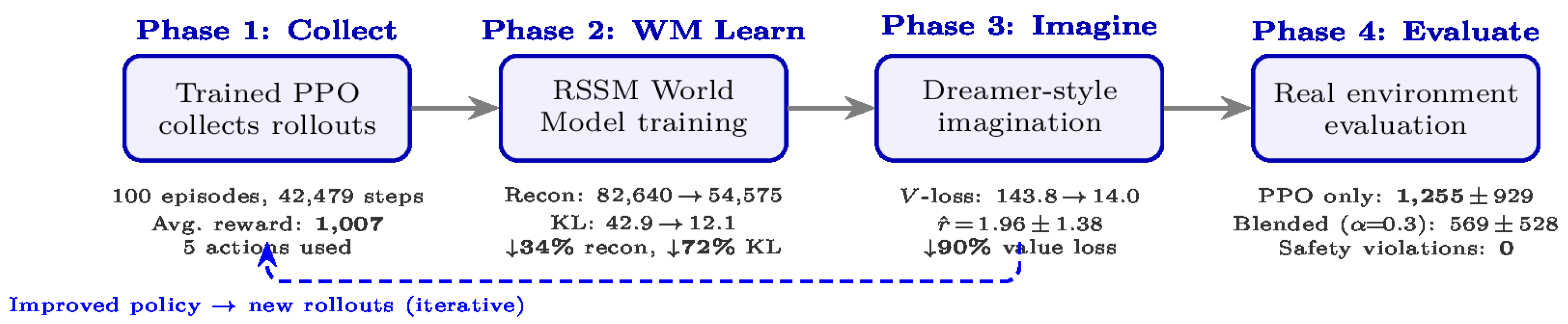
Figure 3.
Architecture of the health management system. Wearable sensor observations (IMU at three body sites and heart rate monitor) are encoded by the foundation encoder (Slot Attention + FM + FNO + DNC), and the RSSM world model learns physiological dynamics in a latent space for imagination-based policy optimization.
Figure 3.
Architecture of the health management system. Wearable sensor observations (IMU at three body sites and heart rate monitor) are encoded by the foundation encoder (Slot Attention + FM + FNO + DNC), and the RSSM world model learns physiological dynamics in a latent space for imagination-based policy optimization.
5.1. Domain Transfer via Encoder Replacement
The observation consists of IMU sensors at three body locations (36 dimensions) and heart-rate features (16 dimensions). The foundation encoder applies the same four-stage pipeline as MiniGrid, with modality-specific encoders replaced: Stage 1 treats IMU sites as slots and fuses them with heart rate via Cross-Attention; Stage 2 applies per-modality FM to each sensor group—without a pre-trained encoder, the FM must compensate for raw encoder noise; Stage 3 uses FNO fusion to encode the phase delay between physical movement and heart-rate response; Stage 4 provides episodic recall via DNC. The downstream pipeline (FM → FNO → DNC → PPO) is identical to MiniGrid, demonstrating the modularity claimed in Contribution 3.
5.2. Encoder Comparison
To validate that the foundation encoder improves policy quality beyond simpler encoders, we compare four variants sharing the same RSSM core, reward function, and PPO optimizer (Table 13).
The foundation encoder achieves 2.4× higher reward than the MLP baseline with 16× lower cross-seed variance ( vs. ), confirming that the per-modality FM stabilizes learning when no pre-trained encoder is available. The progression MLP → CNN → SlotAttn → Foundation shows that each additional layer of the proposed architecture contributes: structured attention (+28%), then FM+FNO+DNC (+47%). Safety violations decrease from 1.3 to 0.95 per episode.
This result, combined with the MiniGrid experiments where CLIP provides a strong pre-trained encoder and FM’s marginal effect is smaller, supports the central claim: the advantage of filter-before-mixing grows with encoder noise.
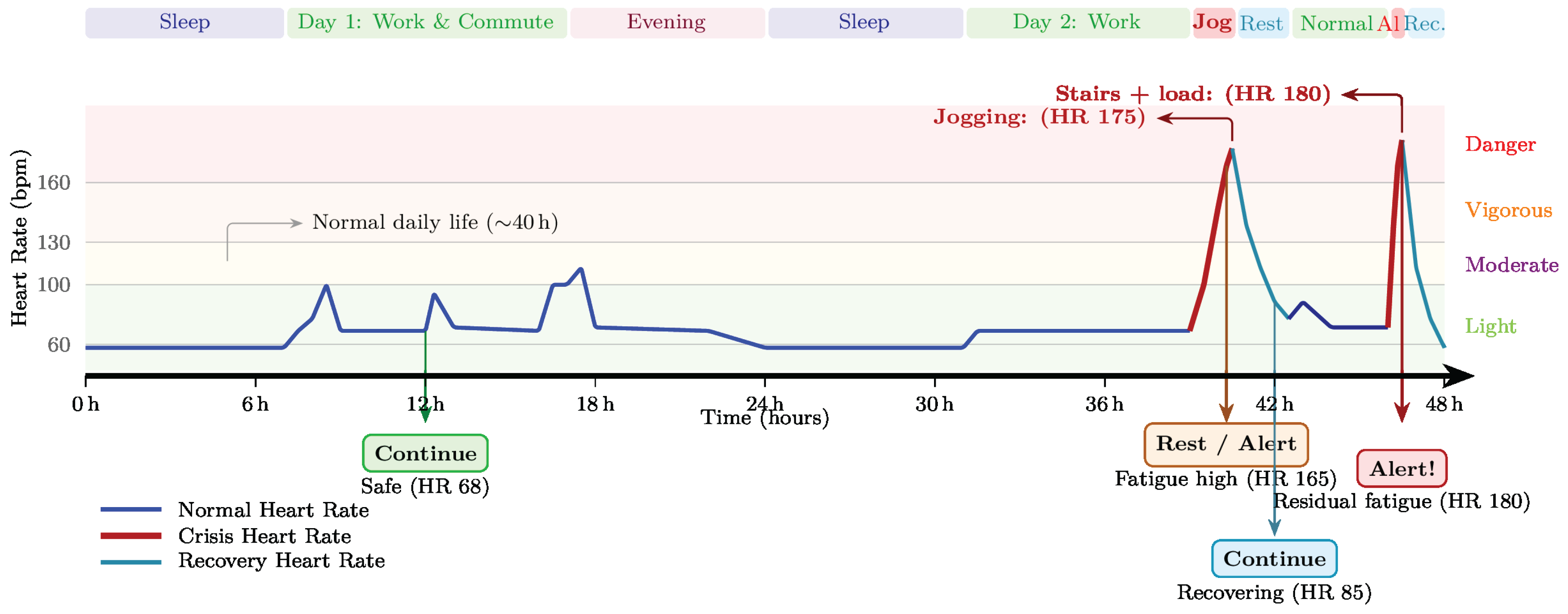
Figure 4.
Agent decision timeline over a 48-hour scenario. Top: life phases (sleep, commute, exercise, rest). Middle: heart rate with zone coloring (Light/Moderate/Vigorous/Danger). Bottom: agent decisions. Jogging raises HR to 175 bpm, triggering Rest/Alert. After recovery, stair-climbing with groceries raises HR to 180 bpm due to residual fatigue, triggering immediate Alert. KL spikes (↑KL) mark unexpected physiological changes.
Figure 4.
Agent decision timeline over a 48-hour scenario. Top: life phases (sleep, commute, exercise, rest). Middle: heart rate with zone coloring (Light/Moderate/Vigorous/Danger). Bottom: agent decisions. Jogging raises HR to 175 bpm, triggering Rest/Alert. After recovery, stair-climbing with groceries raises HR to 180 bpm due to residual fatigue, triggering immediate Alert. KL spikes (↑KL) mark unexpected physiological changes.
6. Discussion
6.1. Filter-Before-Mixing: When Does It Help?
The full architecture evaluation (Table 11) reveals a nuanced picture of when filter-before-mixing is beneficial. In MiniGrid with CLIP, the full architecture initially underperforms the Layer 1-only baseline (79% vs. 94% at 2000 episodes) because the additional FM/FNO/DNC parameters slow convergence. However, with continued training, the trajectories diverge dramatically: FreamerV1 reaches 87.7% ± 8.2% (one seed reaching 100%) while Layer 1 alone degrades to 78% due to catastrophic forgetting (Figure 2). This reveals a previously unrecognized role of per-modality FM: by enforcing modality-specific structure on the representations, FM acts as an implicit regularizer that prevents the policy from overfitting to recent experience and forgetting earlier knowledge.
In PAMAP2, where no pre-trained encoder exists and raw IMU/HR signals are noisy, the effect is immediate: the foundation encoder with FM achieves 2.4× higher reward and 16× lower variance than a vanilla MLP (Table 13). The central finding is therefore twofold: filter-before-mixing improves final performance in all settings through both representational enrichment and forgetting prevention, with the convergence cost largest when the encoder is already strong (MiniGrid + CLIP).
A noteworthy corollary is the dissociation between reconstruction accuracy and policy quality: the MLP encoder achieves the lowest reconstruction MSE (20.1) but the worst reward (113.6), while the foundation encoder shows the opposite. This suggests that per-modality FM optimizes representations for decision-making rather than reconstruction—consistent with the information-theoretic argument of Section 3.3.
6.2. The Role of Each Architectural Layer
The ablation and cross-domain results illuminate the relative contribution of each layer. At Layer 1, the frozen CLIP encoder accounts for +19.8 pp (Table 9), confirming that pre-trained visual representations are the most critical component in MiniGrid. In PAMAP2, Slot Attention + Cross-Attention alone improves reward from 113.6 (MLP) to 182.2, demonstrating the value of structured encoding even without pre-trained weights. At Layer 2, adding FM + FNO + DNC to SlotAttn+CrossAttn improves PAMAP2 reward from 182.2 to 268.3 (+47%), with the residual gate ensuring stable training by defaulting to identity until the velocity field is sufficiently trained. At Layer 3, the FNO’s contribution in MiniGrid is modest because modalities lack strong temporal delays, but in PAMAP2, where IMU activity precedes HR elevation by several seconds, the FNO’s phase-shift capability contributes to the 16× variance reduction. At Layer 4, the DNC’s contribution in MiniGrid is limited (rooms are visited sequentially), but in PAMAP2, episodic recall enables the agent to reference past physiological patterns across activity transitions.1
6.3. Computational Efficiency
The framework requires only 0.37M trainable parameters. The frozen CLIP encoder (92.6M) accounts for 99.6% of the total count but requires no gradient computation, and Score-based adaptive complexity estimation dynamically adjusts FM inference steps per state.
7. Conclusion
This paper proposed a design principle for multimodal reinforcement learning—filter before mixing—in which each modality’s representation is denoised by a dedicated Flow Matching module before cross-modal fusion via a Fourier Neural Operator in the spectral domain. This principle addresses the problem of cross-modal noise contamination that arises when heterogeneous modalities with different noise profiles are fused in a shared backbone, as is standard practice in monolithic VLA architectures such as 0.
We instantiated this principle in FreamerV1, a four-layer modular architecture integrating a frozen CLIP encoder with Slot Attention, per-modality Flow Matching, FNO spectral guidance, DNC episodic memory, and LLM-based language reward shaping. The framework achieves competitive performance with 0.37M trainable parameters—two orders of magnitude smaller than 0’s 3B—by exploiting the modular structure to freeze pre-trained components and train only the integration layers.
Experiments in three domains validated the approach. On MiniGrid navigation tasks, the full architecture (FM + FNO + DNC) reached 100% success on MultiRoom-N2-S4 at 5000 episodes, surpassing the 94% ceiling of the Layer 1-only baseline, though at the cost of slower initial convergence. On Crafter, an open-world environment without language instructions, the agent slightly surpassed DreamerV3’s official score (16.0% vs. 14.5%; single seed) using only three of four modality lines, demonstrating graceful degradation with missing modalities. On the PAMAP2 wearable-sensor health management task, the foundation encoder with per-modality Flow Matching, FNO fusion, and DNC memory achieved 2.4× higher cumulative reward ( vs. ), 27% fewer safety violations, and 16× lower cross-seed variance compared to a vanilla MLP-based RSSM world model. The dissociation between reconstruction accuracy and policy quality—the MLP encoder reconstructs observations better but produces worse policies—provides empirical support for the information-theoretic argument that pre-fusion denoising preserves policy-relevant information.
The health management application demonstrates that world model-based RL, which has seen remarkable success in games and robotics, can be extended to wearable-sensor health intervention with minimal architectural modification. The RSSM world model enables imagination-based policy optimization in the latent space, avoiding the ethical and practical difficulties of exposing real patients to dangerous physiological states during training. KL-divergence-based anomaly detection provides an additional safety layer for real-time physiological monitoring.
Several directions remain for future work. First, controlled comparisons against DreamerV3 on MiniGrid under identical conditions would further strengthen the experimental claims; preliminary results with the NM512 PyTorch reimplementation are ongoing. Second, extension to continuous-control robotic tasks and 3D environments would test the generality of the filter-before-mixing principle beyond discrete action spaces. Third, clinical validation of the health management application with domain experts and real patient outcomes is essential before deployment. Finally, the modest contribution of the FNO and DNC components in MiniGrid—where temporal delays between modalities are limited—motivates evaluation in domains with richer cross-modal dynamics, where the phase-shift capabilities of spectral-domain fusion are expected to be more fully realized. A direct experimental comparison of pre-fusion vs. post-fusion denoising (e.g., applying FM after FNO fusion rather than before) would further strengthen the information-theoretic argument for the filter-before-mixing principle.
7.1. Limitations
We acknowledge several limitations. For MiniGrid baselines, we conducted a controlled comparison against IMPALA under identical conditions, confirming the substantial performance gap (Table 10), but the PPO comparison relies on SB3 Zoo reference values [32] rather than identical conditions, and a controlled comparison against DreamerV3 remains for future work.
Regarding environment scope, MiniGrid is a 2D grid-world with discrete observations, and transfer to 3D environments, continuous-control tasks, and real robotic systems is unvalidated.
The ablation study removes one component at a time, so pairwise interaction effects (e.g., whether FM helps more or less when DNC is present) are not characterized.
For statistical reporting, the initial MiniGrid experiments (Table 7, Table 8 and Table 9) and the full architecture evaluation (Table 11) report single-seed results; multi-seed evaluation is ongoing. The IMPALA comparison uses 3 seeds with standard deviations, and the PAMAP2 encoder comparison (Table 13) uses 3 seeds.
The health management demonstration uses simulated rewards based on physiological heuristics, and clinical validation with domain experts is essential before deployment.
Finally, the FNO guidance layer and DNC memory show modest contributions in MiniGrid (Table 9), where the environment lacks strong temporal delays and long-horizon dependencies; their full potential is hypothesized to emerge in more complex domains, which remains to be validated.
Appendix A LLM-Based Mission Parser
Appendix A.1. Architecture and Caching
We employ Qwen2.5-3B-Instruct [24] as the mission parser. Given a mission string m, the model receives structured prompts and produces a JSON response from which four elements are extracted:
where is the final goal, are intermediate goals, is the action sequence, and are mentioned objects.
An LRU cache (capacity 1,000, keyed by MD5 hash) avoids redundant inference for identical missions, achieving >99% cache hit rates in practice. When LLM inference fails, a regex-based fallback parser ensures robustness:
Appendix A.2. Integration into Reward Computation
Parsing results drive the language-based reward:
where is the semantic match between parsed goals and the current state, is a goal-reached bonus, and is a proximity bonus.
Appendix A.3. Parsing Accuracy
Table A1 compares parsing accuracy across mission formats. The LLM parser substantially outperforms the regex baseline, particularly for compound instructions (+25 pp), novel expressions (+48 pp), and multilingual inputs (+94 pp).
Table A1.
Mission Parsing Accuracy
| Mission Format | Regex | Qwen-1.5B | Qwen-3B |
|---|---|---|---|
| Simple instructions | 95% | 98% | 99% |
| Compound instructions | 72% | 94% | 97% |
| Novel expressions | 45% | 89% | 93% |
| Multilingual | 0% | 91% | 94% |
| Average | 53% | 93% | 96% |
Appendix A.4. Effect on RL Performance
The parsing accuracy advantage translates to measurable improvements in downstream RL performance. Table A2 compares success rates at episode 2000 across the three parsers. The LLM parser yields higher success rates in both environments, with the improvement more pronounced in the complex N4-S5 environment (+6.2 pp for Qwen-3B over Regex), where compound missions require accurate decomposition into sub-goals.
Table A2.
Effect of Parser on RL Performance (Episode 2000)
| Environment | Parser | Success Rate | Avg. Steps |
|---|---|---|---|
| N2-S4 | Regex | 68.0% | 45.2 |
| Qwen2.5-1.5B | 70.5% | 42.8 | |
| Qwen2.5-3B | 71.2% | 41.5 | |
| N4-S5 | Regex | 42.3% | 78.5 |
| Qwen2.5-1.5B | 46.8% | 73.2 | |
| Qwen2.5-3B | 48.5% | 71.8 |
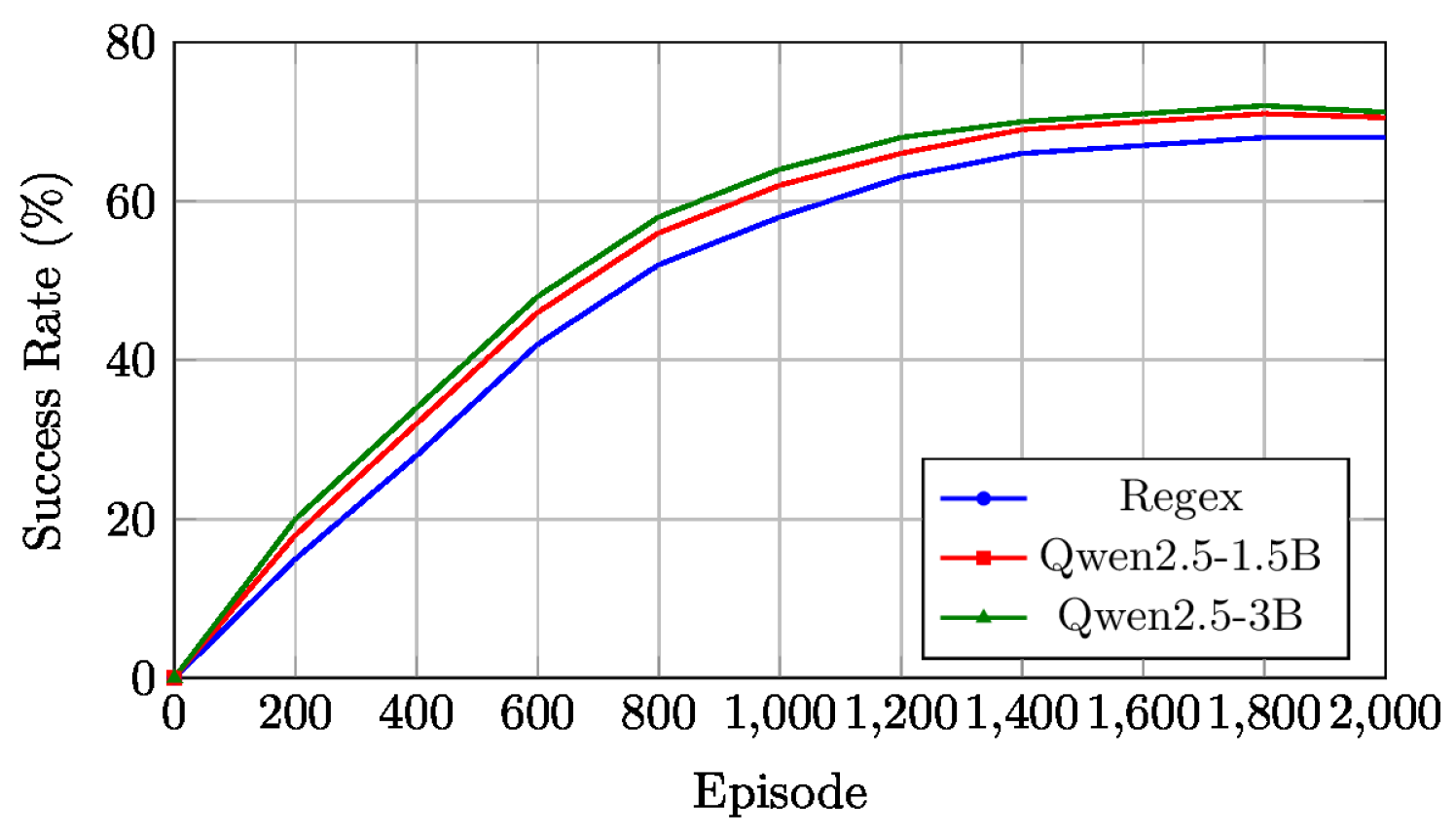
Figure A1 shows the learning curves for the MultiRoom-N2-S4 environment with the three parser configurations. The LLM-based parsers (Qwen2.5-1.5B and 3B) achieve faster initial learning and higher asymptotic performance than the regex baseline, confirming that accurate mission parsing provides more effective dense reward signals from the early stages of training. The Qwen-3B model shows a slight advantage over Qwen-1.5B, consistent with its higher parsing accuracy (Table A1).
Figure A1.
Learning curves for MultiRoom-N2-S4 with different mission parsers. The LLM-based parsers achieve faster convergence and higher asymptotic success rates than the regex baseline.
Figure A1.
Learning curves for MultiRoom-N2-S4 with different mission parsers. The LLM-based parsers achieve faster convergence and higher asymptotic success rates than the regex baseline.
Appendix A.5. Effect of Time Penalty
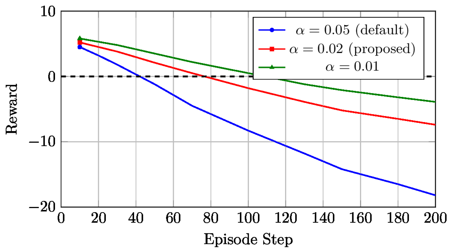
The language reward system includes a time penalty that discourages excessively long episodes, where is a scale parameter, is the current success rate, and t is the elapsed steps. Figure A2 illustrates the effect of the time penalty coefficient on the reward distribution.
With the default setting , a successful episode completing at step 145 can receive a reward as low as due to the accumulated time penalty, creating a misleading signal where successful behavior is penalized. Reducing to 0.02 alleviates this issue, yielding a reward distribution in which successful episodes receive consistently positive rewards while still discouraging unnecessarily long trajectories.
Figure A2.
Effect of time penalty coefficient on reward distribution. Reducing from 0.05 to 0.02 prevents successful episodes from receiving negative total rewards due to excessive time penalties.
Figure A2.
Effect of time penalty coefficient on reward distribution. Reducing from 0.05 to 0.02 prevents successful episodes from receiving negative total rewards due to excessive time penalties.
Appendix A.6. Computational Cost
Table A3 shows that the LRU cache reduces effective LLM inference time to <1 ms, limiting the total training time overhead to approximately 10%.
Table A3.
Computational Cost of Mission Parsing
| Method | Inference | Memory | Cache Hit | Total Time |
|---|---|---|---|---|
| (ms/ep) | (GB) | Rate | (h/2000ep) | |
| Regex | 0.1 | 0.1 | — | 2.5 |
| Qwen-1.5B | 35.2 (0.3*) | 2.1 | 99.2% | 2.8 |
| Qwen-3B | 52.8 (0.5*) | 4.2 | 99.1% | 3.1 |
| *Effective time on cache hit. | ||||
Appendix A.7. Parsing Examples and Failure Cases
Table A4 shows representative parsing outputs. The LLM parser correctly extracts goals and actions from compound instructions with nested sub-goals.
Table A4.
Parsing Examples
| Mission | Final Goal / Interm. | Actions |
|---|---|---|
| “traverse the rooms to get to the goal” | goal / [room] | [traverse, get] |
| “pick up the blue key and open the blue door” | door / [key] | [pick, open] |
| “find the yellow key then unlock the door to reach the goal” | goal / [key, door] | [find, unlock, reach] |
The following failure cases were observed: (1) extremely long mission descriptions (>100 words), (2) ambiguous instructions (e.g., “do something interesting”), and (3) references to concepts absent from the environment (e.g., “fly to the ceiling”). In all cases, the regex fallback maintains system stability.
Appendix B Hyperparameter Details
Table A5 lists the complete set of hyperparameters used across all experiments.
Table A5.
Complete Hyperparameter List
| Category | Parameter | Value |
|---|---|---|
| Architecture | CLIP model | ViT-B/32 |
| Slot dimension d | 128 | |
| Number of slots K | 8 | |
| RSSM dimension | 256 | |
| RSSM dimension | 64 | |
| DNC memory slots N | 32 | |
| DNC memory width W | 64 | |
| Flow Matching | Euler steps N | 4 |
| Velocity MLP hidden dim | 128 | |
| Gate init | ||
| FNO | Fourier modes K | 16 |
| Residual scale init | 0.1 | |
| Training | Optimizer | Adam |
| Learning rate | ||
| Adam | ||
| Gradient clip norm | 1.0 | |
| PPO clip | 0.2 | |
| PPO epochs per update | 4 | |
| GAE | 0.95 | |
| Discount | 0.99 | |
| Reward | 0.2 | |
| 0.1 | ||
| 0.2 | ||
| (WM) | 0.1 | |
| World Model | (KL weight) | 0.5 |
| Free nats | 1.0 |
Appendix C PAMAP2 Dataset Details
The PAMAP2 dataset [37] contains data from 9 subjects performing 18 physical activities, recorded with 3 IMU sensors (hand, chest, ankle) and a heart rate monitor. Each IMU provides 3-axis accelerometer, gyroscope, and magnetometer readings (12 dimensions per site, 36 total). The heart-rate-related features (16 dimensions) comprise the raw heart rate, activity one-hot encoding (8 categories), and derived features: heart rate zone (Light/Moderate/Vigorous/Danger), fatigue estimate (exponential moving average of exertion), heart rate variability, rate of change, and cumulative exertion.
The health management reward function is a weighted combination of three components:
where penalizes heart rates outside safe zones, rewards maintaining the target heart rate for the current activity, and penalizes accumulated fatigue. The discrete action space consists of: Continue (maintain current activity), Rest (reduce intensity), Increase (raise intensity), Change (switch activity type), and Alert (emergency stop).
Appendix D Flow Matching and FNO Mathematical Details
Appendix D.1. Conditional Flow Matching Formulation
The flow is defined by the ODE:
The CFM training loss for modality m is:
Appendix D.2. FNO Spectral Convolution
The spectral convolution applies FFT, complex multiplication by learnable weights , and IFFT:
with smoothness regularization:
Appendix D.3. Phase-Shift Representation
The cross-correlation delay between modalities appears as:
Appendix D.4. Approximation Bound
The pre-fusion mutual information bound:
See Appendix J for the full derivation.
Appendix E Layer 1 Encoder Details
Appendix E.1. Vision Encoder
The frozen CLIP ViT-B/32 [11] produces patch features , projected via . Slot Attention [12] decomposes these into K slots through iterative competitive assignment:
Numerical stabilization techniques: (1) Mask values use instead of . (2) NaN fallback substitutes uniform . (3) GRU weights: Xavier (gain 0.5) + Orthogonal (gain 0.5). (4) Variance clipping: .
Appendix E.2. Language, State, and Reward Encoders
Language: A Transformer encoder [21] produces . Slot Attention [12] is applied to decompose mission components.
State: FNO block [16] with spectral convolution .
Reward: .
Appendix E.3. Cross-Modal Attention
Appendix F Layer 4 Details
Appendix F.1. DNC Memory
The DNC [17] uses content-based addressing: . Write: . Read: . Output: .
Appendix F.2. PPO Objective
Appendix G Auxiliary Component Details
Appendix G.1. Language-Grounded Reward
Appendix G.2. Adaptive Reward Shaping
Following the potential-based reward shaping framework [26]: , where is the recent success rate.
Appendix G.3. Success Buffer
Inspired by Hindsight Experience Replay [27], successful episodes are stored and replayed at 25% mix ratio during training to prevent catastrophic forgetting.
Appendix G.4. Score-Based Adaptive Complexity
Appendix H RSSM Limitations and Input-Side Design
Appendix H.1. Addressing RSSM Limitations via Input-Side Design
The standard RSSM architecture [1] processes observations through a single encoder before the deterministic–stochastic state transition, which introduces three structural limitations for multimodal sensor-driven applications. First, a single encoder conflates modalities with fundamentally different noise profiles (e.g., sparse reward signals and high-frequency IMU readings), losing modality-specific structure. Second, the GRU-based deterministic pathway provides only short-term memory, insufficient for recalling episodic patterns such as prior heart-rate spikes across activity transitions. Third, standard real-valued fusion (concatenation or attention) cannot represent phase-shifted cross-modal correlations, such as the several-second delay between physical movement (IMU) and heart-rate elevation.
Our approach addresses these limitations not by modifying the RSSM’s internal dynamics, but by improving the quality of the observation representation that enters the RSSM posterior. Per-modality Flow Matching preserves modality-specific noise characteristics by denoising each signal independently before fusion. FNO spectral fusion encodes phase-shifted correlations through learnable complex-valued spectral weights (Eq. (A10)). DNC external memory supplements the GRU’s short-term state with content-addressable episodic recall. This input-side design is complementary to approaches that modify the RSSM itself, such as MedDreamer’s Adaptive Feature Integration module [8] for irregular clinical time series, and could in principle be combined with such internal modifications.
Appendix I PAMAP2 World Model: Full Implementation Details
This appendix provides the complete implementation details of the PAMAP2 health management application described in Section 5. The system uses a Recurrent State-Space Model (RSSM) as the world model backbone, with the proposed foundation encoder (Slot Attention + per-modality FM + FNO + DNC) as the observation encoder. The agent learns to recommend health interventions (Continue, Adjust Intensity, Rest, Alert) by imagining future physiological trajectories in the latent space, avoiding the ethical and practical difficulties of exposing real subjects to dangerous physiological states during training.
Appendix I.1. RSSM World Model Architecture
The world model follows the RSSM of DreamerV3 [1], representing the latent state as the concatenation of a deterministic component (256 dimensions) and a stochastic component (64 dimensions), yielding a 320-dimensional state vector (Figure A3).
Figure A3.
RSSM world model for PAMAP2 health management. Top: temporal unrolling showing the deterministic pathway (GRU transitions) and stochastic pathway (prior/posterior distributions). Bottom: four-phase training pipeline with experimental results.
Figure A3.
RSSM world model for PAMAP2 health management. Top: temporal unrolling showing the deterministic pathway (GRU transitions) and stochastic pathway (prior/posterior distributions). Bottom: four-phase training pipeline with experimental results.
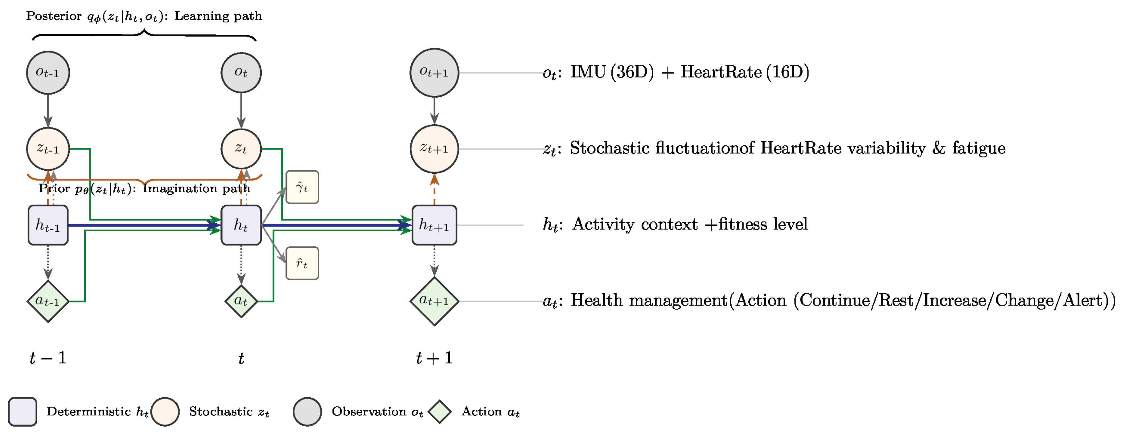
The deterministic pathway retains temporal context of activity patterns through a GRU:
The stochastic pathway models uncertainty through prior and posterior distributions:
where is the output of the foundation encoder (Section 5). The posterior conditions on observations via the encoder, while the prior enables imagination without observations.
Appendix I.2. Foundation Encoder Details
The observation consists of IMU sensors at three body locations (accelerometer, gyroscope, magnetometer; 36 dimensions) and heart-rate-related features (16 dimensions). The foundation encoder applies the four-stage pipeline:
Stage 1 (Slot Attention): The three IMU sites ( dimensions) are treated as slots and processed by Self-Attention, then fused with heart rate features via Cross-Attention:
Stage 2 (Per-Modality Flow Matching): Independent FM modules refine the IMU and HR representations before fusion. Without a pre-trained encoder (no CLIP equivalent for IMU data), the FM refinement compensates for the raw encoder’s noise—this is the setting where filter-before-mixing is most critical.
Stage 3 (FNO Spectral Fusion): The refined modality representations are fused via SpectralConv1d. The phase-shift property of the FNO (Eq. (A10)) is particularly relevant here, as physical movement (IMU) precedes heart rate elevation by several seconds.
Stage 4 (DNC Memory): The fused representation is augmented with episodic memory via content-based addressing [17], enabling the agent to recall past physiological episodes (e.g., a prior heart-rate spike that triggered a rest recommendation).
The final encoded observation enters the RSSM posterior (Eq. (A18)).
Appendix I.3. World Model Training
The world model is trained by minimizing:
where reconstructs observations (MSE on IMU + HR features), predicts rewards (health outcomes), predicts episode continuation (activity transitions), and balances KL regularization.
Appendix I.4. Imagination-Based Policy Optimization
Using only the prior distribution, imagined rollouts of horizon are generated to optimize the policy without real-world interaction:
The policy and value function are updated via -returns computed over imagined trajectories.
The reward function combines physiological targets (heart rate within safe range, activity level maintenance, fatigue prevention) with safety constraints (penalizing prolonged exposure to dangerous heart rate zones >160 bpm). This imagination-based training is particularly valuable for health management: learning appropriate Alert actions requires repeated exposure to high-risk states, which is ethically and practically infeasible in real patients. The world model generates such scenarios safely in the latent space.
Appendix I.5. Physiological Anomaly Detection
As a byproduct of the world model, the KL divergence at each time step quantifies how much the actual sensor observation deviates from the world model’s prediction. Time steps where (where and are the running mean and standard deviation of KL values) are flagged as anomaly candidates, indicating unexpected heart rate elevation or atypical fatigue patterns. This mechanism provides an additional safety layer not present in MedDreamer or KANDI (Table A6).
Appendix I.6. Positioning Among Health Intervention Systems
Table A6 compares our approach with recent world model-based health intervention systems. Direct numerical comparison is not meaningful across different clinical domains; the table highlights architectural differences.
Table A6.
Comparison with World Model-Based Health Intervention Systems
| MedDreamer [8] | KANDI [9] | DreamerV3 [1] | FreamerV1 (ours) | |
|---|---|---|---|---|
| Domain | EHR (Sepsis) | Wearable (fall risk) | General RL | Wearable (health) |
| World model | RSSM+AFI | None | RSSM | RSSM+Foundation |
| Policy | Actor-Critic | Diffusion | Actor-Critic | PPO |
| Learning | Online+Imag. | Offline IRL | Online+Imag. | Online+Imag. |
| Encoding | AFI | MLP | CNN/MLP | SlotAttn+FM+FNO |
| Anomaly | — | — | — | KL divergence |
Our system shares with MedDreamer the paradigm of RSSM-based imagination for safe policy learning, but addresses a different data regime: continuous, high-frequency, multi-site wearable signals rather than sparse, irregular EHR records. Compared to KANDI, our approach learns an explicit world model and optimizes policies through imagination, whereas KANDI operates offline with pre-collected expert demonstrations.
Appendix I.7. Generalization Across Subjects
After pre-training the world model on data from multiple subjects, the policy can be adapted to new subjects with minimal data. While inter-subject variability exists in resting heart rate and cardiopulmonary capacity, higher-level decision structures—such as recommending rest under high exertion or alerting upon fatigue accumulation—are shared in the latent space of the world model, enabling few-shot adaptation.
Appendix J Derivation of the Approximation Bound
We derive the bound stated in Eq. (A11). Let denote the clean representation of modality m, the noisy encoding with , and the FM-denoised representation with error .
The mutual information between the clean signals and the pre-fusion representation can be written as:
When the fusion function f is Lipschitz continuous with constant (satisfied by the FNO with bounded spectral weights), a second-order Taylor expansion around yields:
The first term equals evaluated at the Bayes-optimal denoised representations. Since measures how far the per-modality FM is from optimal denoising, the bound shows that pre-fusion denoising is beneficial whenever is small—i.e., when the FM denoising error is smaller than the original noise, a substantially weaker condition than perfect denoising.
With the residual gate , the effective error becomes , and the bound tightens to:
Since when the FM velocity field is untrained, the penalty vanishes at initialization, ensuring that the pre-fusion approach is never worse than no denoising during the early stages of training.
References
- Hafner, D.; Pasukonis, J.; Ba, J.; Lillicrap, T. Mastering Diverse Domains through World Models. Proc. Proc. 40th Int. Conf. Mach. Learn. (ICML) 2023, Vol. 202, 12385–12410. [Google Scholar]
- Black, K.; Brown, N.; Driess, D.; Esmail, A.; Equi, M.; Finn, C.; Fusai, N.; Groom, L.; Hausman, K.; Ichter, B.; et al. π0: A Vision-Language-Action Flow Model for General Robot Control. In Proceedings of the Proc. Robotics: Science and Systems (RSS), 2025. [Google Scholar]
- Bruce, J.; Dennis, M.; Edwards, A.; Parker-Holder, J.; Shi, Y.; Hughes, E.; Lai, M.; Mavalankar, A.; Steiber, R.; Apps, C.; et al. Genie 2: A Large-Scale Foundation World Model. Google Deep. Blog 2024. [Google Scholar]
- Alonso, E.; Jelley, A.; Sherwin, V.; Kanervisto, A.; Sherr, T. Diffusion for World Modeling: Visual Details Matter in Atari. In Proceedings of the Proc. NeurIPS, 2024. [Google Scholar]
- Krohn, R.; Prasad, V.; Tiboni, G.; Chalvatzaki, G. Self-Supervised Multisensory Pretraining for Contact-Rich Robot Reinforcement Learning. IEEE Robotics and Automation Letters (RA-L), 2025. [Google Scholar]
- Liu, Q.; Cui, Y.; Sun, Z.; Li, G.; Chen, J.; Ye, Q. VTDexManip: A Dataset and Benchmark for Visual-Tactile Pretraining and Dexterous Manipulation with Reinforcement Learning. In Proceedings of the Proc. ICLR, 2025. [Google Scholar]
- Meng, H.; Guo, X.; Liu, P.; Feng, J.; Guo, D.; Liu, H. Multimodal Information Bottleneck for Deep Reinforcement Learning with Multiple Sensors. Neural Netw. 2024, 176, 106347. [Google Scholar]
- Xu, Q.; Habib, G.; Wu, F.; Perera, D.; Feng, M. medDreamer: Model-Based Reinforcement Learning with Latent Imagination on Complex EHRs for Clinical Decision Support. In Proceedings of the Proc. KDD, 2026. [Google Scholar]
- Liu, C.; Xie, R.; Park, J.H.; Stout, J.; Thiamwong, L. Diffusion Policies with Offline and Inverse Reinforcement Learning for Promoting Physical Activity in Older Adults Using Wearable Sensors. In Proceedings of the Proc. ICMLA, 2025. [Google Scholar]
- Reed, S.; Zolna, K.; Parisotto, E.; Colmenarejo, S.G.; Novikov, A.; Barth-Maron, G.; Gimenez, M.; Sulsky, Y.; Kay, J.; Springenberg, J.T.; et al. A Generalist Agent. In Trans. Mach. Learn. Res.; 2022. [Google Scholar]
- Radford, A.; Kim, J.W.; Hallacy, C.; Ramesh, A.; Goh, G.; Agarwal, S.; Sastry, G.; Askell, A.; Mishkin, P.; Clark, J.; et al. Learning Transferable Visual Models from Natural Language Supervision. In Proceedings of the Proc. ICML, 2021. [Google Scholar]
- Locatello, F.; Weissenborn, D.; Unterthiner, T.; Mahendran, A.; Heigold, G.; Uszkoreit, J.; Dosovitskiy, A.; Kipf, T. Object-Centric Learning with Slot Attention. In Proceedings of the Proc. NeurIPS, 2020. [Google Scholar]
- Kipf, T.; Elsayed, G.F.; Mahendran, A.; Stone, A.; Sabour, S.; Heigold, G.; Jonschkowski, R.; Dosovitskiy, A.; Greff, K. Conditional Object-Centric Learning from Video. In Proceedings of the Proc. ICLR, 2022. [Google Scholar]
- Ajay, A.; Du, Y.; Gupta, A.; Tenenbaum, J.B.; Jaakkola, T.; Agrawal, P. Is Conditional Generative Modeling All You Need for Decision-Making? In Proceedings of the Proc. ICLR, 2023. [Google Scholar]
- Chi, C.; Feng, S.; Du, Y.; Xu, Z.; Cousineau, E.; Burchfiel, B.; Song, S. Diffusion Policy: Visuomotor Policy Learning via Action Diffusion. In Proceedings of the Proc. RSS, 2023. [Google Scholar]
- Li, Z.; Kovachki, N.; Azizzadenesheli, K.; Liu, B.; Bhatt, K.; Stuart, A.; Anandkumar, A. Fourier Neural Operator for Parametric Partial Differential Equations. In Proceedings of the Proc. ICLR, 2021. [Google Scholar]
- Graves, A.; Wayne, G.; Reynolds, M.; Harley, T.; Danihelka, I.; Grabska-Barwińska, A.; Colmenarejo, S.G.; Grefenstette, E.; Ramalho, T.; Agapiou, J.; et al. Hybrid Computing Using a Neural Network with Dynamic External Memory. Nature 2016, 538, 471–476. [Google Scholar] [CrossRef] [PubMed]
- Wayne, G.; Hung, C.C.; Amos, D.; Mirza, M.; Ahuja, A.; Grabska-Barwińska, A.; Rae, J.; Mirowski, P.; Leibo, J.Z.; Santoro, A.; et al. Unsupervised Predictive Memory in a Goal-Directed Agent. arXiv 2018, arXiv:1803.10760. [Google Scholar] [CrossRef]
- Hafner, D.; Lillicrap, T.; Norouzi, M.; Ba, J. Mastering Atari with Discrete World Models. In Proceedings of the Proc. ICLR, 2021. [Google Scholar]
- Schrittwieser, J.; Antonoglou, I.; Hubert, T.; Simonyan, K.; Sifre, L.; Schmitt, S.; Guez, A.; Lockhart, E.; Hassabis, D.; Graepel, T.; et al. Mastering Atari, Go, Chess and Shogi by Planning with a Learned Model. Nature 2020, 588, 604–609. [Google Scholar] [CrossRef] [PubMed]
- Vaswani, A.; Shazeer, N.; Parmar, N.; Uszkoreit, J.; Jones, L.; Gomez, A.N.; Kaiser, Ł.; Polosukhin, I. Attention Is All You Need. In Proceedings of the Proc. NeurIPS, 2017. [Google Scholar]
- Lipman, Y.; Chen, R.T.Q.; Ben-Hamu, H.; Nickel, M.; Le, M. Flow Matching for Generative Modeling. In Proceedings of the Proc. ICLR, 2023. [Google Scholar]
- Schulman, J.; Wolski, F.; Dhariwal, P.; Radford, A.; Klimov, O. Proximal Policy Optimization Algorithms. arXiv 2017, arXiv:1707.06347. [Google Scholar] [CrossRef]
- Qwen Team. Qwen2.5: A Party of Foundation Models. arXiv 2024, arXiv:2412.15115. [Google Scholar]
- Cover, T.M.; Thomas, J.A. Elements of Information Theory, 2nd ed.; Wiley, 2006. [Google Scholar]
- Ng, A.Y.; Harada, D.; Russell, S. Policy Invariance under Reward Transformations: Theory and Application to Reward Shaping. In Proceedings of the Proc. ICML, 1999. [Google Scholar]
- Andrychowicz, M.; Wolski, F.; Ray, A.; Schneider, J.; Fong, R.; Welinder, P.; McGrew, B.; Tobin, J.; Abbeel, P.; Zaremba, W. Hindsight Experience Replay. In Proceedings of the Proc. NeurIPS, 2017. [Google Scholar]
- Song, Y.; Sohl-Dickstein, J.; Kingma, D.P.; Kumar, A.; Ermon, S.; Poole, B. Score-Based Generative Modeling through Stochastic Differential Equations. In Proceedings of the Proc. ICLR, 2021. [Google Scholar]
- Xu, J.; Mei, T.; Yao, T.; Rui, Y. MSR-VTT: A Large Video Description Dataset for Bridging Video and Language. In Proceedings of the Proc. CVPR, 2016. [Google Scholar]
- Chevalier-Boisvert, M.; Dai, B.; Towers, M.; de Lazcano, R.; Willems, L.; Lahlou, S.; Pal, S.; Castro, P.S.; Terry, J. Minigrid & Miniworld: Modular & Customizable Reinforcement Learning Environments. In Proceedings of the Proc. NeurIPS, 2023. [Google Scholar]
- Chevalier-Boisvert, M.; Bahdanau, D.; Lahlou, S.; Willems, L.; Saharia, C.; Nguyen, T.H.; Bengio, Y. BabyAI: A Platform to Study the Sample Efficiency of Grounded Language Learning. In Proceedings of the Proc. ICLR, 2019. [Google Scholar]
- Zoo, RL Baselines3. Pre-Trained RL Agents Using Stable-Baselines3. 2023. Available online: https://github.com/DLR-RM/rl-baselines3-zoo.
- Espeholt, L.; Soyer, H.; Munos, R.; Simonyan, K.; Mnih, V.; Ward, T.; Doron, Y.; Firoiu, V.; Harley, T.; Dunning, I.; et al. IMPALA: Scalable Distributed Deep-RL with Importance Weighted Actor-Learner Architectures. In Proceedings of the Proc. ICML, 2018. [Google Scholar]
- Ferrao, J.L.; Cunha, R.F. World Model Agents with Change-Based Intrinsic Motivation. Proc. Proc. North. Light. Deep Learn. Conf. (NLDL) 2025, Vol. 265. PMLR. [Google Scholar]
- Chen, L.; Lu, K.; Rajeswaran, A.; Lee, K.; Grover, A.; Laskin, M.; Abbeel, P.; Srinivas, A.; Mordatch, I. Decision Transformer: Reinforcement Learning via Sequence Modeling. In Proceedings of the Proc. NeurIPS, 2021. [Google Scholar]
- Hafner, D. Benchmarking the Spectrum of Agent Capabilities. In Proceedings of the Proc. ICLR, 2022. [Google Scholar]
- Reiss, A.; Stricker, D. Introducing a New Benchmarked Dataset for Activity Recognition. In Proceedings of the Proc. 16th Int. Symp. Wearable Computers (ISWC), 2012; pp. 108–109. [Google Scholar]
- Schulman, J.; Moritz, P.; Levine, S.; Jordan, M.; Abbeel, P. High-Dimensional Continuous Control Using Generalized Advantage Estimation. In Proceedings of the Proc. ICLR, 2016. [Google Scholar]
- Pathak, D.; Agrawal, P.; Efros, A.A.; Darrell, T. Curiosity-Driven Exploration by Self-Supervised Prediction. In Proceedings of the Proc. ICML, 2017. [Google Scholar]
- Jang, E.; Gu, S.; Poole, B. Categorical Reparameterization with Gumbel-Softmax. In Proceedings of the Proc. ICLR, 2017. [Google Scholar]
| 1 | A detailed analysis of how FreamerV1 addresses structural limitations of the standard RSSM (single-encoder conflation, short-term GRU memory, phase-shift representation) is provided in Appendix H. |
Figure 1.
Overall Architecture of the Proposed Method
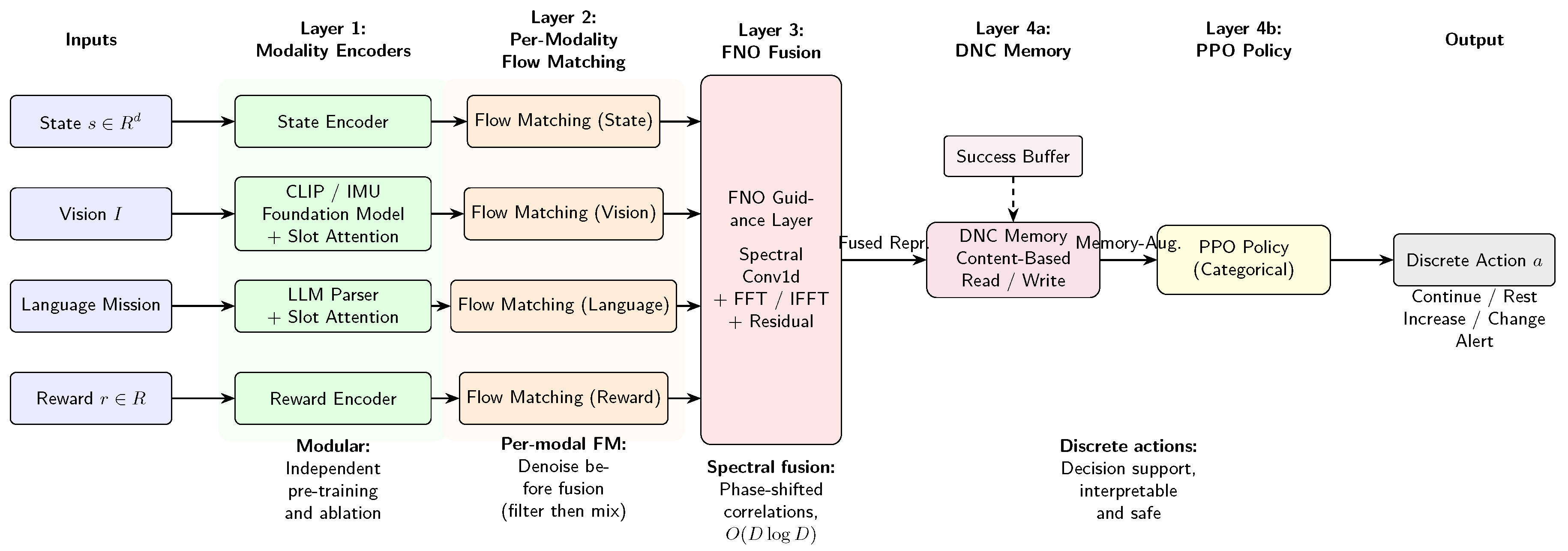
Figure 2.
Learning curves on MultiRoom-N2-S4 (5000 episodes). FreamerV1 (purple, 3 seeds with min–max band) shows steady improvement without forgetting, reaching 87.7% ± 8.2%. Layer 1 only (red) peaks early but degrades to 78% due to catastrophic forgetting. One seed (seed 2) reaches 100% at episode 4800.
Figure 2.
Learning curves on MultiRoom-N2-S4 (5000 episodes). FreamerV1 (purple, 3 seeds with min–max band) shows steady improvement without forgetting, reaching 87.7% ± 8.2%. Layer 1 only (red) peaks early but degrades to 78% due to catastrophic forgetting. One seed (seed 2) reaches 100% at episode 4800.
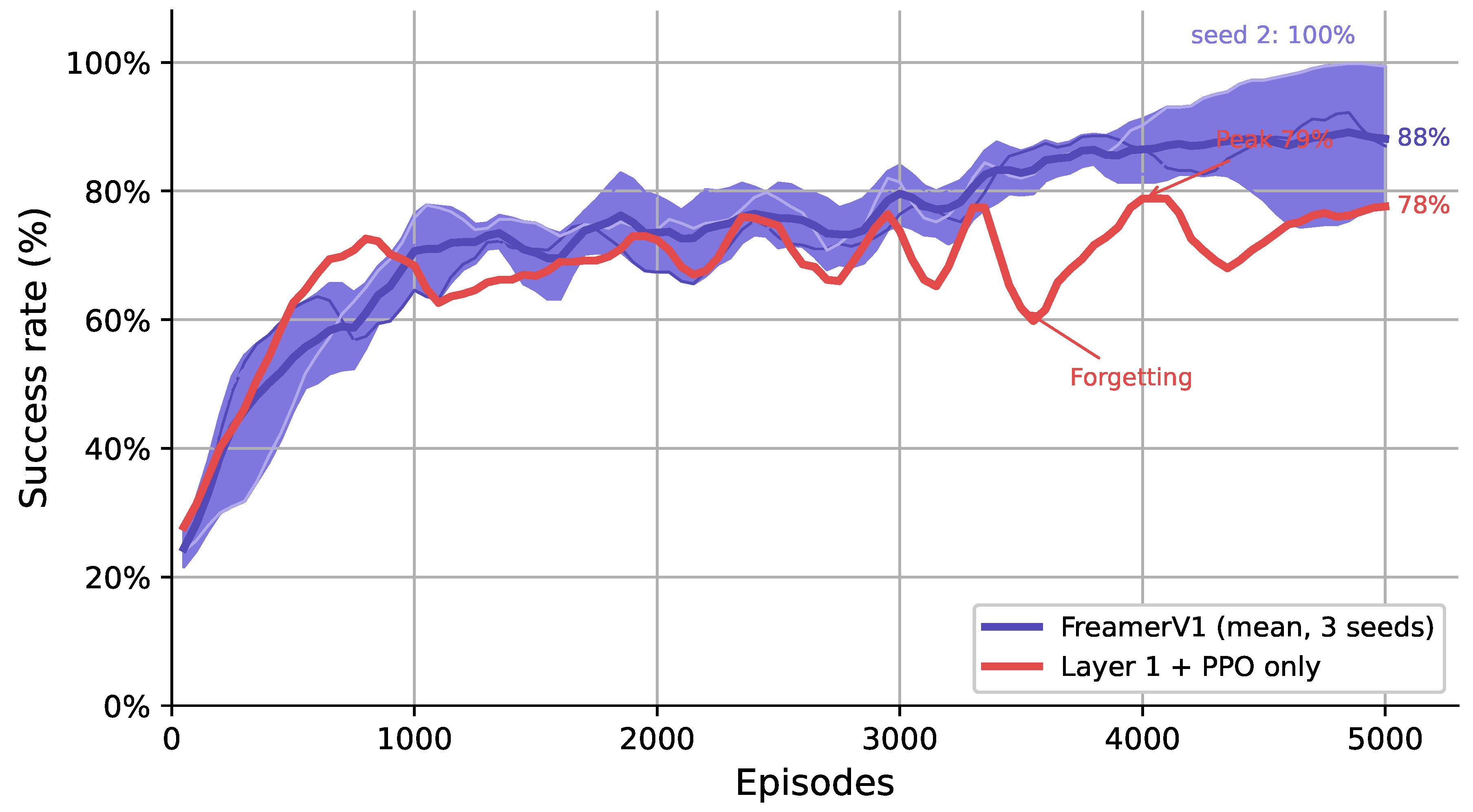
Table 1.
Design Differentiation from 0. The two systems target fundamentally different regimes: 0 addresses continuous-control robotic manipulation with large-scale demonstration data, while our framework targets discrete-action sensor-driven domains with limited data.
Table 1.
Design Differentiation from 0. The two systems target fundamentally different regimes: 0 addresses continuous-control robotic manipulation with large-scale demonstration data, while our framework targets discrete-action sensor-driven domains with limited data.
| Design Aspect | 0 | FreamerV1 (ours) |
|---|---|---|
| Target domain | Robotic manipulation | Sensor-driven decision |
| Architecture | Monolithic VLM | Modular per-modality |
| FM target | Actions (output) | Representations (internal) |
| Cross-modal fusion | Self-attention | FNO (spectral domain) |
| Action space | Continuous | Discrete |
| External memory | None | DNC |
| Parameters | 3B | 93M (0.4M trainable) |
Table 2.
Capability Comparison with Related Methods
| Method | Per-modal | Spectral | Language | External | Health | Scale | Cont. |
|---|---|---|---|---|---|---|---|
| Gen. Enc. | Fusion | Reward | Memory | WM | >1B | Ctrl | |
| DreamerV3 | – | – | – | – | – | – | ◯ |
| 0 | – | – | – | – | – | ◯ | ◯ |
| DIAMOND | – | – | – | – | – | – | – |
| Decision Diff. | – | – | – | – | – | – | ◯ |
| Diffusion Policy | – | – | – | – | – | – | ◯ |
| MERLIN | – | – | – | ◯ | – | – | ◯ |
| MedDreamer | – | – | – | – | ◯ | – | – |
| KANDI | – | – | – | – | ◯ | – | – |
| FreamerV1 (ours) | ◯ | ◯ | ◯ | ◯ | ◯ | – | – |
Per-modal Gen. Enc.: per-modality generative encoding (FM on representations). Spectral Fusion: FNO-based cross-modal fusion. Language Reward: LLM-based dense reward shaping. External Memory: DNC or equivalent. Health WM: world model applied to health intervention. Scale >1B: model with >1B parameters. Cont. Ctrl: validated on continuous-control tasks.
Table 3.
Model Configuration
| Parameter | Value |
|---|---|
| Visual Encoder | CLIP ViT-B/32 (frozen) |
| Vision/Language Slots | 8 |
| Slot Dimension | 128 |
| Flow Matching Steps | 4 |
| FNO Fourier Modes | 16 |
| DNC Memory Slots | 32 |
| PPO Clip | 0.2 |
| Learning Rate | |
| Gradient Clip Norm | 1.0 |
Table 4.
Parameter Count
| Component | Parameters |
|---|---|
| CLIP Visual Encoder (frozen) | 92.68M |
| Slot Attention + Cross-Modal Attn | 0.08M |
| Flow Matching ( modalities) | 0.06M |
| FNO Guidance Layer | 0.02M |
| DNC Memory | 0.04M |
| Policy + Value Heads | 0.17M |
| Total | 93.05M |
| Trainable | 0.37M (0.4%) |
Table 6.
Cross-Modal Alignment Loss (MSR-VTT)
| Encoder | Alignment Loss |
|---|---|
| CNN + Average Pooling | 2.34 |
| CNN + Slot Attention | 1.87 |
| CLIP + Average Pooling | 1.52 |
| CLIP + Slot Attention (Proposed) | 1.21 |
Table 7.
MiniGrid Results
| Environment | Episodes | Success Rate | Best Reward |
|---|---|---|---|
| DoorKey | |||
| DoorKey-5x5 | 1,789 | — | 0.975 |
| DoorKey-8x8 | 3,738 | 20.0% | 6.294 |
| MultiRoom | |||
| N2-S4 | 1,090 | 94.0% | 0.932 |
| N2-S5 | 592 | 35.0% | 0.946 |
| N3-S4‡ | 673 | 46.0% | 0.921 |
| N3-S5‡ | 1,996 | 59.0% | 0.937 |
| N4-S4‡ | 1,103 | 93.0% | 0.917 |
| N4-S5‡ | 27 | 35.7% | 0.904 |
| N4-S5 (from scratch) | 2,000 | 0.0% | — |
| ‡Curriculum learning: initialized from a simpler environment’s checkpoint. | |||
Table 8.
Comparison with Standard PPO (SB3 Zoo Reference Values)
| Environment | PPO† | Proposed | Improvement |
|---|---|---|---|
| MultiRoom-N2-S4 | 65% | 94.0% | +44.6 pp |
| MultiRoom-N3-S4 | 35% | 46.0% | +31.4 pp |
| † Reference values from SB3 Zoo [32] (FlatObsWrapper). | |||
Table 9.
Ablation Study (MultiRoom-N2-S5)
| Configuration | Success Rate | Δ |
|---|---|---|
| Full (Proposed) | 35.0% | — |
| − CLIP (using CNN encoder) | 15.2% | −19.8 pp |
| − Adaptive Reward Shaping | 27.0% | −8.0 pp |
| − Success Buffer | 31.0% | −4.0 pp |
| SAC instead of PPO | 0.1% | −34.9 pp |
Table 10.
Literature-Based Positioning on MiniGrid
| Method | Type | MiniGrid Finding | Ref. |
|---|---|---|---|
| PPO (SB3) | MF | N2-S4: 65%*, N3-S4: 35%* | [32] |
| IMPALA‡ | MF | N2-S4: 43%, N4-S5: 0%, N6: 0% | [33] |
| DreamerV3 | MB | Suboptimal convergence on MiniGrid | [34] |
| Dec. Trans. | Offline | Key-to-Door: 94%; requires demos | [35] |
| FreamerV1 (ours) | MF | N2-S4: 94%, N4-S4: 93% | — |
| *Reference values. ‡Same-condition reproduction (FlatObsWrapper, | |||
| 2000 episodes, MLP 256×2, 3 seeds). MF: model-free, MB: model-based. | |||
Table 11.
Full Architecture Evaluation (MultiRoom-N2-S4). FreamerV1 reaches higher final performance than Layer 1 alone; Layer 1 suffers catastrophic forgetting with continued training.
Table 11.
Full Architecture Evaluation (MultiRoom-N2-S4). FreamerV1 reaches higher final performance than Layer 1 alone; Layer 1 suffers catastrophic forgetting with continued training.
| Configuration | 2000 ep | 5000 ep | Seeds |
|---|---|---|---|
| FreamerV1 (ours) | 79.0% | 87.7% ± 8.2% | 3 |
| − DNC (FM + FNO only) | 80.0% | — | 1 |
| Layer 1 + PPO only | 94.0% | 78.0% | 1 |
Table 12.
Crafter Results ( steps, single seed). Score: official Crafter metric [36]. Avg Ep Ach: mean achievements per episode. Ach: unique types unlocked during training.
Table 12.
Crafter Results ( steps, single seed). Score: official Crafter metric [36]. Avg Ep Ach: mean achievements per episode. Ach: unique types unlocked during training.
| Method | Score | Avg Ep Ach | Ach |
|---|---|---|---|
| Human expert | 50.5% | — | — |
| DreamerV3 | 14.5% | — | — |
| PPO | 4.6% | — | — |
| FreamerV1 (ours, w/ shaping) | 16.0% | 4.5 | 16/22 |
| FreamerV1 (ours, w/o shaping) | 14.9% | — | 17/22 |
| No language modality available in Crafter. | |||
Table 13.
World Model Comparison on PAMAP2 (3 seeds, 300 epochs). Same RSSM core; only the encoder differs.
Table 13.
World Model Comparison on PAMAP2 (3 seeds, 300 epochs). Same RSSM core; only the encoder differs.
| Encoder | Reward ↑ | Violations ↓ | MSE ↓ | Horizon ↑ |
|---|---|---|---|---|
| MLP (vanilla) | ||||
| CNN | ||||
| SlotAttn+CrossAttn | ||||
| Foundation (FreamerV1, ours) |
Disclaimer/Publisher’s Note: The statements, opinions and data contained in all publications are solely those of the individual author(s) and contributor(s) and not of MDPI and/or the editor(s). MDPI and/or the editor(s) disclaim responsibility for any injury to people or property resulting from any ideas, methods, instructions or products referred to in the content. |
© 2026 by the authors. Licensee MDPI, Basel, Switzerland. This article is an open access article distributed under the terms and conditions of the Creative Commons Attribution (CC BY) license (http://creativecommons.org/licenses/by/4.0/).
Copyright: This open access article is published under a Creative Commons CC BY 4.0 license, which permit the free download, distribution, and reuse, provided that the author and preprint are cited in any reuse.