
Submitted:
11 May 2026
Posted:
12 May 2026
You are already at the latest version
Abstract
Accurate prediction of significant wave height (SWH) is essential for fisheries management, coastal socio-economic activities, and marine ecological conservation. In recent years, deep learning-based bias correction has shown considerable potential for improving numerical wave forecasts. However, many existing approaches are still constrained by limited receptive fields and often struggle to capture long-range spatiotemporal dependencies in wave forecast errors. To deal with this issue, we adapt and improve a video prediction framework, namely the Vision Mamba Recurrent Neural Network (VMRNN), to model and correct the spatiotemporal patterns of SWH prediction biases. Comprehensive evaluations show that the multi-channel VMRNN achieves consistently high predictive accuracy across different forecast lead times and sea-state conditions. When validated against reanalysis data, the proposed model reduces the root mean square error (RMSE) of WAVEWATCH III forecasts by 28.2%, 26.1%, and 24.7% at lead times of 24, 48, and 72 hours, respectively. It also preserves the spatial structure of SWH fields quite well, with the spatial structural similarity index remaining as high as 0.945 even at the 72-hour lead time. Regional assessments over high-wave areas further indicate that VMRNN can effectively reduce both the mean error and the systematic overestimation commonly found in numerical wave models. Additional validation using in-situ buoy observations confirms that the model has a robust ability to correct systematic positive biases, especially for wave heights ranging from 0.5 m to 2 m. Taken together, these results suggest that VMRNN has strong spatiotemporal modeling capability and can serve as a promising post-processing framework for improving operational physics-based wave forecasting systems.
Keywords:
significant wave height
; VMRNN
; bias correction
; deep learning
; prediction
1. Introduction
Accurate prediction of significant wave height (SWH) is essential for marine engineering, fisheries management, offshore energy development, and early warning of marine-related hazards [1,2]. As the global blue economy continues to expand and extreme weather events become more frequent, the need for accurate, stable, and longer-range SWH forecasts has become increasingly pressing. This demand is especially evident in maritime transport, commercial fisheries, offshore infrastructure maintenance, and disaster risk reduction [3,4]. Reliable SWH forecasts can help reduce safety risks and economic losses during offshore operations and coastal activities [5]. They also provide important technical support for the efficient use of renewable resources, including wave energy [6,7]. In a broader sense, such forecasts offer a solid scientific basis for marine spatial planning and ecological conservation [8], and therefore carry clear practical and strategic value for the sustainable use of marine resources [9].
At present, numerical forecasting remains the main approach for SWH prediction. Third-generation physics-based wave models, including the WAve Model (WAM) [10], WAVEWATCH III (WW3) [11], and Simulating WAves Nearshore (SWAN) [12], have become the core tools of operational wave forecasting in marine institutions worldwide, largely because of their solid physical basis. Even so, these models still suffer from several inherent limitations, such as uncertainties in physical parameterization, high computational cost, and the gradual accumulation of errors, which tends to reduce forecast accuracy at longer lead times [13,14,15]. Against this background, the rapid development of artificial intelligence (AI) has encouraged the use of machine learning (ML) techniques in wave forecasting [16].
Early ML-based wave forecasting studies mainly focused on time-series prediction [17,18]. Using historical SWH records from a single station or a limited local area as inputs, these statistical learning models were designed to describe the temporal evolution of ocean waves. Typical examples include the Kalman filter [19], Adaptive-Network-Based Fuzzy Inference Systems (ANFIS) [20], Support Vector Regression (SVR) [21], Random Forest (RF) [22], Wavelet Neural Networks (WNN) [23], Recurrent Neural Networks (RNNs), and Long Short-Term Memory (LSTM) networks [24,25]. To improve forecasting skill further, a number of hybrid ML methods were later proposed. For example, Alexandre et al. [26] combined an extreme learning machine (ELM) with a genetic algorithm. Duan et al. [27] and Ali et al. [28] developed hybrid models that integrated empirical mode decomposition (EMD) with SVR and ELM, respectively, aiming to better handle the nonlinear and non-stationary nature of wave-height prediction. Tree-based ensemble approaches have also been explored, including models that combine RF with Gradient Boosting Trees (GBT) [29] and hybrid Multiple Additive Regression Trees (MART) neural networks [30], both of which have shown improved performance in SWH prediction. Overall, these ML methods are attractive because of their relatively high computational efficiency and their ability to extract local temporal features from historical wave records. They generally perform well in short-term, single-point SWH prediction, and have therefore provided a useful alternative technical route for wave prediction.
Compared with single-point time-series forecasting, joint spatiotemporal prediction of wave fields provides a more complete description of both the spatial distribution and dynamic evolution of ocean waves [31]. This makes it more valuable in practical applications, especially for large-scale marine operations and regional marine disaster early-warning systems [32]. With the rapid progress of deep learning (DL), a range of spatiotemporal forecasting models has been applied to SWH prediction, which has helped overcome the limited ability of traditional ML methods to represent spatial correlations [33]. Most of these architectures combine the spatial feature extraction capability of convolutional neural networks (CNNs) with the temporal modeling strength of recurrent neural networks (RNNs) [34,35]. Representative examples include ConvLSTM [36] and U-Net-based structures [37]. More recently, several new frameworks have been proposed to further improve spatiotemporal wave prediction. Lin et al. [38] developed a Graph Neural Network (GNN) model to describe spatial dependencies in wave fields. A Twin-Stream Network (TSNet) was introduced to jointly exploit temporal and spatial information from historical data [39]. An adaptive weighted ensemble strategy, integrating six AI models, was also designed for global SWH prediction [40]. In coastal and multi-station forecasting scenarios, Son et al. incorporated a time-series decomposition module into a ConvLSTM framework to improve coastal wave prediction, while Wang et al. [41] proposed a causality-informed spatiotemporal graph framework, namely CaSCA-Net, for multi-station SWH prediction. By jointly learning spatial distribution features and temporal evolution patterns, these advanced models have generally achieved higher prediction accuracy than baseline approaches [42]. Their performance suggests that spatiotemporal modeling has become a more effective and practically useful direction for SWH prediction.
Despite their promising application prospects in SWH prediction, data-driven spatiotemporal models still exhibit several inherent limitations compared to mature numerical models and cannot entirely replace them. First, purely data-driven models lack the explicit incorporation of physical wave evolution mechanisms, which inherently restricts their generalization capability. Consequently, prediction accuracy severely degrades when encountering novel sea areas or meteorological scenarios not covered by the training data [43]. Second, DL models are fundamentally data-dependent; the scarcity of observational data under extreme sea conditions frequently leads to the underestimation of extreme wave heights [16]. Therefore, synergizing the physical consistency of numerical models with the high-efficiency fitting capabilities of AI—specifically by employing AI models to post-process and correct numerical outputs—has emerged as a highly effective paradigm for enhancing SWH prediction accuracy [44,45]. Table 1 summarizes recent representative studies that leverage AI models to correct physical model outputs.
In recent years, data-driven correction models for wave forecasting have been widely adopted. Typically, these studies predict the SWH at targeted locations using localized point observations, or forecast regional wave fields based on historical data from the identical domain. Within the realm of spatiotemporal wave field forecasting, architectures such as CNNs, LSTM, and self-attention (SA) mechanisms continue to play dominant roles. However, these conventional approaches generally suffer from two intrinsic limitations. First, CNNs inherently rely on localized receptive fields, which severely limits their capability to characterize global spatial dependencies that drive ocean wave evolution. Second, SA mechanisms incur a quadratic computational complexity of O(N2), leading to prohibitive memory overhead when processing large-scale spatiotemporal data. Constrained by these bottlenecks, existing spatiotemporal prediction models frequently exhibit practical deficiencies, including an inadequate capacity to model long-term dependencies, inefficient information propagation, and the blurring of fine-grained spatial details. In contrast, the field of video prediction has witnessed rapid advancements in state-of-the-art 3D spatiotemporal predictive models[52]. Drawing inspiration from this progress, Kaneko et al. [53] adapted a prominent video prediction architecture—Simpler yet Better Video Prediction (SimVP)—for ocean wave forecasting, achieving prediction accuracies that surpass those of traditional 2D Fast Fourier Transform (2D-FFT) models.
Driven by continuous advancements in DL models for video prediction, the Mamba architecture, rooted in State Space Models (SSMs), has garnered significant attention within the DL community. By employing a selective scan mechanism, Mamba and its vision variant (ViM) achieve a global spatial receptive field while maintaining linear computational complexity. This characteristic ideally matches the modeling demands of long-sequence and high-resolution spatiotemporal data [54]. Building upon this foundation, the VMRNN innovatively integrates the Vim block with LSTM architectures, demonstrating superior predictive performance and remarkable computational efficiency in fundamental spatiotemporal forecasting tasks [55].
Motivated by these advancements, we propose a novel SWH prediction framework based on a Multi-Channel VMRNN, specifically designed for the spatiotemporal dynamic bias correction of numerical model outputs over the Western North Pacific Ocean (WNP). Given the multivariable nature of ocean wave evolution, this study embeds a Squeeze-and-Excitation (SE) channel attention mechanism into the standard VMRNN architecture. This enhancement enables the model to adaptively recalibrate and prioritize the dominant atmospheric and wave components. Utilizing PanGu-Weather [56] forecasts for wind and sea-level pressure fields, alongside European Centre for Medium-Range Weather Forecasts (ECMWF) Reanalysis v5 (ERA5) SWH data spanning from 2019 to 2024, this study systematically bias-corrects the 3–72 h SWH operational forecasts generated by WW3, ultimately aiming to enhance overall prediction accuracy and reliability. Furthermore, comprehensive comparative analyses are conducted against state-of-the-art spatiotemporal baseline models—specifically Sa-ConvLSTM and SimVP—validated against both ERA5 reanalysis data and in-situ buoy observations. The overarching technical framework for the proposed Multi-Channel VMRNN-based SWH prediction correction is illustrated in Figure 1.
2. Data and Data Processing
This section begins by describing the geographic location and spatial coverage of the study area. It then introduces the datasets used for model development, together with their corresponding sources. The data processing procedures are presented next, with emphasis on several key steps, including spatial partitioning and reconstruction. The section ends with a description of the sample organization strategy and the workflow used for data preparation.
2.1. Study Area and Data Sources
The model domain, including both input and output data, covers the region from 100°E to 150°E and from 0°N to 55°N, as indicated by the green box in Figure 2. For comparative validation, we further focus on a strictly defined sub-region spanning 105°E–145°E and 0°N–45°N, shown by the blue box in Figure 2, so that the evaluation is consistent with established operational benchmarks. This sub-region is strongly influenced by active monsoons, frequent typhoons, cold surges, and severe convective systems, all of which can easily generate hazardous wave conditions. For this reason, it has been adopted as the standard forecasting domain by the National Marine Environmental Forecasting Center (NMEFC) and serves as the main calibration region for China’s operational WW3 model.
The datasets used in this study include numerical forecast fields, namely SWH, wind, and sea-level pressure, together with SWH reanalysis products and in-situ buoy observations. Their main specifications and data sources are summarized in Table 2.
Among the variables summarized in Table 2, the numerical forecast fields, including SWH, U10, V10, and MSLP, serve as the input features for model training. The target labels are defined as the bias between the SWH forecasts and the corresponding reanalysis products, whereas buoy observations are retained as independent ground truth for point-wise model evaluation.
In terms of temporal coverage, the numerical forecasts and reanalysis products extend from February 2019 to December 2024. Following a chronological split, data from February 2019 to December 2022 were used for model training and validation, whereas data from January 2023 to December 2024 were retained as an independent test set. Concurrent in-situ buoy observations during the test period were then used to independently verify the model outputs.
Hourly in-situ observations were collected from one operational buoy, B01, maintained by the MNR. The buoy is positioned northeast of Taiwan Island, respectively, with coordinates of 122.50°E, 27.50°N, as indicated by the yellow flags in Figure 2. B01 is located along key marine corridors that are frequently influenced by northwestward-tracking typhoons in WNP. To improve data reliability, the SWH records underwent standard quality control, including anomaly identification and removal of abnormal samples.
2.2. Spatial Partition and Reconstruction
The original input grid has a size of 221 × 201, which poses a considerable computational burden and exceeds the memory capacity of our four NVIDIA Tesla V100 GPUs. To make the training process feasible, we adopted an overlapping spatial partitioning strategy. In this scheme, the full model domain, marked by the green box in Figure 2, is divided into a 3 × 3 set of local patches, with each patch having a size of 80 × 80. Overlapping margins are retained between neighboring patches, so boundary artifacts can be largely avoided when the spatial fields are reconstructed. The detailed partitioning configuration is provided in Table 3 and illustrated in Figure 2.
As shown in Figure 2, the domain enclosed by the green box is divided into a 3 × 3 grid using zonal blue dashed lines and meridional red dashed lines. The three rows are labeled as a, b, and c from south to north, while the three columns are labeled as x, y, and z from west to east, as summarized in Table 3. Under this naming scheme, the translucent shaded patch at the center of Figure 2 corresponds to patch “by”, with a spatial size of 80 × 80.
During model execution, each indexed spatial patch is independently used for training and prediction. The full-domain prediction field is then reconstructed using a distance-based linear blending scheme over the overlapping regions, which helps suppress boundary discontinuities between adjacent patches. Taking patches “bx” and “by” as an example, the two patches share a 20-column overlap. Within this shared region, linear weights are determined by the distance from the central column. Grid points closer to the left boundary are assigned higher weights from patch “bx”, while those closer to the right boundary receive higher weights from patch “by”. The fusion process is carried out column-wise first, followed by row-wise integration, yielding the final reconstructed global field.
2.3. Sample Dataset Construction
Once the spatial patches are generated, a temporal sliding window (TSW) strategy is applied to each patch to extract three-dimensional spatiotemporal features and construct the final set of samples.
In this study, the input features include four variables: U10, V10, and MSLP derived from PanGu-Weather outputs, as well as SWH simulated by WW3. The target label is defined as the bias between the WW3 forecast and the corresponding ERA5 reanalysis. Three-dimensional spatiotemporal patches constructed from these variables are then used as model inputs, allowing the DL model to learn their coupled spatiotemporal dependencies. By fitting the forecast–reanalysis bias, the proposed method systematically reduces errors in numerical SWH predictions.
For data organization, the forecast correction problem is defined as a sequence-to-one mapping task based on the temporal sliding window (TSW) strategy. The input features, consisting of U10, V10, MSLP, and SWH, are assembled from the target time and the previous seven time steps. The resulting fields are stacked into a four-dimensional tensor of size 8×4×80×80. These dimensions denote, in order, the temporal dimension with eight 3-hourly time steps, the variable dimension containing four features, and the two spatial dimensions of the local patch with 80×80 grid points. The output tensor is defined as 1×80×80, with the leading dimension corresponding to the target bias label.
Figure 3 shows the methodological framework used to construct the sample dataset based on the temporal sliding window (TSW) approach. Numerical forecasts are issued daily with a 72-hour forecast horizon, while the reanalysis data are provided at hourly intervals. Because of this difference in temporal organization, sample extraction is performed independently for each numerical forecast run.
For forecast steps prior to T7, the temporal window is filled by recursively retrieving the necessary historical fields from the previous day’s forecast run. When these historical fields are missing, sample generation for the corresponding pre-T7 steps is omitted to preserve data integrity. Given complete data availability, applying a sliding window with L=1 to a 72-hour forecast sequence at 3-hour intervals generates exactly 24 samples for each forecast run. By repeatedly shifting the window along the temporal axis, a complete sample dataset spanning the entire 3–72 h forecast range is constructed.
In the final step, data preprocessing and dataset partitioning are performed. Min–max normalization is applied independently to each feature variable and target label to avoid scale-induced bias during model training. The temporally ordered dataset is then divided as follows: records prior to 2023 are split into training and validation subsets using an 8:2 ratio, whereas records from 2023 onward are used as the independent test set. Under this configuration, each local spatial patch consists of 25,152 training samples, 6,288 validation samples, and 16,792 testing samples.
3. Method and Framework
This section presents the theoretical foundation of VMRNN and the model modifications introduced in this study. The key parameter configurations are then described, together with the rationale for their selection. Finally, the experimental setup and evaluation metrics are provided.
3.1. Multi-Channel VMRNN
VMRNN, proposed by Tang et al. [55], is a spatiotemporal predictive model developed for visual applications. Its key innovation lies in combining the global spatial modeling capability of ViM with the strong temporal dependency representation of LSTM networks, thereby forming an efficient and accurate spatiotemporal prediction unit. The underlying Mamba architecture is based on state space models (SSMs), which support long-range sequence modeling with linear O(N) complexity. ViM further adapts Mamba to visual tasks through bidirectional SSMs, enabling effective extraction of global visual representations.
The core component of VMRNN is the VMRNN recurrent unit, referred to as the VMRNN Cell, which can be regarded as an adapted form of the standard LSTM architecture. In conventional LSTMs, spatial features are usually processed through fully connected or convolutional layers. Such operations often lead to limited receptive fields and make it difficult for the model to represent global spatial context. The VMRNN Cell addresses this limitation by replacing the original spatial transformation layers with ViM Blocks, so that both the gating operations and candidate states can incorporate global spatial information.
More specifically, the ViM Block uses a two-dimensional selective scan mechanism, namely SS2D, to unfold image patches along four different spatial directions. This design provides a global spatial receptive field while keeping the computational complexity linear, which, in a practical sense, avoids the locality constraint commonly seen in conventional CNNs. In this study, we adopt the VMRNN-B, or Base, variant. This version directly stacks multiple VMRNN Cells and is well suited to low-resolution, short-sequence prediction tasks. The computational operations of the VMRNN Cell are formulated as follows:
where the variables are defined as follows:
- : The current time step of the spatiotemporal sequence.
- , : The input spatial feature map and the previous hidden state, respectively.
- : The feature map formed by concatenating and along the channel dimension.
- : The enhanced spatial feature capturing global dependencies, extracted by the visual Mamba block .
- ,,: The forget, input, and output gates, which respectively control the retention of past memory, the writing of new memory, and the hidden state output.
- : The candidate cell state containing newly generated global memory, scaled via the activation function.
- , : The learnable weights and biases of 1×1 convolutional layers (where ), performing channel-wise transformations without explicit spatial modeling.
- , : The previous and updated cell states representing long-term memory.
- : The updated hidden state output at time step .
Since the original VMRNN is primarily designed for single-channel sequences, it has limited capacity to represent the highly orthogonal and multivariate characteristics of atmospheric and wave fields. To address this limitation, SE attention modules are incorporated into the VMRNN-B framework, as illustrated in Figure 4. The SE modules are deployed at two stages: first, at the initial patch embedding stage to dynamically reweight the four-channel input features, and second, after the SA computation within the VSS Block to enable deeper channel recalibration [57].
By combining global adaptive average pooling with a multilayer perceptron, the SE mechanism extracts channel-wise global context and learns nonlinear dependencies among U10, V10, MSLP, and SWH. This design allows the network to emphasize informative channels and suppress noisy or less relevant responses. As a result, the model can better capture the coupled physical relationships between atmospheric forcing and wave conditions, thereby enhancing its modeling capacity for spatially inhomogeneous wave fields.
3.2. Model Parameter Settings
The VMRNN is trained end-to-end under a supervised learning framework for the spatiotemporal correction task. The main hyperparameters are set as follows: four input channels, a patch size of 2, an embedding dimension of 128, and a VSS Block depth of 6. The model is trained for 150 epochs with a batch size of 100. The Adam optimizer is used with an initial learning rate of 1×10⁻⁴. RMSE is adopted as the loss function and is defined as follows:
where denotes the total number of evaluated grid points, while and represent the model-predicted and true SWH errors at the i-th grid point, respectively.
To reduce overfitting, an early stopping strategy is applied during training. Training is terminated when the validation loss shows no improvement for 10 consecutive epochs, and the model weights corresponding to the best validation performance are retained. Hyperparameters not specified above are kept at their default settings.
3.3. Experimental Setup and Evaluation Metrics
All model training and testing were conducted on a multi-GPU platform equipped with four NVIDIA Tesla V100 GPUs, each with 32 GB of VRAM. To quantitatively evaluate the proposed model, two widely used spatiotemporal prediction architectures were selected as baselines: the RNN-based SA-ConvLSTM [58] and the fully convolutional SimVP [59]. These two models represent established paradigms in spatiotemporal sequence forecasting and video prediction, respectively, and their inclusion provides a reasonably comprehensive basis for comparative analysis.
To evaluate SWH prediction accuracy at both the spatial-field and point-wise levels, three main statistical metrics are used to assess the correction performance of the models on WW3 forecasts: Mean Absolute Error (MAE), RMSE, and the Structural Similarity Index Measure (SSIM). MAE and RMSE measure the magnitude of numerical errors, while SSIM is used to examine how well the spatial structure of the wave field is preserved. The mathematical definitions of these metrics are given as follows:
where and denote the ground-truth and predicted fields, with means and , and variances and , respectively. is their covariance, and , are small constants utilized to maintain numerical stability.
To assess the model’s forecasting skill for extreme sea states, defined here as SWH greater than 4 m, a binary contingency table based on threshold exceedance is used. Its components are defined as follows:
- a: The count of grids correctly predicted to exceed the threshold (Hits).
- b: The count of grids falsely predicted to exceed the threshold (False Alarms).
- c: The count of grids that actually exceeded the threshold but were not predicted (Misses).
Using these contingency-table components, two key metrics are calculated for quantitative evaluation:
Threat Score (TS): A comprehensive metric for assessing prediction accuracy by accounting for both false alarms and missed events. Its value ranges from 0 to 1, with higher scores indicating better predictive skill for extreme wave conditions.
False Alarm Ratio (FAR): The fraction of predicted high-wave events that do not occur in reality. As a direct measure of over-prediction, FAR is an important indicator of the model’s reliability in avoiding unnecessary disaster warnings.
4. Results and Discussion
To comprehensively assess the developed VMRNN for SWH prediction in the WNP, Section 4.1 examines the magnitude and spatial distribution of lead-time-dependent errors by comparing the RMSE of VMRNN with those of the benchmark models. Section 4.2 evaluates prediction accuracy across different SWH ranges, which helps test the model’s robustness under varying wave conditions. Using buoy observations as an independent reference, Section 4.3 further provides a statistical analysis of forecast errors and examines the practical feasibility of VMRNN in reducing numerical prediction errors.
4.1. Analysis of Forecast Accuracy for Different Lead Times
To evaluate the effectiveness of VMRNN in improving SWH prediction accuracy, RMSE is used as the main evaluation metric. Figure 5 shows the average RMSE over the WNP at 3-hour intervals from 3 to 72 h lead time. The comparison includes the traditional numerical wave model WW3 and three DL-based models, namely SimVP, SA-ConvLSTM, and VMRNN, all trained and evaluated using the same sample dataset.
The comparison with WW3, SimVP, and SA-ConvLSTM indicates that VMRNN more effectively captures the temporal evolution of SWH and yields the lowest forecast errors across all lead times. As illustrated in Figure 5, the three DL-based models substantially reduce the average SWH forecast error compared with the numerical model over the 72 h forecast horizon, confirming the value of spatiotemporal DL approaches for post-processing physics-based wave forecasts. VMRNN maintains the lowest error trajectory among all tested models. Specifically, at 24, 48, and 72 h lead times, its average RMSEs are 0.171 m, 0.198 m, and 0.235 m, respectively, which are lower than those of WW3, SimVP, and SA-ConvLSTM. The corresponding RMSEs are 0.238 m, 0.268 m, and 0.312 m for WW3; 0.195 m, 0.216 m, and 0.246 m for SimVP; and 0.182 m, 0.206 m, and 0.242 m for SA-ConvLSTM. Relative to WW3, VMRNN achieves RMSE reductions of 28.2%, 26.1%, and 24.7% at these three lead times. Although the improvement decreases mildly with longer lead times, it remains consistently above 20%, indicating the model’s robust capacity to fit spatiotemporal sequence characteristics and correct numerical prediction errors.
While the analysis of averaged metrics offers an effective assessment of overall model performance, it may conceal the spatial heterogeneity and evolution of forecast errors. To further investigate these spatial characteristics, grid-wise forecast errors against ERA5 were computed for WW3, SimVP, SA-ConvLSTM, and VMRNN at representative lead times of 24, 48, and 72 h. The resulting RMSE spatial distribution maps are presented in Figure 6. To support a comprehensive evaluation, the domain-averaged MAE, RMSE, and SSIM values are displayed in the upper-left corner of each panel. A consistent color scale is used across all 12 panels, with blue representing regions of lower forecast error.
Forecast errors increase with lead time for all models, as expected. Even so, the DL models clearly reduce the numerical prediction errors and show a much slower error growth rate. Their spatial advantage is also maintained across most of the study domain. For the numerical model, the MAE increases from 0.176 m to 0.216 m as the lead time extends. The largest errors are mainly located in the northern South China Sea and in the waters east of the Ryukyu Islands, Taiwan, and Luzon. By contrast, the DL models substantially enlarge the low-error regions, shown as blue areas in Figure 6. Notably, even at the 72 h lead time, the MAE values of SimVP, SA-ConvLSTM, and VMRNN remain at 0.158 m, 0.154 m, and 0.149 m, respectively. These values are still lower than the 24 h MAE of the original numerical model, which gives a rather direct indication of their robustness in forecast error correction. Among the three DL models, VMRNN achieves the highest SSIM scores, suggesting that its predicted spatial distribution is more consistent with the ERA5 wave field.
It is also worth noting that, although a zonal strategy is used for data organization and model training, no obvious boundary artifacts appear after spatial merging. This result indicates that the proposed spatial partitioning and reconstruction scheme can maintain seamless and consistent predictions over the full domain.
Furthermore, VMRNN shows a strong capability for spatial error reduction. As shown in Figure 6, its error field remains generally low and smooth across the evaluated lead times, with the lowest overall errors and the highest structural similarity among all models. This indicates that VMRNN can improve the spatiotemporal reliability of SWH forecasts, particularly in dynamically active regions. A clear example is the Luzon Strait and its surrounding waters. This region is one of the main corridors for westward and northwestward typhoon movement in the WNP, and it often suffers from large prediction errors because of complex topography and strong ocean currents. In this area, VMRNN keeps the RMSE below 0.2 m at the 24 h lead time and below 0.4 m over most grid points even at 72 h. These results suggest that VMRNN can effectively capture the spatiotemporal evolution of meteorological and hydrological factors and correct systematic spatial biases through adaptive learning. By suppressing localized extreme errors, the model produces a more stable, spatially uniform, and low-error forecast field across the full domain, thereby improving spatial reliability at different lead times.
4.2. Comparative Analysis for Different Wave Height Levels
Section 4.1 shows that VMRNN performs well in reducing overall forecast errors and preserving spatial patterns. Its robustness across different wave-height levels, however, still needs to be examined. For this purpose, Section 4.2 classifies SWH into several ranges and uses the reanalysis data as the reference to evaluate the model’s correction reliability under different sea states. Figure 7 compares the RMSE values of the four evaluated models across five wave categories: small waves (0–0.5 m), slight waves (0.5–1.25 m), moderate waves (1.25–2.5 m), high waves (2.5–4 m), and very high waves (>4 m).
VMRNN shows strong predictive performance across all five wave-height categories, although its improvement over the numerical forecast becomes relatively limited when SWH exceeds 4 m. As shown in Figure 7, the prediction errors of all models increase as wave height rises, which is expected given the stronger nonlinearity of high-sea-state processes. Even so, VMRNN consistently produces the lowest error among the four evaluated models. Compared with WW3, VMRNN reduces forecast errors by 23.6%, 30.6%, 32.3%, 22.5%, and 5.5% for small, slight, moderate, high, and very high waves, respectively. The error reduction remains above 20% for SWH below 4 m, but decreases markedly for extreme waves greater than 4 m. This weaker improvement is mainly related to the highly imbalanced sample distribution, especially the limited number of extreme-wave cases, as well as the strong nonlinearity of physical processes under severe sea states. These factors naturally constrain the model’s generalization ability in extreme wave conditions. SimVP and SA-ConvLSTM achieve accuracies close to that of VMRNN for small-to-moderate waves. Their performance, however, degrades under extreme conditions, with errors 19.9% and 6.3% higher than the numerical baseline, respectively. This suggests that these two models have weaker generalization ability in extreme sea states and are less capable of representing physical constraints and dynamic wave characteristics than VMRNN.
Although the DL models generally outperform the numerical forecast over the full dataset, their accuracy under very high wave conditions is still not fully satisfactory. To examine this issue further and assess the capability of VMRNN in extreme sea states, TS and FAR are used as additional evaluation metrics. Figure 8 shows the time-series curves of TS and FAR for the 3-hourly early-warning assessment of wave heights exceeding 4 m.
At similar TS levels, the numerical forecast model shows a much higher FAR for extreme wave conditions. This suggests a systematic overestimation relative to the reanalysis data, meaning that the model tends to predict extreme waves over an overly broad spatial area. As shown in Figure 8, the 72 h TS values for high-wave events in the numerical model generally fall between 0.50 and 0.65, which is comparable to those of SimVP and SA-ConvLSTM. Its FAR, however, remains substantially higher, ranging from 0.32 to 0.42, whereas the two DL models show lower values of about 0.14–0.27. This indicates that the apparently competitive performance of the numerical model for very high waves is partly caused by its tendency to forecast SWH above 4 m even when the actual values are lower. During training, SimVP and SA-ConvLSTM learn this overprediction pattern and apply a downward correction, which helps reduce FAR. This correction, however, can become too strong in some extreme-wave cases and lead to underestimation, resulting in larger overall forecast errors under very high sea states.
In contrast, VMRNN achieves the highest TS among all evaluated models while maintaining the lowest overall FAR. This indicates that VMRNN not only reduces the overestimation bias of the numerical model, but also keeps the downward correction within a more appropriate range. As shown in Figure 8a, the TS curve of VMRNN for 72 h high-wave warnings ranges from 0.56 to 0.70, with a mean value 8.4% higher than that of the numerical baseline. At the same time, its FAR curve remains the lowest in Figure 8b, ranging from 0.11 to 0.25, which corresponds to a 51.4% reduction in mean FAR relative to the numerical model. These results suggest that the proposed model has a stronger ability to extract spatiotemporal SWH variations and fit forecast errors more accurately. In practice, VMRNN substantially reduces errors under low-to-moderate sea states while also correcting the overestimation of high-wave events. It lowers the false alarm rate and improves the hit performance at the same time, demonstrating reliable SWH prediction skill across different wave regimes.
4.3. Comparative Analysis with Observed Data
The analyses in Section 4.1 and Section 4.2 used ERA5 as the benchmark. Although ERA5 is a high-quality assimilated gridded product and also serves as the ground-truth label in the training dataset, it cannot fully represent the actual sea-state conditions. To provide a more rigorous and independent evaluation, this section uses in-situ SWH observations from buoy B01 during 2023–2024. Specifically, model predictions, together with ERA5 data, are extracted from the grid point nearest to each buoy for comparative assessment.
Table 4 reports the average RMSE of ERA5 and the four forecasting models against buoy B01 observations. Mean errors averaged over the buoy are also included to provide an overall summary of model performance. As expected, ERA5 gives the highest accuracy at all lead times. Since ERA5 assimilates multi-source observations through advanced data assimilation and is used as the training label for the DL models, it can be regarded as a practical upper bound for their predictive accuracy.
Excluding ERA5, VMRNN consistently produces the lowest forecast errors, which further supports the results reported in Section 4.1. For 72-h forecasts, the mean RMSEs averaged over the buoy are 0.355m, 0.322 m, 0.290 m, and 0.284 m for WW3, SimVP, SA-ConvLSTM, and VMRNN, respectively. Based on these values, VMRNN reduces the forecast errors by 20.0%, 11.7%, and 2.2% compared with WW3, SimVP, and SA-ConvLSTM. This advantage remains evident at longer lead times. Relative to the numerical baseline, VMRNN reduces the forecast error by 19.9% at 24h, 23.4% at 48h and 22.2% at 72h. These results provide two useful indications. First, they confirm that reanalysis data can serve as effective training labels for intelligent SWH correction. Second, they show that VMRNN is able to learn the wave-dynamic information embedded in ERA5 and generalize this knowledge from grid-level fitting to real in-situ sea-state conditions.
While Table 4 confirms the statistical advantage of VMRNN in terms of average errors, the scatter-density plots for buoy B01 in Figure 9 provide a more intuitive view of its bias-correction behavior. The uncorrected WW3 forecasts, shown in Figure 9b, e, and h, present a clear overestimation bias, especially within the SWH range of 0.5–2.0 m. In this range, the high-density clusters are visibly located above the 1:1 diagonal line. After correction by VMRNN, this systematic positive bias is greatly reduced. The dense sample clusters shift downward and become closely aligned with the y=x diagonal, showing a distribution pattern similar to that of ERA5. Another point worth noting is that, as the forecast lead time increases, the dense regions of WW3 become more dispersed and less stable. VMRNN, in contrast, still maintains compact clusters around the diagonal, indicating a more stable correction capability across different lead times.
To further quantify the correction effect, Figure 10 presents violin plots of forecast deviations, defined as predicted minus observed SWH, across the three lead-time intervals. The uncorrected WW3 deviations are strongly skewed toward positive values. By contrast, VMRNN shifts the error distribution back toward the zero-error baseline, and its violin plots become much closer to the ERA5 distributions. All models show a spindle-shaped error distribution. The peak density of WW3, however, corresponds to a positive bias, whereas the peaks of VMRNN and ERA5 are located close to zero. Quantitatively, within the narrow deviation band of (−0.2m, 0.2m) on day 1, VMRNN contains 63.3% of the samples, clearly outperforming WW3 at 44.5% and approaching ERA5 at 68.1%. This advantage over WW3 remains stable on day 2 and day 3, reaching 19.7% and 19.8%, respectively. The reduced vertical spread of the VMRNN violin plots in Figure 10c, f, and i also indicates its strong ability to suppress extreme forecast outliers.
In conclusion, the VMRNN model effectively reduces the spatiotemporal systematic biases inherent in numerical wave forecasts and outperforms the baseline DL models. Benefiting from its recurrent memory structure, VMRNN is able to capture long-term sequential dynamics in hydro-meteorological environments. It also shows a good balance between representing gradually evolving sea states and responding to abrupt transitions associated with extreme events. Trained with high-fidelity ERA5 data, VMRNN not only brings numerical forecasts closer to the reanalysis benchmark, but also shows strong generalization when evaluated against independent buoy observations. These results indicate that VMRNN provides a reliable data-driven framework for refined SWH prediction. It therefore has clear practical value for marine disaster mitigation, offshore operational safety, and related decision-making tasks.
5. Discussion
5.1. Advantages of VMRNN in Spatiotemporal Modeling
The experimental results confirm the effectiveness of the VMRNN in correcting SWH forecast biases over the WNP. Numerical prediction models inevitably suffer from systematic errors, particularly in the representation of complex boundary-layer friction and air–sea thermal exchange processes. Through training on extensive historical datasets, the VMRNN adaptively learns the nonlinear structures of these errors and applies corresponding corrections. These results indicate that the model can effectively supplement physics-based forecasts by capturing bias patterns that are difficult to fully describe using conventional numerical schemes.
Compared with Sa-ConvLSTM, the VMRNN exhibits a stronger ability to capture global spatial features. By replacing the complex convolutional operations in ConvLSTM with the ViM module for spatial processing, the model can efficiently extract frame-wise global spatial representations with linear complexity. Meanwhile, the recurrent structure of LSTM is retained, enabling dynamic temporal modeling across consecutive frames. Compared with SimVP, the VMRNN further demonstrates improved stability in long-lead forecasting. The spatiotemporal evolution of SWH is characterized by strong nonlinearity and chaotic variability, which makes accurate bias correction particularly challenging. Through the combination of spatiotemporal memory modules and variational inference mechanisms, the VMRNN effectively learns long-range spatial dependencies related to fluid dynamics. This architectural design allows the model to correct systematic biases in physical forecasts while preserving the spatial topological structures of the observed wind and wave fields with high accuracy.
5.2. Mean Reversion Effect and Confidence Level for Extreme Wave Warning
The DL model developed in this study adopts RMSE as the loss function, which inevitably introduces a mean-reversion effect after training. This behavior is commonly observed in models optimized with mean-error-based objectives, and the VMRNN shows a similar limitation. As indicated by the scatter distribution in Figure 9, the regression slope of the VMRNN is lower than 1 and shallower than that of WW3, implying that the model tends to underestimate extreme SWH values in high-wave regions.
Numerical prediction models achieve higher accuracy than Sa-ConvLSTM and SimVP in high-wave regions, but this advantage is obtained at the expense of widespread false high-wave predictions. This pervasive systematic overestimation substantially reduces the reliability of extreme wave warnings. By contrast, the VMRNN effectively suppresses false high-wave signals surrounding extreme events through its spatial filtering capability, reducing the average FAR of numerical models by 51.4% within the 72-hour forecast window. The resulting improvement in extreme-wave warning reliability has important socioeconomic implications for offshore operations and open-ocean navigation.
5.3. Limitations and Future Prospects
Although the VMRNN achieves significant improvements in SWH bias correction, this study still has several limitations that warrant further investigation in future work.
First, to alleviate the mean-reversion issue, future developments could incorporate physics-constrained loss functions or targeted sampling strategies for extreme wave events. These strategies may reduce the influence of sample bias during training and improve the model’s ability to reconstruct the characteristics of extreme high waves.
Second, constrained by the available GPU resources, this study adopted a spatial partitioning strategy, where the spatial domain was divided into patches for separate training and then merged afterward. This necessary compromise partially weakened the global optimization capability of the VMRNN and inevitably introduced boundary inconsistencies in the overlapping regions. With sufficient computational resources, future work could abandon this partitioning strategy and move toward seamless global training.
Lastly, this study employed the VMRNN-B architecture, which was limited to eight sequential time steps during sample construction. This setting partly restricted the model’s potential for stable long-lead forecasting. In future work, we plan to adopt the more advanced VMRNN-D architecture, which supports longer sequential feature inputs, to further examine the capability of VMRNN in modeling complex spatiotemporal sequential data.
6. Conclusions
To reduce the accumulated dynamic errors and systematic biases in the spatiotemporal evolution of numerical SWH forecasts, this study proposes a DL-based spatiotemporal correction framework using a multi-channel VMRNN. The large-scale spatiotemporal sequence data are first divided into several spatial partitions. For each partition, training samples are constructed using the TSW method, with four meteorological and oceanographic variables used as input features and the bias between the numerical forecasts and ERA5 data defined as the target label. The VMRNN is then trained independently on different spatial partitions. During spatial reconstruction, a linear weighting scheme is applied to merge the partitioned outputs and generate the final seamless forecast. The main innovations of this study are summarized as follows:
- A novel data organization strategy combining spatial partitioning and TSW:
To overcome hardware memory constraints that prevent direct training on massive spatiotemporal datasets, this study proposes a spatial partitioning and reconstruction strategy. A sliding-window method based on individual forecast files is further introduced to address the temporal alignment and heterogeneity between numerical forecasts and reanalysis data. This strategy standardizes the sample construction process and makes the training of large-scale spatiotemporal sequences more feasible.
- 2.
- A multi-channel VMRNN architecture for numerical forecast correction:
By incorporating the SE mechanism, this study extends the original single-channel VMRNN into a multi-channel architecture. This modification allows multiple meteorological and oceanographic variables to be used simultaneously as model inputs, improving the extraction of spatiotemporal features. Comprehensive evaluations across different forecast lead times, wave-height thresholds, and independent buoy observations show that the proposed VMRNN achieves superior bias correction performance. These results confirm its effectiveness in refining the outputs of physics-based numerical models.
- 3.
- Mitigation of extreme wave over-prediction:
In addition to conventional evaluation metrics, such as MAE, RMSE, and SSIM, this study incorporates TS and FAR to better assess model performance for extreme wave events. The FAR analysis provides a more direct explanation of why baseline models, including SimVP and Sa-ConvLSTM, underperform numerical models in high-wave regions. More importantly, it demonstrates the strong ability of the VMRNN to suppress false alarms and effectively correct the overprediction of extreme wave events.
In summary, this study demonstrates the effectiveness of advanced DL models for spatiotemporal bias correction of SWH prediction. The improved VMRNN exhibits strong spatial filtering capability, highlighting its considerable potential to enhance operational physics-based forecasting models. These improvements provide useful technical support for coastal engineering, marine renewable energy development, and marine disaster mitigation. Future work will focus on incorporating physics-constrained loss functions to alleviate the mean-reversion effect. With sufficient computational resources, we also plan to adopt global training schemes to better exploit the VMRNN’s ability to capture global spatial features and long-range dependencies, thereby improving the representation of complex spatiotemporal wave dynamics.
Author Contributions
Conceptualization, B.W. and J.X.; methodology, B.W.; software, J.X.; validation, B.W. and C.F.; formal analysis, J.X.; investigation, B.W. and J.X.; resources, B.W*.; data curation, B.W*.; writing—original draft preparation, B.W. and B.W*.; writing—review and editing, C.F.; visualization, B.W.; supervision, B.W*.; project administration, B.W. and X.P.; funding acquisition, X.P. All authors have read and agreed to the published version of the manuscript.
Funding
This work was supported by the Jiangsu Province Natural Resources Science and Technology Project JSZRKJ202403.
Data Availability Statement
The reanalysis data for this study were sourced from the ERA5 dataset provided by the Copernicus Climate Data Store (https://cds.climate.copernicus.eu/datasets/reanalysis-era5-single-evels?tab=download, accessed on 1 September 2025). The numerical forecast data for this study were sourced from the National Marine Environmental Forecasting Center (https://www.oceanguide.org.cn). The buoy data presented in this study are not readily available because they are part of an ongoing and broader research project. Requests to access these datasets should be directed to the corresponding author.
Acknowledgments
The authors have reviewed and edited the output and take full responsibility for the content of this publication.
Conflicts of Interest
The authors declare no conflicts of interest.
Abbreviations
The following abbreviations are used in this manuscript:
| AI | Artificial Intelligence |
| CNN | Convolutional Neural Network |
| DL | Deep Learning |
| ECMWF | European Centre for Medium-Range Weather Forecasts |
| ERA5 | ECMWF Reanalysis v5 |
| FAR | False Alarm Ratio |
| LSTM | Long Short-Term Memory |
| ML | Machine Learning |
| MNR | Ministry of Natural Resources of China |
| MAE | Mean Absolute Error |
| MSLP | Mean Sea Level Pressure |
| NMEFC | National Marine Environmental Forecasting Center of China |
| RMSE | Root Mean Square Error |
| SA | self-attention |
| SE | Squeeze-and-Excitation |
| SimVP | Simpler yet Better Video Prediction |
| SS2D | Two-Dimensional Selective Scan mechanism |
| SSIM | Structural Similarity Index Measure |
| TS | Threat Score |
| TSW | Temporal Sliding Window |
| U10 | 10-m zonal (u) wind component |
| V10 | 10-m meridional (v) wind component |
| ViM | Mamba and its vision variant |
| VMRNN | Vision Mamba Recurrent Neural Network |
| VMRNN Cell | VMRNN recurrent unit |
| WNP | Western North Pacific |
| WW3 | WAVEWATCH III |
References
- Grabemann, I.; Weisse, R. Climate Change Impact on Extreme Wave Conditions in the North Sea: An Ensemble Study. Ocean Dyn. 2008, 58, 199–212. [Google Scholar] [CrossRef]
- Morim, J.; Vitousek, S.; Hemer, M.; Reguero, B.; Erikson, L.; Casas-Prat, M.; Wang, X.L.; Semedo, A.; Mori, N.; Shimura, T.; et al. Global-Scale Changes to Extreme Ocean Wave Events Due to Anthropogenic Warming. Environ. Res. Lett. 2021, 16, 074056. [Google Scholar] [CrossRef]
- Kim, I.-C.; Suh, K.-D. Effect of Sea Level Rise and Offshore Wave Height Change on Nearshore Waves and Coastal Structures. J. Mar. Sci. Appl. 2018, 17, 192–207. [Google Scholar] [CrossRef]
- Young, I.R.; Ribal, A. Multiplatform Evaluation of Global Trends in Wind Speed and Wave Height. Science 2019, 364, 548–552. [Google Scholar] [CrossRef] [PubMed]
- Mori, N.; Takemi, T. Impact Assessment of Coastal Hazards Due to Future Changes of Tropical Cyclones in the North Pacific Ocean. Weather Clim. Extrem. 2016, 11, 53–69. [Google Scholar] [CrossRef]
- Özger, M.; Altunkaynak, A.; Şen, Z. Statistical Investigation of Expected Wave Energy and Its Reliability. Energy Convers. Manag. 2004, 45, 2173–2185. [Google Scholar] [CrossRef]
- Zheng, C.; Zhuang, H.; Li, X.; Li, X. Wind Energy and Wave Energy Resources Assessment in the East China Sea and South China Sea. Sci. China Technol. Sci. 2012, 55, 163–173. [Google Scholar] [CrossRef]
- Galparsoro, I.; Korta, M.; Subirana, I.; Borja, Á.; Menchaca, I.; Solaun, O.; Muxika, I.; Iglesias, G.; Bald, J. A New Framework and Tool for Ecological Risk Assessment of Wave Energy Converters Projects. Renew. Sustain. Energy Rev. 2021, 151, 111539. [Google Scholar] [CrossRef]
- Liu, G.; Yang, W.; Jiang, Y.; Yin, J.; Tian, Y.; Wang, L.; Xu, Y. Design Wave Height Estimation under the Influence of Typhoon Frequency, Distance, and Intensity. JMSE 2023, 11, 1712. [Google Scholar] [CrossRef]
- Group, T.W. The WAM Model—A Third Generation Ocean Wave Prediction Model. J. Phys. Oceanogr. 1988, 18, 1775–1810. [Google Scholar] [CrossRef]
- Tolman, H.L.; Chalikov, D. Source Terms in a Third-Generation Wind Wave Model. J. Phys. Oceanogr. 1996, 26, 2497–2518. [Google Scholar] [CrossRef]
- Booij, N.; Ris, R.C.; Holthuijsen, L.H. A Third-generation Wave Model for Coastal Regions: 1. Model Description and Validation. J. Geophys. Res. 1999, 104, 7649–7666. [Google Scholar] [CrossRef]
- Kalourazi, M.Y.; Siadatmousavi, S.M.; Yeganeh-Bakhtiary, A.; Jose, F. WAVEWATCH-III Source Terms Evaluation for Optimizing Hurricane Wave Modeling: A Case Study of Hurricane Ivan. Oceanologia 2021, 63, 194–213. [Google Scholar] [CrossRef]
- Hao, W.; Sun, X.; Wang, C.; Chen, H.; Huang, L. A Hybrid EMD-LSTM Model for Non-Stationary Wave Prediction in Offshore China. Ocean Eng. 2022, 246, 110566. [Google Scholar] [CrossRef]
- Wang, N.; Chen, Q.; Zhu, L.; Sun, H. Integration of Data-Driven and Physics-Based Modeling of Wind Waves in a Shallow Estuary. Ocean Model. 2022, 172, 101978. [Google Scholar] [CrossRef]
- Portillo Juan, N.; Negro Valdecantos, V. Review of the Application of Artificial Neural Networks in Ocean Engineering. Ocean Eng. 2022, 259, 111947. [Google Scholar] [CrossRef]
- Deo, M.C.; Jha, A.; Chaphekar, A.S.; Ravikant, K. Neural Networks for Wave Forecasting. Ocean Eng. 2001, 28, 889–898. [Google Scholar] [CrossRef]
- Makarynskyy, O.; Pires-Silva, A.A.; Makarynska, D.; Ventura-Soares, C. Artificial Neural Networks in Wave Predictions at the West Coast of Portugal. Comput. Geosci. 2005, 31, 415–424. [Google Scholar] [CrossRef]
- Altunkaynak, A.; Özger, M. Temporal Significant Wave Height Estimation from Wind Speed by Perceptron Kalman Filtering. Ocean Eng. 2004, 31, 1245–1255. [Google Scholar] [CrossRef]
- Kazeminezhad, M.H.; Etemad-Shahidi, A.; Mousavi, S.J. Application of Fuzzy Inference System in the Prediction of Wave Parameters. Ocean Eng. 2005, 32, 1709–1725. [Google Scholar] [CrossRef]
- Berbić, J.; Ocvirk, E.; Carević, D.; Lončar, G. Application of Neural Networks and Support Vector Machine for Significant Wave Height Prediction. Oceanologia 2017, 59, 331–349. [Google Scholar] [CrossRef]
- Mahjoobi, J.; Etemad-Shahidi, A. An Alternative Approach for the Prediction of Significant Wave Heights Based on Classification and Regression Trees. Appl. Ocean Res. 2008, 30, 172–177. [Google Scholar] [CrossRef]
- Deka, P.C.; Prahlada, R. Discrete Wavelet Neural Network Approach in Significant Wave Height Forecasting for Multistep Lead Time. Ocean Eng. 2012, 43, 32–42. [Google Scholar] [CrossRef]
- Fan, S.; Xiao, N.; Dong, S. A Novel Model to Predict Significant Wave Height Based on Long Short-Term Memory Network. Ocean Eng. 2020, 205, 107298. [Google Scholar] [CrossRef]
- Jörges, C.; Berkenbrink, C.; Stumpe, B. Prediction and Reconstruction of Ocean Wave Heights Based on Bathymetric Data Using LSTM Neural Networks. Ocean Eng. 2021, 232, 109046. [Google Scholar] [CrossRef]
- Alexandre, E.; Cuadra, L.; Nieto-Borge, J.C.; Candil-García, G.; Del Pino, M.; Salcedo-Sanz, S. A Hybrid Genetic Algorithm—Extreme Learning Machine Approach for Accurate Significant Wave Height Reconstruction. Ocean Model. 2015, 92, 115–123. [Google Scholar] [CrossRef]
- Duan, W.Y.; Han, Y.; Huang, L.M.; Zhao, B.B.; Wang, M.H. A Hybrid EMD-SVR Model for the Short-Term Prediction of Significant Wave Height. Ocean Eng. 2016, 124, 54–73. [Google Scholar] [CrossRef]
- Ali, M.; Prasad, R.; Xiang, Y.; Deo, R.C. Near Real-Time Significant Wave Height Forecasting with Hybridized Multiple Linear Regression Algorithms. Renew. Sustain. Energy Rev. 2020, 132, 110003. [Google Scholar] [CrossRef]
- Callens, A.; Morichon, D.; Abadie, S.; Delpey, M.; Liquet, B. Using Random Forest and Gradient Boosting Trees to Improve Wave Forecast at a Specific Location. Appl. Ocean Res. 2020, 104, 102339. [Google Scholar] [CrossRef]
- Elbisy, M.S.; Elbisy, A.M.S. Prediction of Significant Wave Height by Artificial Neural Networks and Multiple Additive Regression Trees. Ocean Eng. 2021, 230, 109077. [Google Scholar] [CrossRef]
- Zhang, L.; Jiang, F.; Huang, L.; Silva, D.; Duan, W.; Guedes Soares, C. Long-Term Significant Wave Height Forecasting in the Western Atlantic Ocean Using Deep Learning. JMSE 2025, 13, 1968. [Google Scholar] [CrossRef]
- Eum, H.; Park, J.-J. A Study on Enhancing the Accuracy of Wave Prediction Models Through SWAN (Simulating WAves Nearshore) Model Sensitivity Experiments: Focusing on Wind Input and Whitecapping Dissipation. JMSE 2026, 14, 435. [Google Scholar] [CrossRef]
- Kumar, N.K.; Savitha, R.; Al Mamun, A. Ocean Wave Height Prediction Using Ensemble of Extreme Learning Machine. Neurocomputing 2018, 277, 12–20. [Google Scholar] [CrossRef]
- Li, G.; Gao, Y.; Yang, H. Multi-Step Significant Wave Height Prediction Model Based on Feature Enhancement Compression, Mode Decomposition, Multi-Path Convolutional Recurrent Network and Regression Correction. Measurement 2025, 256, 118401. [Google Scholar] [CrossRef]
- Dai, H.; Xie, Z.; Lei, F.; Zhang, X.; Wei, G.; Lin, R.; Zhang, W.; Shang, S. WaveCastNet-C: Forecasting the Significant Wave Height in the China Sea with a Fully Convolutional Neural Network. Ocean Eng. 2026, 351, 124373. [Google Scholar] [CrossRef]
- Li, Y.; Zhang, X.; Cheng, L.; Xie, M.; Cao, K. 3D Wave Simulation Based on a Deep Learning Model for Spatiotemporal Prediction. Ocean Eng. 2022, 263, 112420. [Google Scholar] [CrossRef]
- Fang, T.; Li, X.; Shi, C.; Zhang, X.; Xiao, W.; Kou, Y.; Mumtaz, I.; Huang, Z.A. Memo-UNet: Leveraging Historical Information for Enhanced Wave Height Prediction. Neurocomputing 2025, 634, 129840. [Google Scholar] [CrossRef]
- Lin, C.; Xie, Y.; Wang, C.-H. Significant Wave Height Prediction at Multiple Sites Using Sequence Decomposition and Dynamic Spatiotemporal Graph Neural Networks. Ocean Eng. 2025, 341, 122548. [Google Scholar] [CrossRef]
- Xu, J.; Feng, Z.; Wang, Z.; Zheng, K.; Li, R. Twin-Stream Network: Enhancing Wave Prediction by Capturing Spatiotemporal Information. Eng. Appl. Artif. Intell. 2025, 162, 112385. [Google Scholar] [CrossRef]
- Lv, T.; Yu, H.; Zhu, Y.; Lu, L.; Wang, H.; Xing, Q.; Yu, H.; Li, J.; Li, S.; Li, Q. Improving Global Ocean Wave Forecasting with an Adaptive Ensemble of AI Models. Ocean Eng. 2026, 354, 124962. [Google Scholar] [CrossRef]
- Wang, N.; Liu, X.; Qiao, Y.; Liu, C.; Zhang, W. CaSCA-Net: A Causal Spatiotemporal Cross-Attention Network for Wave Height Forecasting across Living Shorelines. Coast. Eng. 2026, 105021. [Google Scholar] [CrossRef]
- Zhou, Z.; Duan, B.; Ren, K.; Ni, W.; Cao, R. Enhancing Significant Wave Height Retrieval with FY-3E GNSS-R Data: A Comparative Analysis of Deep Learning Models. Remote Sens. 2024, 16, 3468. [Google Scholar] [CrossRef]
- Yang, X.; Wang, H.; Zhang, R.; Sun, S.; Zhang, M. A Deep Learning Method for Spatiotemporal Significant Wave Height Estimation with Ship Attitude Compensation. Ocean Eng. 2026, 352, 124517. [Google Scholar] [CrossRef]
- Lee, J.; Kim, Y. On Influence of AI- and Physics-Based Estimation of Significant Wave Height on Ocean Wave Prediction Using Non-Coherent X-Band Radar Measurement. Ocean Eng. 2026, 354, 125050. [Google Scholar] [CrossRef]
- Ning, C.; Li, H.; Wang, Z.; Li, C.; Zeng, L.; Shao, W.; Nie, S. Significant Wave Height Prediction Using LSTM Augmented by Singular Spectrum Analysis and Residual Correction. JMSE 2025, 13, 1635. [Google Scholar] [CrossRef]
- Londhe, S.N.; Shah, S.; Dixit, P.R.; Nair, T.M.B.; Sirisha, P.; Jain, R. A Coupled Numerical and Artificial Neural Network Model for Improving Location Specific Wave Forecast. Appl. Ocean Res. 2016, 59, 483–491. [Google Scholar] [CrossRef]
- Gracia, S.; Olivito, J.; Resano, J.; Martin-del-Brio, B.; De Alfonso, M.; Álvarez, E. Improving Accuracy on Wave Height Estimation through Machine Learning Techniques. Ocean Eng. 2021, 236, 108699. [Google Scholar] [CrossRef]
- Zhang, L.; Duan, W.; Guedes Soares, C.; Zhang, J.; Liu, Y.; Huang, L. Deep Learning Based Bias Correction Model for Numerical Simulations of Wave Spectra. Ocean Eng. 2025, 342, 123175. [Google Scholar] [CrossRef]
- Liu, A.; Li, X.; Shen, D. Real-Time Wave Model Error Correction via Coupled Neural Networks and WAM under Extreme Weather. Ocean Model. 2025, 198, 102600. [Google Scholar] [CrossRef]
- Lv, C.; Song, N.; Nie, J.; Ye, M.; Liang, X.; Jia, D.; Ni, X. Hybrid Wave Height Forecasting via Integrated Physics-Based Simulation and Data-Driven Correction with Contrastive Feature Fusion. Appl. Ocean Res. 2025, 162, 104729. [Google Scholar] [CrossRef]
- Wang, L.; Fang, K.; Zhou, L.; Gong, L.; Huo, Y. Prediction of Regional Surface Wave Parameters in the Qinhuangdao Sea Using a Deep Learning Model with Limited Observational Data. J. Ocean Univ. China 2026, 25, 74–90. [Google Scholar] [CrossRef]
- Xu, C.; Li, R.; Hu, W.; Ren, P.; Song, Y.; Tian, H.; Wang, Z.; Xu, W.; Liu, Y. On the Nearshore Significant Wave Height Inversion from Video Images Based on Deep Learning. JMSE 2024, 12, 2003. [Google Scholar] [CrossRef]
- Kaneko, T.; Houtani, H.; Wada, R.; Inoue, T. Phase-Resolved Prediction of Ocean Wave Field Using Video Prediction. Appl. Ocean Res. 2025, 154, 104358. [Google Scholar] [CrossRef]
- Zou, M.; Wen, L.; Huang, Y.; He, Y.; Xiao, J. STVMamba: Precipitation Nowcasting with Spatiotemporal Prediction Model. Sci. Rep. 2025, 15, 22568. [Google Scholar] [CrossRef]
- Tang, Y.; Dong, P.; Tang, Z.; Chu, X.; Liang, J. VMRNN: Integrating Vision Mamba and LSTM for Efficient and Accurate Spatiotemporal Forecasting 2024.
- Bi, K.; Xie, L.; Zhang, H.; Chen, X.; Gu, X.; Tian, Q. Accurate Medium-Range Global Weather Forecasting with 3D Neural Networks. Nature 2023, 619, 533–538. [Google Scholar] [CrossRef]
- Gu, A.; Dao, T. Mamba: Linear-Time Sequence Modeling with Selective State Spaces 2023.
- Lin, Z.; Li, M.; Zheng, Z.; Cheng, Y.; Yuan, C. Self-Attention ConvLSTM for Spatiotemporal Prediction. AAAI 2020, 34, 11531–11538. [Google Scholar] [CrossRef]
- Gao, Z.; Tan, C.; Wu, L.; Li, S.Z. SimVP: Simpler yet Better Video Prediction 2022.
Figure 1.
SWH prediction bias correction based on the multi-channel VMRNN: A technical flowchart.
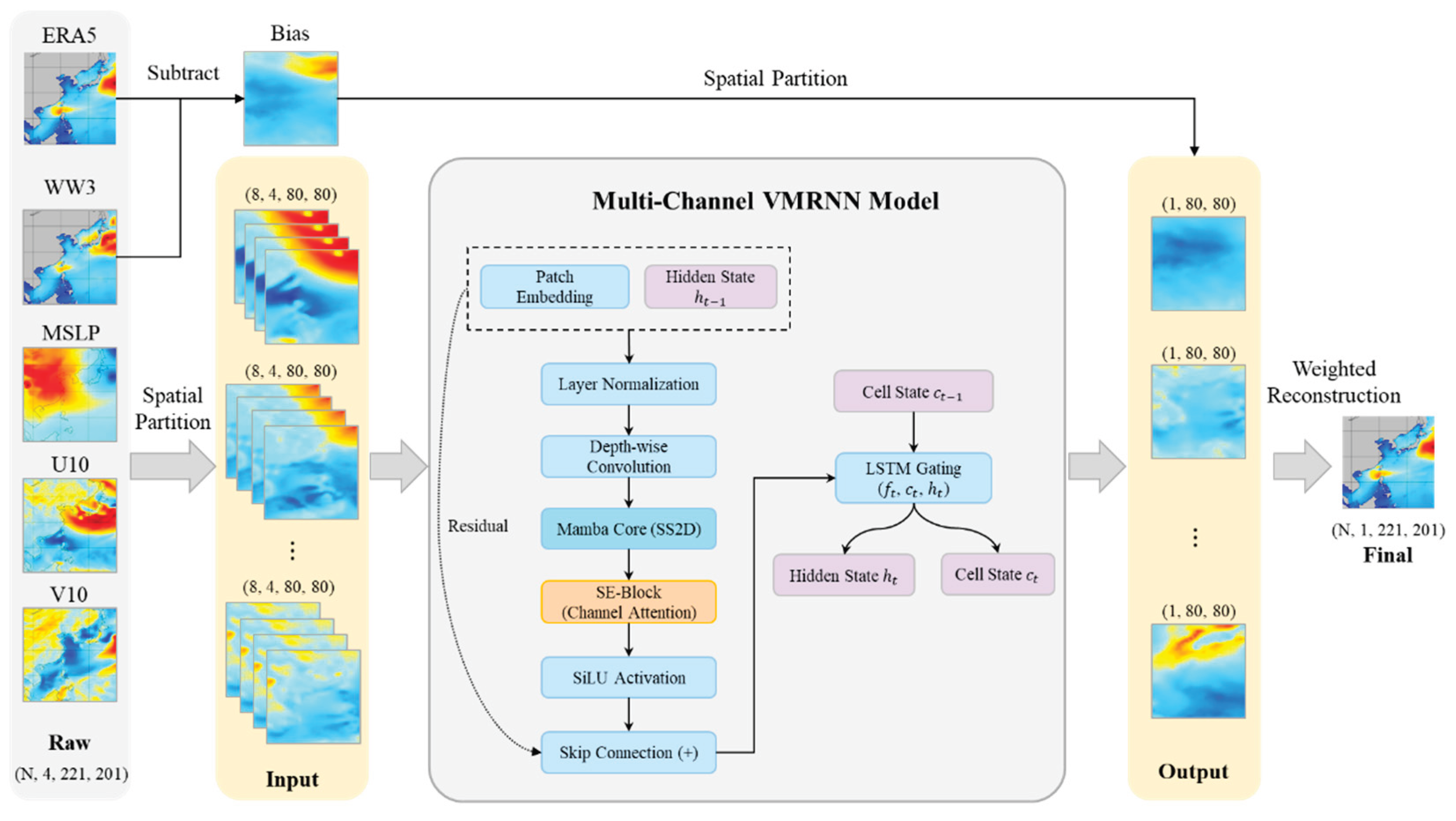
Figure 2.
Study area and partitioning method.
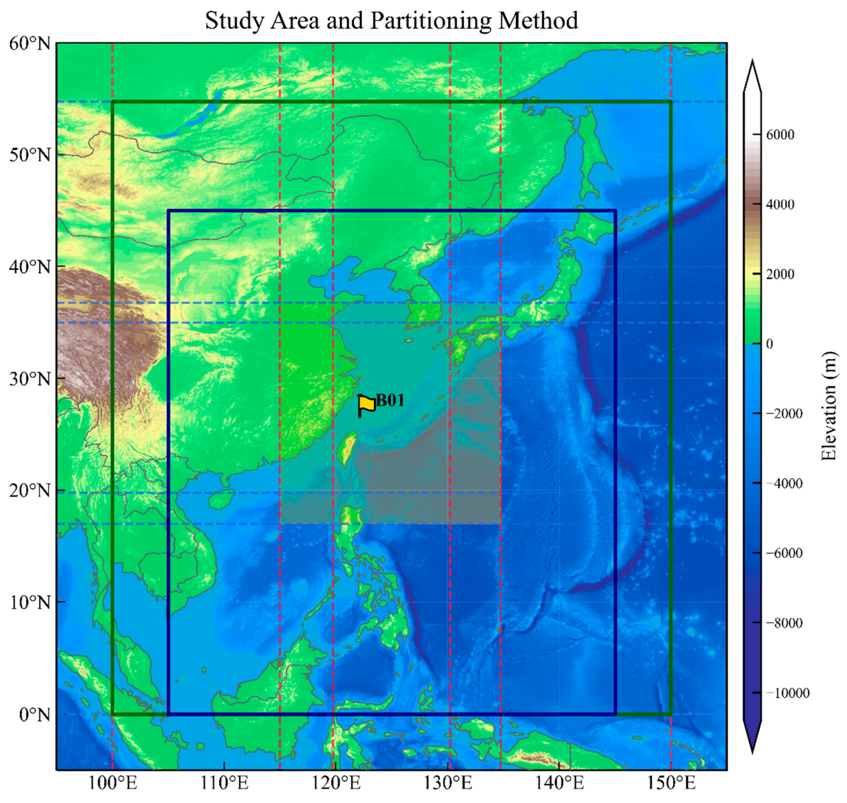
Figure 3.
Sample dataset construction using TSW method.
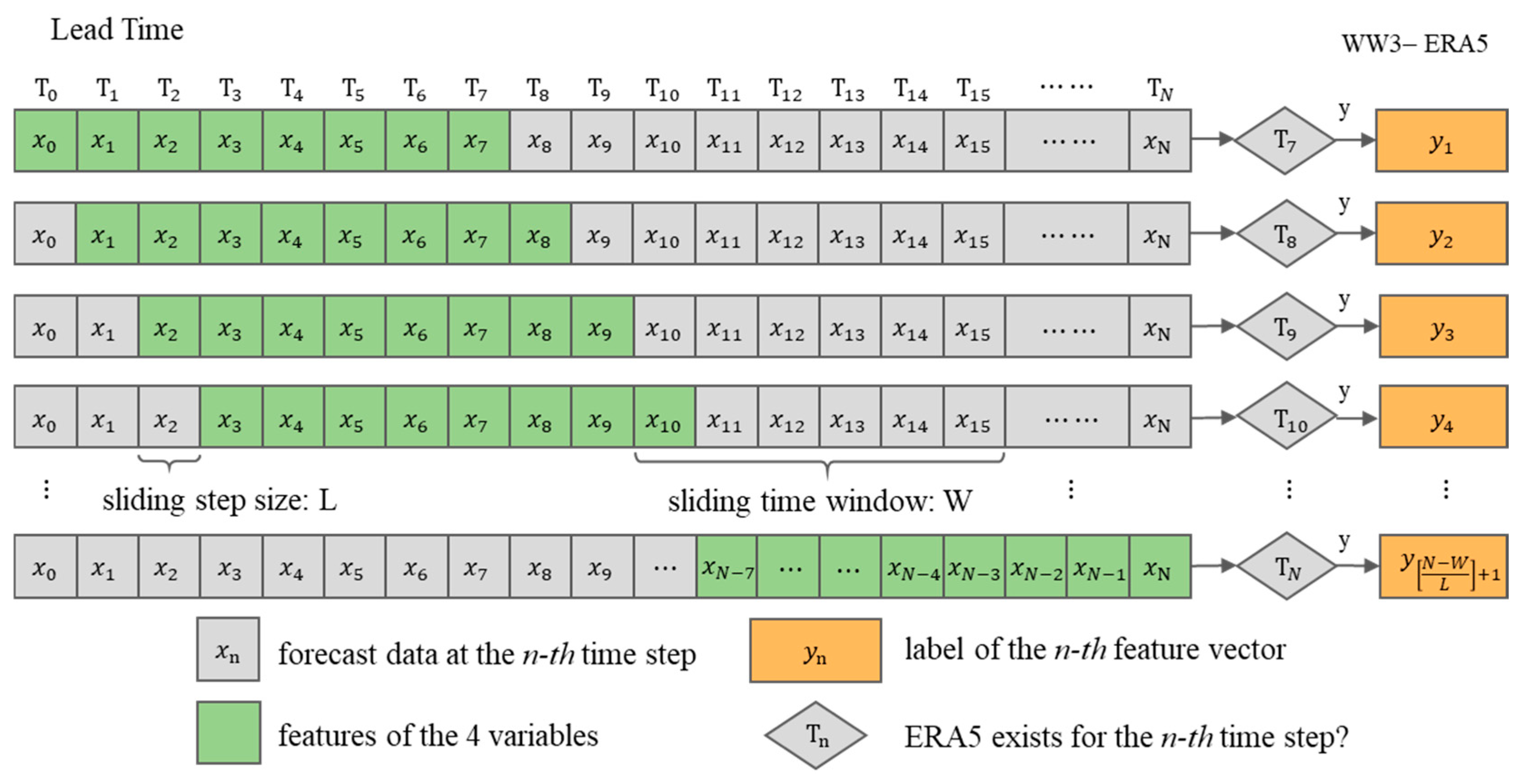
Figure 4.
Structure of the VMRNN integrated with channel attention mechanism: (a) Overall architecture; (b) VMRNN cell detail.
Figure 4.
Structure of the VMRNN integrated with channel attention mechanism: (a) Overall architecture; (b) VMRNN cell detail.
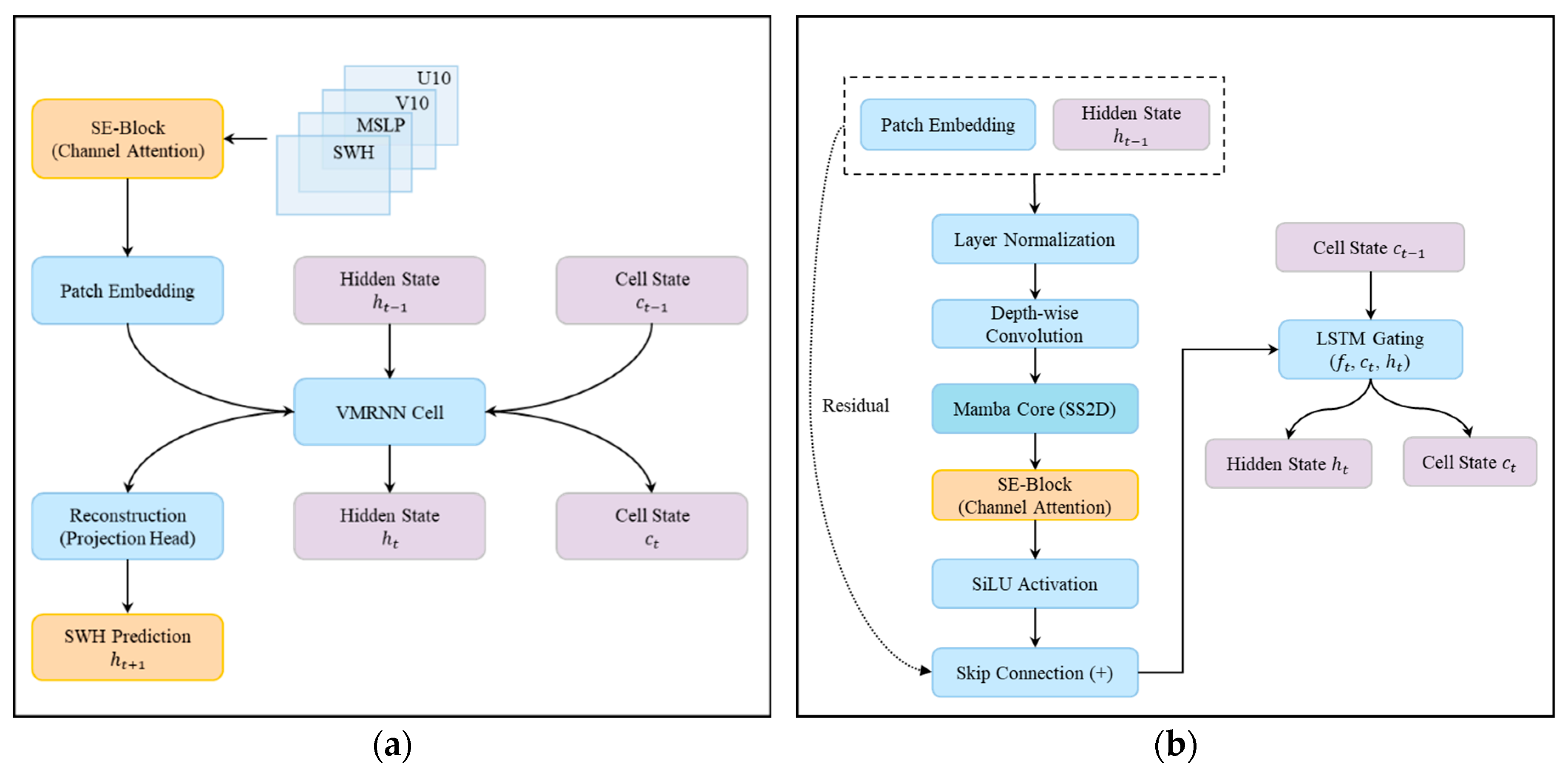
Figure 5.
Time series of average RMSE for SWH forecast by various models.
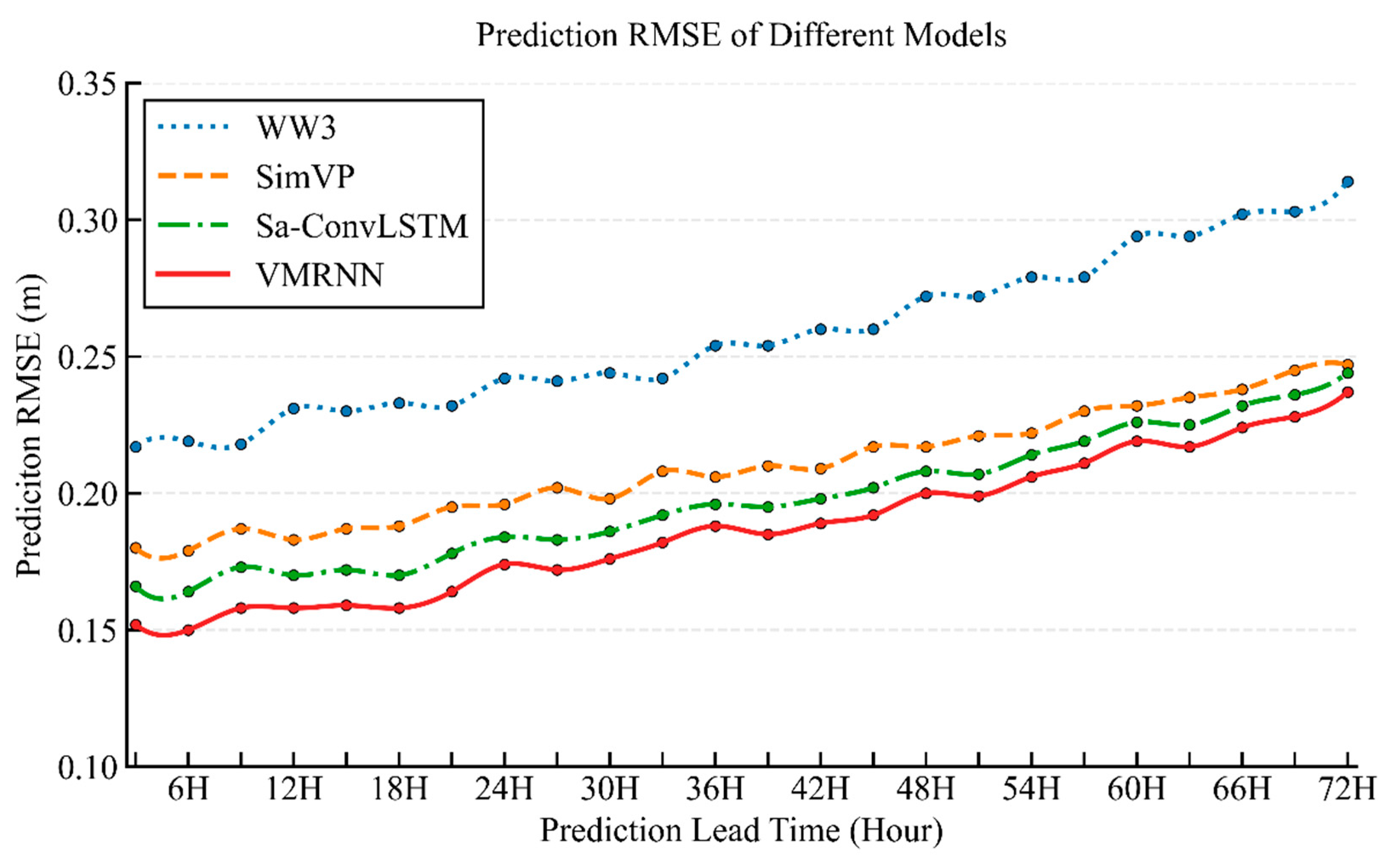
Figure 6.
Spatial distribution of RMSE for SWH Forecasts by different models at various lead times: (a)-(d) 24h prediction of WW3, SimVP, Sa-ConvLSTM, VMRNN; (e)-(h) 48h prediction of WW3, SimVP, Sa-ConvLSTM, VMRNN; (i)-(l) 72h prediction of WW3, SimVP, Sa-ConvLSTM, VMRNN.
Figure 6.
Spatial distribution of RMSE for SWH Forecasts by different models at various lead times: (a)-(d) 24h prediction of WW3, SimVP, Sa-ConvLSTM, VMRNN; (e)-(h) 48h prediction of WW3, SimVP, Sa-ConvLSTM, VMRNN; (i)-(l) 72h prediction of WW3, SimVP, Sa-ConvLSTM, VMRNN.
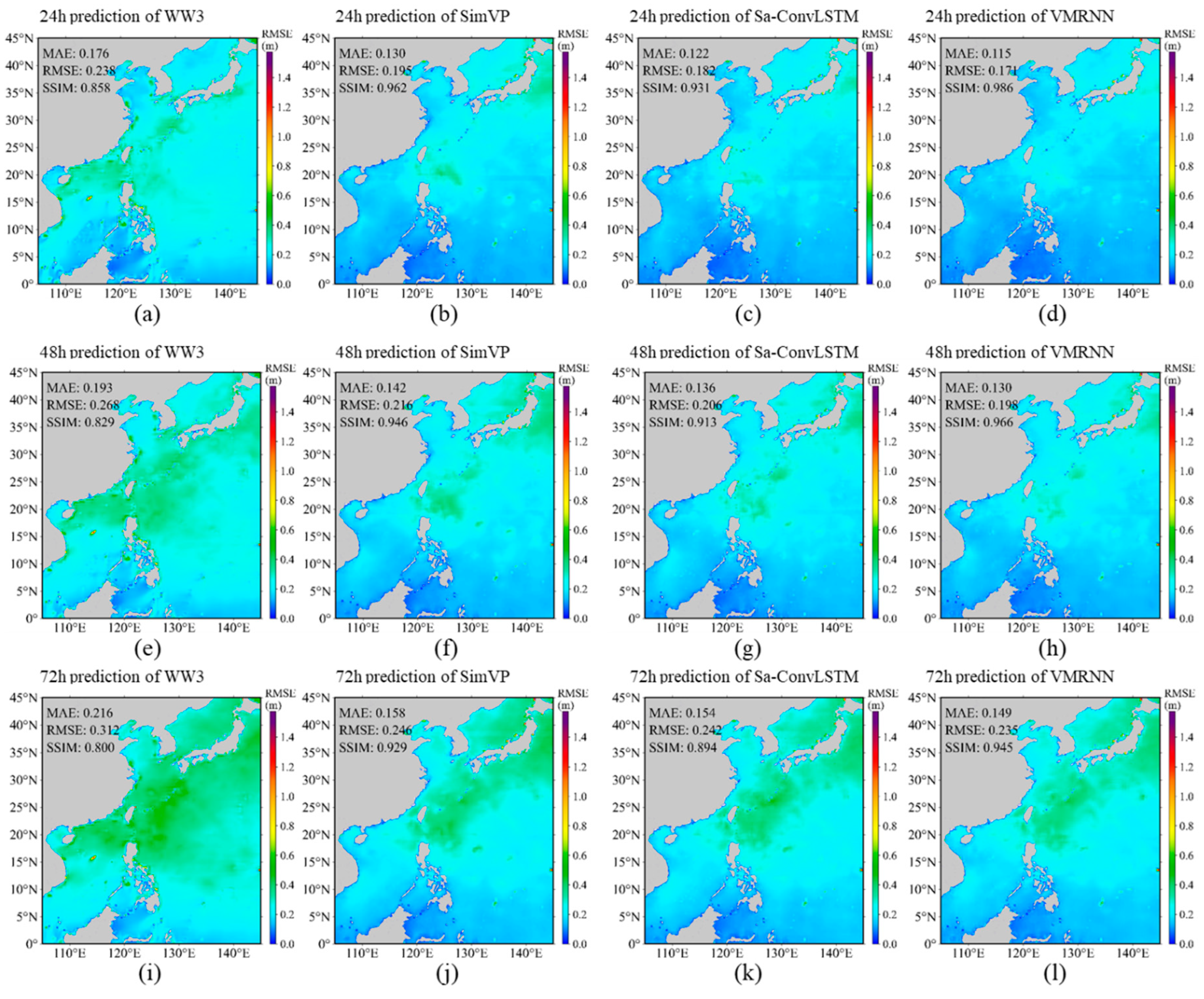
Figure 7.
Bar chart of prediction RMSEs for SWH at different levels.
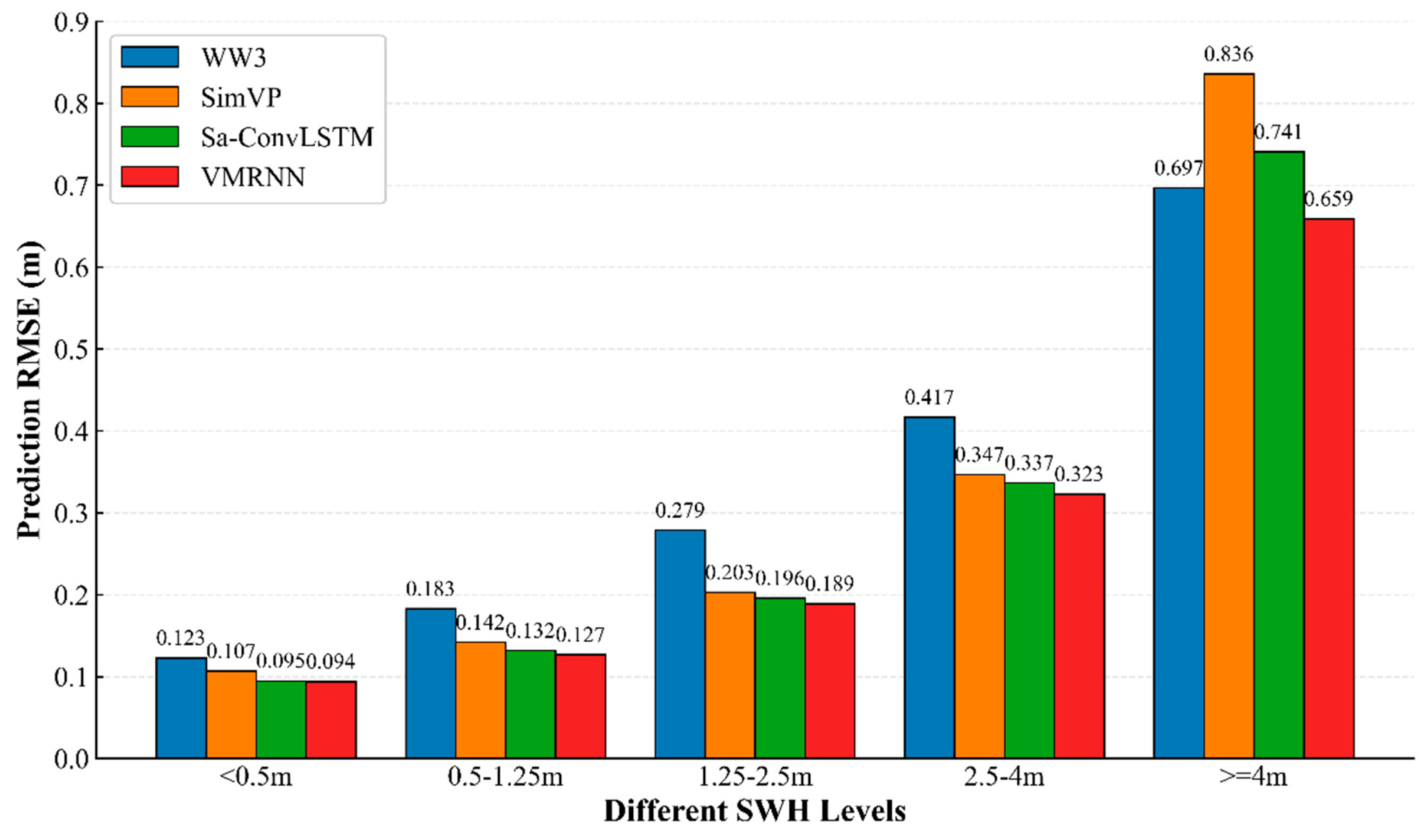
Figure 8.
Time series curves of TS and FAR for prediction of waves Above 4 m: (a) TS values of different models; (b) FAR values of different models.
Figure 8.
Time series curves of TS and FAR for prediction of waves Above 4 m: (a) TS values of different models; (b) FAR values of different models.
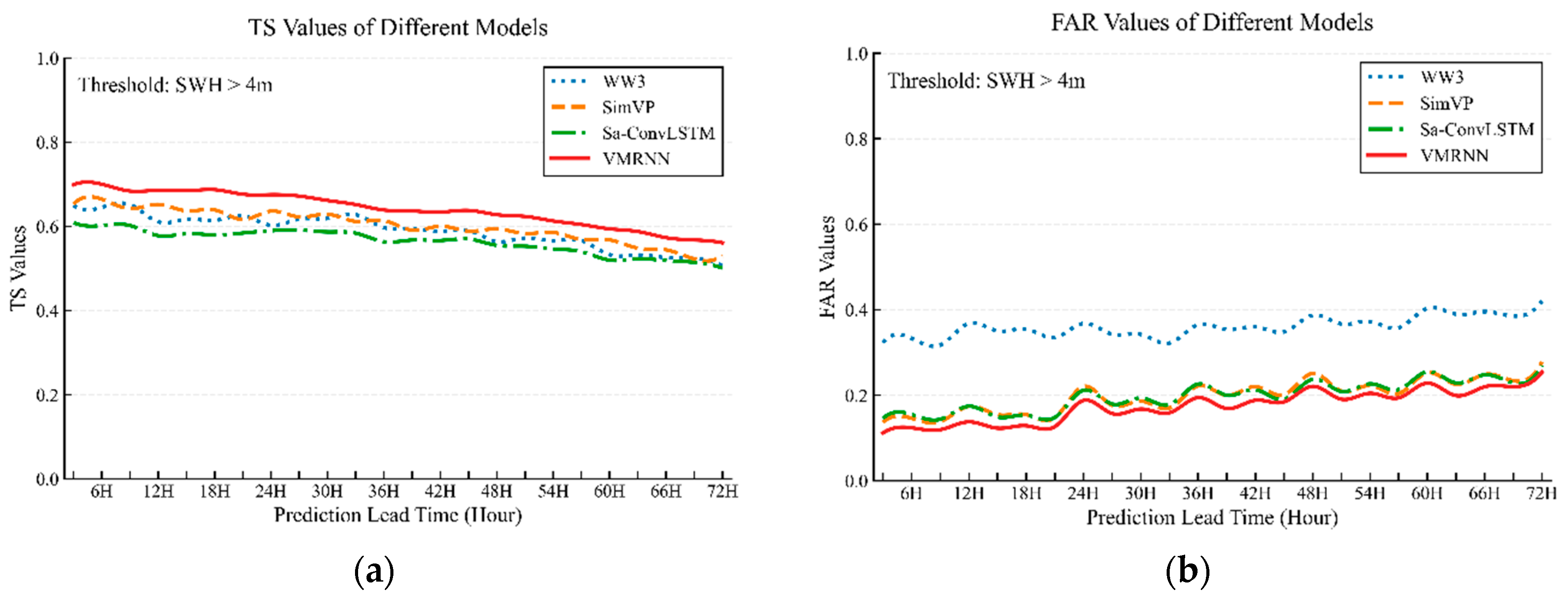
Figure 9.
Scatter plot of model results versus In-Situ observations at different prediction lead times: (a)-(c) scatters of day 1 for ERA5, WW3, VMRNN; (d)-(f) scatters of day 2 for ERA5, WW3, VMRNN; (g)-(i) scatters of day3 for ERA5, WW3, VMRNN. Day 1 (3–24 h); Day 2 (27–48 h); Day 3 (51–72 h).
Figure 9.
Scatter plot of model results versus In-Situ observations at different prediction lead times: (a)-(c) scatters of day 1 for ERA5, WW3, VMRNN; (d)-(f) scatters of day 2 for ERA5, WW3, VMRNN; (g)-(i) scatters of day3 for ERA5, WW3, VMRNN. Day 1 (3–24 h); Day 2 (27–48 h); Day 3 (51–72 h).
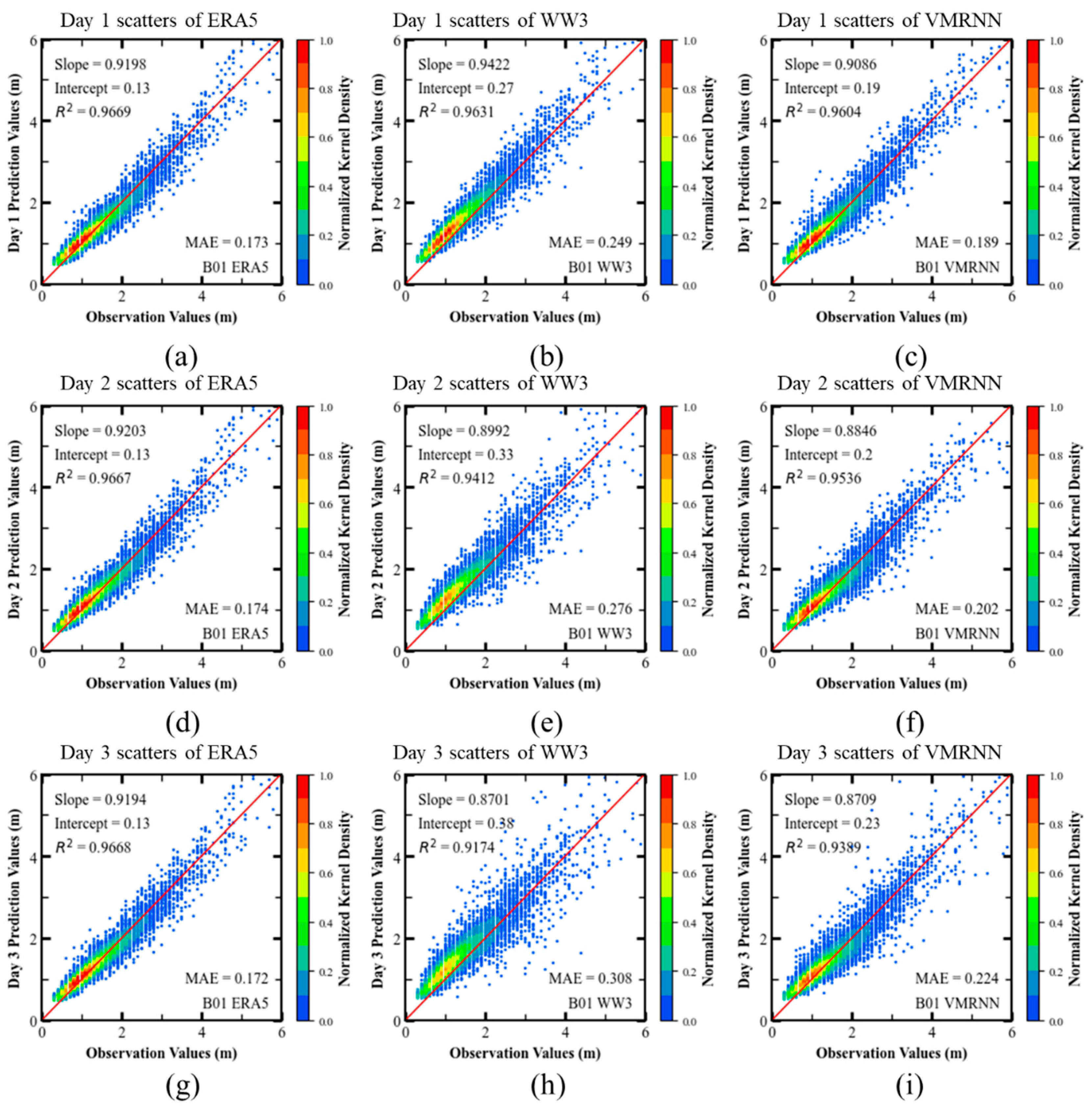
Figure 10.
Violin plots comparing model results against in-Situ data at different prediction lead times: (a)-(c) violin plots of day 1 for ERA5, WW3, VMRNN; (d)-(f) violin plots of day 2 for ERA5, WW3, VMRNN; (g)-(i) violin plots of day 3 for ERA5, WW3, VMRNN. Day 1 (3–24 h); Day 2 (27–48 h); Day 3 (51–72 h).
Figure 10.
Violin plots comparing model results against in-Situ data at different prediction lead times: (a)-(c) violin plots of day 1 for ERA5, WW3, VMRNN; (d)-(f) violin plots of day 2 for ERA5, WW3, VMRNN; (g)-(i) violin plots of day 3 for ERA5, WW3, VMRNN. Day 1 (3–24 h); Day 2 (27–48 h); Day 3 (51–72 h).
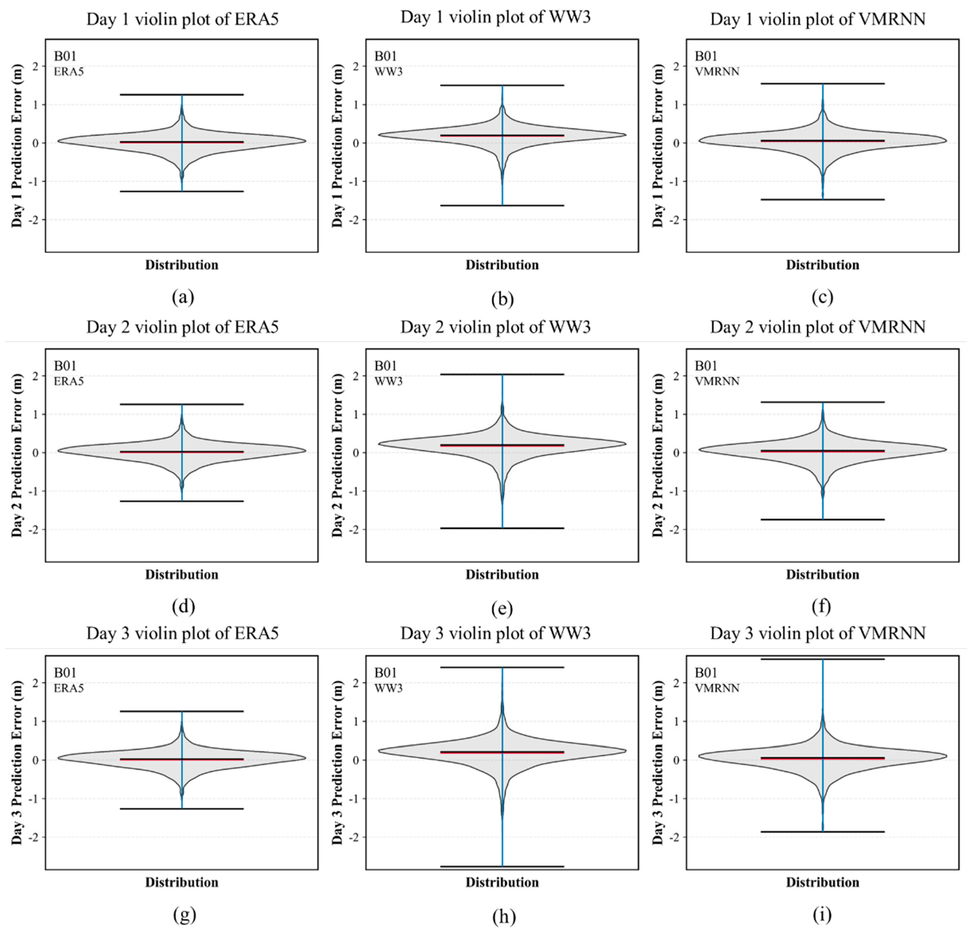

Table 1.
Overall of related studies on wave prediction bias correction using AI models.
| Correction Model | Label Type | Base Model |
| ANN [46] | Location | INCOIS |
| MLP, GBT [47] | Location | State-owned System |
| Sa-ConvLSTM [36] | Field | SWAN |
| BRT, ANN [15] | Location | SWAN |
| Ef-ANN [48] | Location | WW3 |
| Sa-Encoder-Decoder [49] | Field | WAM |
| EW, BTFF, WAF [50] | Field | WW3 |
| CNN, LSTM [51] | Field | SWAN |
Table 2.
Data and data sources.
| Data Type | Variable |
Temporal Coverage |
Temporal Resolution |
Spatial Resolution |
Data Source |
| Wave forecast data | SWH | 2019.02-2024.12 | Once daily, 3-hourly interval, 72-hour lead time | 0.25° | NMEFC |
| Wind forecast data | U10 1 and V10 2 | 2019.02-2024.12 | Once daily, 3-hourly interval, 72-hour lead time | 0.25° | PanGu-Weather |
| Pressure forecast data |
MSLP 3 | 2019.02-2024.12 | Once daily, 3-hourly interval, 72-hour lead time | 0.25° | PanGu-Weather |
| Wave reanalysis data | SWH | 2019.02-2024.12 | Hourly | 0.25° | ECMWF |
| Buoy observation data | SWH | 2023.01-2024.12 | Hourly | - 4 | MNR 5 buoy |
1 10-m zonal (u) wind component; 2 10-m meridional (v) wind component; 3 mean sea level pressure; 4 indicates not applicable; 5 Ministry of Natural Resources of China.
Table 3.
Spatial partition method.
| Rows | Latitude | Columns | Longitude | |
| a | 0.00°N – 19.75°N | x | 100.00°E – 119.75°E | |
| b | 17.00°N – 36.75°N | y | 115.00°E – 134.75°E | |
| c | 35.25°N – 55°N | z | 130.25°E – 150.00°E |
Table 4.
Statistical RMSE of predictions from different models at various lead times for B01 Buoy (Unit: m).
Table 4.
Statistical RMSE of predictions from different models at various lead times for B01 Buoy (Unit: m).
| Lead Time | ERA5 | WW3 | SimVP | Sa-ConvLSTM | VMRNN |
| 6h | 0.233 | 0.293 | 0.288 | 0.274 | 0.256 |
| 12h | 0.233 | 0.302 | 0.285 | 0.267 | 0.260 |
| 18h | 0.227 | 0.304 | 0.300 | 0.266 | 0.251 |
| 24h | 0.231 | 0.332 | 0.312 | 0.272 | 0.266 |
| 30h | 0.234 | 0.340 | 0.319 | 0.277 | 0.269 |
| 36h | 0.232 | 0.343 | 0.306 | 0.283 | 0.277 |
| 42h | 0.230 | 0.352 | 0.320 | 0.288 | 0.280 |
| 48h | 0.232 | 0.381 | 0.331 | 0.293 | 0.292 |
| 54h | 0.237 | 0.396 | 0.350 | 0.302 | 0.298 |
| 60h | 0.232 | 0.392 | 0.331 | 0.309 | 0.301 |
| 66h | 0.235 | 0.388 | 0.343 | 0.319 | 0.317 |
| 72h | 0.227 | 0.441 | 0.378 | 0.335 | 0.343 |
| Average | 0.232 | 0.355 | 0.322 | 0.290 | 0.284 |
Disclaimer/Publisher’s Note: The statements, opinions and data contained in all publications are solely those of the individual author(s) and contributor(s) and not of MDPI and/or the editor(s). MDPI and/or the editor(s) disclaim responsibility for any injury to people or property resulting from any ideas, methods, instructions or products referred to in the content. |
© 2026 by the authors. Licensee MDPI, Basel, Switzerland. This article is an open access article distributed under the terms and conditions of the Creative Commons Attribution (CC BY) license (http://creativecommons.org/licenses/by/4.0/).
Copyright: This open access article is published under a Creative Commons CC BY 4.0 license, which permit the free download, distribution, and reuse, provided that the author and preprint are cited in any reuse.