

Submitted:
08 May 2026
Posted:
09 May 2026
You are already at the latest version
Abstract
Optical imaging is among the safest and most highly impactful biomedical imaging modalities. Aberration in the optical imaging systems leads to distorted images. This distortion is almost nonlinear and hence affects the relative size, intensity and appearance of image details. Image aberration has many types with some or all of them can be imposed on the image based on the quality of the imaging system and/or surrounding conditions. Many approaches have been introduced to remove or minimize aberration from optical images. If the transfer function of an imaging system and the function of the noise added during the imaging process are known, then an ideal image can be obtained from the image produced by this system. The point spread function (PSF) of the optical imaging system is the image it produces for a point object. PSF is the observable form of the transfer function. The transfer function itself is the exit pupil function or typically the system aberration. The nonlinearity and multiplicity of the aberration imposed on the image together with the added noise makes it difficult to obtain the transfer function from the degraded images. In this work, optimization and global search techniques are utilized in an iterative image restoration algorithm. The proposed technique updates an initially suggested solution of transfer function by optimizing the aberration coefficients. The final solution of the transfer function and hence the PSF is reached when the optimum restored image is obtained. The proposed algorithm is validated by a testing image and then its performance is assessed by a set of aberrated images with different degradation. The results obtained in this work showed 100% success rate to obtain the PSF.
Keywords:
optimization
; global search
; aberration correction
; image restoration
1. Background and Literature Review
In the medical field, optical imaging remains a vital imaging tool for many biological and physiological studies. A main issue in optical imaging is the aberration imposed on the image by the imaging system which leads to image distortion. The aberration comes from the limitations of the design of optical components, the surrounding conditions and/or the physical characteristics of the imaged objects [1,2]. The lens itself is an imaging system, although sophisticated systems often have many components. So, in optical imaging, the lens is generally used to refer to the imaging system.
A collimated beam has a planer wavefront that keeps its shape when it propagates through a homogeneous and uniform medium. Passing through a non-planar optical element or lens, this wavefront gets distorted by aberration. Aberration is due to the deviation of rays, departing from a single point on the object, from their expected paths. So, rays from a single point on the object reach the sensor, or the image plane, at different points with different intensities. So, a point on the object is not represented by a point on the image but rather by a shape, however, the point itself can still be observed in this shape on the image. If this is applied to all points of the object, intuitively, it leads to the formation of an image distorted by rays’ deviations [3,4].
The image plane is the plane on which the best image can be formed. The image is fully described by the spatial distribution of amplitude and phase. But the observable image is the spatial distribution of light intensities simulating the distribution of light intensities coming from the object. Taking into account that light intensity is given by the squared amplitude of the beam, denote the 2D object and the image functions by and respectively. An ideal system produces an ideal image . As a system, the output of the optical imaging system is given by,
where and are respectively the system transfer function and the noise added to the image by the environment. In the frequency domain, it is given by,
The formula of the produced image in (1) comes from the fact that each point on the object sends a cone of light covering the full extent of the lens. This means that each point on the lens collects (i.e., adds) rays from all points on the object and sends them to different points on the image plane. A cone of rays emanates from one point on the object, passes the lens and is focused onto the image plane. If the system is ideal, it focuses this cone to a single point on the image plane and hence produces an ideal image. But nothing created by humans is ideal and the cone is focused to a shape (e.g., a spot) rather than a point. This happens with cones from each point on the object. So, it leads to an overall distorted image. The noise is added to the image by the surrounding conditions. This definition means that the image is the convolution of the object function and the transfer function plus the noise as described by (1).
So, the transfer function is basically the image of a point source if no noise is added. The point source is represented by a delta or an impulse function and hence the transfer function is also called the impulse response of the system. So, for a point source,
where, is a point object given by the delta or impulse function, (Point Spread Function) is its observable image function given by the intensity distribution over the space of the image. The transfer function is the spatial distribution of light amplitude and phase. To clarify, consider a planar uniform wavefront passing through an optical element or system, it gets deformed due to the lens shape, to a non-planar wavefront that reaches the sensor with different intensities i.e. non-uniform. The shape of the lens pushes rays to pass slower or faster than each other with slightly different deviations leading to an aberrated wavefront. So, the aberration pattern is the deviation or spatial error function between the planar wavefront and its deformed wavefront. This wavefront deviation or aberration pattern is denoted by an in the Cartesian and polar coordinates respectively. In the frequency domain the aberration pattern is described by the phase differences between the shape of the original and the deformed wavefronts as . Consequently, it’s easier to be studied in the frequency domain [6]. The lens aberration is imposed to any imaged object either it is a point or any other shape and is denoted by,
where is the phase difference and are the spatial frequencies in the and directions respectively.
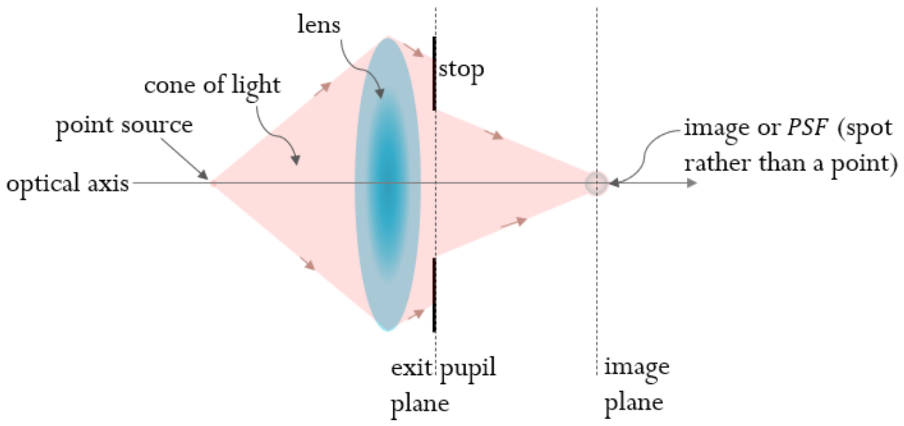
To decrease the lens aberration, a stop aperture is placed after the lens, as shown in Figure 1. This allows only paraxial rays to pass to the image plane. Paraxial rays undergo less deviations than peripheral rays. The stop aperture is called the exit pupil. So, the aperture multiplies the wavefront by a zero-one function outside and inside its circumference respectively. This is just an apodization function and given by,
where is the radius of the pupil. The aberration and consequently, the transfer function is typically measured after the exit pupil and that’s why it is called the pupil function. For a circular aperture, the pupil function is given in the polar coordinate by,
where , and are respectively the notations of the apodization function, aberration pattern and the transfer functions in the polar coordinates.
From the above analysis and as provided in [6], the transfer function in the frequency domain is given by,
Different optical elements impose different aberration patterns. For a single lens, the point object appears as a shape in the image. For a 3D image, this shape may be a sphere, an ellipsoid, etc..... For a 2D image, the point object may appear in the image as a spot, a comma, etc.... as shown in figure 1. As an example, if the transfer function is a Gaussian spot, then the narrower the spot the sharper the PSF and the better the lens. That’s why the image of a point object is called the Point-Spread Function, PSF as it indicates how spread the image of a point is. [5].
Figure 1.
A schematic diagram of a simple optical imaging system showing the point object, the exit pupil and the PSF.
Figure 1.
A schematic diagram of a simple optical imaging system showing the point object, the exit pupil and the PSF.
However, the mathematical foundation of aberration in the spatial domain is done starting from the fact that the aberration is the wavefront deviation. Since the exit pupil is commonly circular, the Zernike polynomials which are polynomials defined over a unit circle, are commonly used to describe the aberration wavefront . According to the shape of the point object in the image, aberration has many types. Each type can be acceptably fitted by a term of the Zernike polynomial. Details of different Zernike polynomials and different aberration types are provided in [7,8,9]. A lens or an optical imaging system imposes multiple types of aberration on the produced image [10]. So, the wavefront aberration is given in the cartesian and polar coordinates by,
where is the kth Zernike term, is the coefficient of the kth term and is the number of Zernike terms describe the aberration as accurate as possible. The aberration types are usually sorted in triangular figures called aberration pattern. On the apex, zeroth order which has only one pattern called piston. The first order has 2 patterns, tilt-x and tilt-y. The second order has 3 patterns, astigmatism and defocus. The third order has 4 patterns, trefoil-x, trefoil-y, coma-x and coma-y and so on [10].
Theoreticaaly, the number of Zernike terms but usually few types or even one type of aberration is dominant for a lens or a system. These dominant types have the greatest coefficients and are enough to be defined for aberration correction [10]. In [10], the authors provide the details of 15 types of aberration representing the first 5 orders. Table 1 presents 5 of these 15: piston, tilt or prism along the x-direction, coma in the x-direction, defocus and primary spherical with their formulae in the polar and Cartesian coordinates. Some other patterns of these 15 are used in this work and are presented in Table 2.
From (6) and (7) and over the pupil area,
To improve the optical image, the researchers provided many techniques to remove or minimize the aberration. A single optical element or system can impose one or more aberration types on the produced image. The imposed aberration types are usually unknown and have different coefficients. This makes it too difficult to remove aberration, but the good news is that one or two types of imposed aberration are dominant according to the values of their coefficients. Trials are usually done to remove such dominant aberration types in a process called aberration correction [3,4,5,6].
From (6), the system transfer function is the exit pupil function with aberration represents the phase of such function. So, knowing the transfer function, the aberration can be removed using the inverse function. But practical handling is not always that simple because of the nonlinearity of aberration as well as the noise added to image during the capturing [9].
A lot of research has been conducted to reduce the aberration of optical images either by digital image processing or using the adaptive optics kits aligned with the optical imaging system. The use of adaptive optics is expensive and adds complexity to the system either regarding the size or alignment.
On the field of digital image processing, many researchers introduced computational methods to estimate the original image from the aberrated image with or without knowing the imposed aberrations. The new approaches use a deconvolution algorithm to deblur the aberrated images [11,12,13]. If the transfer function of the imaging system is known, the reconstructed image is simply obtained by deconvolution of the aberrated image with the transfer function. The advantage of using post-processing by digital algorithms can be extended to enhance the resolution and contrast of the image and to denoising the image with no cost. Unfortunately, the transfer system is almost not known. Using blind deconvolution approaches suggested by many studies is not guaranteed to give an accurate image reconstruction [14].
Many modern approaches to computational aberration correction are based on deep learning (DL) methods. For example, Li trained a DL model with a set of optical lenses and their corresponding images [15]. Their system takes as input the aberrant image and the PSF map, and outputs a corrected image. In another example of DL-based aberration correction, Eboli reported a “blind” optical aberration compensation technique in which chromatic aberrations are corrected using a convolutional neural network trained to minimize residuals between the red/green and blue/green planes [16]. More recently, Gong reported a DL-based approach in which the physical properties of optical lenses were incorporated into an aberration correction network [17].
While the most recent examples of aberration correction incorporate a physics-informed approach, these techniques have largely avoided differentiable optical models, or discussion of fundamental aberration theory with Zernike coefficients. Liaudat proposed such a model in which the wavefront itself is considered, not merely the pixels of the image [18]. Another recent example that considers Zernike coefficients in aberration correction is the work of Sauniere, in which the team used a D L approach to extract Zernike coefficients from a low-resolution PSF image [19]. These DL approaches are limiting in that they require advanced computing power. There remains a gap in the literature for advanced aberration correction methods that do not rely on DL. Such an analytical system would speed up aberration correction, a proposition that would be useful in many areas where optical imaging is employed. To test the validity of the proposed method a reference high quality image is used, a degraded version is obtained by convolving the reference image by a known aberration pattern and obtaining the restored image and the test pattern. Through visual investigation, the restored method is identical to the reference image and the induced aberration pattern is identical to the imposed testing pattern.
2. Methods
As the observable image of a point object, the PSF is commonly used to assess the quality of the imaging system because it describes how a point object is represented (or get spread) in the produced image. From (3), the PSF is the square of the modulus of the system’s transfer function. So, the transfer function and consequently the PSF differs from system to system, and basically from one optical element to another, based on the quality of the materials, fabrication methods and alignment. It’s worth mentioning that the Fourier transform of the PSF is the OTF abbreviated from Optical Transfer Function while MTF or is the Fourier transform of [20].
Image improvement is mostly done digitally by applying image processing algorithms to the images. In most cases, image processing is applied while the transfer functions are unknown. Filtering techniques are applied to the images for many reasons including restoration. Theoretically, image restoration means obtaining the ideal image from a given distorted image . Practically, the ideal image can’t be obtained but rather an estimate of it that must be as improved as possible. So, image restoration leads to aberration correction. Image restoration can be done by digital filtering in the spatial domain to obtain an estimated image or in the frequency domain to estimate and then converting it to the spatial domain. It is usually recommended to apply digital filters in the frequency domain to remove the complexity of convolution in the spatial domain [21].
Wiener filter is known for its efficiency in image restoration and obtaining the spatial deformation exerted to an image taking noise into consideration. The Wiener filtering process in the frequency domain is given by,
where is the complex conjugate of , is a thresholding small value applied on to avoid the infinity mathematical result, is the noise to signal power ratio calculated from the prior knowledge of both the noise and the original object . can be empirically selected in case of no prior knowledge of the original image or object and noise. It can also be set to zero in case of the absence of noise [22]. In the field of digital image processing, the system transfer function is called the degradation function because an image produced by a system, is degraded by the effect of its transfer function.
As stated in [22], it is possible to restore from two versions of its distorted image and . This process is done iteratively to get more improved estimates . In the frequency domain this restoration process is given by,
where and are the Fourier transform of two versions of , and are the corresponding MTF or degradation functions. For the optical imaging systems, MTF is given by the apodization and the aberration as driven above in (6). The process is done iteratively until reaching the best solution. While iterating, the transfer functions and are updated and consequently . The iteration is done, in a converging fashion, until reaching the optimum solution.
Initial solutions for and are suggested and consequently a first solution of . An objective function representing the difference between the estimated and the given image is calculated to check the convergence of the process. According to the value of the objective function, the coefficients of the Zernike terms composing the transfer functions are updated and consequently, , and . Using an array, , of values representing the coefficients of the Zernike terms, the process continues by an optimization and global search technique that searches the Zernike coefficient domain until reaching for the optimum coefficient. The optimum Zernike coefficient leads the optimum solution of by which the optimum solution of can be estimated as follows,
The process ends at this point or completing the pre-set number of iterations.
The objective function used in this work is the grand sum error representing the difference between the estimated image and the given image. The grand sum error objective function is given by,
where and are the grand summation of the squared pixel-wise difference between the corresponding estimated and the degraded images. Squaring the difference is done to overcome the sign issue. So, for a Zernike coefficient , the grand sum errors are given by,
According to (13), the optimum solution is obtained at the optimum value C at which gives minimum value of . For a limited number of executions, the range of the Zernike coefficients lies between a lower bound and an upper bound and a function tolerance, , is set to reach the minimum objective error such that,
Figure 2 shows a flow chart of the proposed method where the execution stops at the iteration if the following condition is satisfied,
3. Implementation and Testing
To test the validity of this work, the high-quality microscopic image shown in Figure 3 is used as a reference or an original image . Considering a zero-noise function, a degraded or an input image is obtained by convolving the reference image by a known transfer function as follows,
Over the area of the pupil where apodization function equals 1, substitute form (10) into (15),
According to the phase diversity method [6,23], the aberration function and hence can be chosen as one or a combination of multiple aberration patterns and imposed on the reference image.
Same method is followed to obtain two versions and from the input image by degrading it by two known aberration patterns and respectively. The algorithm is then applied to obtain the optimum estimate and the corresponding aberration pattern .
The generated test images are shown in Figure 3 where the reference image is degraded by a spherical aberration pattern to get the input image . For simplicity, the first known aberration pattern is the piston type and the second is a quadratic term particularly a defocus aberration. So, from Table 1,
The workflow of the proposed algorithm was implemented from the above equations and applied to graylevel images and graylevel aberration patterns. Figure 3 shows a diagram representing the workflow of the proposed method. The algorithm was implemented in MATLAB which ran in a platform of an Intel (R) Corei7 CPU (2.60 GHz) with 16 GB RAM.
A nonlinear optimization algorithm is implemented to search for the best Zernike coefficients correspond to the minimum error function. The MATLAB’s Global Optimization Toolbox is used to search for the optimum Zernike coefficients in their domain. The built-in MATLAB function “fmincon” is a nonlinear programming solver that uses a sequential quadratic programming (SQP) method.
4. Assessment of the Proposed Method
To assess the success rate of the proposed framework, a set of synthetically aberrated images were fed to the framework, their corresponding transfer function were obtained and visually compared to the used patterns. The aberrated images and the estimated aberration patterns are shown in Figure 5 and 6 respectively.
5. Results and Discussion
Local minima in the space is one of the potential problems in the search process. During the search algorithm, the optimizer may give wrong results due to the existence of many local minima. Figure 4 demonstrates real examples of the presence of local minima for the 1D and 2D Zernike coefficient spaces respectively.
The multi-start points approach is an effective solution for the problem of local minima. This approach is used with the MATLAB’s optimizer to make sure that it does not escape the global minimum point.
A numerical measure for the similarity between the estimated image and the reference image is tried as the grand sum of the absolute of the difference between their pixel-by-pixel values. This error measure is given by,
But the values obtained for need a huge number of test images to get a reliable threshold upon which the success of the process can be decided.
Also, a 2D array representing the difference between the reference and estimated image was displayed to see what it reveals. This array is given by,
No information can be obtained from the image represented by the array from which a formula can be deduced as a measure for the similarity between the reference and the estimated image.
So, visual inspection and comparison between the estimated and the reference image is fair enough to be used to assess their similarity. Same analysis applies to assessing the similarity between the aberration pattern used to get the input image and the estimated aberration pattern.
As shown in Figure 3, the testing image is obtained by degrading the reference image by a spherical aberration pattern, the estimated image looks very similar to the reference images. Also, the estimated aberration pattern is visually identical to the spherical aberration pattern used to get the input image. This means that the system is valid and can be assessed by more images with different degradation patterns.
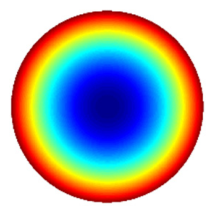
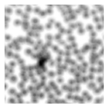
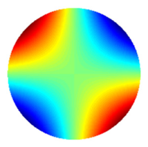
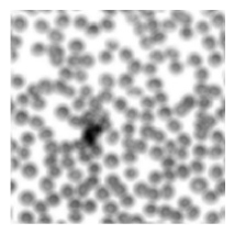
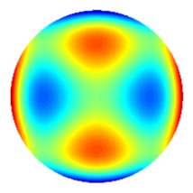
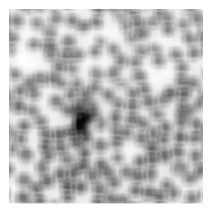
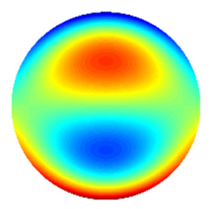
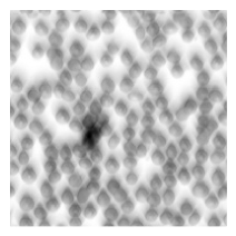
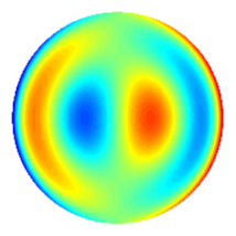
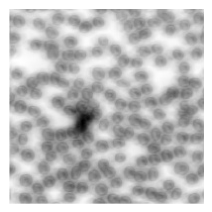
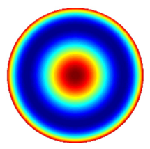
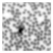
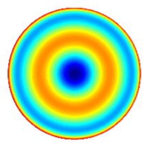
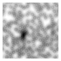
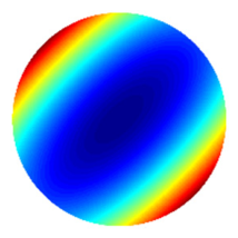
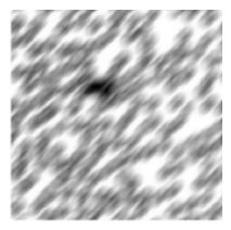
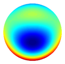
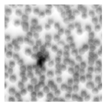
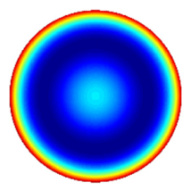
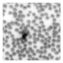
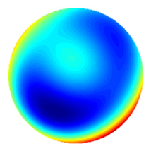
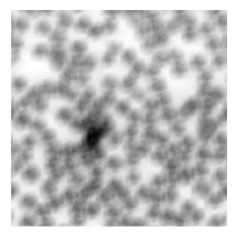
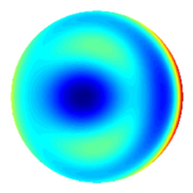
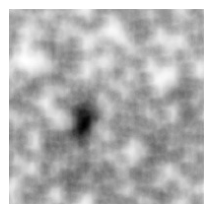
The success rate of the proposed method to obtain the correct aberration pattern(s) is done by applying it to twelve images degraded by different known aberration pattern(s). Seven images were degraded by different single aberration patterns namely (a) Defocus, (b) Primary astigmatism, (c) Secondary astigmatism, (d) Primary coma, (e) Secondary coma, (f) Primary spherical and (g) Secondary spherical. Five images were degraded by different combinations of different aberration patterns namely (h) A combination of defocus with primary astigmatism, (i) A combination of defocus with primary coma, (j) A combination of defocus with primary spherical, (k) A combination of defocus with primary astigmatism, coma, and spherical. (l) A combination of defocus with secondary astigmatism, coma, and spherical.
By visual inspection, the system was able to restore the reference image and the imposed aberration pattern or combination of patterns for the twelve images. The aberration patterns, their formulae, their colored photos and the images degraded by them are shown in Table 2. This showed a 100% success rate for the system performance.
6. Conclusions
Aberration in medical optical imaging is one of the greatest problems as it may distort the acquired images. This distortion affects the relative shapes and sizes of image details. Consequently, improper diagnosis is probable. Aberration can be corrected if the transfer function and the added noise are known. In this work, we provide a robust method to induce the aberration pattern from a given degraded image while restoring the image itself. The induced aberration pattern(s) can be used to restore any image produced by same optical imaging system. The methods combine the optimization, global search and Wiener filter to do the task. The proposed method has a 100% success rate based on 13 images with different degradation functions. The proposed method can be applied to planar x-ray images as well. In future, images taken from different image modalities such as CT and MRI are to be proceed for their transfer functions other than aberration.
Institutional Review Board Statement
Not applicable.
Informed Consent Statement
Not applicable.
References
- Smith, N.; Webb, A. Introduction to Medical Imaging Physics, Engineering and Clinical Applications; Cambridge University Press: New York, 2011. [Google Scholar]
- Ravikumar, S. Effect of optical aberrations on image quality and visual performance. 2009. [Google Scholar]
- Mahajan, Virendra N. Optical Imaging and Aberrations, Part II. Wave Diffraction Optics", Ch.1. Ch.2 and Ch.5; SPIE Digital liberary, 2001. [Google Scholar]
- van Driel, H. M. Modern Optics Notes", Ch. 5, University of Toronto Version: 2.2; 2010. [Google Scholar]
- Solouma, Nahed. Assessment of imaging systems: A tutorial handouts; King Faisal University, 2025. [Google Scholar]
- Fienup, J. R. Phase retrieval algorithms: a comparison. Appl. Opt. 1982, 21, 2758–2769. [Google Scholar] [CrossRef] [PubMed]
- Born, M.; Wolf, E. Principles of Optics; Pergamon press: New York, 1959; pp. 464–466, 767–772. [Google Scholar]
- Wyant, J. C.; Creath, K. Applied Optics and Optical Engineering; Shannon, R., Wyant, J., Eds.; Academic Press: New York, 1992; Volume XI, pp. 28–39. [Google Scholar]
- Wyant, James C. Zernike Polynomials. 2003; College of Optical Science, Arizona university website, viseted on April 2026. [Google Scholar] [PubMed]
- Negm, Noura. The Use of Adaptive Optics to Improve Image Quality of the Wide-Field Transmission Microscopy. a thesis disertation, Cairo University, 2017. Chapter 2. [Google Scholar]
- Ahmad, A.; et al. Real-time in vivo computed optical interferometric tomography. Nat. Photonics 2013, 7, 444–448. [Google Scholar] [CrossRef] [PubMed]
- South, F. A.; Liu, Y.-Z.; Carney, P. S.; Boppart, S. A. Computational adaptive optics of the human retina; SPIE; Volume 9693, pp. 151–155.
- Zhu, D.; et al. Automated fast computational adaptive optics for optical coherence tomography based on a stochastic parallel gradient descent algorithm. Opt. Express 2020, 2 8, 23306–23319. [Google Scholar] [CrossRef] [PubMed]
- Donatelli, M.; Serra-Capizzano, S. Computational methods for inverse problems in imaging; Springer, 2019. [Google Scholar]
- Li, X.; Suo, J.; Zhang, W.; Yuan, X.; Dai, Q. Universal and flexible optical aberration correction using deep-prior based deconvolution. In Proceedings of the IEEE/CVF International Conference on Computer Vision, 2021; pp. 2613–2621. [Google Scholar]
- Eboli, T.; Morel, J.-M.; Facciolo, G. Fast two-step blind optical aberration correction. In European Conference on Computer Vision; Springer, 2022; pp. 693–708. [Google Scholar]
- Gong, J.; Yang, R.; Zhang, W.; Suo, J.; Dai, Q. A Physics-informed Low-rank Deep Neural Network for Blind and Universal Lens Aberration Correction. In Proceedings of the IEEE/CVF Conference on Computer Vision and Pattern Recognition, 2024; pp. 24861–24870. [Google Scholar]
- Liaudat, T.; Starck, J.-L.; Kilbinger, M.; Frugier, P.-A. Rethinking data-driven point spread function modeling with a differentiable optical model. Inverse Probl. 2023, 39, 035008. [Google Scholar] [CrossRef]
- Sauniere, L.; Gillard, W.; Zoubian, J. Decoding optical aberrations of low-resolution Instruments from PSFs: machine learning and Zernike polynomials perspectives. In Space Telescopes and Instrumentation 2024: Optical, Infrared, and Millimeter Wave; SPIE, 2024; Volume 13092, pp. 1262–1274. [Google Scholar]
- Joseph A. Shaw, "Optical system design handout", Montana State University , link, taken on April 9, 2026.
- Umbaugh, S. E. Digital Image Processing and Analysis: Applications with MATLAB® and CVIPtools; CRC press, 2017. [Google Scholar]
- Donatelli, M.; Serra-Capizzano, S. Computational methods for inverse problems in imaging; Springer, 2019. [Google Scholar]
Figure 2.
a Flow chart elaborating the proposed method.
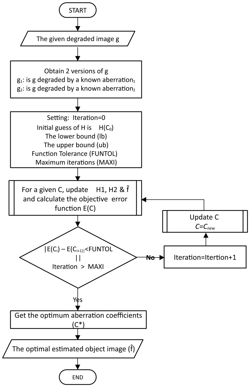
Figure 3.
a process diagram showing the workflow of the algorithm with the images used to test its validity and the estimated optimum image and optimum aberration pattern.
Figure 3.
a process diagram showing the workflow of the algorithm with the images used to test its validity and the estimated optimum image and optimum aberration pattern.
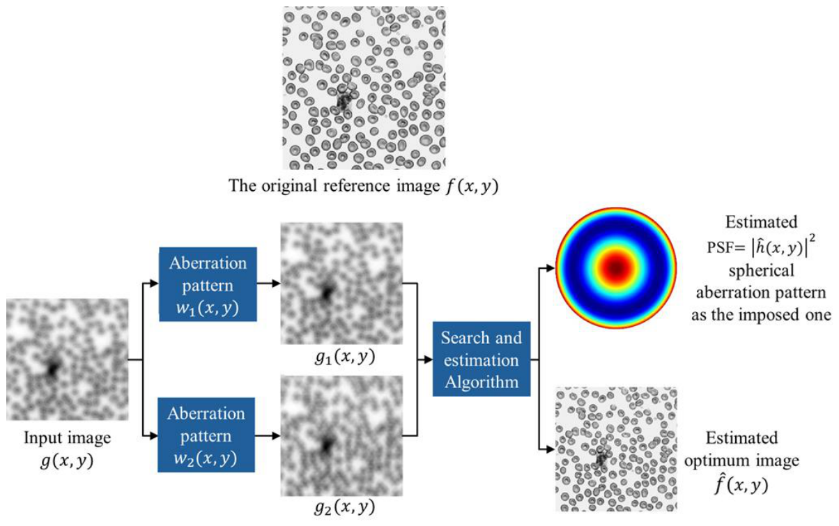
Figure 4.
The demonstration of local minima problem occurred on the error function and may lead to inaccurate results. Upper: for a 1D Zernike coefficient space. Lower: for a 2D Zernike coefficient space.
Figure 4.
The demonstration of local minima problem occurred on the error function and may lead to inaccurate results. Upper: for a 1D Zernike coefficient space. Lower: for a 2D Zernike coefficient space.
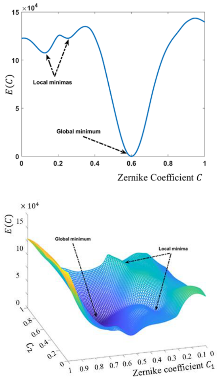

Table 1.
Some common aberration types.
| , order) | Aberration type | Aberration pattern | |
|---|---|---|---|
| (0,0) | 1 | Piston |  |
| 1 | |||
| (1,1) | Tilt-y |  |
|
| y | |||
| (8,3) | Coma-x | 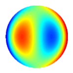 |
|
| (4,2) | Defocus | 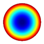 |
|
| (12,4) | Primary Spherical | 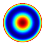 |
|
Table 2.
Results of applying the proposed algorithm to twelve images with different degradation functions.
Table 2.
Results of applying the proposed algorithm to twelve images with different degradation functions.
| # of patterns N/ Aberration type | Aberration Patterns used for Degradation | Degraded Image | |
|---|---|---|---|
|
(a) 1/Defocus |
 |
 |
|
|
(b) 1/ Primary 90° Astigmatism |
 |
 |
|
|
(c) 1/ Secondary Astigmatism |
 |
 |
|
|
(d) 1/ Primary Coma-y |
 |
 |
|
|
(e) 1/ Secondary Coma-x |
 |
 |
|
|
(f) 1/ Primary Spherical |
 |
 |
|
|
(g) 1/ Secondary spherical |
 |
 |
|
|
(h) 2/ defocus and 45°astigmatism |
|
 |
 |
|
(i) 2/ defocus and primary coma-y |
|
 |
 |
|
(j) 2/ Defocus and primary spherical |
|
 |
 |
|
(k) 4/ Defocus, primary 45°astigmatism, coma-y and spherical |
|
 |
 |
|
| |||
|
| |||
|
(L) 4/ Defocus with secondary astigmatism, coma-y, and spherical |
|
 |
 |
|
| |||
|
| |||
Disclaimer/Publisher’s Note: The statements, opinions and data contained in all publications are solely those of the individual author(s) and contributor(s) and not of MDPI and/or the editor(s). MDPI and/or the editor(s) disclaim responsibility for any injury to people or property resulting from any ideas, methods, instructions or products referred to in the content. |
© 2026 by the authors. Licensee MDPI, Basel, Switzerland. This article is an open access article distributed under the terms and conditions of the Creative Commons Attribution (CC BY) license (http://creativecommons.org/licenses/by/4.0/).
Copyright: This open access article is published under a Creative Commons CC BY 4.0 license, which permit the free download, distribution, and reuse, provided that the author and preprint are cited in any reuse.