

Submitted:
07 May 2026
Posted:
08 May 2026
You are already at the latest version
Abstract
Marginal ice zone (MIZ) is a transitional region between dense pack ice and open water. It is a highly dynamic zone under strong interactions between the atmosphere, ocean, sea ice and waves, playing a crucial role in the polar climate and ecosystem. Accurate determination of MIZ is therefore essential for advancing our understanding, modeling and prediction of the polar climate system. In this paper, we introduce and apply a suite of MIZ-related metrics to evaluate the performance of four satellite-derived high-resolution operational sea ice concentration (SIC) products in determination of the MIZs around Svalbard, using the Norwegian ice chart as reference. The metrics used for evaluation include sea ice extent (SIE), MIZ extent (MIZE), length of ice edge (LIE), integrated ice edge error (IIEE), integrated MIZ error (IME), ice edge distance error (IEDE), and MIZ width error (MWE). The evaluation is based on three years of daily SIC data (2023-2025) from four products, including the Bremen AMSR2 SIC data from the University of Bremen (Bremen SIC), the Resolution-enhanced AMSR2 SIC (RE SIC) and Multisensor SIC products (Multisensor SIC) from the Norwegian Meteorological Institute, and the Automated Sea Ice Product (ASIP) from the Copernicus Marine Environment and Monitoring Service (CMEMS) (ASIP SIC). To be consistent with the Norwegian ice chart, the MIZ is defined as MIZ70 and MIZ90, corresponding to SIC thresholds of up to 0.7 and 0.9, respectively. IEDE and MWE are calculated using two types of LIE, the reference LIE (LIEr) from the Norwegian ice chart and the average LIE (LIEa) by averaging the ice chart LIE and the concerned LIE from the four satellite products. The results demonstrate that all four satellite SIC products generally capture the evolution of the sea ice conditions around Svalbard well, but differ in their accuracy when determining the ice edge and MIZs. The Bremen SIC product tends to overlook areas with low SIC, leading to a significant underestimation of SIE and a large IIEE. However, it provides an overall close agreement with the ice chart for the MIZ90 metrics (MIZE, IME and MWE). The RE and ASIP SIC products exhibit strong performance in capturing the ice edge and total SIE, with the ASIP product particularly excelling in accurately representing the ice edge and MIZ70. The Multisensor provides the closest agreement with the ice chart for the IME90, MWE90 and MWEa70, and ranks as the second-best product for the IIEE, IME70 and MWEr70. These results suggest that SAR and Low-frequency AMSR2 channels are especially effective for capturing the lower bounds of the MIZ, while high-frequency channels are more suitable for defining the upper bounds. Despite these strengths, the complex summer surface conditions pose significant challenges for satellite sensors in determining the ice edge and the MIZ, resulting in higher IEDE and MWE values during this period. These results highlight both the capabilities and limitations of satellite-based data in determining the MIZ, particularly under challenging summer conditions. Accurate determination of MIZs may require significant advancements in satellite observation technologies, retrieval algorithms, and more robust methods for integrating multiple sources.
Keywords:
Marginal Ice Zone (MIZ)
; Sea Ice Concentration (SIC)
; Marginal Ice Zone Extent (MIZE)
; Integrated Marginal Ice Zone Error (IME)
; Marginal Ice Zone Width Error (MWE)
; Svalbard
1. Introduction
Marginal ice zone (MIZ) refers to the region of sea ice cover influenced by waves and swell penetrating into the ice from the open ocean [1]. It is a transitional zone between dense pack ice and open water, with the width varying from zero to over hundreds of kilometers. Typical MIZs are found along the southern edges of the Arctic ice pack in the Bering Sea, Greenland Sea, Barents Sea, and Baffin Bay, and along the entire northern edge of the Antarctic sea ice cover [2].
MIZ is a highly dynamic region characterized by strong interactions among the atmosphere, ocean, sea ice and waves. It frequently undergoes intense processes such as rapid sea ice freezing/melting [3,4], mesoscale ocean and atmosphere eddies [5,6], turbulence [7,8], ocean upwelling and downwelling [2,9], therefore playing a crucial role in the polar climate system. Due to the relatively low sea ice concentration (SIC) and sea ice thickness (SIT), the MIZ is also an area much more navigable than the inner dense pack ice, making it an important region for maritime activities [10]. Ocean waves and swell are the primary source of energy for ice breakup in the MIZ and are therefore the key driver determining its properties and extent [11,12,13]. The relatively small ice floes in the MIZ play an important role in shaping the mechanical properties of the ice, affecting its response to winds, ocean waves, and ocean currents [14,15]. These small ice floes have a significant effect on the summer sea ice melting, due to the increased lateral perimeters compared to large ice floes over the same area [16]. Consequently, the MIZ not only modulates local processes but also has far-reaching implications for polar climate, seasonal ice cycle, and the overall ice mass balance in the polar regions.
MIZ is a critical and dynamic region in the polar ocean ecosystems. Extensive phytoplankton blooms, which thrive in the nutrient-rich waters of the MIZ, form the base of the food web and provide a vital food source for a wide variety of species [17]. The MIZ also serves as a crucial habitat for a diverse range of ice-dependent species, such as seals, walruses, and polar bears [18], which use the patchy ice for hunting, breeding, and shelter. Additionally, many seabird species rely on the MIZ for foraging, and Arctic cetaceans like narwhals and belugas use it as a key area for prey and as a refuge from waves. Due to the climate change, changes in the MIZ extent and its physical properties could significantly impact the ecosystems by altering food webs, affecting breeding and hunting grounds for marine mammals, and shifting species distributions [19]. The vital role of MIZ in supporting the diverse species and maintaining the polar ecosystem underscore its importance in the climate-driven transformations, emphasizing the need for continued research and conservation efforts to protect this fragile and essential region.
The sea areas around Svalbard are important for Norwegian marine activities such as shipping, fisheries, tourism, and oil and gas explorations [20]. With the ongoing global warming and retreat of the Arctic sea ice, there has been a remarkable expansion in operational seasons and navigational areas [21]. Sea ice around Svalbard, particularly in the Fram Strait and Barents Sea, presents a major marine hazard and is strongly affected by the atmosphere circulation [22,23], and the northward warm Atlantic Water [24,25]. Consequently, the sea ice conditions in this area are frequently subject to rapid and complex changes, resulting in rapid and significant variations in the MIZ. High-resolution and accurate monitoring and prediction of the MIZ are therefore essential to ensure the safety and efficiency of operations in these regions [26,27]. Numerical experiments show that the skill of MIZ prediction is highly dependent on the quality of the initial MIZ conditions [27], underscoring the critical need for precise and reliable observations of the MIZ.
The extensive spatial coverage of the MIZ and the harsh Arctic environment make in-situ observations of the MIZ both extremely challenging and prohibitively expensive. Therefore remote sensing has become the primary approach for observing the MIZ, based mostly on passive microwave SIC products [28,29,30]. Three high-resolution operational SIC products have been used in the modeling of the atmosphere, ocean and sea ice around Svalbard [27,31,32,33,34]. These include the Advance Microwave Scanning Radiometer 2 (AMSR2) SIC from the University of Bremen (Bremen SIC) [35,36], the resolution-enhanced AMSR2 SIC (RE SIC) [37,38] and the Multisensor SIC [39] from the Norwegian Meteorological Institute. In late 2024, a new high-resolution SIC product, the Automated Sea Ice Product (ASIP) [40], became operational under the Copernicus Marine Environment and Monitoring Service (CMEMS), which covers the whole Arctic.
The main purpose of this study is to evaluate the performance of the above four high-resolution operational SIC products in observing the MIZ around Svalbard, with an aim of identifying the most suitable MIZ product for operational analysis and prediction. Currently two types of MIZ have been defined, namely traditional MIZ and dynamical MIZ [26]. The traditional MIZ is defined solely based on the SIC, whereas the dynamical MIZ considers the impact of waves and can be approximated through a parameterization with combined SIC and SIT [13,26]. Due to the lack of systematic observations of the dynamical MIZ, this study evaluates the MIZ using the traditional MIZ, which has been available in operational ice services for decades. The paper is organized as follows. In Section 2 we describe the used dataset. The evaluation metrics is described in Section 3, and the evaluation results are presented in Section 4. In Section 5, we summarize the main results and discuss the limitations and other relevant issues. The conclusions are given in Section 5.
2. Data
The study area is highlighted by the thick rectangle in Figure 1. It is the model domain of the Barents-2.5km, an operational ocean and sea ice forecast model at the Norwegian Meteorological Institute [31,33,34]. Barents-2.5km has a horizontal grid resolution of 2.5 km and does not include ocean and sea ice information in the Baltic Sea. To keep consistency, we have also excluded the sea ice in the Baltic Sea in this study.
The four high-resolution operational remote sensing SIC products mentioned above are selected for the evaluation of MIZ. The Bremen SIC and RE SIC rely solely on the AMSR2 observations, while the Multisensor SIC and ASIP SIC utilize both AMSR2 and Synthetic Aperture Radar (SAR) observations. In addition to these four operational SIC products, the Norwegian sea charts are used as the reference dataset for evaluation. The used data cover the years 2023-2025. To ensure compatibility across datasets, all the SIC data are interpolated to the Barents-2.5km model grid using the nearest neighbor method.
2.1. Bremen AMSR2 SIC
The version 5.4 of the Bremen AMSR2 SIC (Bremen SIC) is used in this study. It applies the Arctic Radiation and Turbulence Interaction Study (ARTIST) Sea Ice (ASI) algorithm, which primarily relies on the polarization difference of 89 GHz channels [35],
where is brightness temperature, V and H are the vertical and horizontal polarizations. The algorithm uses fixed tie points for 0% () and 100% () SIC, with a standard implementation of for 100% (closed ice) and for 0% (open water). The SIC between open water and 100% ice cover is determined following a third-order polynomial of P. To mitigate the atmospheric influence, the gradient ratios of low-frequency channel pairs are checked against the thresholds [35,36]. Finally, all ASI SICs with corresponding Bootstrap SICs are set to zero [36]. The product is gridded on a polar stereographic grid (EPSG code 3411, Arctic) with a grid resolution of 3.125 km [36]. The uncertainty is calculated following the same procedure as in [35], which sums from three sources: radiometric error from the bright temperature, variability of the tie points, and atmospheric opacity. The standard deviation of the derived SIC is highest in the open water and lowest in the very close drift ice, being about 0.25 when SIC = 0, and about 0.057 when SIC = 1.
2.2. Resolution-Enhanced AMSR2 SIC
The resolution-enhanced AMSR2 SIC (RE SIC) is derived by merging two independent AMSR2 SIC products [37,38], using a simple pan-sharpening method [41]
where and are two SIC products with the algorithms developed in the ESA Climate Change Initiative (CCI) project. Both of them apply a hybrid SIC algorithm to combine two optimized algorithms for low and high SIC conditions [37]. The utilizes three low-frequency channels (19V, 37H and 37V), offering SIC fields with reduced measurement uncertainties but at a coarse spatial resolution. The use measurements solely from the near 90 GHz channels (89H and 89V), providing SIC fields with a higher spatial resolution but increased measurement uncertainties. The resolution enhancement is accomplished by adding the difference between the high-resolution and its blurred component to the coarser resolution (Eq. 2). This RE SIC has high spatial resolution while maintaining relatively low measurement uncertainty [38]. The RE SIC data has two products, daily and sub-daily. The daily data is available from January 2022 until May 2025, whereas the sub-daily data is available since October 2023. For this study, we use the daily data for 2023, and the sub-daily data for 2024 and 2025. A comparison of the daily and sub-daily data for 2024 show small difference, however, the sub-daily data has better temporal coverage.
2.3. Multisensor SIC
The multisensor SIC is generated by merging the AMSR2 SIC and SAR data from Sentinel-1 using the optimal interpolation with a variational analysis approach [39]. The AMSR2 SIC here is the same as the one used for the RE SIC (see Eq. 2). The SAR data used are Sentinel-1 dual-polarized (HH/HV polarization combination) recorded in extra wide swath mode with a swath width of 410 km and a spatial resolution of 93 × 87 m (pixel spacing of 40 × 40 m). The variational analysis is based on techniques commonly used in data assimilation for meteorological models, where the purpose is to minimize a cost-function. The cost-function is formulated as the sum of costs from the different satellite SIC products, along with a contribution from the results of the previous data analysis. The uncertainty of each satellite observation, based on the probability of correct classification of the SAR and AMSR2 data, is used as a weighting of the respective observations during the merging process. The multisensor SIC is daily, with a spatial resolution of 1 km and a polar stereographic projection grid.
2.4. ASIP SIC
The Automated Sea Ice Product (ASIP) within the CMEMS is a high-resolution (1 km), machine-learning-based data product used to map and monitor sea ice in the Arctic and Antarctic, developed primarily by the Danish Meteorological Institute (DMI). This product leverages satellite radar imagery (SAR) to identify SIC, stage of development, and floe sizes on a granular level. The selected Arctic L4 SIC product here is based on the L3 SIC product retrieved from Sentinel-1 and Radarsat Constellation Mission SAR imagery and the AMSR2 data using a deep learning algorithm, gap-filled with OSI SAF EUMETSAT SIC products. ASIP uses all the available frequencies from the AMSR2 sensor (6.9, 7.3, 10.7, 18.7, 23.8, 36.5, 89.0 GHz) in H/V polarization. The automated interpretation of sea ice and water signatures is done using the DMI-ASIP model that has been trained with regional ice charts produced at the DMI Greenland Ice Service and the Canadian Ice Service [40].
2.5. Norwegian Ice Chart
The Norwegian ice chart is produced daily on working days through manual interpretation of satellite data and supplementary observations such as coastal station and ship reports [42]. The charting process integrates diverse satellite observations to obtain an accurate depiction of the sea ice edge and MIZ. Since the ice charting began in 1967, it has undergone significant advancements, incorporating higher spatial resolution and all-weather capable sensors. The primary satellite data used include the weather-independent SAR data from Sentinel-1, RADARSAT-2, and RADARSAT Constellation Mission. In addition, visual and infrared data from METOP, NOAA Advanced Very High Resolution Radiometer (AVHRR), NOAA Visible Infrared Imaging Radiometer Suite (VIIRS), and Sentinel-3 instruments, such as the Ocean and Land Colour Instrument (OLCI) and Sea and Land Surface Temperature Radiometer (SLSTR), are also utilized under cloud-free conditions. These satellites provide multiple daily coverages of the charting area, enabling the production of a scale-free, vectorized ice chart with a nominal resolution of less than 400 m. For the Copernicus Marine Service, a rasterized NetCDF-format version is also produced, resampled to a 1 km grid spacing [43]. This combination of advanced satellite technology and manual interpretation ensures a high-quality, detailed representation of sea ice conditions.
Figure 2 shows a typical winter sea ice condition in the European Arctic. The sea area is divided into seven distinct ice categories: ice-free, open water, very open drift ice, open drift ice, close drift ice, very close drift ice, and fast ice. The corresponding lower and upper bounds for these ice categories are shown in Table 1. It is worth noting that this classification is slightly different from the World Meteorological Organization (WMO) standard classification [1]. For practical applications, the mean value of the lower and upper bounds is employed to represent the SIC for each ice category. In addition, key ice-related parameters such as sea ice extent (SIE) and MIZ are also included in Table 1. The superscripts 70 and 90 represents that the upper bounds of the MIZ are defined as SIC = 0.7 and 0.9, respectively.
3. Evaluation Metrics
3.1. Sea Ice Extent (SIE) and MIZ Extent (MIZE)
SIE is generally defined as the total surface area of the ocean containing the SIC . Similarly, MIZE is commonly defined as the total surface area of the ocean where SIC . However, the numbers for these bounds do not have a clear physical interpretation. To be consistent with the classification used in the Norwegian ice chart (see e.g. Figure 2), we redefine the SIE following [26,44] as
where a denotes SIC. Similarly we define the MIZE as
where the lower bound of 0.1 is consistent with the SIE definition, while the upper bounds are set as for MIZ70 and for MIZ90. These two upper bounds are used to approximate the traditional upper bound of 0.8, which is not employed in the ice categories of the Norwegian ice chart. Such a redefinition provides a clearer physical interpretation. As discussed in [26,44], the lower bound of 0.1 denotes the demarcation between open water and ice (very open drift ice), while the upper bounds of 0.7 and 0.9 correspond to the transitions between open drift ice and close drift ice, and between close drift ice and very close drift ice, respectively. These thresholds reflect distinct physical characteristics: open drift ice is characterized by numerous leads and unconnected ice floes, whereas close drift ice consists primarily of connected floes, which often pose greater risks for navigation. Setting the upper bound at 0.7 for MIZ has practical implications for navigation, as it effectively highlights the regions with lower risks. Furthermore, this threshold is consistent with the WMO definition of pack ice, which is characterized by SIC [1]. This refined approach ensures both practical relevance and consistency with established international standards.
3.2. Length of Ice Edge (LIE)
LIE is calculated following [45], where the ice edge locations are first determined based on the following condition
where are the indices of the 2D gridded SIC, and ∧ is the logical AND operator. The length through an individual edge grid cell is calculated by counting the number, n, of the neighboring edge grid cells (, and ) in the same product [45]
where l is the grid length of the square grid cell, being 2.5 km in the present Barents-2.5km model domain. Thus LIE is the sum over all the edge grid cells
3.3. Integrated Ice Edge Error (IIEE) and Ice Edge Distance Error (IEDE)
The IIEE is determined following [46]
where A denotes the whole model domain, the subscripts f and r denote the estimate (here the four satellite observations) and the reference (here the Norwegian ice chart). In general, the reference dataset should be of high quality for the compared property. The first term on the right side of Eq. (8) denotes the overestimate, and the second term denotes the underestimate. The variable c is determined as following,
Thus an average IEDE can be calculated [45]
where and are the estimated and reference LIEs, respectively. While the IIEE measures the area of mismatch between two fields, the IEDE assesses the mean distance between two ice edges. An alternative estimate of the IEDE is to use the LIEr instead of the average such that
Here and are the average and reference IEDEs.
3.4. Integrated MIZ Error (IME) and MIZ Width Error (MWE)
The definition of IME is similar to the IIEE [44] (see Eq. (8)). The only difference is the definition of the variable c, which is determined as below,
where are the two upper bounds of 0.7 and 0.9 (see Eq. 4). Similar to the IEDE, we introduce MWE to represent the mean width error of IME. Thus we get the average MWE, which is normalized by the average LIEa,
and the reference MWE, which is normalized by LIEr,
4. Results
4.1. Typical Daily MIZ Distribution
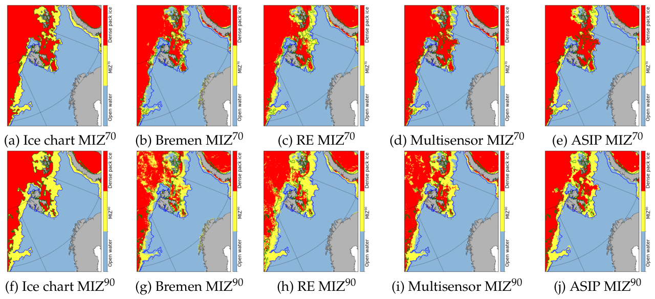
Figure 3 illustrates a typical daily SIC distribution during the winter season, highlighting significant differences between MIZ70 and MIZ90 (cf. Figure 3a and Figure 3f). The total area of MIZ90 is notably larger than that of MIZ70, particularly in the Greenland Sea, Barents Sea and west of Franz Josef Land. The four satellite SIC products generally capture the MIZ characteristics demonstrated by the ice chart, though with varying degrees of accuracy. For instance, the Bremen SIC apparently underestimates the MIZ, both for MIZ70 (Figure 3b vs. Figure 3a) and MIZ90 (Figure 3g vs. Figure 3f), with the most pronounced underestimation in the southern Greenland Sea. By contrast, the RE SIC tends to overestimate the MIZ in both cases of MIZ70 and MIZ90, particularly to the east of Svalbard for the MIZ70 (cf. Figure 3c and Figure 3a), and to the west and north of Svalbard for the MIZ90 (cf. Figure 3h and Figure 3f). The Multisensor and ASIP SIC products exhibits a tendency to underestimate the MIZ, in pariticular to the east of Svalbard and in Fram Strait for the MIZ70 (Figure 3d and Figure 3f vs. Figure 3a), and in the Greenland Sea and Fram Strait for the the MIZ90 (Figure 3i and Figure 3j vs. Figure 3f). In addition, the ASIP SIC apparently underestimates the sea ice along the coast of Novaya Zemlya in both MIZ70 and MIZ90.
The difference between MIZ70 and MIZ90 represents the area of close drift ice, where the SIC ranges from 0.7 to 0.9. Within the extensive regions of dense pack ice, patches of close drift ice are evident in the Bremen and Multisensor products for MIZ90 (Figure 3g and Figure 3i). By contrast, such patches are absent in the ice chart (Figure 3f) and only sporadically present in the RE SIC product (Figure 3h), and rare in the ASIP SIC product. This discrepancy can likely be attributed to the data sources used by these products. The Bremen and Multisensor SIC rely on AMSR2 high-frequency (89 GHz) channels, whereas the RE and ASIP incorporate lower-frequency AMSR2 channels as well as the high-frequency channel data. The exclusive use of AMSR2 high-frequency channels may also contribute to the notable underestimation of the ice edge in the Greenland Sea and east of Franz Josef Land observed in the Bremen product.
4.2. Sea Ice Extent (SIE)
Figure 4a illustrates the calculated SIEs during 2023-2025 for all the observations. While all the satellite products are almost available daily, the Norwegian ice charts are only provided on working days. As a result, there are 742 observations from the Norwegian ice charts after excluding weekends and holidays, which accounts for approximately 68% of the total observations. In addition, some RE SIC observations are excluded due to large area of missing data, thus resulting in a total of 1049 observations. Despite these differences, all the products show a clear seasonal cycle in the SIE, with the largest in early April and the lowest in mid-September (Figure 4a). The SIE mean during 2023-2025 across the four products show small variations, ranging from 10.53 to 11.31. The Bremen SIC product reports the lowest mean SIE (10.53), while the RE SIC product shows the largest mean SIE (11.311).
The SIE variations of the four products are more pronounced during June and October, as more clearly reflected in the the bias analysis (Figure 4b). Unlike the SIE, the SIE bias provides a more consistent evaluation of the SIE levels. The biases indicate that all the satellite products predominantly underestimate the SIE compared to the ice charts, with occasional overestimation observed in the RE and ASIP SIC products. Among the four products, the RE SIC has the smallest bias (-0.17), followed by ASIP (-0.36), whereas the Bremen SIC exhibits the largest bias (-0.89). The greater consistency of the RE and ASIP SIC products with the Norwegian ice charts can be attributed to their utilization of the low-frequency AMSR2 channel data. On the contrary, the tendency of the Bremen SIC product to underestimate SIE is highly likely due to its reliance on the high-frequency AMSR2 channel, as illustrated in Figure 3. The removal of low SIC due to the Bootstrap SIC constraint may also contribute to the underestimation of the Bremen SIE.
4.3. MIZ Extent (MIZE)
The seasonal evolutions of MIZE70 for all the products are shown in Figure 5, together with the biases against the Norwegian ice chart. Compared with the SIE (Figure 4), the MIZE70 demonstrates more pronounced high-frequency temporal variations and less distinct seasonal cycle. On the whole, the Bremen, Multisensor, ASIP and the Norwegian ice chart exhibit consistently low MIZE70 values, ranging from 1.45 to 1.79, whereas the RE product shows comparatively higher values of 2.56. The minimum MIZE70 generally occurs between late September and late October, with a secondary minimum typically observed from late March to early April, although with some fluctuations (Figure 5a). These periods are often coincident with the transitions between refreezing and melting, suggesting the significant influence of thermodynamic processes on the MIZ. This behavior may help explain why satellites and models often achieve higher accuracy in observing and simulating the Arctic sea ice during these periods [44].
As shown in Figure 5a, the RE product reports the largest MIZE70 among the four products during 2023-2025. This results in its largest positive bias relative to the Norwegian ice chart (0.88; Figure 5b). Despite the RE product’s significant overestimation of MIZE70, its SIE agrees best with the ice chart (Figure 4). By contrast, while the Bremen product substantially underestimates the SIE (Figure 4), its MIZE70 is in second alignment with the ice chart. The ASIP MIZE70 shows the closest MIZE70 with the ice chart (Figure 5). In addition, the ASIP biases of MIZE70 and SIE are generally lower than those from the Multisensor product, further suggesting the superior performance of ASIP in capturing SIE and MIZE70.
Figure 6 illustrates the seasonal evolution of the MIZE90 and its associated bias. Similar to MIZE70, the MIZE90 shows high-frequency temporal variations and a less distinct seasonal cycle. The lowest MIZE90 values are observed between late September and late October as the MIZE70. However, unlike the MIZE70, the secondary minimum is less pronounced. It is evident that all the four satellite observations are remarkably overestimated when compared with the ice chart, in particular the RE product (Figure 6a). This discrepancy is particularly apparent in the bias analysis (Figure 6b). Among the products, the Bremen MIZE90 appears to be the closest to the ice chart, with the bias of 0.14, followed by the Multisensor MIZE90, which has the second smallest bias of 0.72. By contrast, both the RE and ASIP products show considerable overestimation, being 2.53 and 1.26 larger than the ice chart, respectively. The MIZE90 values from the four satellite observations are nearly (the Bremen) or more than double (the RE, Multisensor, and ASIP) those of MIZE70, whereas the ice chart MIZE90 is approximately 60% higher than its MIZE70. This indicates that the satellite products generally report more close drift ice than the ice chart.
The absolute biases of MIZE90 are usually significantly larger than those of MIZE70 (Figure 5b vs. Figure 6b), suggesting that the overestimation in MIZE90 primarily arises from the overestimation of close drift ice (SIC: 0.7-0.9). Notably, the biases in the Bremen and Multisensor products shifts from an underestimation in MIZE70 to an overestimation in MIZE90, further highlighting their tendency to overestimate close drift ice. The relatively small bias in the MIZE70 and the much larger bias in the MIZE90 imply that very close drift ice ( SIC: 0.9-1.0) is likely underestimated by the satellite products. This underestimation may be attributed to the misclassification of very close drift ice as close drift ice by the satellite products or to the uncertainties in the ice chart for very close drift ice due to the lack of detailed analysis for very compact ice.
4.4. Length of Ice Edge (LIE)
Figure 7 illustrates the seasonal evolution of the LIE during 2023-2025. The seasonal cycle of ice chart LIE is pronounced (Figure 7a), with a clear minimum occurred repeatedly from late September to early October. From October onward, the LIE increases steadily and remains relatively stable from December to late June, with occasional short-lived spikes in LIE. From July, the LIE generally undergoes a systematic decline until it reaches the annual minimum. On the whole, the minimum and maximum LIEs of the ice chart reach 2004 km and 16473 km, respectively.
All the four satellite products capture the timing of the minimum LIE. Among them, the ASIP closely follows the seasonal variations observed in the ice chart, with a mean LIE of 0.89 km, which is very close to the ice chart mean of 0.85 km. The RE product has the closest mean LIE (0.83 km) to the ice chart, but displays a different seasonal pattern: its LIE values are lower than the ice chart from January to July and higher from July to November. The RE product is relatively stable over the three years, as indicated by its small standard deviation (Figure 7a). This stability, however, results in a large seasonal variation in the RE LIE bias compared to the ice chart (Figure 7b), as also reflected in its higher uncertainty (0.39 km) compared to ASIP’s lower uncertainty (0.20 km). By contrast, the Bremen and Multisensor products consistently overestimate LIE relative to the ice chart, with mean values of 1.34 km and 1.44 km, respectively. These two products closely align with each other, with positive biases of 0.48 km for Bremen and 0.58 km for Multisensor.
4.5. Integrated Ice Edge Error (IIEE) and Ice Edge Distance Error (IEDE)
Figure 8a shows the seasonal evolution of the IIEE for all the four satellite observations against the ice chart. Unlike the bias of LIE, IIEE provides an alternative measure of ice edge error by accounting for spatial mismatches. Among the four products, the Bremen product has the largest IIEE (1.37 km) throughout the period, primarily due to its limitation in detecting regions of low SIC compared to the ice chart (Figure 3). By contrast, the ASIP product has the lowest IIEE (0.71 km), about half of the Bremen IIEE. The Multisensor product records an IIEE of 0.89 km, being the second lowest IIEE. It is noteworthy that both ASIP and Multisensor incorporate SAR observations, which may be the primary reason contributing to their better performance. Their lower IIEEs highlight the advantages of SAR data in enhancing the accuracy of ice edge detection compared to the Bremen and RE.
Figure 8b and Figure 8c illustrate the IEDEa and IEDEr, which represent the IIEE normalized by LIEa and LIEr, respectively. The magnitudes and variations of IEDEa for all four products are less than those of IEDEr as reflected in their respective means and standard deviations. Regardless of the normalization method, the Bremen consistently exhibits the highest IEDE mean (12.91 km for IEDEa; 18.01 km for IEDEr), whereas the ASIP demonstrates the lowest IEDE mean (8.32 km for IEDEa; 8.66 km for IEDEr). Notably, the differences in IEDE between the two normalization approaches are minimal for ASIP and RE, generally less than 1.5 km. This indicates a consist representation of LIE in these two products relative to the ice chart. By contrast, the Bremen and Multisensor products show larger differences in IEDE between the two normalizations methods (3.6 km for Multisensor; 5.1 km for Bremen), indicating less consistency in their alignment with the ice chart.
The ASIP IIEE is noticeably smaller than that of the Multisensor product (Figure 8a). Its IEDEr is also notably smaller than that of Multisensor, resulting in a mean difference of 2.97 km. However, its IEDEa is slightly larger than that of the Multisensor product (Figure 8b). Similarly, while the Bremen IIEE is significantly larger than that of the RE product (Figure 8a), their IEDEa values differ only slightly, with a mean difference of 0.99 km. However, the IEDEr difference between Bremen and RE is much larger, averaging around 4.6 km (Figure 8b). Overall, the evaluation of LIE using IIEE and IEDEr are consistent (cf. Figure 8a and Figure 8c), as all the IIEEs are normalized with the same ice chart LIE.
No pronounced seasonal cycle is observed in the IIEE (Figure 8), which generally exhibits a random distribution over the three years, with minima occurring around early October each year. By contrast, the IEDE shows distinct peaks during the summer seasons, especially for IEDEr. The large variations in IIEEs during other seasons (Figure 8a) are significantly reduced in both IEDEa and IEDEr (Figure 8b and Figure 8c), suggesting a strong correlation between the IIEE and LIE (cf. Figure 7a and Figure 8a).
4.6. Integrated MIZ Error (IME) and MIZ Width Error (MWE)
Figure 9 shows the seasonal evolution of IME70 and MWE70 for all the four satellite observations. Consistent with previous studies [27,44], the IME70 is nearly twice the magnitude of the IIEE. While the overall pattern of IME70 resembles that of the IIEE (cf. Figure 8a and Figure 9a), there are notable differences in the performance of the four satellite products between these metrics. For example, although the Bremen IME70 is nearly identical to the RE IME70, with a mean differences of just 0.01 km, the Bremen IIEE is substantially larger than the RE IIEE, with a mean difference of 0.41 km. Similarly, the Multisensor IME70 is slightly higher than that of ASIP, with a mean difference of 0.17 km, which is consistent with the close alignment of IIEE values, showing a similar mean difference of 0.18 km. Overall, the Multisensor and ASIP products demonstrate significantly lower IME70 compared to Bremen and RE products(Figure 9a), indicating the critical role of SAR observations in improving the accuracy of MIZ detection.
Similar to the IEDEs (Figure 8b and Figure 8c), the variations of MWE70 in the two normalizations are most pronounced during the summer seasons (Figure 9b and Figure 9c), which can be up to 60-110 km. Among the products, RE consistently has the highest MWE in both normalizations, followed by Bremen. By contrast, ASIP and Multisensor have lower MWEs, with ASIP recording the lowest MWEr, and Multisensor reporting the lowest MWEa.
Except for the Bremen product, the other three satellite observations have a doubling of IME when the upper bound of MIZ is increased from 0.7 to 0.9 (Figure 10a vs. Figure 9a), indicating the overall significant overestimation of close drift ice. The mean Bremen IME90 is 2.87 km2, slightly higher than its IME70 value of 2.09 km2. This suggests the Bremen’s classification of close drift ice agrees very well with the ice chart, particularly when compared to the other satellite products. Despite the nearly twofold increase in IME for most products when increasing the upper bound of MIZ, the Multisensor product, similarly to ASIP, has the lowest mean IMZ90 (2.68 km2), while the RE product has the highest mean (3.80 km2) among the four satellite observations.
The seasonal patterns of the MWE90 (Figure 10b and Figure 10c) are similar to those of MWE70 (Figure 9b and Figure 9c), except the amplitudes during the summer seasons are more pronounced in MWE90. In addition, the MWE90 shows another noticeable peak in November 2024. When comparing the MWEs under the two normalization settings, the Multisensor product consistently has the lowest MWEs (24.90 km for ; 35.90 km for for ), while the RE product has the highest MWEs (46.71 km for ; 51.91 km for for ), highlighting the superior performance of Multisensor in representing MIZ90. The mean MWE90s for Bremen (26.51 km for ; 36.50 km for for ) are comparable to those of Multisensor, suggesting that excluding the low-frequency AMSR2 channels tends to improve the determination of the close drift ice.
5. Discussion
5.1. Overall Assessment
In Section 4 we analyzed the metrics of the four satellite SIC products in describing the MIZ around Svalbard, with a primary focus on the seasonal evolution. Here, we summarize these findings and present a statistical overview of the products. Table 2 summarize the key metrics, along with their biases and uncertainties, evaluated against the Norwegian ice charts, a dataset of manual interpretation of satellite data. The best-performance products for each metric is highlighted in bold in Table 2.
The RE and ASIP use both high- and low-frequency AMSR2 channels, providing a close representation of the SIE compared to the ice chart. Due to the missing data in the RE product, the mean RE SIE may be slightly imbalanced compared to the other products. Despite this limitation, the RE product demonstrates a remarkably smaller bias than the others, suggesting that the RE SIE is statistically consistent with the ice chart SIE. By contrast, the Bremen SIC product relies solely on the high-frequency (89 GHz) channels, which has limited capability in capturing areas of low SIC (see e.g. Figure 2). This deficiency results in pronounced underestimation of the SIE and the largest SIE bias among the four products. The Multisensor product, which incorporates the Sentinel-1 SAR observations, shows an improvement in the SIE accuracy. However, its SIE is still underestimated compared to the ice chart, resulting in the second-largest SIE bias among the four products.
The RE and ASIP products demonstrate better consistency with the ice chart in terms of LIE, whereas the Bremen and Multisensor products significantly larger LIEs. This overestimation can primarily be attributed to the spatial resolution of the sensors. The Bremen and Multisensor products rely solely on the high-frequency (89 GHz) AMSR2 channels, while the RE and ASIP products incorporate additional low-frequency AMSR2 channels (e.g. 19 GHz and 37 GHz). The higher resolution observations of the Bremen and Multisensor products can capture more detailed features of the ice edge. This results in a longer measured ice edge due to the fractal effect. It is noted that, while the ASIP SIC has a nominal resolution of 1 km, its actual resolution is much lower. This can be clearly seen from the original ASIP data, where the ice edge is commonly composed of large blocks of equal SIC (not shown). The manually analyzed sea ice chart generally provides a smooth representation of the ice edge, similar to the coarse-resolution observations from the low-frequency AMSR2 channels. As a result, the LIE from the ice chart aligns more closely with the LIEs from the RE and ASIP products. Furthermore, the missing areas of low SIC in the Bremen and Multisensor products also increase the LIE, as can be clearly seen in Figure 2. This is particularly pronounced around the islands of Franz Josef Land and Novaya Zemlya in the 1-km resolution Multisensor product. Finally, the Bremen product often includes fake sea ice along the Norwegian coast, which significantly increases the LIE but only slightly increases the SIE.
The good alignment between the ice chart and the RE and ASIP products leads to a lower bias in the LIE and a smaller IIEE for the RE and ASIP products as shown in Table 2. For IEDE, the ASIP product produces consistently low values in the two methods (IEDEa and IEDEr) . The Multisensor product produces an very lower IEDEa due to its large LIE, but a comparatively higher IEDEr. By contrast, the Bremen product exhibits the highest IEDE values for both IEDEa and IEDEr among the four satellite products. It is worth to note that the IEDEs calculated in this study are based on the daily mean gridded SIC products. These IEDEs could potentially be further reduced when utilizing satellite swath data with closer temporal proximity to the observations.
The ability of the four products to characterize the MIZ was evaluated using metrics of MIZE, MIZE bias, IME and MWE. These metrics were calculated by defining the SIC upper bound as 0.7 or 0.9 to align with the ice chart classification. When the SIC upper bound is set to 0.7, the ASIP product demonstrates superior performance, achieving the closest MIZE to the ice chart, the smallest MIZE bias, and the lowest IME and MWEr. As a result, it stands out as the best performer for representing MIZ70, with an exception of the where the Multisensor product exhibits the lowest error. However, when the upper bound is increased to 0.9, the Bremen product provides a uniformly close agreement with the ice chart, in terms of MIZE, MIZE bias, IME and MWE. The Multisensor and ASIP products performs slightly better than the Bremen product regarding the IME and , but considerably overestimate the MIZE. However, it is difficult to conclude that the Bremen product performs best for the MIZ90, as the ice chart could occasionally overlook detailed classification in the central Arctic [26]. Further studies are needed to clarify this uncertainty.
5.2. Summer IEDE and MWE
Accurate determination of summer MIZs remains a significant challenge due to the limitations of the satellite-based observation system. During the summer melt season, passive (AMSR2 ) and active (SAR) sensors struggle to distinguish between ice and water due to high levels of surface wetness, melt ponds, and atmospheric factors. As a result, errors in sea ice measurements, such as the IEDE and MWE, are significantly larger during the summer months, particularly in August and September, compared to other seasons. These errors can be up to five times larger than those observed in winter (Figure 8, Figure 9 and Figure 10). Furthermore, distinguishing between close drift ice and very close drift ice is particularly challenging, contributing to large IMEs and MWEs, as the LIE during summer is relatively short (Figure 7). The reduction in SIC during summer further exacerbates the problem. The larger areas of low SIC are more likely to be missed due to the limited sensitivity of high-frequency passive microwave radiometers, such as the Bremen and Multisensor products. The limitation of satellite instruments, the complex surface conditions, and seasonal reduction in SIC jointly make accurate measurement of the summer sea ice conditions a significant challenge.
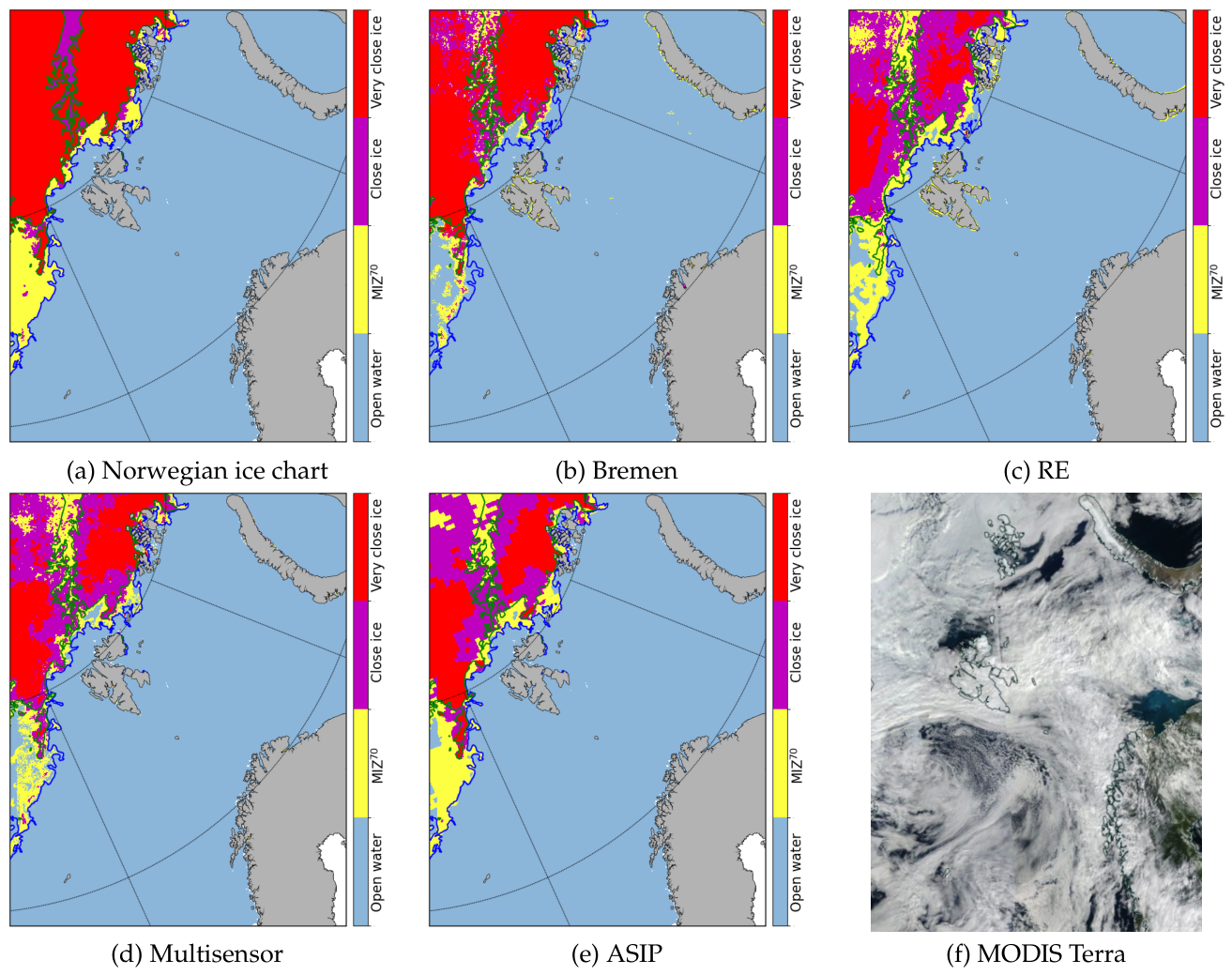
Figure 11 illustrates a representative example of summer sea ice conditions from the four satellite observations together with the Norwegian ice chart. The upper bound of MIZ here is defined as SIC = 0.7, and the close (purple) and very close (red) drift ices are purposely separated. It can be seen that there are notable differences between the satellite products and the manually analyzed ice chart. For instance, the ice chart identifies an elongated patch of close drift ice embedded within very close drift ice. By contrast, the satellite products depict this patch interspersed with varying amounts of MIZ70 or even open water. To the west of this elongated patch, extensive areas of close ice and MIZ70 are observed in the RE, Multisensor and ASIP products, but these features are only sporadically presented in the Bremen product and are completely absent in the ice chart. Similarly, to the east of the elongated patch, large portions of close ice are observed in the RE, Multisensor and ASIP products but are significantly underrepresented by the Bremen product and entirely absent in the ice chart. Another example is observed in the Greenland Sea, where the ice chart classifies the region as a MIZ70 zone (Figure 11b vs. Figure 11a). However, the Bremen product significantly underestimates the extent of this zone, while the RE, Multisensor and ASIP products provide closer but still underestimated representations. These differences highlight the uncertainties and limitations inherent in satellite-derived representations of sea ice conditions during the summer.
Visible and infrared sensors may have higher capability in distinguishing melt pond from open water [47], therefore improving the determination of ice edge as well as the separation between close drift ice and very close drift ice. However, persistent summer cloud cover (e.g. Figure 11f) forbids them for operational use. Manually analyzed ice charts, which incorporate a variety of satellite observations, generally provide more reliable results. However, they also have limitations. For example, small patches of fine-scale features in the central Arctic are often overlooked in the ice charts, as they are less relevant to the Norwegian marine operations. These challenges highlight the need for improving remote sensing techniques to enhance the accuracy of MIZ determination, particularly during the summer season.
5.3. Average LIE vs. Reference LIE
When calculating the IEDE and MWE, two types of LIE are used: the average LIE and the reference LIE, with the latter being derived from the ice chart LIE. As discussed in Section 4.4 and shown in Table 2, these two LIEs can differ substantially. Consequently, the choice of LIE can have a considerable impact on the calculated IEDEs and MWEs (Figure 8, Figure 9 and Figure 10, and Table 2), potentially leading to different conclusions when comparing datasets (Table 2). This raises a question on which LIE is more appropriate for conducting comparisons across multiple datasets.
From the results we can see that the IEDE and MWE calculated using the reference LIE are more consistent with the other metrics, such as IIEE or IME. For example, a smaller IIEE or IME indicates a smaller mismatch relative to the ice chart. When the reference LIE is used, the smaller IIEE or IME is directly translates into a smaller IEDE or MWE. However, this consistency is not guaranteed when the average LIE is used. Moreover, using the reference LIE provides a clear physical interpretation. The IEDE or MWE represents the exact distance or width by which the ice edge deviates from the ice chart ice edge. This direct correspondence makes the reference LIE a more intuitive and meaningful choice for interpreting results. By contrast, when the average LIE is used, it lacks such direct physical connection to the reference dataset, making it less suitable for comprehensive comparisons across datasets.
Given these considerations, the reference LIE is preferable for calculating IEDE and MWE. It ensures consistency with other error metrics, provides a clear physical meaning, and facilitates more reliable and interpretable comparisons across multiple datasets.
6. Conclusions
The Marginal Ice Zone (MIZ) is a dynamic transitional region between dense pack ice and open water, characterized by strong interactions among the atmosphere, ocean, sea ice and waves. This zone plays a critical role in the polar climate system and ecosystem, influencing energy exchanges, ocean circulation, and biological processes in polar regions. Due to the significant contrast between the ocean and sea ice surfaces, even minor deviation in identifying the sea surface can result in substantial errors in the air-sea interactions. Therefore, accurate determination of the MIZ is essential for advancing our understanding, modeling and prediction of the polar climate system, as well as for supporting ecosystem management and climate adaptation strategies in these sensitive regions.
In this study, a comprehensive suit of MIZ-related metrics was introduced and applied to evaluate the effectiveness of four satellite-derived high-resolution operational SIC products — Bremen, RE, Multisensor and ASIP — in determining the MIZs around Svalbard. The Norwegian ice chart was used as the reference dataset. The metrics employed for this evaluation included SIE (Sea Ice Extent), MIZE (MIZ extent ), LIE (Length of ice Edge), IIEE (Integrated Ice Edge Error), IME (Integrated MIZ Error), IEDE (Ice Edge Distance Error), and MWE (MIZ Width Error). To calculate IEDE and MWE, both the reference LIE from the ice chart and the average LIE by averaging a concerned product and the ice chart, were used. Based on the analysis and evaluation of three years of data (2023-2025), we have the following conclusions.
- SAR and Low-frequency AMSR2 channels are effective for determining the sea ice edge, which represents the lower bound of the MIZ. The Bremen product, which solely relies on the high-frequency (89 GHz) AMSR2 channels, tends to overlook the areas with low SIC, leading to larger mismatches in the determination of MIZ from the lower bound. The RE SIC products incorporates low-frequency AMSR2 channels as well as the high-frequency AMSR2 channels, generally performs well in capturing the SIE and LIE. By further incorporation of the SAR measurements, the ASIP achieves highly promising results for the sea ice edge. The Multisensor product merges high-frequency AMSR2 SIC and the Sentinel-1 SAR, producing a better sea ice edge location but worse SIE than the RE when evaluated against the ice chart.
- Although originally trained using the ice charts from the Greenland Ice Service and Canadian Ice Service, the ASIP excels in determining the sea ice edge and MIZ70, where SIC = 0.7 serves as the upper bound for MIZ in the Norwegian ice chart. It exhibits the closest agreement with the Norwegian ice chart across multiple metrics, including LIE, IIEE, IEDE, MIZE70, IME70 and MWE70. By contrast, the other three products generally show less accuracy across these metrics.
- Neglecting low-frequency AMSR2 channels is found to benefit the determination of MIZ90, where SIC = 0.9 is set as the upper bound of the MIZ. The Bremen product exhibits close agreement with the Norwegian ice chart in terms of MIZE90, IME90 and MWE90. The inclusion of the Sentinel-1 SAR in the Multisensor product slightly improves the IME90 and MWE90, but tends to notably degrade the agreement in MIZE. ASIP also performs well in terms of IME90 and MWE90, although it tends to overestimate the MIZE90.
- The reference LIE from the ice chart provides a more intuitive and meaningful basis for interpreting results compared to the average LIE. It offers greater suitability for calculating the IEDE and MWE, ensuring consistency with the reference dataset and enhancing the reliability of the analysis.
- The analysis reveals substantial errors in satellite-based data during the summer months, underscoring the uncertainties and limitations of satellite-derived representations of sea ice conditions during this period. To leverage the strengths and mitigate the limitations of individual satellite product, merging existing SIC dataset presents a promising solution. For instance, previous studies ([48]) successfully merged the the Special Sensor Microwave Imager/Sounder (SSMIS) and AMSR2 data with the Norwegian ice chart, significantly reducing uncertainties at the ice edge and in the coastal areas. Similarly, Wang et al. [26] combined AMSR2 SIC with the Norwegian ice chart, and further integrated daily SMOS SIT with weekly CS2SMOS SIT, resulting in fused products that provided consistent descriptions of sea ice edge and MIZ. These approaches demonstrate the potential of data merging and fusion to enhance the accuracy and reliability of MIZ assessments, paving the way for more robust monitoring and modeling of polar sea ice dynamics.
Author Contributions
Conceptualization, K.W. and C.W; methodology, K.W; software, K.W.; validation, K.W. and C.W.; formal analysis, K.W. and C.W.; investigation, K.W. and C.W.; resources, K.W.; data curation, K.W.; writing—original draft preparation, K.W.; writing—review and editing, C.W and K.W.; visualization, K.W.; project administration, K.W.; funding acquisition, K.W. All authors have read and agreed to the published version of the manuscript.
Funding
This research received funding from the Norwegian Research Council through project 4SICE (grant no. 328886), the Norwegian FRAM Flagship program through project SUDARCO (grant no. 551323), and the European Union’s Horizon Europe research and innovation programme through project EU-INTERCHANGE (grant No. 101181585).
Institutional Review Board Statement
Not applicable.
Informed Consent Statement
Not applicable.
Data Availability Statement
The AMSR2 data is available at https://data.seaice.uni-bremen.de/amsr2/. The ASIP data is available at https://thredds.met.no/thredds/myocean/SIW-TAC/siw-dmi-arc-hires-sic.html. The Multisensor data is available at https://thredds.met.no/thredds/myocean/SIW-TAC/siw-metno-arc-hires-sict.html. The Norwegian sea ice chart data is available at https://thredds.met.no/thredds/myocean/SIW-TAC/siw-metno-svalbard.html. The MODIS image is from https://worldview.earthdata.nasa.gov/.
Acknowledgments
The authors are grateful to Gunnar Spreen in the University of Bremen for the discussions on the AMSR2 data, and to Till Rasmussen in the Danish Meteorological Institute for the discussions on the ASIP data. We gratefully thank our colleagues Frode Dinessen for the explanations of the Multisensor data, Josef Rusin and Atle Sørensen for providing the Resolution-enhanced data, and Arne Melsom and Nick Hughes for the discussions on the ice edge length and ice edge distance error.
Conflicts of Interest
The authors declare no conflicts of interest. The funders had no role in the design of the study; in the collection, analyses, or interpretation of data; in the writing of the manuscript; or in the decision to publish the results.
Abbreviations
The following abbreviations are used in this manuscript:
| AMSR2 | Advance Microwave Scanning Radiometer 2 |
| ARTIST | Arctic Radiation and Turbulence Interaction Study |
| ASI | ARTIST Sea Ice |
| ASIP | Automatic Sea Ice Product |
| AVHRR | Advanced Very High Resolution Radiometer |
| CCI | Climate Change Initiative |
| CMEMS | Copernicus Marine Environment and Monitoring Service |
| CS2SMOS | CryoSate-2 and SMOS |
| IEDE | Ice Edge Distance Error |
| IIEE | Integrated Ice Edge Error |
| IME | Integrated Marginal Ice Zone Error |
| LIE | Length of Ice Edge |
| MIZ | Marginal Ice Zone |
| MIZE | Marginal Ice Zone Extent |
| MODIS | Moderate Resolution Imaging Spectroradiometer |
| MWE | Marginal Ice Zone Width Error |
| OLCI | Ocean and Land Colour Instrument |
| RE | Resolution Enhanced |
| SAR | Synthetic Aperture Radar |
| SIC | Sea Ice Concentration |
| SIE | Sea Ice Extent |
| SIT | Sea Ice Thickness |
| SLSTR | Sea and Land Surface Temperature Radiometer |
| SSMIS | Special Sensor Microwave Imager/Sounder |
| VIIRS | Visible Infrared Imaging Radiometer Suite |
References
- WMO. Number No. 259; SEA ICE NOMENCLATURE. WMO, 2014.
- Røed, L.P.; O’Brien. A coupled ice-ocean model of upwelling in the marginal ice zone. J. Geophys. Res. 1983, 88, 2863–2872. [Google Scholar] [CrossRef]
- Josberger, E.G. Sea ice melting in the marginal ice zone. J. Geophys. Res.-Ocean. 1983, 88, 2841–2844. [Google Scholar] [CrossRef]
- Tucker, W.B.; Grenfell, T.C.; Onstott, R.G.; Perovich, D.K.; Gow, A.J.; Shuchman, R.A.; Sutherland, L.L. Microwave and physical properties of sea ice in the winter marginal ice zone. J. Geophys. Res. 1991, 96, 4573–4587. [Google Scholar] [CrossRef]
- Johannessen, J.A.; Johannessen, O.M.; Svendsen, E.; Shuchman, R.; Manley, T.; Campbell, W.J.; Josberger, E.G.; Sandven, S.; Gascard, J.C.; Olaussen, T.; et al. Mesoscale eddies in the Fram Strait marginal ice zone during the 1983 and 1984 Marginal Ice Zone Experiments. J. Geophys. Res.-Ocean. 1987, 92, 6754–6772. [Google Scholar] [CrossRef]
- Inoue, J.; Hori, M.E. Arctic cyclogenesis at the marginal ice zone: A contributory mechanism for the temperature amplification? Geophys. Res. Lett. 2011, 38. [Google Scholar] [CrossRef]
- Padman, L.; Dillon, T.M. Turbulent mixing near the Yermak Plateau during the Coordinated Eastern Arctic Experiment. J. Geophys. Res. 1991, 96, 4769–4782. [Google Scholar] [CrossRef]
- Sunfjord, A.; Fer, I.; Kasajima, Y.; Svendsen, H. Observations of turbulent mixing and hydrography in the marginal ice zone of the Barents Sea. J. Geophys. Res.-Ocean. 2007, 112. [Google Scholar] [CrossRef]
- Häkkinen, S. Coupled ice-ocean dynamics in the marginal ice zones: Upwelling/downwelling and eddy generation. J. Geophys. Res. 1986, 91, 819–832. [Google Scholar] [CrossRef]
- Stephenson, S.R.; Smith, L.C.; Agnew, J.A. Divergent long-term trajectories of human access to the Arctic. Nat. Clim. Change 2011, 1, 156–160. [Google Scholar] [CrossRef]
- Squire, V.A.; Dugan, J.P.; Wadhams, P.; J., R.P.; K., L.A. Of ocean waves and sea-ice. Annu. Rev. Fluid Mech. 1995, 27, 115–168. [Google Scholar] [CrossRef]
- Squire, V.A. Of ocean waves and sea-ice revisited. Cold Reg. Sci. Tech. 2007, 49, 110–133. [Google Scholar] [CrossRef]
- Dumont, D.; Kohout, A.; L., B. A wave-based model for the marginal ice zone including a floe breaking parameterization. J. Geophys. Res.-Ocean. 2011, 116. [Google Scholar] [CrossRef]
- Shen, H.H.; Hiber, W.D.; Lepparanta, M. The role of floe collisions in sea ice rheology. J. Geophys. Res.-Ocean. 1987, 92, 7085–7096. [Google Scholar] [CrossRef]
- Feltham, D.L. Granular flow in the marginal ice zone. Phil. Trans. R. Soc. A 2005, 363, 1677–1700. [Google Scholar] [CrossRef]
- Steele, M. Sea ice melting and floe geometry in a simple ice-ocean model. J. Geophys. Res.-Ocean. 1992, 97, 17729–17738. [Google Scholar] [CrossRef]
- Falk-Petersen, S.; Haakon, H.; Budgell, W.P.; Hegseth, E.N.; Korsnes, R.; Løyning, T.B.; Ørbæk, J.B.; Kawamura, T.; Shirasawa, K. Physical and ecological processes in the marginal ice zone of the northern Barents Sea during the summer melt period. J. Mar. Syst. 2000. [Google Scholar] [CrossRef]
- Hamilton, C.D.; Kovacs, K.M.; Ims, R.A.; Aars, J.; Strøm, H.; Lydersen, C. Spatial overlap among an Arctic predator, prey and scavenger in the marginal ice zone. Mar. Ecol. Prog. Ser. 2017, 573, 45–59. [Google Scholar] [CrossRef]
- Derocher, A.E.D.; Lunn, N.I.J.; A., S.I. Polar Bears in a Warming Climate. Integr. Comp. Biol. 2004, 44, 163–176. [Google Scholar] [CrossRef]
- Olsen, J.; Hovelsrud, G.; Kaltenborn. Increasing Shipping in the Arctic and Local Communities’ Engagement: A Case from Longyearbyen on Svalbard. In Arctic Marine Sustainability; Pongrácz, E., Pavlov, V., Hänninen, N., Eds.; Springer, 2020; pp. 305–331. [Google Scholar] [CrossRef]
- Stocker, A.; Renner, A.; Knol-Kauffman, M. Sea ice variability and maritime activity around Svalbard in the period 2012–2019. Sci. Rep. 2020, 10, 17043. [Google Scholar] [CrossRef]
- Vinje, T. Fram Strait ice flux and atmospheric circulation: 1950-2000. J. Clim. 2001, 14, 3508–3517. [Google Scholar] [CrossRef]
- Maslanik, J.; Drobot, S.; Fowler, C.; Emery, W.; Barry, R. On the Arctic climate paradox and the continuing role of atmospheric circulation in affecting sea ice conditions. Geophys. Res. Lett. 2012, 34, 1501–1515. [Google Scholar] [CrossRef]
- Sandø, A.; Nilsen, J.; Gao, Y.; Lohmann, K. Importance of heat transport and local air-sea heat fluxes for Barents Sea climate variability. J. Geophys. Res.-Ocean. 2010, 115, C07013. [Google Scholar] [CrossRef]
- Smedsrud, L.; Esau, I.; Ingvaldsen, R.; Eldevik, T.; Haugan, P.; Li, C.; V., L.; Olsen, A.; Omar, A.; Otterå, O.; et al. The role of the Barents Sea in the Arctic climate system. Rev. Geophys. 2013, 51, 415–449. [Google Scholar] [CrossRef]
- Wang, K.; Wang, C.; Dinessen, F.; Spreen, G.; Ricker, R.; X., T.K. Multisensor data fusion of operational sea ice observations. Front. Mar. Sci. 2024, 11, 1366002. [Google Scholar] [CrossRef]
- Wang, K.; Wang, C.; Hughes, N.; Ali, A. Improving short-term forecasts of sea ice edge and marginal ice zone around Svalbard. Front. Mar. Sci. 2025, 12, 1588769. [Google Scholar] [CrossRef]
- Strong, C. Atmospheric influence on Arctic marginal ice zone position and width in the Atlantic sector, February–April 1979–2010. Clim. Dyn. 2012, 39, 3091–3102. [Google Scholar] [CrossRef]
- Rolph1, R.J.; Feltham, D.L.; Schröder, D. Changes of the Arctic marginal ice zone during the satellite era. The Cryosphere 2020, 14, 1971–1984. [Google Scholar] [CrossRef]
- Song, L.; Zhao, X.; Wu, Y.; Gong, J.; Li, B. Assessing Arctic marginal ice zone dynamics from 1979 to 2023: insights into long-term variability and morphological changes. Environ. Res. Lett. 2025, 20, 034032. [Google Scholar] [CrossRef]
- Duarte, P.; Brændshøi, J.; Shcherbin, D.; Barras, P.; Albretsen, J.; Gusdal, Y.; Szapiro, N.; Martinsen, A.; Samuelsen, A.; Wang, K.; et al. Implementation and evaluation of open boundary conditions for sea ice in a regional coupled ocean (ROMS) and sea ice (CICE) modeling system. Geosci. Model Dev. 2022, 15, 4373–4392. [Google Scholar] [CrossRef]
- Müller, M.; Batrak, Y.; Dinessen, F.; Grote, R.; Wang, K. Challenges in the Description of Sea Ice for a Kilometer-Scale Weather Forecasting System. Weather Forecast. 2023, 38, 1157–1171. [Google Scholar] [CrossRef]
- Röhrs, J.; Gusdal, Y.; Rikardsen, E.; Duran Moro, M.; Brændshøi, J.; Kristensen, N.M.; Fritzner, S.; Wang, K.; Sperrevik, A.K.; Idžanović, M.; et al. Barents-2.5km v2.0: An operational data-assimilative coupled ocean and sea ice ensemble prediction model for the Barents Sea and Svalbard. Geosci. Model Dev. 2023, 16, 5401–5426. [Google Scholar] [CrossRef]
- Durán Moro, M.; Sperrevik, A.K.; Lavergne, T.; Bertino, L.; Gusdal, Y.; Iversen, S.C.; Rusin, J. Assimilation of satellite swaths versus daily means of sea ice concentration in a regional coupled ocean–sea ice model. The Cryoshpere 2024, 18, 1597–1619. [Google Scholar] [CrossRef]
- Spreen, G.; Kaleschke, L.; Heygster, G. Sea ice remote sensing using AMSR-E 89-GHz channels. J. Geophys. Res. Ocean. 2008, 113, C02S03. [Google Scholar] [CrossRef]
- Melsheimer, C. ASI Version 5 Sea Ice Concentration User Guide, Version V0.92; Unversity of Bremen, 2019; p. 10 pp. [Google Scholar]
- Lavergne, T.; Sørensen, A.; Tonboe, R.; Pedersen, L. CCI+ sea ice ECV sea ice concentration algorithm theoretical basis document; accessed; European Space Agency, 2021; p. 41 pp. (accessed on in April 2026)Technical report. [Google Scholar]
- Rusin, J.; Lavergne, T.; Doulgeris, A.P.; Scott, K.A. Resolution enhanced sea ice concentration: a new algorithm applied to AMSR2 microwave radiometry data. Ann. Glaciol. 2024, 8, 1–12. [Google Scholar] [CrossRef]
- Dinessen, F.; Korosov, A.; Wettre, C.; Lavergne, T.; Kreiner, M. Arctic Sea Ice Concentration, Arctic Sea Ice Type, Greenland Sea ice concentration, SEAICE_ARC_PHY_AUTO_L4_NRT_011_015, Issue: 1.2. MERCATOR OCEAN, Technical report. Toulouse, France, 2024. [Google Scholar]
- Wulf, T.; Buus-Hinkler, J.; Singha, S.; Shi, H.; Kreiner, M.B. Pan-Arctic sea ice concentration from SAR and passive microwave. The Cryophere 2024, 18, 5277–5300. [Google Scholar] [CrossRef]
- Meng, X.; Shen, H.; Li, H.; Zhang, L.; Fu, R. Review of the pan-sharpening methods for remote sensing images based on the idea of meta-analysis: Practical discussion and challenges. Inform. Fusion 2019, 46, 102–113. [Google Scholar] [CrossRef]
- Copeland, W.; Wagner, P.; Hughes, N.; Everett, A.; Robertsen, T. The MET Norway Ice Service: a comprehensive review of the historical and future evolution, ice chart creation, and end user interaction within METAREA XIX. Front. Mar. Sci. 2024, 11, 1400479. [Google Scholar] [CrossRef]
- Dinessen, F.; Hackett, B. Product user manual for regional high resolution sea ice charts Svalbard region; Copernicus Marine Service, 2018; p. 16 pp. [Google Scholar]
- Wang, K.; Ali, A.; Wang, C. Local analytical optimal nudging for assimilating AMSR2 sea ice concentration in a high-resolution pan-Arctic coupled ocean (HYCOM 2.2.98) and sea ice (CICE 5.1.2) model. The Cryosphere 2023, 17, 4487–4510. [Google Scholar] [CrossRef]
- Melsom1, A.; Palerme, C.; Müller, M. Validation metrics for ice edge position forecasts. Ocean Sci. 2019, 15, 615–630. [Google Scholar] [CrossRef]
- Goessling, H.F.; Tietsche, S.; Day, J.J.; Hawkins, E.; Jung, T. Predictability of the Arctic sea ice edge. Geophys. Res. Lett. 2016, 43, 1642–1650. [Google Scholar] [CrossRef]
- Rösel, A.; Kaleschke, L.; Birnbaum, G. Melt ponds on Arctic sea ice determined from MODIS satellite data using an artificial neural network. The Cryosphere 2012, 6, 431–446. [Google Scholar] [CrossRef]
- Wang, K.; Lavergne, T.; Dinessen, F. Multisensor data merging of sea ice concentration and thickness. Adv. Polar Sci. 2020, 31, 1–13. [Google Scholar] [CrossRef]
Figure 1.
Study area: Barents-2.5km model domain shown by the thick rectangle. The grid numbers of the domain are 739 × 949, with the grid length of 2.5 km.
Figure 1.
Study area: Barents-2.5km model domain shown by the thick rectangle. The grid numbers of the domain are 739 × 949, with the grid length of 2.5 km.
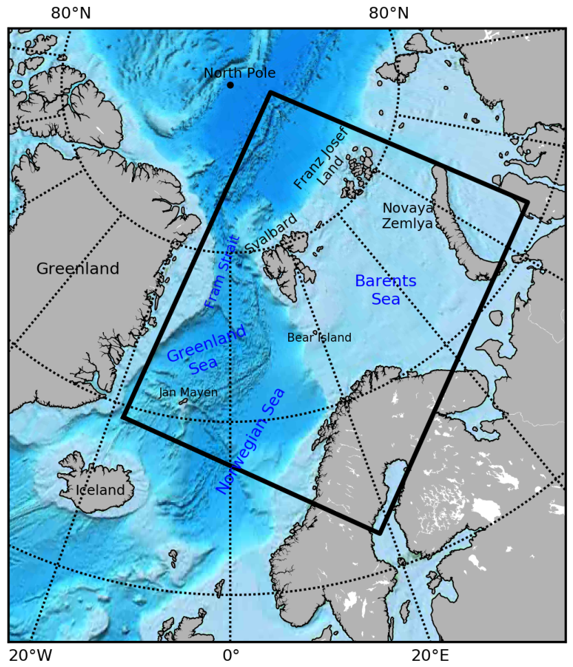
Figure 2.
A typical Norwegian ice chart showing winter sea ice conditions in the European Arctic. The black lines show the areas with available satellite images from Sentinel-1 or RadarSat-2. The red lines show the sea surface temperature.
Figure 2.
A typical Norwegian ice chart showing winter sea ice conditions in the European Arctic. The black lines show the areas with available satellite images from Sentinel-1 or RadarSat-2. The red lines show the sea surface temperature.
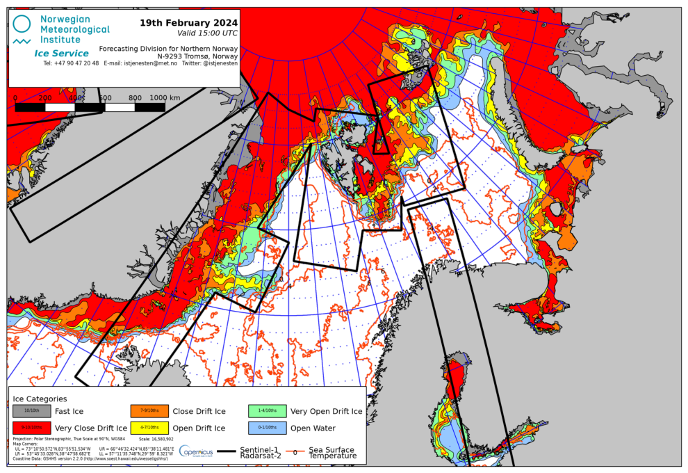
Figure 3.
Daily SIC distributions from observations (Ice chart, Bremen, RE, Multisensor and ASIP) with MIZ70 (a-e) and MIZ90 (f-j) on 19 February 2025. The ice cover is separated into dense pack ice (red), MIZ (yellow) and open water (light blue). The blue lines show the SIE of the ice chart, and the green lines show the demarcation between MIZ and dense pack ice of the ice chart.
Figure 3.
Daily SIC distributions from observations (Ice chart, Bremen, RE, Multisensor and ASIP) with MIZ70 (a-e) and MIZ90 (f-j) on 19 February 2025. The ice cover is separated into dense pack ice (red), MIZ (yellow) and open water (light blue). The blue lines show the SIE of the ice chart, and the green lines show the demarcation between MIZ and dense pack ice of the ice chart.
| (a) Ice chart MIZ70 | (b) Bremen MIZ70 | (c) RE MIZ70 | (d) Multisensor MIZ70 | (e) ASIP MIZ70 |
| (f) Ice chart MIZ90 | (g) Bremen MIZ90 | (h) RE MIZ90 | (i) Multisensor MIZ90 | (j) ASIP MIZ90 |
Figure 4.
Seasonal evolution of the SIEs in the Barents-2.5km domain during 2023-2025: a) SIE, and b) Bias of SIE. The biases of the SIE are calculated via the satellite observations (Bremen, RF, Multisensor and ASIP) - Ice chart.
Figure 4.
Seasonal evolution of the SIEs in the Barents-2.5km domain during 2023-2025: a) SIE, and b) Bias of SIE. The biases of the SIE are calculated via the satellite observations (Bremen, RF, Multisensor and ASIP) - Ice chart.
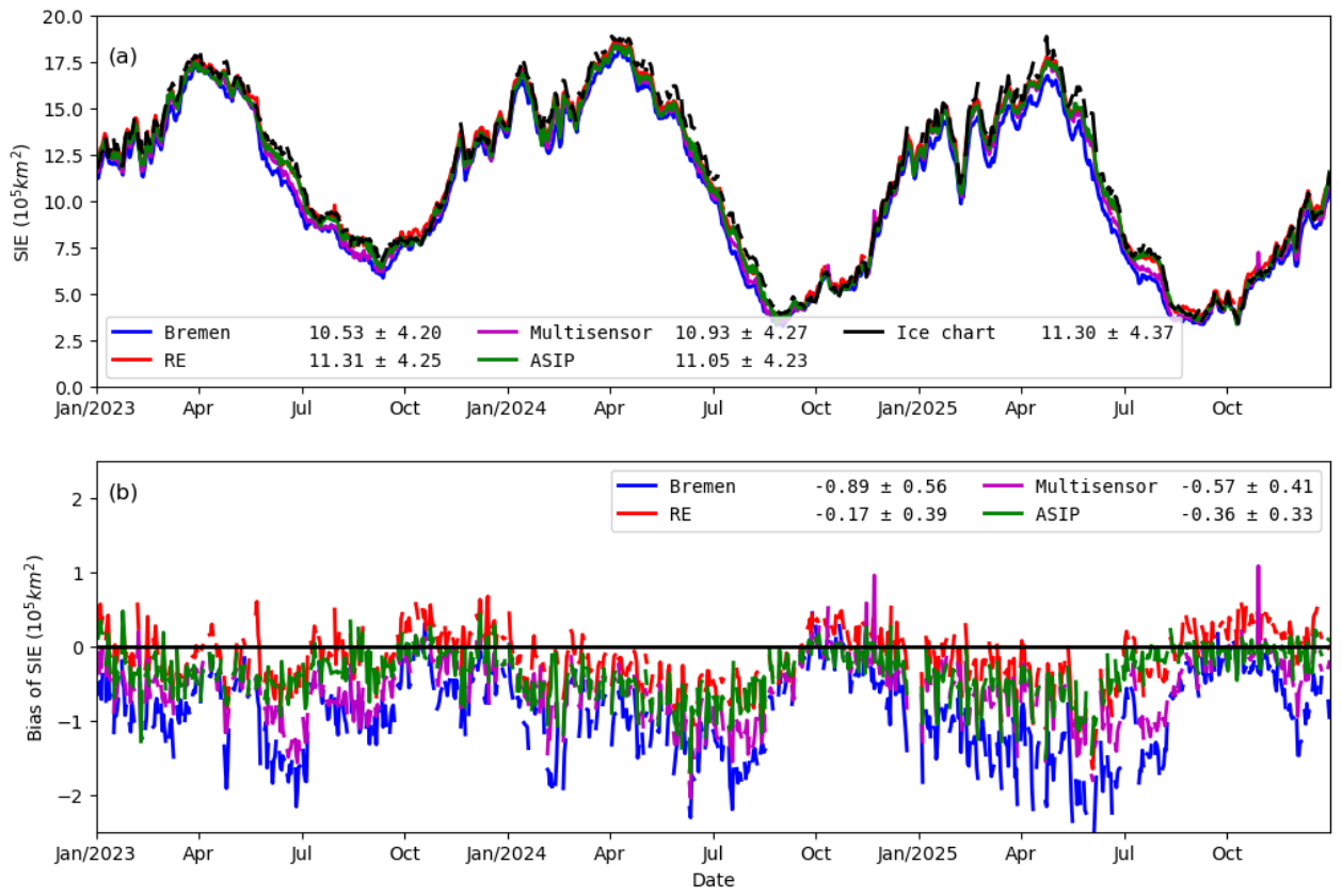
Figure 5.
Seasonal evolution of the MIZE70s in the Barents-2.5km domain during 2023-2025: a) MIZE70, and b) Bias of MIZE70. The biases are calculated via the satellite observations (Bremen, RF, Multisensor and ASIP) - Ice chart.
Figure 5.
Seasonal evolution of the MIZE70s in the Barents-2.5km domain during 2023-2025: a) MIZE70, and b) Bias of MIZE70. The biases are calculated via the satellite observations (Bremen, RF, Multisensor and ASIP) - Ice chart.
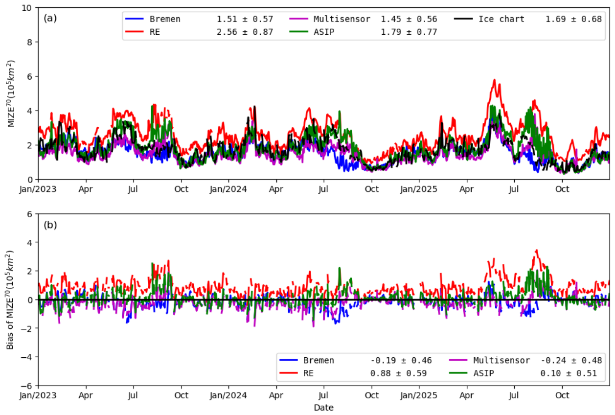
Figure 6.
Seasonal evolution of the MIZE90s in the Barents-2.5km domain during 2023-2025: a) MIZE90, and b) Bias of MIZE90. The biases are calculated via the satellite observations (Bremen, RF, Multisensor and ASIP) - Ice chart.
Figure 6.
Seasonal evolution of the MIZE90s in the Barents-2.5km domain during 2023-2025: a) MIZE90, and b) Bias of MIZE90. The biases are calculated via the satellite observations (Bremen, RF, Multisensor and ASIP) - Ice chart.
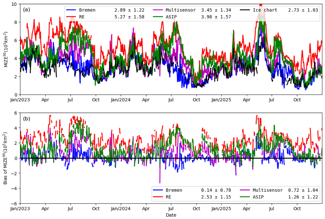
Figure 7.
Seasonal evolution of the LIE in the Barents-2.5km domain during 2023-2025: a) LIE, and b) Bias of LIE. The biases are calculated via the satellite observations (Bremen, RF, Multisensor and ASIP) - Ice chart.
Figure 7.
Seasonal evolution of the LIE in the Barents-2.5km domain during 2023-2025: a) LIE, and b) Bias of LIE. The biases are calculated via the satellite observations (Bremen, RF, Multisensor and ASIP) - Ice chart.
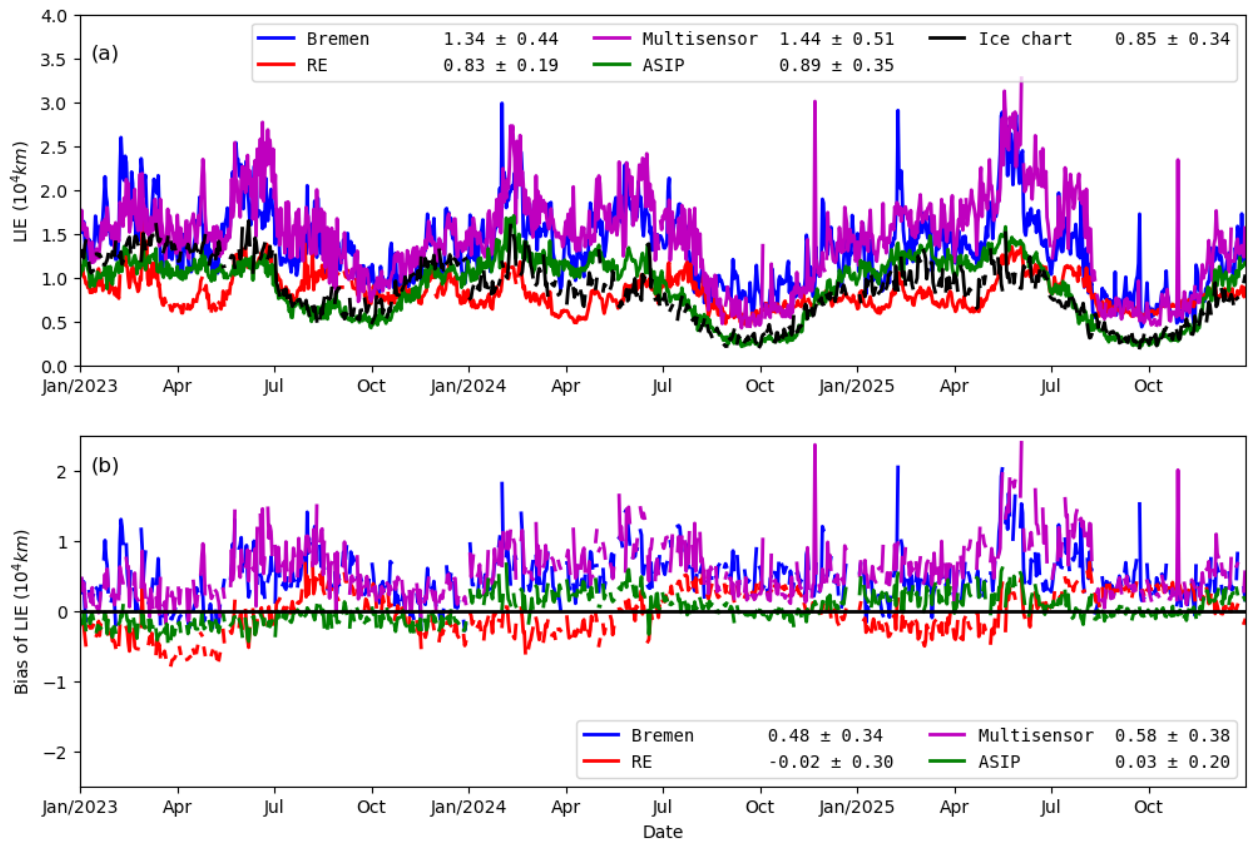
Figure 8.
Seasonal evolution of the ice edge errors in the Barents-2.5km domain during 2023-2025: a) IIEE, and b) IEDEa, the IIEE normalized by the average LIE, and c) IEDEr, the IIEE normalized by the reference LIE.
Figure 8.
Seasonal evolution of the ice edge errors in the Barents-2.5km domain during 2023-2025: a) IIEE, and b) IEDEa, the IIEE normalized by the average LIE, and c) IEDEr, the IIEE normalized by the reference LIE.
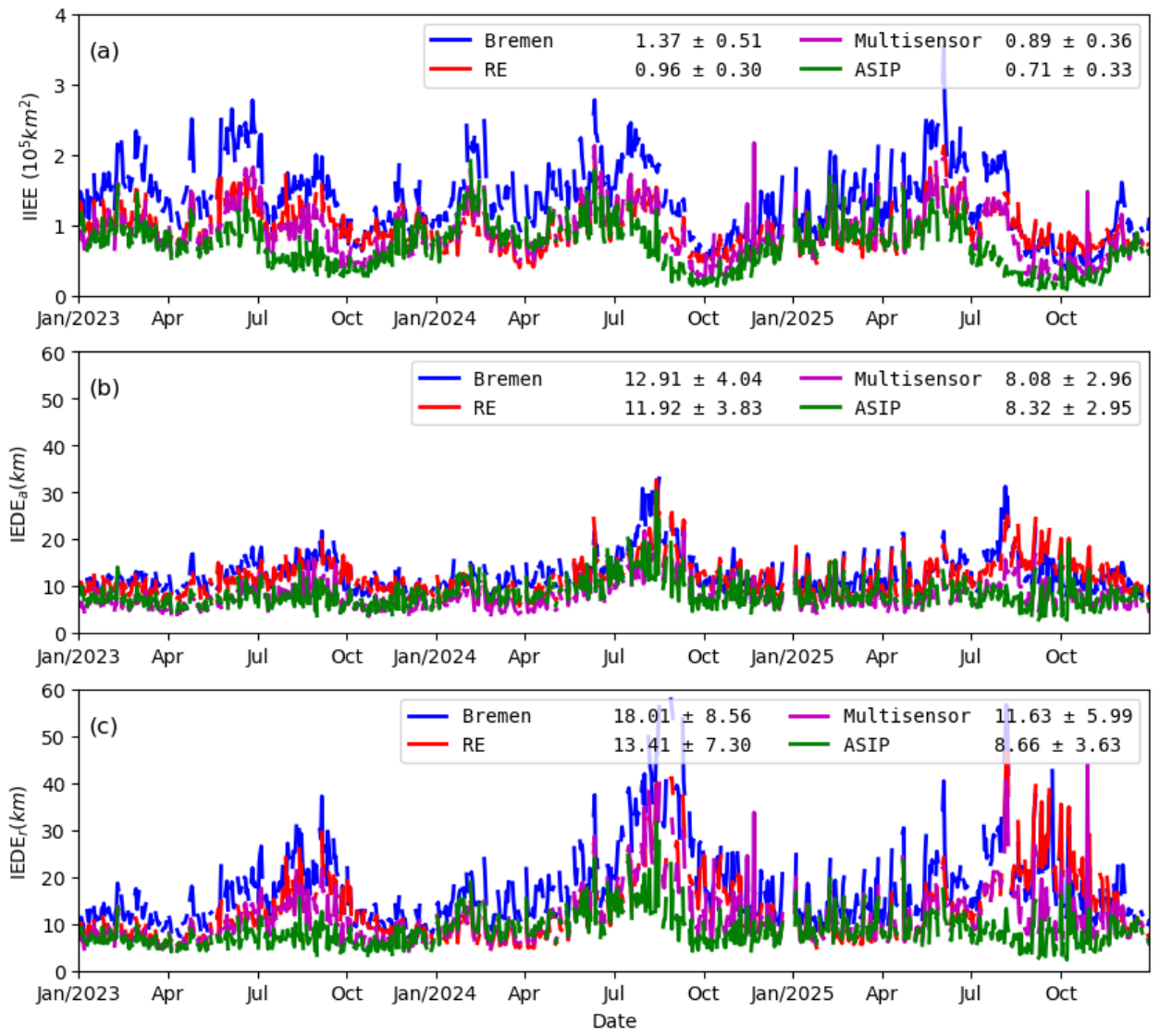
Figure 9.
Seasonal evolution of the MIZ70 errors in the Barents-2.5km domain during 2023-2025: a) IME70, and b) , the IME70 normalized by the average LIE, and c) , the IME70 normalized by the reference ice chart LIE.
Figure 9.
Seasonal evolution of the MIZ70 errors in the Barents-2.5km domain during 2023-2025: a) IME70, and b) , the IME70 normalized by the average LIE, and c) , the IME70 normalized by the reference ice chart LIE.
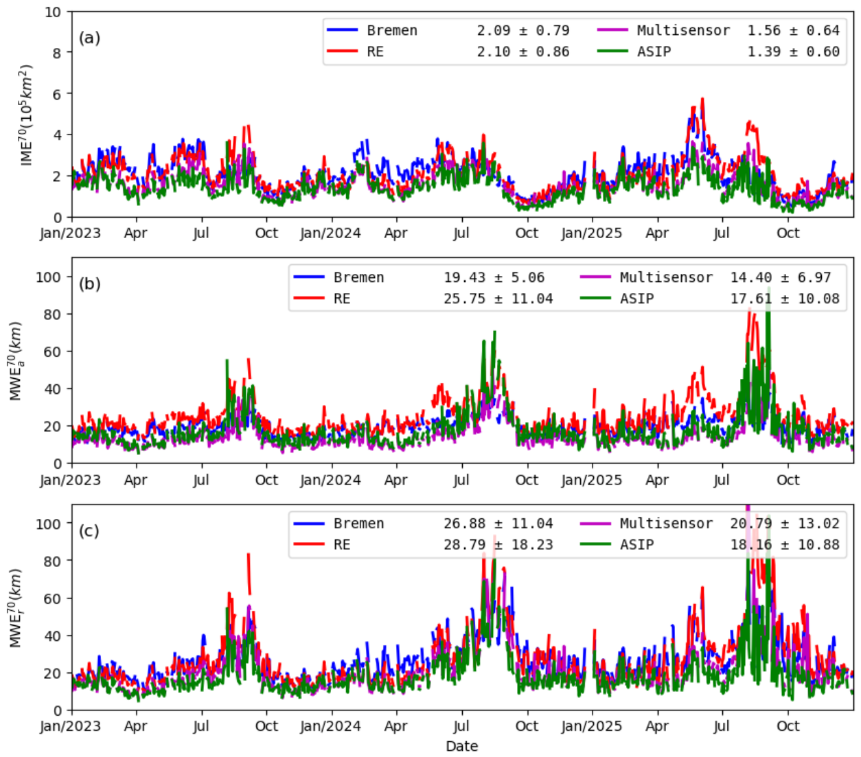
Figure 10.
Seasonal evolution of the MIZ90 errors in the Barents-2.5km domain during 2023-2025: a) IME, and b) MWE normalized with the average LIE, and c) MWE normalized with the ice chart LIE.
Figure 10.
Seasonal evolution of the MIZ90 errors in the Barents-2.5km domain during 2023-2025: a) IME, and b) MWE normalized with the average LIE, and c) MWE normalized with the ice chart LIE.
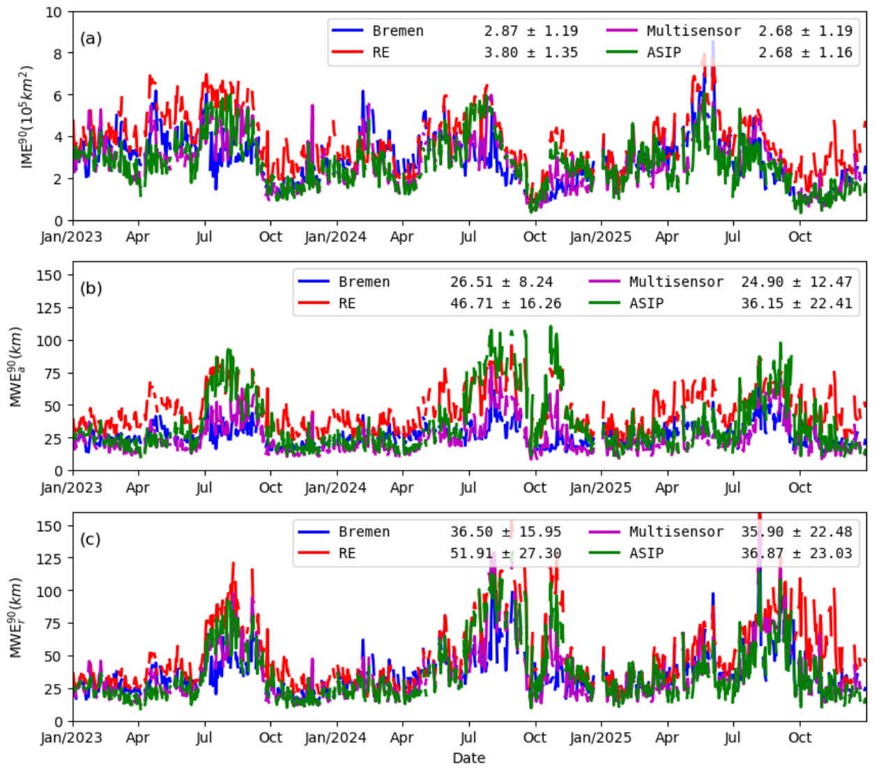
Figure 11.
Daily sea ice conditions on 15 August 2023 from (a) Norwegian ice chart, (b) Bremen, (c) RE, (d) Multisensor, (e) ASIP, and (f) MODIS Terra. The ice conditions are separated into open water (light blue), MIZ70 (yellow), close drift ice and very close drift ice in (a-e). The blue and green lines represent the SIC equal to 0.1 and 0.9 in the Norwegian ice chart, respectively. The MODIS Terra is a true color image for the same region.
Figure 11.
Daily sea ice conditions on 15 August 2023 from (a) Norwegian ice chart, (b) Bremen, (c) RE, (d) Multisensor, (e) ASIP, and (f) MODIS Terra. The ice conditions are separated into open water (light blue), MIZ70 (yellow), close drift ice and very close drift ice in (a-e). The blue and green lines represent the SIC equal to 0.1 and 0.9 in the Norwegian ice chart, respectively. The MODIS Terra is a true color image for the same region.
| (a) Norwegian ice chart | (b) Bremen | (c) RE |
| (d) Multisensor | (e) ASIP | (f) MODIS Terra |

Table 1.
Typical sea ice categories based on ice concentration together with common ice features defined by the Norwegian ice chart. SIE denotes sea ice extent, and MIZ70 and MIZ90 represent the MIZ with the upper bounds of SIC at and , respectively.
Table 1.
Typical sea ice categories based on ice concentration together with common ice features defined by the Norwegian ice chart. SIE denotes sea ice extent, and MIZ70 and MIZ90 represent the MIZ with the upper bounds of SIC at and , respectively.
| ice category | lower bound | upper bound |
|---|---|---|
| ice free | 0.0 | 0.0 |
| open water | 0.0 | 0.1 |
| very open drift ice | 0.1 | 0.4 |
| open drift ice | 0.4 | 0.7 |
| close drift ice | 0.7 | 0.9 |
| very close drift ice | 0.9 | 1.0 |
| fast ice | 1.0 | 1.0 |
| SIE | 0.1 | 1.0 |
| 0.1 | 0.7 | |
| 0.1 | 0.9 |
Table 2.
Summary of the four satellite SIC observations in describing the MIZs around Svalbard during 2023-2025. The highlighted (dark black) numbers show the highest scores for the corresponding metrics. The superscripts 70 and 90 represent the upper bound being 0.7 and 90 for the defined MIZ, respectively. The subscripts a and r represent the average LIE and ice chart LIE being used for normalization, respectively.
Table 2.
Summary of the four satellite SIC observations in describing the MIZs around Svalbard during 2023-2025. The highlighted (dark black) numbers show the highest scores for the corresponding metrics. The superscripts 70 and 90 represent the upper bound being 0.7 and 90 for the defined MIZ, respectively. The subscripts a and r represent the average LIE and ice chart LIE being used for normalization, respectively.
| Satellite SIC products | ||||||
|---|---|---|---|---|---|---|
| Metrics | unit | Bremen | RE | Multisensor | ASIP | Ice chart |
| SIE | 105 km2 | 10.53±4.20 | 11.31±4.25 | 10.93±4.27 | 11.05±4.23 | 11.30±4.37 |
| SIE bias | 105 km2 | -0.89±0.56 | -0.17±0.39 | -0.57±0.41 | -0.36±0.33 | |
| LIE | 104 km | 1.34±0.44 | 0.83±0.19 | 1.44±0.51 | 0.89±0.35 | 0.85±0.34 |
| LIE bias | 104 km | 0.48±0.34 | -0.02±0.30 | 0.58±0.38 | -0.03±0.20 | |
| IIEE | 105 km2 | 1.37±0.51 | 0.96±0.30 | 0.89±0.36 | 0.71±0.33 | |
| IEDEa | km | 12.91±4.04 | 11.92±3.83 | 8.08±2.96 | 8.32±2.95 | |
| IEDEr | km | 18.01±8.56 | 13.41±7.30 | 11.63±5.99 | 8.66±3.63 | |
| MIZE70 | 105 km2 | 1.51±0.57 | 2.56±0.87 | 1.45±0.56 | 1.79±0.77 | 1.69±0.68 |
| MIZE70 bias | 105 km2 | -0.19±0.46 | 0.88±0.59 | -0.24±0.48 | 0.10±0.51 | |
| IME70 | 105 km2 | 2.09±0.79 | 2.10±0.86 | 1.56±0.64 | 1.39±0.60 | |
| km | 19.43±5.06 | 25.75±11.04 | 14.40±6.97 | 17.61±10.08 | ||
| km | 26.88±11.04 | 28.79±18.23 | 20.79±13.02 | 18.16±10.88 | ||
| MIZE90 | 105 km2 | 2.89±1.22 | 5.27±1.50 | 3.45±1.34 | 3.98±1.57 | 2.73±1.03 |
| MIZE90 bias | 105 km2 | 0.14±0.78 | 2.53±1.15 | 0.72±1.04 | 1.26±1.22 | |
| IME90 | 105 km2 | 2.87±1.19 | 3.80±1.35 | 2.68±1.19 | 2.68±1.16 | |
| km | 26.51±8.24 | 46.71±16.26 | 24.90±12.47 | 36.15±22.41 | ||
| km | 36.50±15.95 | 51.91±27.30 | 35.90±22.48 | 36.87±23.03 | ||
Disclaimer/Publisher’s Note: The statements, opinions and data contained in all publications are solely those of the individual author(s) and contributor(s) and not of MDPI and/or the editor(s). MDPI and/or the editor(s) disclaim responsibility for any injury to people or property resulting from any ideas, methods, instructions or products referred to in the content. |
© 2026 by the authors. Licensee MDPI, Basel, Switzerland. This article is an open access article distributed under the terms and conditions of the Creative Commons Attribution (CC BY) license.
Copyright: This open access article is published under a Creative Commons CC BY 4.0 license, which permit the free download, distribution, and reuse, provided that the author and preprint are cited in any reuse.