

Submitted:
06 May 2026
Posted:
07 May 2026
You are already at the latest version
Abstract
This paper focuses on the optimization of engineering decision-making under uncertain environments. Engineering decision-making requires optimizing the input of production materials and the selection of equipment and processes under the constraints of cost and expected return to minimize costs and maximize production benefits. As an efficient formal verification technique, model checking provides a new approach to solve this problem. Traditional model checking mainly focuses on qualitative verification, while quantitative model checking techniques (such as probabilistic and possibilistic model checking) have been developed gradually, among which possibilistic model checking is more suitable for systems with fuzzy uncertainty. However, existing possibilistic model checking techniques have obvious defects: first, they only target closed systems and do not consider the interaction between the system and the external environment; second, the simple information aggregation method leads to information desynchronization and information loss; third, they cannot model and verify systems with incomplete information. Model checking technology based on possibilistic decision processes considers uncertain action selection and initially solves the problem of modeling and verification of open systems. The author has introduced the idea of quality constraints into possibilistic temporal logic to solve the problems of information desynchronization and information loss in possibilistic model checking; moreover, the author has established the theories of Intuitionistic Fuzzy Kripke Structure (IFKS) and Intuitionistic Fuzzy Computation Tree Logic (IFCTL), which can model and verify systems with incomplete information. To improve the usability and accuracy of engineering decisions, this paper will draw on the ideas and methods of uncertain selection of decision behaviors, quality constraints, and incompleteness modeling, extend IFKS to Weighted Intuitionistic Fuzzy Kripke Structure (WIFKS), induce IFCTL to Intuitionistic Fuzzy Decision Tree Logic (IFDTL), propose an algorithm for solving IFDTL model checking problems, and present a solution algorithm for multi-attribute engineering decision-making based on IFDTL model checking, along with its correctness proof and complexity analysis. Finally, a case study of Qinling health-preserving tourism planning is given to verify the rationality and efficiency of the proposed method, providing a new formal solution for uncertain engineering decision-making.
Keywords:
quality
; intuitionistic fuzzy
; temporal logic
; model checking
; engineering decision-making
MSC: 68T37
1. Introduction
The engineering decision-making problem of optimizing the input of production materials and the selection of production equipment and processes at each stage under realistic constraints to minimize the comprehensive cost and maximize the production benefit has long been a research focus. As a formal automatic verification technology, model checking has been successfully applied in the correctness analysis of computer software and hardware design, communication protocols, security protocols and other fields since it was proposed by Clarke, Emerson et al. in 1981 [1,2]. An important application of model checking in engineering decision-making is to model the engineering implementation process, describe the engineering property constraints with temporal logic formulas, and solve the decision schemes that meet the engineering constraints through model checking technology.
Traditional model checking technology mainly verifies the qualitative properties of the system, while in recent years, scholars have paid more attention to the verification of quantitative properties of the system and proposed quantitative model checking technology. This technology includes probabilistic model checking [3,4,5,6] and possibilistic model checking [7,8,9,10,11,12,13,14,15,16,17]. Probabilistic model checking is used to verify the properties of the system with deterministic probability distribution in state transition, while possibilistic model checking is used to verify the properties of the system with fuzzy uncertainty in state transition, which has stronger expressiveness than probabilistic model checking.
Some scholars have introduced quality constraints and corresponding information fusion operators into the possibilistic linear temporal logic (PoLTL) and possibilistic computation tree logic (POCTL), proposing the quality-constrained fuzzy linear temporal logic (QFLTL) [18] and quality-constrained fuzzy computation tree logic (QFCTL) [19], and studied their model checking problems, which solves the defects of unsynchronized fusion of temporal property truth values and path reachability, information loss, and inability to reflect the importance of system properties in the aggregation of subformula satisfaction values in traditional possibilistic temporal logic.
In addition, relevant scholars have extended the possibilistic model checking technology, extended the generalized possibility Kripke structure (GPKS) to the possibility decision process (PDP), and established the possibility decision theory, which effectively solves the modeling and decision-making problems of fuzzy systems with non-deterministic action selection in state transition [20,21,22]. The intuitionistic fuzzy set [23], as an extension of the fuzzy set [24], can more objectively and naturally represent the uncertain membership and non-membership relationships between objects. Based on this, the intuitionistic fuzzy Kripke structure (IFKS), intuitionistic fuzzy computation tree logic (IFCTL) and their equivalence with possibilistic computation tree logic (PoCTL) and classical computation tree logic (CTL) have been established, providing a more accurate modeling method for uncertain systems [25].
Considering the complexity of engineering decision-making factors and the uncertainty and incompleteness of system parameters, to improve the usability and accuracy of engineering decisions, this study intends to extend the intuitionistic fuzzy Kripke structure (IFKS) to the weighted intuitionistic fuzzy Kripke structure (WIFKS), and derive the intuitionistic fuzzy decision tree logic (IFDTL) from IFCTL. We will study the intuitionistic fuzzy expected measure and multi-attribute engineering decision-making problem based on this, formally describe the single-attribute and multi-attribute engineering decision-making problems, propose the corresponding solution algorithm based on IFDTL model checking, prove the correctness of the algorithm, and analyze its complexity. Finally, a case study of Qinling health-preserving tourism planning is given to verify the rationality and efficiency of the proposed method, providing a reliable formal solution for engineering decision-making under uncertain environments.
Table 1 lists the differences and relationships among existing possibilistic temporal logics and their model checking. In this table, we use model names to denote the sets of models they construct, and use temporal logic names to denote their formula sets. Thus, the set inclusion relations reflect the expressive power of models or temporal logics. For brevity, we use TL to denote both LTL and CTL; for instance, PoTL denotes PoLTL and PoCTL. References [8,9] have proved that KS⊂PKS and TLPoTL. References [10,11] have shown that PKSGPKS and PoTLGPoTL. References [18,19] verified that GPoTLQFTL. References [20,21] demonstrated that GPKSPDP. References [25,26] proved that GPKSIFKS and GPoTLIFTL.
This paper proposes WIFKS, IFDTL, and the corresponding model-checking techniques, and verifies that IFKSWIFKS and IFCTLIFDTL, which further confirms that the proposed IFDTL and its model-checking approach are theoretically and practically significant.
2. Weighted Intuitionistic Fuzzy Kripke Structure
Intuitionistic fuzzy measures and intuitionistic fuzzy Kripke structures serve as the fundamental models for intuitionistic fuzzy model checking. Their definitions are reviewed as follows.
Definition 1 [Intuitionistic Fuzzy Measure] [25] Let be a non-empty set, be a collection consisting of some subsets of , and denote the intuitionistic fuzzy unit interval. If is closed under the operations of countable union and complementation, then is called a -algebra. An intuitionistic fuzzy possibility measure on the -algebra is a mapping : , which satisfies the following conditions:
(1) ;
(2) ;
(3) If ,,then,If a mapping only satisfies conditions (1) and (3) above, then it is called a generalized intuitionistic fuzzy measure.
(1)
is a countable, non-empty set of states;
(2)
is an intuitionistic fuzzy transition distribution function;
(3) I is an intuitionistic fuzzy distribution function for initial states;
(4)
is a countable, non-empty set of atomic propositions;
(5) L
is a labeling function. For any
and
,
denotes the intuitionistic fuzzy satisfaction value of the atomic proposition p at state
.
If
and
are finite, then M is called a finite intuitionistic fuzzy Kripke structure.
In an IFKS , a path is defined as an infinite sequence of states, denoted by , where . The mapping L is an intuitionistic fuzzy function that assigns a set of intuitionistic fuzzy atomic propositions to each state. For any and , represents the atomic proposition at state . For notational simplicity, is abbreviated to . The expression denotes the suffix path starting from state . Letbe the set of all infinite paths in ; for any state,
denotes the set of all infinite paths starting from
. We define
as the set of all directly reachable states from
.
We next present the definition of the intuitionistic fuzzy measure over an IFKS.
Definition 3 [25] Let be an intuitionistic fuzzy Kripke structure (IFKS). A mapping is defined as follows:
where
. For any
, we define:
,
In this way, the mapping
is called an intuitionistic fuzzy measure on
.
Costs or benefits in engineering decision-making (typically non-negative rational numbers
) are treated as weights assigned to the transition relations or states in an intuitionistic fuzzy Kripke structure, from which a Weighted Intuitionistic Fuzzy Kripke Structure (WIFKS) is induced.
Definition 4 [WIFKS] A Weighted Intuitionistic Fuzzy Kripke Structure (WIFKS)is a 2-tuple , where:
(1) is an intuitionistic fuzzy Kripke structure (IFKS);
(2)
is a set of weight functions, with
, denoting the number of decision attributes. For any
, the weight function
assigns a specific cost or benefit
to each transition relation
.
Naturally, the cumulative weight for a finite path
is defined as follows:
Remark 1 It should be noted that a WIFKS may be associated with multiple weight functionsin practical engineering decision-making scenarios; the definition ofpresented herein is merely a general abstract form. Suppose a specific decision-making problem involvesdecision attributes (costs or benefits), denoted by the decision attribute set . The scale of the weight functions is then given by .
3. Formal Description of Optimal Engineering Decision-Making
Engineering decision schemes are characterized by paths in an IFKS, the feasibility of a scheme is quantified by the intuitionistic fuzzy measure of its corresponding path, and the cost or benefit of a scheme is represented by the weight functions of the IFKS. The objective function for intuitionistic fuzzy attribute decision-making needs to integrate two facets of information: the cost (or benefit) of a decision scheme (i.e., a path) and the feasibility of the decision scheme (i.e., the intuitionistic fuzzy measure of the path). We next present the definition of the weighted composition operation for intuitionistic fuzzy numbers to formalize this information fusion approach.
Definition 5 For an arbitrary intuitionistic fuzzy numberand an arbitrary non-negative rational number , the weighted composition operations for intuitionistic fuzzy numbers are defined as follows:
(1) Cost-weighted composition operation: ;
(2) Benefit-weighted composition operation: .
We next discuss the closure property of the weighted composition operations for intuitionistic fuzzy numbers.
Proposition 1 The weighted composition operationsandfor intuitionistic fuzzy numbers are closed operations on.
Proof: Let an arbitrary non-negative rational number and an arbitrary intuitionistic fuzzy number be given. Since, the operation is closed on . Similarly, we have , which implies that the operation is also closed on .
We next discuss the rationality of the weighted composition operations for intuitionistic fuzzy numbers.
Proposition 2 For any with , and any intuitionistic fuzzy number , the following conclusions hold:
(1)
;
(2)
.
Proof: Let be arbitrary with , and take any . We first prove the following lemma:
Define the function ; its derivative is . Since , we have , and thus conclusion (1) holds.
Define the function ; its derivative is . Since , we have , and thus conclusion (3) holds. It then follows that for an arbitrary intuitionistic fuzzy number :
Based on the definition of the order relation for intuitionistic fuzzy numbers in reference [27], the conclusions of Proposition 2 are thus established.The conclusions of Proposition 2 characterize the following fact: for the same decision scheme (with a fixed intuitionistic fuzzy number , the cost-weighted composition operation is adopted for cost calculation, where a lower cost yields a larger objective function value; the benefit-weighted composition operation is adopted for benefit calculation, where a higher benefit leads to a larger objective function value. The cumulative weight of a path and the intuitionistic fuzzy measure of the path can be synthesized via the weighted composition operations for intuitionistic fuzzy numbers, and the resulting value serves as the fundamental basis for engineering decision-making.
Proposition 3 For any and any intuitionistic fuzzy numbers and , if , then the following conclusions hold:
(1) ;
(2) .
Proof: Following the proof procedure of Proposition 2, we define the functions and , both of which are monotonically increasing on the interval [0,1] . In light of the definition of the order relation for intuitionistic fuzzy numbers in reference [24], the conclusions of Proposition 3 can be readily proven.Propositions 1, 2 and 3 fully demonstrate that the weighted composition operations for intuitionistic fuzzy numbers defined in Definition 5 are well-defined. Multiple costs and benefits can be regarded as multiple attributes that influence engineering decision-making. In engineering management and decision-making, the factors to be considered include time cost (project duration), financial cost, human resource cost, expected social benefits, economic benefits, and the intuitionistic fuzzy possibility of completing each engineering step under the constraints of specific attributes. We now explore how to solve the multi-attribute decision-making problem based on the WIFKS model. Since the calculation of intuitionistic fuzzy measures is primarily path-based, it is optimal for one engineering decision scheme to correspond to a single path in practical applications.
In the WIFKS model, the set of finite paths that satisfy certain property constraints (e.g., completing the project within a specified cost range or a desired benefit threshold) is defined as the satisfiable decision scheme set, denoted by , where . We next present the formal description of the single-attribute and multi-attribute optimal decision-making problems on .
The basic idea of single-attribute decision-making is as follows:
(1) For cost-type attributes: among all schemes with the same cost (where schemes are in one-to-one correspondence with paths in the WIFKS), select the maximum intuitionistic fuzzy measure (i.e., path reachability) of the feasible schemes, and perform the cost-weighted composition operation () on this maximum measure and the corresponding cost. The minimum value from the resulting set of composite scores is defined as the cost expectation of the cost attribute, and the set of paths corresponding to this minimum value constitutes the optimal decision scheme set for the attribute.
(2) For benefit-type attributes: among all schemes with the same benefit, select the maximum intuitionistic fuzzy measure (path reachability) of the feasible schemes, and perform the benefit-weighted composition operation () on this maximum measure and the corresponding benefit. The maximum value from the resulting set of composite scores is defined as the benefit expectation of the benefit attribute, and the set of paths corresponding to this maximum value forms the optimal decision scheme set for the attribute.
Definition 6 (Single-Attribute Decision-Making) Let be a WIFKS and an intuitionistic fuzzy measure function. Given a finite path set with , the relevant concepts of single-attribute decision-making on are defined as follows:
(1) Cost Expectation on Π for Cost-type Attributes:
(2) Expected Path Set in for Cost-type Attributes:
;
(3) Benefit Expectation on for Benefit-type Attributes:
(4) Expected Path Set in for Benefit-type Attributes:
Since the membership degree and non-membership degree both take values in the interval [0,1] while the weight is generally a large value, the result of tends to (1,0) and that of tends to (0,1) . This impairs the comparison and selection of optimal alternatives. Thus, the intuitionistic fuzzy measures of decision schemes can be normalized to the interval [0,1] to avoid such issues and facilitate comparison. For any , the normalized weight of π is defined as follows:
We then simply replace with in Definition 6.
For multi-attribute decision-making, it is necessary to integrate all cost and benefit information to derive a comprehensive evaluation score for each scheme. The set of paths with the highest scores is then selected as the optimal decision scheme. We next present the formal description of WIFKS-based multi-attribute decision-making.
Definition 7 [Multi-Attribute Decision-Making] Let be a WIFKS, an intuitionistic fuzzy measure function, and a finite path set be given with . Let the decision attribute set be denoted by. The relevant concepts of intuitionistic fuzzy multi-attribute decision-making on are defined as follows:
(1) Preference weight set: , where . In particular, if there is no preference for the weights of decision attributes, ;
(2) For any , let label the index of in ; for any with , let denote the cumulative weight of path with respect to attribute . Let be the set of cumulative weights of all finite paths in with respect to . The normalized weight corresponding to is defined as:
If
is a cost-type attribute:
If
is a benefit-type attribute:
(3) Multi-attribute decision-making score set: . The multi-attribute decision-making score for is defined as:
(4) Multi-attribute optimal decision-making score function: ;
(5) Multi-attribute optimal decision scheme function: .
Both cost and benefit weights are normalized to the unit interval [0,1] via Eqs. (7) and (8), and a larger normalized weight corresponds to a lower cost (or a higher benefit) for the attribute. Accordingly, in Eq. (9), we first take the product of the attribute preference weight and the normalized weight , then synthesize the preference-weighted sum with the intuitionistic fuzzy measure of the decision scheme using the benefit-weighted composition operator . This definition is natural and consistent with the decision-making logic.
4. Intuitionistic Fuzzy Decision Tree Temporal Logic
The prerequisite for solving the multi-attribute decision-making problem above is the identification of the satisfiable decision scheme set , where must satisfy constraints of temporal properties. We now introduce attribute decision operators into IFCTL to propose the Intuitionistic Fuzzy Decision Tree Temporal Logic (IFDTL) for constraining decision schemes, and further characterize the logical properties of IFDTL. We first present the syntax and semantics of IFDTL.
4.1. Syntax and Semantics of IFDTL
Definition 8 [The Syntax of IFDTL] The syntax of IFDTL is defined as follows:
State Formulas of IFDTL:
whereis a path formula,,are state formulas,,denotes the weight constraint predicate for thedecision attribute, andis the set of weight constraint predicates fordecision attributes.is single-attribute satisfiable decision scheme operator.is multi-attribute satisfiable decision scheme operator.is single-attribute decision expected score operator.is single-attribute decision expected scheme operator.multi-attribute optimal score operator.is multi-attribute optimal decision scheme operator.
Path Formulas of IFDTL:
Where are state formulas and .
To characterize the semantics of IFDTL in a concise manner, we first introduce the concept of the decision core for IFDTL path formulas.
Defination 9 [Decision Core for IFDTL Path Formulas]For anyany, and any IFDTL state formulas, suppose there exists a path fragmentwithandthat satisfies the following conditions:
(1) For all }, if , then ;
(2) For all , ;
(3) (4) For all , .
Then is called the decision core of the IFDTL formula on path , denoted by .
If there exists no that satisfies the above four conditions simultaneously, the IFDTL formula is said to have no decision core (or an empty decision core) on path , denoted by .
If the constraint is additionally imposed on the above four conditions, then is called the bounded decision core of the IFDTL formula on path , denoted by .
Remark 2Let . All states on appear on the path π, but they do not need to be consecutive on . In fact, the constraints above ensure two aspects simultaneously: on the one hand, they guarantee that (by Conditions 3 and 4); on the other hand, they eliminate cycles on (by Conditions 1 and 2). This constraint intuitively characterizes the achievement of the decision objective () in a shortest and most efficient manner. Precisely because the decision core is the "shortest and most efficient" path to reach the decision objective, it is unique.
Definition 10 [Semantics of IFDTL] Let be a WIFKS, an intuitionistic fuzzy measure function, and the decision attribute set. For any, any , and any , the semantics of IFDTL is recursively defined as follows:
(1) ;
(2) ;
(3) ;
(4) ;
(5) ;
(6) ;
(7) ;
(8) ;
(9) ;
(10) ;
(11) ;
(12) .
where Exp denotes the cost-type or benefit-type attribute expectation function defined in Definition 6, and denotes the cost-type or benefit-type attribute expected path function defined in Definition 6. is the multi-attribute optimal decision-making score function defined in Definition 7, and is the multi-attribute optimal decision scheme function defined in Definition 7.
We next present the semantics of several important IFDTL formulas that do not appear in the IFDTL syntax but can be reduced to the syntactically defined formulas:
(13) ;
(14) ;
(15) ;
(16) .
Remark 3The semantics of IFDTL differs significantly from that of other computation tree temporal logics. An important task of IFDTL semantics is to compute the path sets that satisfy temporal property constraints or weight predicate constraints. Thus, the computational results of the IFDTL operators and ☐ defined in Definition 10 are paths or path sets.
4.2. Logical Properties of IFDTL
For the sake of descriptive convenience, an IFDTL formula is used to denote the path, path set, or satisfaction value derived from its semantic computation. We next investigate the logical properties of IFDTL formulas.
Theorem 1[Finiteness Principle] Let be a WIFKS, and let be IFDTL state formulas. The following conclusions hold:
(1) ;
(2) .
Proof: (1) For any and any , we need to prove . Let ; it is necessary and sufficient to prove . We now proceed by contradiction: suppose . By Condition (4), for all , which implies for all. Since , the sequence contains at least distinct states by Condition (1) of Definition 9. As has at most states in total, it follows that for all . This further implies , which violates Condition (3) of Definition 9. This contradiction arises from the assumption , so the assumption is false and must hold.
(2) Since (where “" denotes the tautology), Conclusion (2) of Theorem 1 holds naturally.□
Theorem 1 indicates that for any , any , and any given IFDTL state formulas and , the length of is bounded by (i.e., ). Starting from the initial state , perform a breadth-first search (BFS) on the WIFKS model with the following constraints: the currently expanded states must satisfy , and the maximum search depth is limited to . Once a target state (a state satisfying ) is found, backtrack to the root node to obtain a finite path fragment , such that and .
Proposition 4 Let be a WIFKS and an IFDTL path formula. For the cost-type attribute weight predicates , if , then the following hold:
(1) ;
(2) .
Proof: (1) For any , Since , it follows that .
For any , by the definition of the single-attribute decision expected score operator,
From conclusion (1), we have , which implies,
For any , it further follows that,
Since the maximum of any subset is no greater than the maximum of the entire set, it follows that,
.□
Definition 11 Let and be two sets of multi-attribute weight constraint predicates with decision attributes. If holds for all , then is called a stronger multi-attribute decision constraint than , denoted by .
Proposition 5 Let be a WIFKS andan IFDTL path formula.Let and be two sets of multi-attribute weight constraint predicates with decision attributes. If , then the following hold,
(1) ;
(2) .
The proof of Proposition 5 is analogous to that of Propositions 4. The core idea is that a stronger multi-attribute decision constraint yields a smaller set of satisfiable decision schemes. When the quantitative scores of all decision factors are positively correlated with the objective function values (see Eqs. (7), (8) and (9) in Definition 7 for details), the result of the maximization optimization over a subset is necessarily no greater than that over the entire set.
Proposition 6 The set forms a functionally complete set of IFDTL operators.
The result of Proposition 6 is self-evident from Definition 10 and Theorem 1. With the functionally complete set of IFDTL operators established, only the operators in this set need to be considered when conducting IFDTL model checking.
5. IFDTL Model Checking
An engineering decision-making problem based on IFDTL is equivalent to an IFDTL model checking problem. It can be formulated as follows, given a WIFKS , an IFDTL path formula and an IFDTL state formula , compute the semantics of the IFDTL formulas.
5.1. Decision Generation Tree of WIFKS
To present the solution algorithm for the IFDTL model checking problem in a concise and formal manner, we next introduce the decision generation tree model for WIFKS.
Definition 12 [Decision Generation Tree of WIFKS]Let be a WIFKS, and let be an IFDTL path formula. The Decision-making Tree (DMT) of M under the constraint of is defined as follows,
(1) The root node of DMT is an initial state of ;
(2) DMT is a tree obtained by expanding via breadth-first search (BFS);
(3) Any path in DMT satisfies , and with such that .
Algorithm 1 presents the solution algorithm for the decision generation tree of WIFKS.
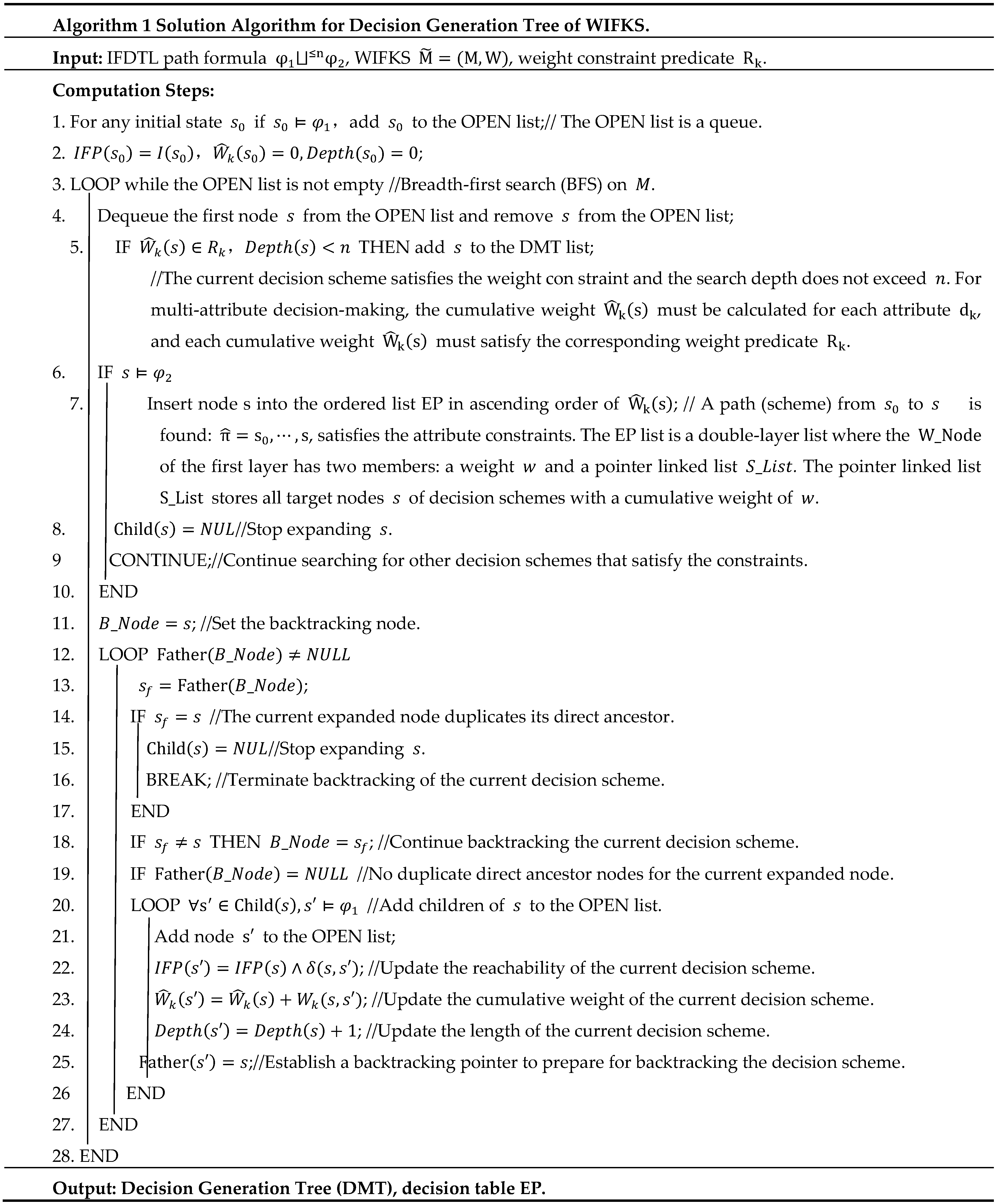
We next prove the correctness of Algorithm 1.
Theorem 2 Given an IFDTL path formula , a WIFKS, and a weight constraint predicate. Let DMT be the decision generation tree generated by Algorithm 1. Then the following hold,
(1) For any and any , if and , then is a path in DMT;
(2) If is a path in DMT, then there exist and such that and .
Proof: (1) or any and any , if . By Condition (1) of Definition 6.6, π satisfies the requirement of no repeated nodes for the sequence in Steps 8–19 of Algorithm 1. Conditions (2) and (4) of Definition 9 satisfy the constraints on the internal nodes of DMT in Step 20 of Algorithm 1. Condition (3) of Definition 9 satisfies the constraints on the leaf nodes of DMT in Step 6 of Algorithm 1. satisfies the constraints on the internal nodes of DMT in Step 5 of Algorithm 1. Thus, is a path in DMT.
(2) Let be a path in DMT; then holds. Construct an infinite path The requirement of no repeated nodes for the sequence ,…,s in Steps 8–19 of Algorithm 1 ensures that Condition (1) of Definition 9 holds. The constraints on the internal nodes of DMT in Step 18 of Algorithm 1 ensure that Conditions (2) and (4) of Definition 9 hold. The constraints on the leaf nodes of DMT in Step 6 of Algorithm 1 ensure that Condition (3) of Definition 9 holds. Therefore, .□
We next analyze the computational complexity of Algorithm 1
Theorem 3Given an IFDTL path formula, a WIFKS, and a weight constraint predicate,the time complexity of generating the decision generation tree (DMT) and decision table (EP) via
Algorithm 1
is, and the space complexity is
.
Proof: The generated DMT has at most sup(I) root nodes. For each DMT subtree, the first layer has at most branches. A node in the i-th layer has i direct ancestors and at most children, which can generate branches. Thus, the i-th layer contains at most nodes. Since the DMT has at most n layers, it contains at most leaf nodes. Each leaf node corresponds one-to-one to a path π from the root node with length no more than n, so the DMT has at most O( ) paths.
The time and space complexity of constructing the DMT are linearly related to the number of nodes in the DMT, where the DMT has at most nodes. The time and space complexity of computing the decision table EP are linearly related to the number of leaf nodes in the DMT.
Therefore, the time complexity of Algorithm 1 is . Since the space of DMT subtrees can be reused, the space complexity is .□
Corollary 1 Given an IFDTL path formula or with , a WIFKS , and a weight constraint predicate , replacing the decision scheme length n with in Algorithm 1 enables the solution for the decision generation tree (DMT) and decision table (EP) for or with . The time complexity is and the space complexity is .
By Theorem 1, for , we have . Thus, replacing the decision scheme length n with in Algorithm 1 yields the DMT and EP for or ( ). In this case, the DMT has at most leaf nodes and at most nodes in total.
We now turn to solving the IFDTL model checking problem, which is equivalent to addressing the solution of engineering decision-making problems.
5.2. Single-Attribute Engineering Decision-Making Problems Based on IFDTL Model Checking
We next present the solution algorithm for single-attribute engineering decision-making problems. A single-attribute engineering decision-making problem corresponds to the model checking of the operators ,. Algorithm 2 provides the solution algorithm for single-attribute engineering decision-making problems.
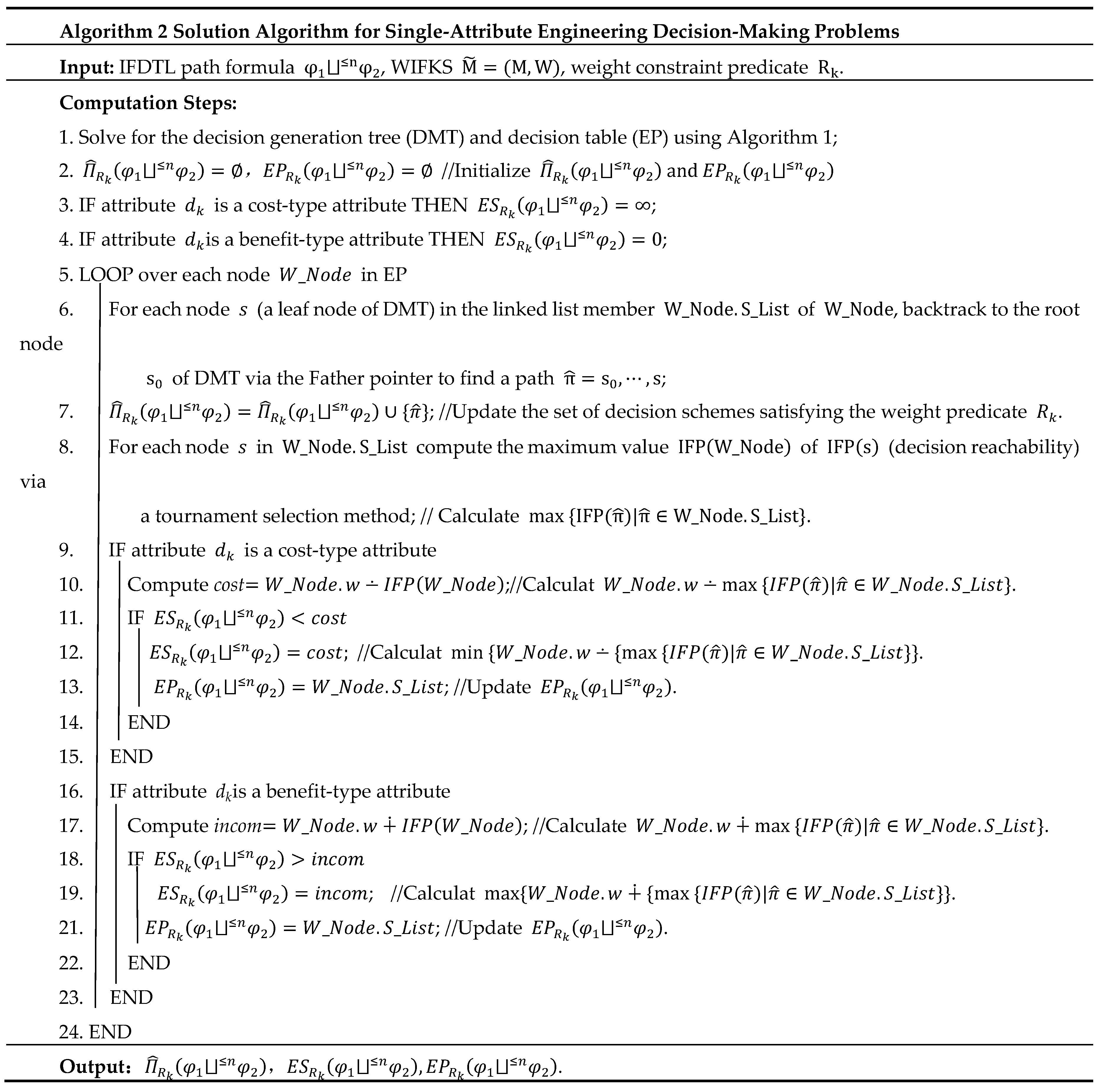
Theorem 4 Given an IFDTL path formula , a WIFKS , and a weight constraint predicate , Algorithm 2 correctly computes , and .
Proof: We first solve for the decision generation tree (DMT) and decision table (EP) using Algorithm 1. As proven in Theorem 2, the paths in DMT are in one-to-one correspondence with the kernels in that satisfy the temporal property and the weight predicate . Steps 5–7 of Algorithm 2 add all paths in DMT to the set . By Definition 10, ;
Thus, Algorithm 2 correctly computes .
Step 8 of Algorithm 2 computes the maximum value of the intuitionistic fuzzy measures for decision schemes with cumulative weight via a tournament selection method. Steps 9–15 calculate by finding the minimum value of (via tournament selection) when is a cost-type attribute. Steps 16–23 calculate finding the maximum value of (via tournament selection) when is a benefit-type attribute. By Definition 10, . Thus, Algorithm 2 correctly computes .
Steps 13 and 21 of Algorithm 2 synchronously update the set of paths with the objective function valueduring the tournament selection for . By Definition 10, ; Thus, Algorithm 2 correctly computes .□
We next analyze the computational complexity of Algorithm 2.
Theorem 5 Given an IFDTL path formula , a WIFKS , and a weight constraint predicate , let . The time complexity of computing , via Algorithm 2 is , and the space complexity is .
Proof: Algorithm 2 computes , via a tournament selection method, based on the decision generation tree (DMT, corrected from DPT) and decision table (EP) solved by Algorithm 1. The time complexity of the tournament selection is , which is the size of the decision table EP. Thus, the time and space complexity of Algorithm 2 are dominated by the complexity of solving for DMT and EP (from Algorithm 1), i.e., the time complexity is and the space complexity is . □
Corollary 2 Given an IFDTL path formula , a WIFKS , and a weight constraint predicate , let . Replacing the decision scheme length n with N in Algorithm 1 enables Algorithm 2 to correctly compute . The time complexity is and the space complexity is .
The conclusion of Corollary 2 is self-evident from Theorems 3, 4, 5 and Corollaries 1.
We next investigate the decidability and decision complexity of single-attribute decision-making problems based on IFDTL model checking.
Theorem 6 Given an IFDTL path formula , a WIFKS , and a weight constraint predicate , Algorithm 2 correctly computes with a time complexity of and a space complexity of .
Here, denotes the length of formula , which characterizes the number of IFDTL temporal operators ,,, contained in . The conclusion of Theorem 6 is self-evident from Theorem 5 and Corollary 2. The reason why the space complexity does not increase as the IFDTL formula becomes more complex is that space can be reused.
5.3. Multi-Attribute Engineering Decision-Making Problems Based on IFDTL Model Checking
We next present the solution algorithm for multi-attribute engineering decision-making problems. A multi-attribute engineering decision-making problem corresponds to the model checking of the operators . It is necessary to modify the constraint on the cumulative weight of decision schemes for a single attribute in Algorithm 1 to a multi-attribute weight constraint. Then, the qualified multi-attribute weights are weighted and fused according to attribute preferences to serve as the standard weights of decision schemes. Algorithm 3 below provides the solution algorithm for multi-attribute engineering decision-making problems.
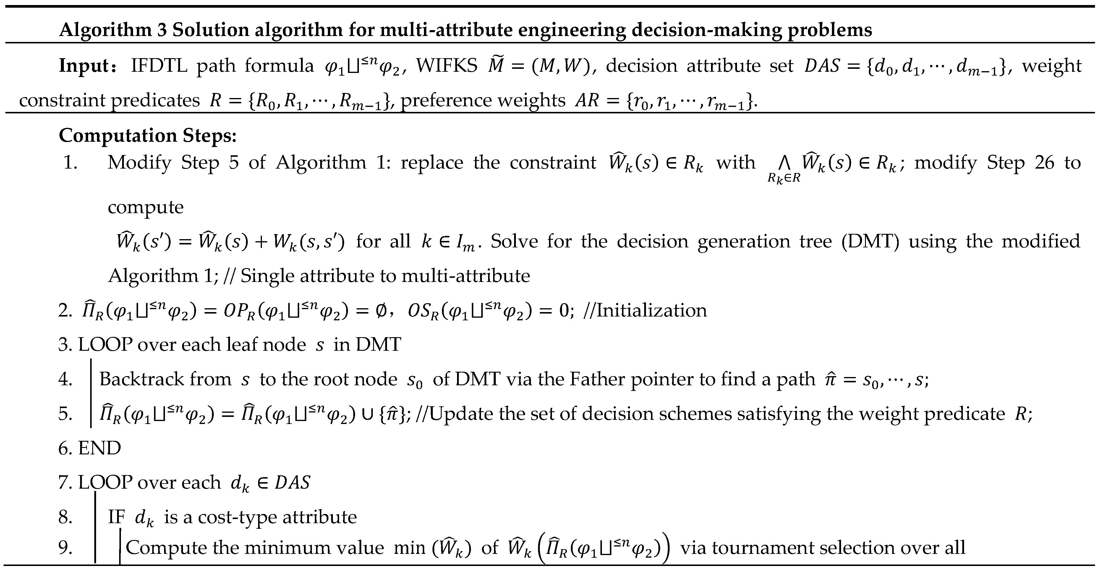
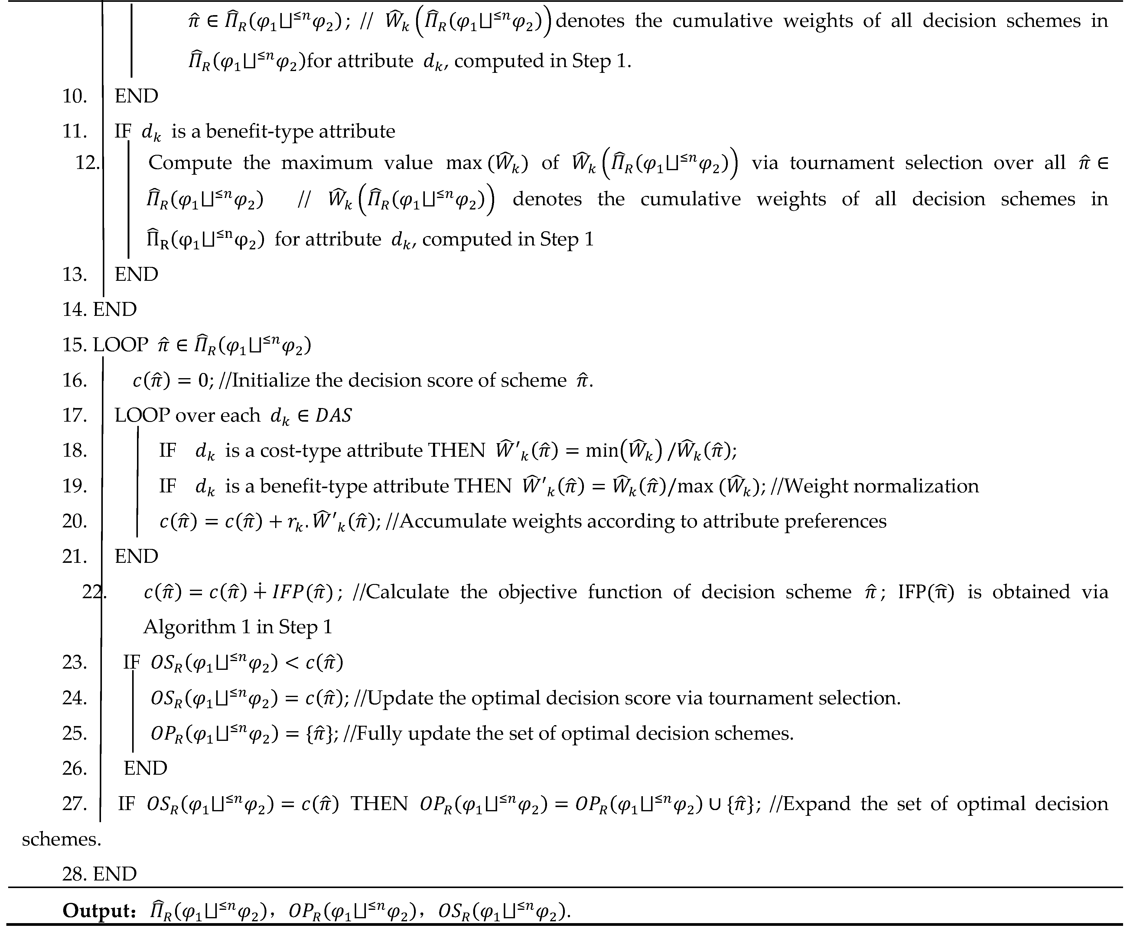
We next prove the correctness of Algorithm 3.
Theorem 6 Given an IFDTL path formula , a WIFKS , a set of weight constraint predicates , and a set of preference weights , Algorithm 3 correctly computes , , and .
Proof: Step 1 of Algorithm 3 modifies Step 5 of Algorithm 1 by replacing the constraint with , and revises Step 24 to compute for all . The modified Algorithm 1 is then used to solve for the decision generation tree (DMT) of under the constraints of and . Steps 3–5 generate a path by backtracking from each leaf node s of the DMT to the root node via the Father pointer, and add π to the multi-attribute decision scheme set . As proven in Theorem 2, the paths in the DMT are in one-to-one correspondence with the decision kernels in M that satisfy the temporal property and the weight predicate constraint . By Condition (6) of Definition 10, ;Thus, Algorithm 3 correctly computes .
For all Steps 8–10 of Algorithm 3 compute the minimum value min(Wk) of via tournament selection, and Steps 11–13 compute the maximum value of via tournament selection. Step 18 of Algorithm 3 corresponds to Equation (7) in Definition 7, and Step 19 corresponds to Equation (8) in Definition 7, which implement the normalization of the cumulative weights of decision schemes. Steps 20–22 of Algorithm 3 correspond to Equation (9) in Definition 7: they fuse the standardized weights of each attribute and the intuitionistic fuzzy measure of the decision scheme according to attribute preferences to calculate the decision score of the decision scheme π. Steps 23–27 compute the optimal decision score via tournament selection over all decision scores, and synchronously update the set of optimal decision schemes corresponding to this optimal score. Thus,
By Condition (9) of Definition 10 ; by Condition (10), . Therefore, Algorithm 3 correctly computes and .□
We next analyze the computational complexity of Algorithm 3.
Theorem 7 Given an IFDTL path formula , a WIFKS , a set of weight constraint predicates , and a set of preference weights , let . The time complexity of computing , and via Algorithm 3 is , and the space complexity is .
Proof: Algorithm 3 extends Algorithm 2 by incorporating the calculation of cumulative weights and the weight predicate constraints associated with m distinct attributes. Thus, the computational complexity is the complexity of Algorithm 2 multiplied by the size m of the attribute set. Combining this with the conclusion of Theorem 6.5, the time complexity of Algorithm 3 is . Similarly, since the space for the DMT can be reused, the space complexity of Algorithm 3 is .□
Corollary 3Given an IFDTL path formula, a WIFKS, a set of weight constraint predicates, and a set of preference weights, let.. Replacing the decision scheme length n with N in
Algorithm 1
enables
Algorithm 3
to correctly compute. The time complexity isand the space complexity is
.
The conclusion of Corollary 3 is self-evident from Theorems 6, 7 and Corollary 2. We next investigate the decidability and decision complexity of multi-attribute decision-making problems based on IFDTL model checking.
Theorem 8 Given an IFDTL path formula , a WIFKS , a set of weight constraint predicates , and a set of preference weights , Algorithm 3 correctly computes . The time complexity is , and the space complexity is .
Here, denotes the length of formula , which characterizes the number of IFDTL temporal operators contained in . The conclusion of Theorem 8 is self-evident from Theorem 7 and Corollary 3. The reason why the space complexity does not increase as the IFDTL formula becomes more complex is that space can be reused.
6. IFDTL Modeling and Verification of Health and Wellness Tourism Planning
The Shangluo section of the Qinling Mountains is located on the southern foot of the eastern Qinling Mountains. It boasts outstanding ecological and cultural resources, making it an ideal area for developing the health and wellness tourism industry. However, current health and wellness tourism planning still faces several key challenges. First, it is difficult to coordinate ecological conservation and tourism development, requiring the guarantee of wellness experience quality under strict ecological security constraints. Second, the adaptability of different wellness development models, such as ecological, cultural, and recreational ones, lacks clear definition, making it hard to provide quantitative decision support. Third, the cost, benefit, and implementation feasibility throughout the entire planning cycle are difficult to accurately predict and verify. Therefore, this paper conducts formal modeling and verification analysis on health and wellness tourism planning issues based on Weighted Intuitionistic Fuzzy Kripke Structures (WIFKS) and Intuitionistic Fuzzy Decision Temporal Logic (IFDTL).
6.1. Description of the Health and Wellness Tourism Planning Case
Health and wellness tourism planning is divided into five stages: resource investigation and demand research (planning preparation), route node selection and preliminary route design (core process 1), supporting facility planning and ecological protection design (core process 2), route optimization and trial operation debugging (final process), and acceptance and formal operation (planning completion). Each planning stage has three construction schemes: normal, priority, and emergency. The weight increments corresponding to each construction level at each stage, including investment increment, construction period increment, tourist expectation increment, and satisfaction increment, are shown in Table 2.
The intuitionistic fuzzy possibility of completion at each stage corresponding to each implementation level is shown in Table 3.
The cultural and tourism authorities require that the tourism planning scheme should achieve an expected number of tourists of no less than 55,000 and keep the total cost within 900,000 yuan. This paper aims to determine the optimal decision-making scheme under the above constraints.
6.2. Modeling of the Multi-Attribute Engineering Decision-Making Case
State is the unique initial node, representing the start of planning. For and , state denotes that the-th planning type has completed the -th stage. A virtual node is added after each stage, which does not affect the calculation results. The numbers 1, 2, 3, 4, 5 denote the respective stages; denote the implementation levels: normal, priority, and emergency, respectively; and the letter f indicates the completion of a stage task.
The WIFKS model constructed for this health and wellness tourism planning case is shown in Figure 1.
The formal description of WIFKSis given as follows:
(1) State set
(2) Intuitionistic fuzzy transition function : According to the data in Table 2, we have ;
.This setting arises because is a virtual node, and the transition from to is regarded as having maximum possibility.
(3) Intuitionistic fuzzy initial distribution : , ;
(4) Set of atomic propositions ;
(5) Labeling function : , ,,; .
(6) Investment increment weight : According to the data in Table 1, we have,
;For all .
This definition is due to the fact that is a virtual node, and no extra investment cost is required for the transition from to . The values of other investment increment weights are determined in the same manner.
The construction period increment weight , tourist expectation increment weight , and satisfaction increment weight , are defined similarly.
(7) Decision attribute set . Where denote investment increment, construction period increment, tourist expectation increment, and satisfaction increment, respectively.
6.3. Single-Attribute Engineering Decision-Making Case Based on IFDTL Model Checking
The practical constraints of the case problem are given as: “The cultural and tourism authorities require that the total investment of the completed tourism planning project shall not exceed 900,000 yuan”.
(1) The formalization of “project completion” in IFDTL is:
- (2) The set of decision schemes for “completing the project within 900,000 yuan” is formalized as the IFDTL formula: .
(3) The optimal score for “completing the project within 900,000 yuan” is formalized as:
- (4) The set of optimal decision schemes for “completing the project within 900,000 yuan” is formalized as:.
Next, Algorithm 1 is employed to generate the DMT of the health and wellness tourism planning WIFKS shown in Figure 1 under the constraints and . The result is presented in Figure 2.
Due to space limitations, Figure 2 does not label the accumulated weights of decision schemes and their feasibility (Intuitionistic fuzzy measure) obtained via iterative computation on the nodes during DMT generation.The corresponding decision scheme number, accumulated weight, and intuitionistic fuzzy measure for each leaf node are listed in Table 4.The scheme numbers correspond to each decision path in Figure 1 sequentially from left to right.
Next, Algorithm 1 is used to generate the EP table of the health and wellness tourism planning WIFKS shown in Figure 1 under the constraints and . The result is shown in Table 5.
The EP table constructs an ascending linked list with the cumulative weight as the key. Each node in this list is also a linked list that stores the IDs of decision schemes with the same cumulative weight. These are reflected in the first and second columns of Table 5. The third and fourth columns of Table 5 record the membership degree and non-membership degree of the maximum intuitionistic fuzzy measure among decision schemes with identical cumulative weights, respectively.
Next, Algorithm 2 is used to solve the single-attribute engineering decision-making problem of
under the constraints and .
By backtracking the EP table, we obtain .
Using the max–min algorithm, we get .
According to Equation (6), for all , the normalized weight of is: .
The cumulative costs “81, 83, 84, 85, 86, 87, 88, 89, 90” are normalized to: 0.90, 0.92, 0.93, 0.94, 0.96, 0.97, 0.98, 0.99, 1.00.
Model checking results show that under the constraint that the total investment does not exceed 900,000 yuan:
(1) The optimal decision score is (0.891,0.100);
(2) The optimal engineering scheme is .
In other words, the “normal level” implementation strategy is selected at all stages of the tourism planning process.
6.4. Multi-Attribute Engineering Decision-Making Case Based on IFDTL Model Checking
One of the constraints for the multi-attribute decision-making problem in this case is: “The cultural and tourism authorities require that the expected number of tourists shall be no less than 55,000, while the total investment is controlled within 900,000 yuan.” This section addresses how to determine the optimal decision scheme under these combined constraints.
(1) Project completion is formalized as the IFDTL formula:.
(2) The weight constraint predicate is:.
(3) The importance ratio of project duration to expected tourist volume for engineering decision-making is set to 4:6; that is, the preference weight is .
(4) The optimal score for completing the project with expected tourist volume no less than 55,000 and total cost within 900,000 yuan is formalized as the IFDTL formula: .
(5) The set of optimal decision schemes for completing the project with expected tourist volume no less than 55,000 and total cost within 900,000 yuan is formalized as the IFDTL formula: .
Next, Algorithm 2 is used to generate the DMT of the health and wellness tourism planning WIFKS shown in Figure 1 under the constraints and . The result is illustrated in Figure 3.
The scheme number, decision Scheme, cost, expected tourists and feasibility corresponding to the leaf nodes in Figure 3 are listed in Table 6 below.
By backtracking the DMT in Figure 3 from the leaf nodes, the set of decision schemes under and is obtained as:
Using the max–min algorithm, the minimum cost is: .
The maximum expected number of tourists is: .
Normalized costs: .
With preference aggregation, the comprehensive weights are:
The multi-attribute optimal decision score is calculated as:
The multi-attribute optimal decision scheme is:
Model checking results show that under the requirements that the expected number of tourists is no less than 55 000 and the total cost is within 900 000 yuan:
(1) The optimal decision score is ;
(2) The optimal engineering scheme is .
In other words, the priority level is adopted for three stages: resource investigation & demand research (planning preparation), route optimization & trial operation debugging (final process), and acceptance & formal operation (planning completion).The normal level is adopted for the two core stages: route node screening & preliminary design (core process 1) and supporting facility planning & ecological protection design (core process 2).
Now the constraints are strengthened. The second multi-attribute decision-making problem in this case is constrained by “The cultural and tourism authorities require that the expected number of tourists shall be no less than 55,000, the total cost controlled within 900,000 yuan, the planning period no longer than 80 days, and the satisfaction rate higher than 75%.”This section addresses how to determine the optimal decision scheme under these constraints.
Completing the project in accordance with constraints is formalized as the IFDTL formula: .
The weight constraint predicate is: ;
The importance ratio of project cost, project duration, expected tourist volume and satisfaction rate for engineering decision-making is set to ; that is, the preference weight is .
The optimal score is formalized as the IFDTL formula:;
The set of optimal decision schemes is formalized as the IFDTL formula: .
Next, Algorithm 2 is used to generate the DMT of the health and wellness tourism planning WIFKS shown in Figure 1 under the constraints and . The result is shown in Figure 4.
The scheme number, cumulative weights, and intuitionistic fuzzy measure corresponding to the leaf nodes in Figure 4 are listed in Table 7 below.
By backtracking the DMT in Figure 4 from the leaf nodes, the set of decision schemes under and is obtained as:
By the max–min method:
Minimum cost: ;
Minimum duration: ;
Maximum expected tourists: ;
Maximum satisfaction: ;
Normalized cost:;
Normalized duration:;
Normalized tourist volume:;
Normalized satisfaction:.
The multi-attribute optimal decision score is calculated as follows:
The multi-attribute optimal decision scheme is:
Model checking results show that under the requirements that the expected number of tourists is no less than 55,000, the total cost is controlled within 900,000 yuan, the planning period does not exceed 80 days, and the satisfaction rate is higher than 75%:
(1) The optimal decision score is ;
(2) The optimal engineering scheme is .
In other words, the priority level is adopted for three stages: resource investigation and demand research (planning preparation), route optimization and trial operation debugging (final process), and acceptance and formal operation (planning completion). The normal level is adopted for the two core stages: route node screening and preliminary route design (core process 1) and supporting facility planning and ecological protection design (core process 2).
6.5. Analysis of Case Results
The calculation results of the case problem illustrate that the proposed solving algorithm for engineering decision-making problems based on IFDTL model checking is effective and enables automated decision-making. An analysis of the results of the wellness tourism planning case in Section 6.4 is presented below, which demonstrates the advantages of the IFDTL model checking technique.
(1) IFKS⊂WIFKS. A WIFKS is a 2-tuple , where is an IFKS, and is a set of weight functions. Obviously, if the weight set in WIFKS is ignored, WIFKS degenerates into an IFKS. That is to say, IFKS is a special case of WIFKS. In the case, incremental weights, incremental durations, incremental expected tourist numbers, and incremental satisfaction rates at different stages of various schemes are considered, which cannot be characterized by IFKS. Therefore, IFKS⊂WIFKS.
(2) IFCTL⊂IFDTL. IFDTL extends IFCTL by introducing the operators, ; which are used to compute feasible schemes, optimal decision scores, and optimal decision schemes. In contrast, IFCTL can only verify functional properties such as “the project will eventually be completed” (), and compute , then only evaluate its intuitionistic fuzzy measure. In the case study, however, IFDTL was used to model and compute ,,,,. Therefore, IFCTL⊂IFDTL.
(3) The introduction of quality constraint operators enhances the expressive power of temporal logic. In model checking of GPoTL and IFCTL, information fusion is performed only by simple conjunction “∧” or disjunction “∨” between the system property formula and the path reachability degree, which causes information loss and asynchrony, and cannot reflect the importance degrees of system properties and path reachability to the overall decision [18,19]. However, in the IFDTL model checking proposed in this paper, the system property formula is used for functional selection to obtain the path set (Algorithm 1). Then the path reachability degree is fused with attribute weights (cost, benefit) in a weighted manner (cost attribute composition “”, benefit attribute composition “”, Definition 4, Algorithm 2). The fusion result always contains three kinds of information: system properties, path reachability, and attribute weights of decision schemes, and the information is consistently associated with corresponding paths. This is embodied in the calculation of and in the case. In multi-attribute engineering decision-making based on IFDTL model checking, weighted fusion of IFP(Π) with multi-attribute weights ensures lossless, synchronous and preference-aware information fusion (Algorithm 3). This is specifically reflected in the processes of solving ,, and in the case.
(4) The introduction of decision-making behaviors enhances the expressive power of temporal logic. PoTL, GPoTL and IFTL do not consider the selection of decision-making behaviors, which makes them unable to characterize the interactive information between the system and the external environment. This paper draws on the ideas in references [8,9] and introduces the selection of decision-making behaviors into IFCTL. For example, in the case, there are three implementation levels (normal, priority, emergency) at each stage of the project. Selecting different construction levels at different stages yields different decision schemes. Such decision-making behavior selection describes the interaction between the system and the environment, and effectively enhances the expressive power of temporal logic.
(5) By using intuitionistic fuzzy measures, IFDTL can quantify incomplete information of the system. In IFDTL model checking, the path reachability degree is an intuitionistic fuzzy number . The maximum feasible scheme measured by the intuitionistic fuzzy measure on the satisfiable scheme set is also an intuitionistic fuzzy number. The weighted fusion result of and cumulative weight is an intuitionistic fuzzy number. The optimal decision scores , are all intuitionistic fuzzy numbers. These intuitionistic fuzzy numbers contain not only the uncertainty information described by membership degree and non-membership degree, but also the incomplete information described by hesitation degree. For example, the case result , show that: The possibility that scheme is the optimal decision scheme is 81.5%. The possibility that it cannot be the optimal scheme is 17.4%. Meanwhile, the hesitation degree 1−0.815−0.174=1.1% represents the uncertain possibility whether it can be regarded as the optimal scheme.
7. Conclusion and Future Work
This paper extends the intuitionistic fuzzy Kripke structure to the weighted intuitionistic fuzzy Kripke structure (WIFKS), induces intuitionistic fuzzy computation tree logic to intuitionistic fuzzy decision tree logic (IFDTL), and studies single-attribute and multi-attribute engineering decision-making problems under the intuitionistic fuzzy framework. The main research contents are as follows:
(1) Reasonable quality constraint operators are defined to solve the problems of information loss and incomplete information quantification. The intuitionistic fuzzy Kripke structure is induced to the weighted intuitionistic fuzzy Kripke structure (Definition 1). The weights of the WIFKS naturally characterize the costs and benefits in engineering problems, and the intuitionistic fuzzy measure quantifies the uncertainty of engineering progress. Definition 2 presents information fusion operators for the cumulative weights of cost-type attributes and benefit-type attributes of decision schemes, as well as their decision feasibility, respectively. The rationality of the operators is proved (Propositions 1, 2, 3).
(2) Single-attribute and multi-attribute engineering decision-making problems are formally described. For single-attribute engineering decision-making (Definition 3), the optimal decision scheme is the one that achieves the maximum value after fusing the cumulative cost and the corresponding maximum feasibility. For multi-attribute engineering decision-making (Definition 4), the cumulative weights of decision schemes are weighted-averaged according to attribute preferences, then fused with scheme feasibility; the scheme with the highest score is selected as the optimal one. This reflects the idea of quality constraints and differentiated attribute preferences, and ensures synchronous fusion of scheme weights, feasibility and satisfaction values.
(3) The IFDTL reasoning theory is proposed. The syntax (Definition 5) and semantics (Definition 7) of IFDTL are given, where the semantic definition takes into account the uncertain selection of behaviors. Engineering decision-making problems are characterized by IFDTL formulas. respectively characterize the single-attribute satisfiable decision scheme set, the single-attribute expected decision score and the expected decision scheme under the constraints of the weight predicate and temporal property for attribute . respectively characterize the satisfiable decision scheme set, the optimal decision score and the optimal decision scheme set for m decision attributes under the constraints of the weight predicate and temporal property .
(4) Single-attribute and multi-attribute engineering decision-making problems are solved based on IFDTL model checking. Algorithm 1 generates the decision-making tree (MDT) and decision table (EP) of the WIFKS under the constraints of the weight predicate and temporal property . The paths in the MDT correspond to the satisfiable sets of decision schemes, and the nodes of the MDT store the cumulative weights and feasibility of the decision schemes. Algorithm 2 is used to compute the expected score and the expected decision scheme for single-attribute engineering decision-making. Algorithm 3 is used to compute the optimal score and the optimal decision scheme for multi-attribute engineering decision-making. The correctness of the three algorithms is proved, and their complexity is discussed.
This section focuses on the shortcomings of the current work and the prospects for subsequent research, which are elaborated in detail as follows:
(1) The IFDTL (Intuitionistic Fuzzy Decision Tree Logic) defined in this paper only focuses on completing the project in the "fastest" way, and the considered decision schemes are finite sequences. It fails to take into account the situations of "rework" or "stagnation" in the actual project implementation process, which is specifically reflected in the absence of loop settings in the model. In the subsequent research, heuristic information related to "return rate" will be introduced. When a loop occurs in the project implementation process, the cost or benefit will continue to accumulate, but the return rate will show a downward trend. In this way, the length of the loop can be restricted by setting the lower bound of the return rate or the upper bound of the cumulative cost, so as to make engineering decisions more objective and in line with the actual project situation.
(2) The computational complexity of the IFDTL model checking algorithm proposed in this paper is related to . With the continuous expansion of the state space of engineering decision-making problems, the algorithm is prone to the problem of state explosion, which affects the efficiency of decision-making. Therefore, it is of great practical significance to further explore more efficient model checking algorithms in subsequent research to improve the scalability and operation efficiency of the algorithm, so as to better adapt to large-scale engineering decision-making scenarios.
(3) At present, the research has not yet realized the effective integration of fuzzy time constraints [17,28], path reachability information and property satisfaction values. In the follow-up research, we will focus on realizing the preferential and synchronous fusion of the three, study the fuzzy temporal logic with dual constraints of fuzzy time and quality characteristics, further improve the completeness and accuracy of information expression, and apply it to the solution of engineering decision-making problems, so as to enhance the practicality and applicability of the decision-making model.
Author Contributions
X.Y. designed the syntax and semantics of IFDTL, articulated its model checking problem, and provided relevant solution algorithms. J.H. formalized the engineering decision-making problem and proposed a single-attribute engineering decision-making solving algorithm based on IFDTL model checking. W.L. formalized the multi-attribute engineering decision-making problem and presented a solving algorithm for multi-attribute engineering decision-making based on IFDTL model checking. H.R. devoted efforts to investigating the logical properties of IFDTL. F. M. furnished illustrative examples demonstrating the decision-making practice of health and wellness tourism route planning, and conducted a meticulous review of the entire paper to guarantee compliance with requisite writing standards, ensuring mathematical rigor, academic standardization and readability throughout.
Funding
This research was funded by Shaanxi Provincial Education Department Project (Grant No: 25JR064, 24JR058), Scientific and Technological Research Fund of Shangluo University (Grant NO. 25SKY002, 25SKY004), Key Research and Development Program of Shaanxi(Grant NO.2025CY-YBXM-002), Shaanxi Fundamental Science Research Project for Mathematics and Physics (Grant No: 23JSY048).
Data Availability Statement
Data are contained within the article.
Conflicts of Interest
The authors declare no conflicts of interest.
References
- Clarke, E.M.; Emerson, E.A. Design and synthesis of synchronization skeletons using branching time temporal logic[C]//Kozen D. Logics of Programs: Logic of Programs 1981. In Lecture Notes in Computer Science; Springer: Berlin, 1982; vol 131, pp. 52–71. [Google Scholar]
- Clarke, E.M.; Emerson, E.A.; Sifakis, J. Model checking: algorithmic verification and debugging[J]. Commun. ACM 2009, 52(11), 74–84. [Google Scholar] [CrossRef]
- Bianco, A.; De Alfaro, L. Model checking of probabilistic and nondeterministic systems[C]. In Proceedings of the International Conference on Foundations of Software Technology and Theoretical Computer Science; Springer: Berlin, 1995; pp. 499–513. [Google Scholar]
- Valiev, M.; Dekhtyar, M. Complexity of verification of nondeterministic probabilistic multiagent systems[J]. Autom. Control Comput. Sci. 2011, 45(7), 390–396. [Google Scholar] [CrossRef]
- Baier, C.; Kwiatkowska, M. Model checking for a probabilistic branching time logic with fairness[J]. Distrib. Comput. 1998, 11(3), 125–155. [Google Scholar] [CrossRef]
- Kwiatkowska, M.; Norman, G.; Parker, D. PRISM: Probabilistic symbolic model checker[C]. In Proceedings of the International Conference on Modelling Techniques and Tools for Computer Performance Evaluation; Springer: Berlin, 2002; pp. 200–204. [Google Scholar]
- Pan, H.Y.; Li, Y.M.; Cao, Y.Z.; et al. Model checking fuzzy computation tree logic[J]. Fuzzy Sets Syst. 2015, 262, 60–77. [Google Scholar] [CrossRef]
- Li, Y.M.; Li, L.J. Model checking of linear-time properties based on possibility measure[J]. IEEE Trans. Fuzzy Syst. 2013, 21(5), 842–854. [Google Scholar] [CrossRef]
- Li, Y.M.; Li, Y.N.; Ma, Z.Y. Computation tree logic model checking based on possibility measures[J]. Fuzzy Sets Syst. 2015, 262, 44–59. [Google Scholar] [CrossRef]
- Li, Y.M.; Ma, Z.Y. Quantitative computation tree logic model checking based on generalized possibility measures[J]. IEEE Trans. Fuzzy Syst. 2015, 23(6), 2034–2047. [Google Scholar] [CrossRef]
- Li, Y.M. Quantitative model checking of linear-time properties based on generalized possibility measures[J]. Fuzzy Sets Syst. 2017, 320, 17–39. [Google Scholar] [CrossRef]
- Liang, C.J.; Li, Y.M. Model checking of generalized possibilistic linear temporal logic with fuzzy tenses[J]. Acta Electron. Sin. 2017, 45(12), 2971–2977. [Google Scholar]
- Fan, Y.H.; Li, Y.M. Realizability of fuzzy linear temporal logic[J]. Acta Electron. Sin. 2018, 46(2), 341–346. [Google Scholar]
- Zhao, J.; Li, Y.M. Two paradigms of generalized possibility computing tree logic[J]. J. Front. Comput. Sci. Technol. 2016, 10(10), 1475–1484. [Google Scholar]
- Li, D.; Li, Y.M. The relationship between generalized possibility computation tree logic and computation tree logic[J]. J. Front. Comput. Sci. Technol. 2017, 11(10), 1681–1688. [Google Scholar]
- Li, Y.M.; Shi, Z.K.; Li, Z.H. Approximation theory of fuzzy systems based upon genuine many-valued implications—SISO cases[J]. Fuzzy Sets Syst. 2002, 130(2), 147–157. [Google Scholar] [CrossRef]
- Li, Y.M.; Wei, J.L. Possibilistic fuzzy linear temporal logic and its model checking[J]. IEEE Trans. Fuzzy Syst. 2021, 29(7), 1899–1913. [Google Scholar] [CrossRef]
- Yu, X.F.; Li, Y.M.; Geng, S.L.; et al. Fuzzy computation tree temporal logic with quality constraints and its model checking[J]. Axioms 2024, 13(12), 832–860. [Google Scholar] [CrossRef]
- Yu, X.F.; Li, Y.M.; Geng, S.L. Fuzzy linear temporal logic with quality constraints[J]. Mathematics 2024, 12(19), 3148–3177. [Google Scholar] [CrossRef]
- Li, Y.M.; Liu, W.; Wang, J.; et al. Model checking of possibilistic linear-time properties based on generalized possibilistic decision processes[J]. IEEE Trans. Fuzzy Syst. 2023, 31(10), 3495–3506. [Google Scholar] [CrossRef]
- Liu, W.N.; Li, Y.M. Optimal strategy model checking in possibilistic decision processes[J]. IEEE Trans. Syst. Man. Cybern. Syst. 2023, 53(10), 6620–6632. [Google Scholar] [CrossRef]
- Liu, W.; Wang, J.; He, Q.; et al. Model checking computation tree logic over multi-valued decision processes and its reduction techniques[J]. Chin. J. Electron. 2024, 33(6), 1399–1411. [Google Scholar] [CrossRef]
- Atanassov, K.T. Intuitionistic fuzzy sets[J]. Fuzzy Sets Syst. 1986, 20(1), 87–96. [Google Scholar] [CrossRef]
- Zadeh, L.A. Fuzzy sets[J]. Inf. Control 1965, 8(3), 338–353. [Google Scholar] [CrossRef]
- Yu, X.F.; Li, C.; Li, Y.M. Computation tree logic of intuitionistic fuzzy measures[J]. J. Front. Comput. Sci. Technol. 2017, 11(9), 1523–1530. [Google Scholar]
- Yu, X.F.; Li, C.; Geng, S.L. Research on reasoning and application of intuitionistic fuzzy linear temporal logic[J]. Fuzzy Syst. Math. 2023, 37(5), 54–68. [Google Scholar]
- Wang, Z.X.; Huang, N.; Tang, Z.L. Fuzzy multi-attribute decision-making method based on cumulative score function and accuracy function[J]. Math. Pract. Theory 2013, 43(16), 167–174. [Google Scholar]
- Frigeri, A.; Pasquale, L.; Spoletini, P. Fuzzy time in linear temporal logic[J]. ACM Trans. Comput. Log. 2014, 15(4), 1–22. [Google Scholar] [CrossRef]
Figure 1.
Case Model–Software Engineering WIFKS Model
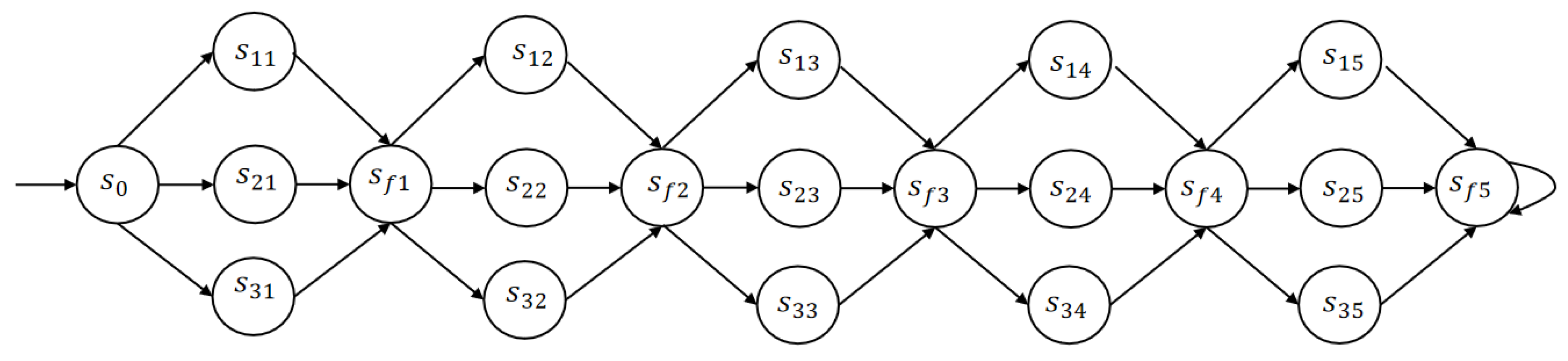
Figure 2.
DMT Generated by under the constraints and .
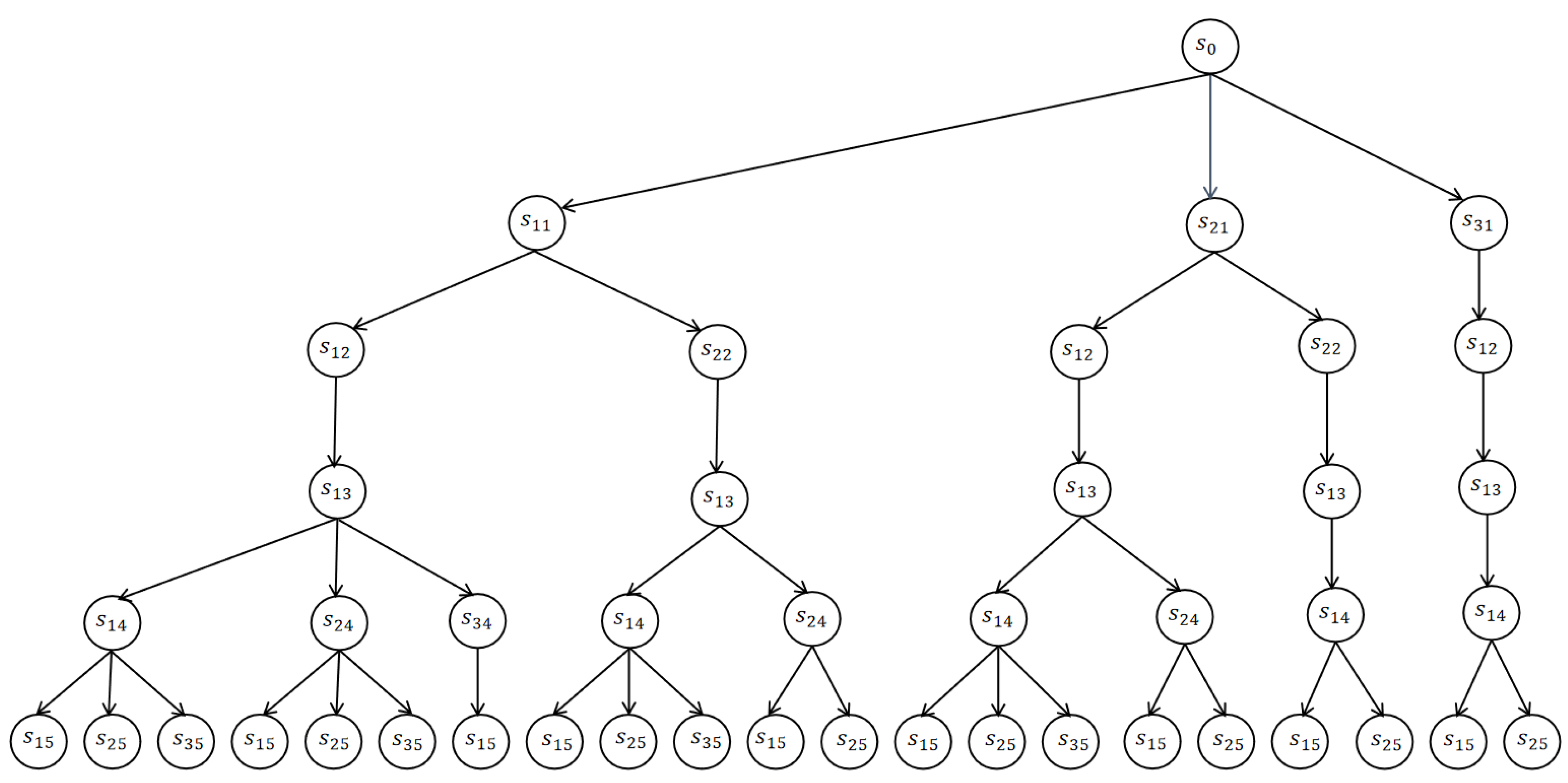
Figure 3.
DMT Generated by under the constraints and .
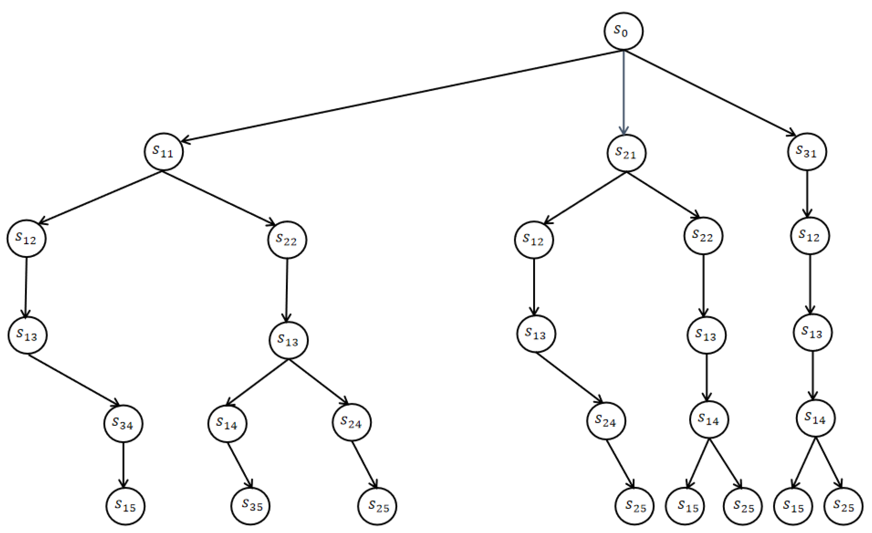
Figure 4.
DMT Generated by under the Constraints and
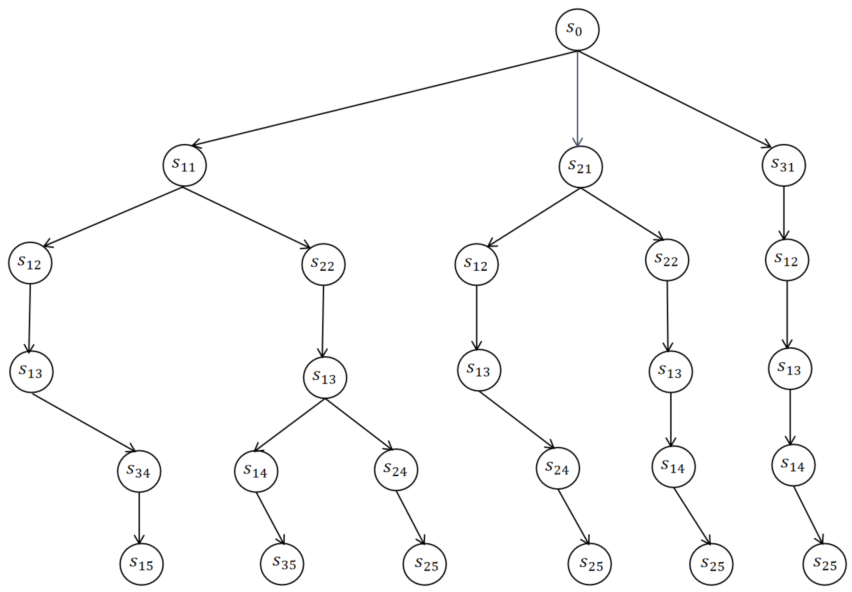

Table 1.
Comparison of Various Quantitative Temporal Logics and Their Model Checking.
| Model | KS | PKS | GPKS | GPKS | PDP | IFKS | WIFKS |
| Temporal Logics | LTL | PoLTL | GPoLTL | QFLTL | GPoLTL | IFLTL | —— |
| CTL | PoCTL | GPoCTL | QFCTL | GPoCTL | IFCTL | IFDTL | |
| Measure | Boolean algebra | Possibility measure | Generalized possibility measure | Generalized possibility measure | Generalized possibility measure | Intuitionistic fuzzy measure | Intuitionistic fuzzy measure |
| Application of Model Checking | Functional modeling and verification of classical Boolean systems. | Modeling and verification of function and performance in general uncertain systems. | Modeling and verification of function and performance in general uncertain systems. | Modeling and verification of complex uncertain systems with quality constraints. | Possibility decision-making for open systems interacting with the environment. | Modeling and verification of uncertain systems with incomplete information. | Modeling and verification of systems with incomplete information and quality constraints. |
Table 2.
Weight Increments at Each Stage for Different Schemes. (Investment Increment in 10,000 Yuan, Construction Period Increment in Days, Tourist Expectation Increment in 10,000 Person-Times, Satisfaction Increment in x%).
Table 2.
Weight Increments at Each Stage for Different Schemes. (Investment Increment in 10,000 Yuan, Construction Period Increment in Days, Tourist Expectation Increment in 10,000 Person-Times, Satisfaction Increment in x%).
| Implementation Level | Planning Preparation | Core Process 1 | Core Process 2 | Final Process | Planning Completion |
|---|---|---|---|---|---|
| Normal | |||||
| Priority | |||||
| Emergency |
Table 3.
Intuitionistic Fuzzy Possibility of Each Stage for Different Schemes.
| Implementation Level | Planning Preparation | Core Process 1 | Core Process 2 | Final Process | Planning Completion |
|---|---|---|---|---|---|
| Normal | |||||
| Priority | |||||
| Emergency |
Table 4.
Information on Leaf Nodes in the DMT.
| Scheme ID | Decision Scheme | Cumulative Cost | Feasibility |
|---|---|---|---|
| 0 | 81 | (0.88,0.11) | |
| 1 | 83 | (0.88,0.11) | |
| 2 | 85 | (0.82,0.17) | |
| 3 | 84 | (0.83,0.16) | |
| 4 | 86 | (0.83,0.16) | |
| 5 | 88 | (0.82,0.17) | |
| 6 | 89 | (0.76,0.23) | |
| 7 | 85 | (0.82,0.17) | |
| 8 | 87 | (0.82,0.17) | |
| 9 | 89 | (0.82,0.17) | |
| 10 | 88 | (0.82,0.17) | |
| 11 | 90 | (0.82,0.17) | |
| 12 | 84 | (0.85,0.14) | |
| 13 | 86 | (0.85,0.14) | |
| 14 | 88 | (0.82,0.17) | |
| 15 | 87 | (0.83,0.16) | |
| 16 | 89 | (0.83,0.16) | |
| 17 | 88 | (0.82,0.17) | |
| 18 | 90 | (0.82,0.17) | |
| 19 | 88 | (0.78,0.21) | |
| 20 | 90 | (0.78,0.21) |
Table 5.
EP Table Generated by under the constraints and .
| Total Investment Amount | Scheme ID | Membership Degree | Non-Membership Degree |
|---|---|---|---|
| 81 | 0.88 | 0.11 | |
| 83 | 1 | 0.88 | 0.11 |
| 84 | 3 | 0.85 | 0.14 |
| 12 | |||
| 85 | 2 | 0.82 | 0.17 |
| 7 | |||
| 86 | 4 | 0.85 | 0.14 |
| 13 | |||
| 87 | 8 | 0.83 | 0.16 |
| 15 | |||
| 88 | 5 | 0.82 | 0.17 |
| 10 | |||
| 14 | |||
| 17 | |||
| 19 | |||
| 89 | 6 | 0.83 | 0.16 |
| 9 | |||
| 16 | |||
| 90 | 11 | 0.82 | 0.17 |
| 18 | |||
| 20 |
Table 6.
Information on Leaf Nodes in the DMT.
| Scheme ID | Decision Scheme | Feasibility | ||
|---|---|---|---|---|
| 6 | 89 | 6 | (0.76,0.23) | |
| 9 | 89 | 6.1 | (0.82,0.17) | |
| 11 | 90 | 5.6 | (0.82,0.17) | |
| 16 | 89 | 6.2 | (0.83,0.16) | |
| 17 | 88 | 5.5 | (0.82,0.17) | |
| 18 | 90 | 5.7 | (0.82,0.17) | |
| 19 | 88 | 5.6 | (0.78,0.21) | |
| 20 | 90 | 5.8 | (0.78,0.21) |
Table 7.
Information on Leaf Nodes in the DMT.
| ID | Decision Scheme | Feasibility | ||||
|---|---|---|---|---|---|---|
| 6 | 89 | 79 | 6 | 77 | (0.76,0.23) | |
| 9 | 89 | 79 | 6.1 | 76 | (0.82,0.17) | |
| 11 | 90 | 71 | 5.6 | 80 | (0.82,0.17) | |
| 16 | 89 | 79 | 6.2 | 75 | (0.83,0.16) | |
| 18 | 90 | 71 | 5.7 | 79 | (0.82,0.17) | |
| 20 | 90 | 71 | 5.8 | 78 | (0.78,0.21) |
Disclaimer/Publisher’s Note: The statements, opinions and data contained in all publications are solely those of the individual author(s) and contributor(s) and not of MDPI and/or the editor(s). MDPI and/or the editor(s) disclaim responsibility for any injury to people or property resulting from any ideas, methods, instructions or products referred to in the content. |
© 2026 by the authors. Licensee MDPI, Basel, Switzerland. This article is an open access article distributed under the terms and conditions of the Creative Commons Attribution (CC BY) license (http://creativecommons.org/licenses/by/4.0/).
Copyright: This open access article is published under a Creative Commons CC BY 4.0 license, which permit the free download, distribution, and reuse, provided that the author and preprint are cited in any reuse.


