

Submitted:
17 August 2026
Posted:
18 August 2026
You are already at the latest version
Abstract
We describe a harmonic analysis system for predicting annual peak snow water equivalent (SWE) at SNOTEL monitoring stations operated by the Natural Resources Conservation Service (NRCS) across the western United States. The algorithm, frqsrchX, performs greedy harmonic regression on daily SWE records, identifying persistent periodic climate signals and superimposing volcanic impulse functions to account for episodic radiative forcing from major eruptions. A five-phase characterization pipeline applies distinct band-limited search strategies per site, and a two-winner selection system identifies optimal configurations by both maximum pass rate and a reliability score that balances accuracy with period stability. Validation uses out-of-sample holdout testing over fifteen graded years drawn from holdout cutoffs 2008–2025, graded by an asymmetric scale that penalizes over-prediction more harshly than under-prediction. This version reports the network re-graded under a corrected annual-peak extraction routine. The original routine assigned peaks by calendar year rather than water year, mis-crediting early-season November and December maxima by a full year. Correcting this leaves interior continental results essentially unchanged and reduces maritime results substantially, separating the network into three tiers — interior states within a third of a percentage point (pp) of zero change, maritime-influenced Idaho at −1.29 pp, and the three Pacific states clustered between −4.10 pp and −4.97 pp — a spatial structure that tracks maritime influence and independently confirms the diagnosis. Corrected average pass rates range from 87.3% (Montana, 89 sites) to 44.3% (California, 119 sites, including 86 SNOW SENSOR stations). The three commercially targeted states — Montana (89 sites), Colorado (108 sites), and Wyoming (86 sites) — achieve average pass rates of 87.3%, 86.3%, and 84.1%, with 83–91% of sites meeting the ≥80% operational pass-rate threshold under identical universal parameter search procedures and no state-specific tuning. Idaho (82 sites) remains strong at 81.8%; Washington (69 sites) falls to 76.0% under the correction and is reclassified. Utah (86 sites, 75.2%) and Oregon (78 sites, 65.7%) show mixed and poor performance respectively, and California is non-viable at 44.3%, with no station reaching the operational threshold. Among sites clearing that threshold, 53–93% achieve stable signal detection. Two hundred and six stations qualify for the two- year-ahead product. The 2026 season, the first fully prospective test, produced a near-universal over-prediction across all commercially targeted states. A station-level decomposition for Colorado, recomputed here against consistently constructed full-record baselines, attributes this outcome predominantly to rain-versus- snow partitioning during a warm snow drought — 51% of the total SWE shortfall and 57% of the model's own prediction error — rather than to a precipitation-forecasting failure. We accordingly treat warm-drought years as outside the method's scope and ungraded, while precipitation-driven (dry) snow drought, a deficit the method does forecast, is graded normally.
Keywords:
snowpack forecasting
; SNOTEL
; SNOW SENSOR
; harmonic analysis
; ENSO
; snow water equivalent
; volcanic forcing
; holdout validation
Note on This Version
Version 3 makes two corrections to Version 2 and leaves the method itself unchanged.
The peak-assignment correction. The routine that extracts annual peaks assigned each peak to the calendar year in which it occurred rather than to the water year to which it belongs. At stations where early-season accumulation in November or December is never surpassed later in the same accumulation season, this credited a real peak to the wrong year and graded it against the wrong prediction. The entire eight-state network has been re-graded with the corrected routine, using the identical input records, configuration search, and grading scale as Version 2. The correction removes optimism, and it does so in a spatially organized way: its magnitude and its incidence are both ordered by maritime character, from a hundredth of a percentage point in Colorado to more than four points on the Pacific slope. Because the reassignment rule contains no geographic term, that ordering is a prediction of the mechanism rather than an artifact of it, and we report it as a result (Section 3).
Two consequences matter for readers of Version 2. Washington's average pass rate falls from 81.5% to 76.0% and no longer belongs in the group of states above the 80% operational threshold. Oregon's stable-signal sites fall from 75.5% to 68.5%, which sharpens rather than weakens the mechanism Version 2 proposed for that state. The three commercially targeted interior states — Montana, Colorado, Wyoming — are confirmed essentially unchanged at 87.2%, 86.3% and 84.1%.
The baseline correction to the 2026 decomposition. Version 2's Table 5 mixed baseline constructions: an 18-year (2008–2025) split-half trend baseline for SWE against a full-record split-half trend baseline for precipitation. Referencing the two response variables to incomparably constructed climatologies inflated the apparent baseline model deficit and distorted the three-way split. With both baselines computed on the full record, the model's 2026 Colorado forecast stands at 96.1% of trend rather than 92.0%, observed peak SWE at 56.2% rather than 55.0%, and the decomposition shares move from 18 / 29 / 53 to 9 / 40 / 51 (Section 5.8). The qualitative conclusion is unchanged and in one respect strengthened: rain-versus-snow partitioning remains the single largest term, and it accounts for 57% of the model's own prediction error for year 2026.
Two further corrections. Version 2 declared a minimum record length of fifteen years but the pipeline did not enforce it; enforcing it removes 61 stations network-wide, including sites reaching Tier I on under two years of data. And a defect in the holdout-truncation step, unrelated to the grader, suppressed fits at 32 SNOW SENSOR California stations; correcting it raises California's average from 42.3% to 44.3% and is the reason the correction magnitude reported here is not monotonic across all eight states (Appendix D.5).
Version 3 also states explicitly four elements of the validation protocol that Version 2 left implicit — the one-year offset between holdout cutoff and graded year, the two distinct record-length gates, the treatment of snowless water years, and the water-year peak assignment itself — and corrects two errors in Version 2's supporting tables that are unrelated to either correction above (Section 4.6 and Section 4.7).
1. Introduction
Annual peak snowpack, measured as snow water equivalent (SWE), is the dominant driver of warm-season streamflow in the mountainous western United States. Water district managers, reservoir operators, and agricultural planners rely on spring snowpack predictions to make allocation decisions months in advance. Current operational forecasts from the NRCS and the National Weather Service use linear regression of current SWE conditions against historical streamflow relationships, with skill concentrated in the period from February through April when snowpack has partially accumulated. One-year-ahead forecasts — predicting the following year's peak SWE before any snow has fallen — remain an unmet need in operational hydrology.
Harmonic analysis has a long history in geophysical time-series analysis, applied to tides, solar irradiance, and paleoclimate records. The El Niño–Southern Oscillation (ENSO), Pacific Decadal Oscillation (PDO), Atlantic Multidecadal Oscillation (AMO), and solar activity cycles all modulate western U.S. precipitation and snowpack on interannual to decadal timescales [5–9]. Appendix A reports the period structure of each of these indices, obtained by single-period harmonic search, and documents how that structure was used to define the narrow search bands employed in Section 2.7. If these signals are sufficiently periodic and persistent, they should be identifiable in the station-level SWE record and extrapolatable one year forward. The central hypothesis of this work is that greedy harmonic regression, properly constrained against overfitting and augmented with volcanic impulse functions, can extract this predictive signal at individual SNOTEL station scale.
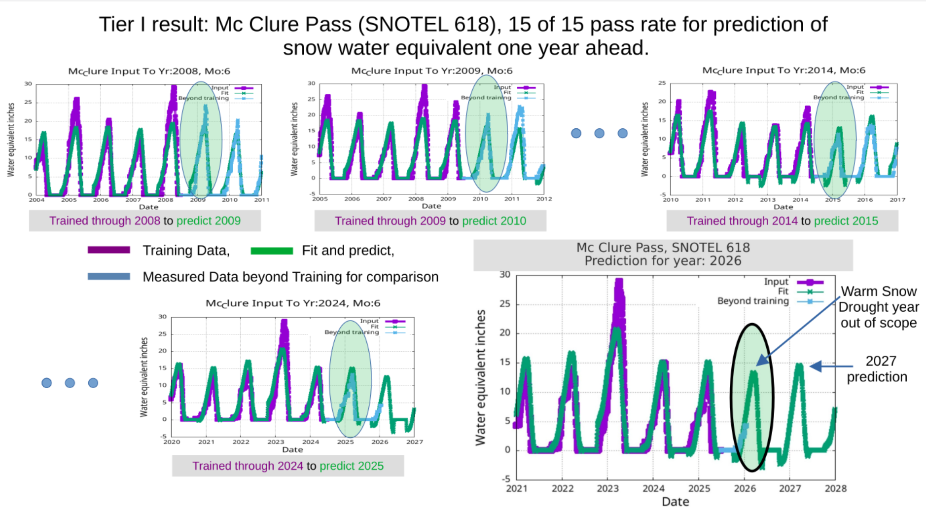
This paper describes the frqsrchX algorithm and its supporting pipeline, reports validation results across the eight-state network, and characterizes the regional spectral structure that drives performance differences across states (see Figure 1 for one example and Appendix B for a partial report on another site). Companion papers establish the physical basis for the methodology: Higginbotham (2026a) [1] examines the role of water vapor and volcanic eruptions in atmospheric radiative forcing, and Higginbotham (2026b) [2] validates harmonic analysis over a 350,000-year Antarctic ice core record.
Section 2 describes the method, with four elements of the validation protocol now stated explicitly that Version 2 left implicit. Section 3 is new: it documents the peak-assignment error, its mechanism, the station-level and network-level evidence establishing the diagnosis, and the spatial gradient the correction produces. Section 4 reports corrected results for the full network. Section 5 revises the discussion, including a recomputed 2026 decomposition. We report both corrections in full rather than presenting the corrected method as though it had always been in use: forecasts issued for the 2026 season were generated and graded under the original routine, and users holding those forecasts need to know which grader produced the reliability figures attached to them.
2. Data and Methods
2.1. Station Network and Input Data
The NRCS operates the SNOTEL (SNOwpack TELemetry) network of automated monitoring stations across the western United States, with 880 stations in 13 states [3]. A related network of SNOW SENSOR stations uses different detection equipment — pressure sensing rather than acoustic pillows — but records the same SWE measurement and is included in the NRCS database on the same reporting interface. For California in particular, a substantial fraction of the analyzed sites are SNOW SENSOR stations (86 of 118 analyzed); results for these sites are included in the California totals and are treated as directly comparable to SNOTEL results for the purposes of harmonic prediction. Stations measure SWE, precipitation, air temperature, and other meteorological variables at typical elevations of 6,000–11,000 feet. Records for the longest-running stations extend from the late 1970s to present, providing 38–47 years of annual observations. Stations with fewer than 15 years of record are excluded. This rule is enforced against the record span recorded at the time of milli-year conversion (early in the computation), before any holdout truncation, so it is available even for stations that produce no fit; 55 stations across the eight states fall below it and are excluded from all results reported here. Record end dates are taken from the same source. In the seven interior and Cascade states every station reports to the end of the analysis period, but 18 California SNOW SENSOR stations have discontinued or intermittent records ending between 2021 and 2025, most of them with 30 or more years of prior record. Graded-year counts therefore vary by station in California, and its pass rates are computed over each station's available years.
We use daily reported SWE values from the NRCS data site as input to the analysis. The model is fit to the daily series; annual peaks are then extracted from both the observed and the fitted daily series and compared for grading. While the basic algorithm is a least-squares fit, fit quality is not the attribute used to grade configuration performance. Instead, the fit configuration is graded on its ability to predict the peak SWE of the water year following the truncated input, as developed in Section 2.3 and Section 2.8.
We report results for eight states: Colorado (CO), Montana (MT), Wyoming (WY), Idaho (ID), Washington (WA), Utah (UT), Oregon (OR), and California (CA). Station rosters in this version differ from Version 2 for three reasons, all documented in Appendix D: six stations initially absent from the Version 3 summaries because of an output defect unrelated to the analysis, since recovered; enforcement of the ≥15-year record rule stated above, which Version 2 declared but did not apply; and a defect in the input-preparation stage that suppressed fits at 32 California SNOW SENSOR stations, since corrected.
2.2. The frqsrchX Algorithm
The frqsrchX algorithm (implemented in Fortran) performs greedy harmonic regression. The model combines two categories of basis functions: (1) volcanic impulse functions, fixed and provided as input parameters, and (2) harmonic functions of the form A·sin(2πt/P + φ), where P is the period searched and A and φ are computed analytically via least squares once P is determined. The algorithm builds the model incrementally: at each step it searches candidate periods, selects the one most reducing residual variance, tests it against a constraint system, and either accepts or rejects it. Accepted periods are associated with period "slots" to allow comparison of periods across holdout years independent of the order in which they were accepted.
Data preprocessing applies several steps: (1) time conversion to milliYears (mY), where 1,000 mY = 1 year; (2) removal of the mean annual cycle via split-half averaging (Figure 2); and (3) residual smoothing to reduce high-frequency noise (Figure 3). Split-half averaging computes the mean annual cycle separately over the early and late halves of the station record and interpolates linearly between two anchors placed at the midpoints of those halves; the construction is therefore trend-aware. The fit is performed on the residual and the average is added back. No explicit temporal weighting is applied within the harmonic basis; the algorithm treats all years in the training window with equal weight.
The linear baseline is computed once and held fixed across holdouts. The split-half average is estimated from the complete station record before any holdout truncation, and the same linear baseline is used for every holdout. This is deliberate. A baseline re-estimated per holdout would score each graded year against a different climatology, and the earliest holdouts — which have the least data behind them — would rest on the noisiest estimates, adding variance to the reference precisely where it is least well determined. Holding it fixed means the only quantity varying across holdouts is the harmonic fit, which is what the validation is testing. This linearly interpolated baseline represents long variation that includes periodic variation longer than the input time interval. The averaging is assumed to be sufficiently stable to extrapolate linearly beyond the midpoint year of the years that were averaged.
The consequence is that a given holdout's baseline incorporates years later than its own cutoff. The magnitude of that dependence is small and directly measurable. Across the eight-state network the mean annual cycle changes between the early and late halves of the record by 7.3% to 13.7% in amplitude (Table 11), a slowly varying quantity carrying essentially no information about the interannual variation the model is asked to predict. Because the model is graded on absolute peak SWE rather than on anomalies, the baseline enters the comparison directly rather than cancelling; we therefore state the dependence rather than treat it as negligible by construction.
The seasonal mask. Each station carries a trapezoid window over its accumulation season, defined by five dates: the start and top of the autumn ramp, the start and end of the melt-out ramp, and a window close exactly one year after the ramp-up start. Typical values are a ramp of about a week at each end and a plateau of roughly 210 days. The window is applied to the fit basis functions, not only to the input data, so it forms part of the model rather than a preprocessing step.
The mask is derived from the second half of the record and, like the linear baseline, is fixed across holdouts. The reasoning is the same and is specific to a forward-looking method: the fit is extrapolated one year beyond the training window, so the season window that matters is the one prevailing near the end of the record, not an average over a regime that no longer holds. Season timing is itself regionally coherent — median season opening ranges from late September in Montana and Wyoming to late October in Oregon, and median melt-out from May 29 in Utah to June 18 in California — which indicates the mask is capturing real phenology (climate influence) rather than fitting noise.
A mask that varied within a record was considered and rejected. Because the mask multiplies the basis functions, a drifting window makes the basis non-stationary, and the period-stability metric of Section 2.9 exists to measure whether the same periods are recovered across independent holdout windows; a time-varying basis could induce apparent period drift that the metric would misread as instability. The perturbation such a drift would introduce is also quantifiable: a melt-out knot drifting linearly across a 40-year record perturbs the basis functions by roughly 10⁻³ in normalized correlation at three days of drift, rising to 2.8 × 10⁻² at thirty days, uniformly across the period band. The tightest orthogonality threshold in use is 0.02 (Section 2.4), so drifts of a few days are immaterial while a month-scale drift would not be. Peak SWE is in any case insensitive to the window edges: observed peaks fall near fractional year 0.22–0.27 against a melt-out ramp beginning near 0.44, sixty days or more inside the plateau.
2.3. Annual Peak Extraction and Water-Year Assignment
Because the graded quantity is an annual peak, the assignment of each peak to a year is part of the method rather than an implementation detail. This subsection states the rule; Section 3 documents the error it corrects.
A snowpack accumulation season spans the turn of the calendar year. Snow falling in November and December of calendar year Y is early-season accumulation for the pack that typically reaches its maximum in the spring of Y+1 and melts out that summer; it belongs to water year Y+1. At most stations the spring maximum exceeds any December value and the distinction is invisible. At stations where a large early-accumulation event produces a December maximum that is never surpassed — a condition intermittant on Cascade and coastal stations and rare in the interior — the distinction determines which year the peak is credited to.
The peak extractor therefore operates as follows. The daily series, observed or fitted, is scanned for maxima. A maximum occurring at fractional year greater than 0.833 (past early November) is rolled forward: the year index is incremented and the fractional part reduced by 1.0, so a December-Y maximum is recorded as water year Y+1 with a negative fractional part. Each water year is then searched across its full November-through-May window and yields exactly one peak. The peak record carries a signed fractional part (year, signed fraction, value). The rule is applied identically to the observed and fitted series, so the grading comparison is between the observed water-year peak and the model's predicted water-year peak.
2.4. Overfitting Constraint: FNCA
The FNCA (Fractional Normalized Covariance Allowed) constraint prevents overfitting by rejecting candidate periods whose basis functions are insufficiently orthogonal to those already accepted. When a candidate period passes the minimum period separation pre-filter, the algorithm computes two normalized covariance matrices — one measuring geometric overlap between basis functions (Normalized Basis Covariance), one measuring amplitude stability (Normalized Parameter Covariance). If any off-diagonal element involving the candidate exceeds the FNCA threshold in either matrix, the candidate is rejected. FNCA values tested range from 0.02 (very tight, requiring near-orthogonality) to 0.40 (loose, permitting moderate correlation).
2.5. Band-Limited Search: MASK
The MASK parameter restricts the period search to specified frequency bands for the first MASK_INT period slots. Without MASK constraints, the algorithm can identify spurious high-R² periods lacking physical grounding. Two specification formats are supported: boundary pairs defining low–high band edges, and center/half-width notation for precision bands.
The bands are of two distinct origins. Those used in Phases B and D are broad and are taken from published periodicities for the ENSO, decadal and solar-cycle ranges. The 35 narrow precision bands of Phase C are derived directly from the period spectra of five climate indices (SOI, PDO, AMO, PNA, TSI); Appendix A reproduces those spectra and documents the correspondence band by band.
A further constraint operates within the band system. At most one period may be accepted from any band: when a period is selected, the band containing it is removed from the search, and later slots must draw from the bands that remain. This is categorical rather than numerical and acts independently of the FNCA orthogonality test of Section 2.4, which compares a candidate against the periods already accepted rather than against the region of the spectrum it occupies.
The interaction between this rule and MASK_INT determines how strongly each phase is constrained. In Phases B and D, MASK_INT is set equal to the number of bands — three and two respectively — so every band is guaranteed to contribute exactly one period before the remaining slots are searched without constraint. Phase D therefore always carries one ENSO-band period and one long-period-band period, even where an unconstrained search would have preferred two periods from the same region. In Phases C and E the band count exceeds the maximum of four periods, so every accepted period is drawn from a distinct band. The band and orthogonality constraints act independently and neither substitutes for the other: controlling for the number of periods, the FNCA threshold of the winning configuration is statistically indistinguishable across the five phases, so the band system does not relieve the covariance test of work it would otherwise do.
2.6. Volcanic Forcing Framework
Volcanic eruptions inject aerosols into the stratosphere, reducing solar transmission and causing short-term cooling that manifests in snowpack records as anomalous years unrelated to the periodic climate signal. Without volcanic impulse functions, the algorithm attempts to fit these step changes with sinusoids, corrupting period selection. Four transfer functions are used in production: (V1) Hunga Tonga stratospheric water vapor injection (peak 2023.0, exponential decay); (V2) 2018 warm snow drought impulse (center 2017.5); (V3) Pinatubo fast component (center 1991.8); and (V4) Pinatubo slow component (center 1991.4). The physical basis is established in Higginbotham (2026a) [1]. An independent validation — applying 23 eruption impulses and 15 periodic functions to 60 years of atmospheric transmission data — achieves R² = 0.94 (Figure 4), demonstrating that the parameterization captures real stratospheric aerosol physics with high fidelity (Walker Water LLC, internal technical report, 2026).
The role these functions play differs between the two applications, and the distinction matters for how they should be read here. Against atmospheric transmission data they are impulse functions in the direct sense: transmission responds to stratospheric aerosol loading almost immediately, so the fitted function tracks the eruption itself. Against snowpack they act as transfer functions. Snowpack responds to an eruption only through an intervening chain — radiative forcing, temperature, storm track, precipitation phase — each stage of which introduces its own delay and shape. The fitted function therefore represents the aggregate response of that chain to a forcing whose timing is known independently, not the forcing itself. This is why the centres and decay constants used for snowpack are not simply the eruption dates, and why their decay behaviour is the least well constrained part of the parameterization (Section 5.4).
2.7. Five-Phase Characterization Pipeline
Each station is characterized through five independent phases, each employing a distinct search strategy. Phase A (OPEN) applies no MASK constraints, providing an unconstrained baseline. Phase B (Mod_000) uses three broad bands covering the ENSO band (2,700–2,900 mY), a mid-range band (~6,000–7,500 mY), and an extended long-period band (10,500–17,000 mY). Phase C (Mod_00C) applies 35 narrow precision bands (1% half-width) derived from climate index spectral peaks. Phase D (Mod_00D) uses minimal two-band constraints covering only the ENSO and extended long-period bands, so that its first two periods are drawn one from each.
Phase E (Mod_00E) applies 10 broad bands spanning the sub-decadal through decadal range. Because at most one period may be taken from each band (Section 2.5), Phase E samples widely across the spectrum while preventing several accepted periods from clustering within a single spectral feature; this, rather than the presence of bands as such, is the substantive distinction from the unconstrained Phase A.
All phases test the same configuration order (Appendix C).
2.8. Validation Protocol and Grading
Holdout and prediction indexing. For a holdout year N, all data from approximately June of N forward is removed from the fit. The graded quantity is the peak SWE of water year N + 1 — the year after the holdout cutoff. The holdout year is not the year being graded. This simulates the real-world condition in which a forecast is made mid-season, before any snow has fallen in the target year. Two- and three-year-ahead predictions are produced from the same fit and reported, but do not enter the pass rate; the pass rate is the one-year-ahead figure only. The two-year-ahead horizon underpins the two-year product of Section 4.8.
Holdout set. Holdout cutoffs run 2008–2025, yielding one one-year-ahead grade each, for a nominal eighteen. Three predicted years are withheld from grading, leaving fifteen graded years.
Record-length gates. Two distinct per-station gates apply, and they produce different denominators for different metrics. The grading inclusion gate is 5 years: a holdout enters the pass-rate denominator if at least 5 years of record precede it, and is excluded below that. A holdout meeting the gate for which the algorithm produced no viable fit is counted as a failure, not an exclusion — it is a real prediction failure. The stability gate is 15 years: only holdouts with a training span of at least 15 years contribute to ValueCV and the stability classification (Section 2.9). Because the oldest year of record is fixed for all holdouts, later cutoffs have longer training spans, so the most recent holdouts are the data-rich ones that clear the 15-year gate. A short-record holdout can therefore count toward the pass rate without contributing to stability, and pass-rate N and stability N differ for the same station by design.
In addition, the maximum period allowed in the search is 90% of the total time interval of the input to the greedy algorithm.
Snowless water years. A water year with observed peak SWE of zero is graded as a failure when the model predicts non-zero accumulation. Earlier versions of the grader returned a perfect score in this case through a division guard, producing spurious A+ grades at stations with occasional snow-free years. Water years with small but non-zero observed peaks are graded normally.
Outside-scope years. A small number of years are withheld from grading because they are dominated by forcing the SWE-based periodic model is not designed to represent. The classification is retrospective and cause-based: it rests on historical knowledge of the forcing — a recorded major eruption, or a season identified after the fact as a warm snow drought — and never on whether the SWE prediction for that year succeeded, so it cannot select for prediction errors. Such years are not removed from the training fit; they remain in the fit, compensated by the localized transfer functions of Section 2.6, and are withheld only from the pass rate. Those functions absorb the snowpack response to a forcing whose timing is known from the historical record; they do not predict the forcing, which is precisely why the years concerned are withheld from grading rather than counted as successes. Two classes qualify:
- Major volcanic forcing: a VEI 5 or greater eruption in or shortly before the target water year, taken as a matter of historical record.
- Warm snow drought: a season classified as warm, or warm-and-dry, in the temperature-versus-precipitation sense, in which near-normal cool-season precipitation fails to accumulate as snowpack because of anomalous warmth — diagnosed from a positive cool-season temperature anomaly together with an SWE shortfall not matched by a precipitation shortfall. A dry snow drought, in which the snowpack shortfall reflects a genuine precipitation deficit, lies within the method's scope and is graded normally.
By these criteria 2023 qualifies under the first class and 2018 under the second; both carry compensating impulse functions and are ungraded. 2026 is also ungraded, for the distinct reason discussed in Section 5.6.
Grading scale and tiers. Grading uses an asymmetric scale (Appendix B): over-prediction is penalized more harshly than under-prediction, because shortfall destroys client trust and creates operational emergencies. Over-prediction enters the failing range at +27% deviation; under-prediction fails at −31%. A grade of C− or better constitutes a pass. Tiers are assigned by pass rate: Tier I ≥85%, Tier II ≥75%, Tier III <75%. The reliability score is (1 − VCV²) × PassRate. Grading is performed entirely by software with no human intervention.
2.9. Period Stability Metric (VCV)
Period stability (VCV) is computed from the slot-based period distribution across holdouts. Each holdout's periods are assigned to frequency slots; adjacent slots are merged if their combined coefficient of variation is below 5%; slots appearing in more than 50% of mature holdouts are considered dominant. Per dominant slot, instability is the maximum of the within-slot coefficient of variation and (1 − √occupancy). VCV is the worst instability across dominant slots. When no slot reaches the dominance threshold — scattered period selection — VCV is set to 0.7071, which is √0.5 and is chosen so that the reliability score (1 − VCV²) × PassRate retains exactly half of the pass rate. Because 0.7071 exceeds the 0.30 boundary, a station with scattered period selection is necessarily classified unstable however high its pass rate; 77 stations across the eight states fall in this category. Only holdouts with a training span of at least 15 years contribute. Stability categories: STBL (VCV < 0.10, consistent signal detection), MDRT (0.10–0.30, moderate variation), USTBL (≥0.30, scattered or unreliable periods).
Provenance caveat. Slot-based VCV is preferred wherever it is available; where it is absent a site falls back to a row-position VCV derived from the ordered-difference-plot output. The two are not interchangeable, so a site whose provenance changes can change its reported stability class without any change in its period selections. In the results reported here the slot-based value is available for every station in seven of the eight states. California is the exception: of the 122 California stations for which a stability value could be computed, 35 carry a slot-based VCV and the remainder fall back to the row-position value, so its Table 4 row alone pools two metrics and should be read with that in mind. Table 5, which restricts to sites clearing the 80% score gate, is uniformly slot-based in every state.
3. The Peak-Assignment Correction
3.1. The Defect
The annual-peak extraction routine assigned each peak to a calendar year by searching the calendar year for maximum snow water equivalent. This ignored that a snow season generally starts late in the year prior to the spring peak of a given year – a spring peak being typical for almost all interior western states (UT, CO, WY, MT). Applied to a quantity whose accumulation season crosses the turn of the calendar year, this rule mislabels early-season maxima. A peak occurring in December of calendar year Y belongs to water year Y+1 (Section 2.3), but is recorded as year Y. Extending the method toward Pacific States, where episodic weather becomes increasing more significant. triggered the defect.
The consequence is not a constant offset error. In any year where a December maximum exceeds that calendar year's spring maximum, the December value wins the year-Y slot and is graded against the model's year-Y prediction — a real observation matched to the wrong forecast. In years where the spring maximum is larger, no error happens. The error is therefore amplitude-dependent and year-irregular: it appears at some stations in some years and not others, it cannot be removed by a bias adjustment, and it leaves no recognizable signature in aggregate statistics.
The routine runs on both the observed and the fitted series, so it is not confined to scoring. It determines the peak comparison on which every holdout grade rests. Success with interior states led to a false sense of adequacy in application to the Pacific states.
A second, independent defect affected water years with an observed peak of zero. A division guard returned a perfect score in that case, so a station with an occasional snow-free year received spurious A+ grades for years in which the model predicted substantial snow.
3.2. Grader Lineage
Four versions of the grading routine exist. Naming them explicitly matters because the graded results are not identifiable from the summary files themselves (Section 5.10). While four versions are named, only grades associated with version PD1, and now PD3.1 were reported.
PD1 — the original 2025 routine. Calendar-year assignment, peak selected by amplitude within the calendar year. All Version 1 and Version 2 results were produced under PD1, as were the forecasts issued for the 2026 season.
PD2 — an intermediate diagnostic version that excluded all samples past fractional year 0.6. This incidentally excludes December (fractional year ≈ 0.92), so PD2 never mis-selects — but it is blind to December and silently drops December-dominant years from the graded set entirely. PD2 is not correct and its results are not reported here.
PD3 — implements the water-year reassignment of Section 2.3. Every water year is searched across its full accumulation window and graded exactly once. A timing heuristic present in the earlier versions, which compared a peak's fractional position against a per-station reference, was removed: once peaks are assigned to the correct year it serves no purpose, and its removal also retires a known weakness, since that reference was unreliable on short holdout records.
PD3.1 — canonical. PD3 plus the snowless-year fix: a water year with observed peak zero grades as a failure when the model predicts non-zero accumulation.
Grading arithmetic is identical across PD2 and PD3, verified on 23 shared years with matching observed and predicted values — same deviation, same percentage, same letter grade. PD3 differs from its predecessors only in peak selection, never in scoring. The comparison between graders is therefore clean: any change in a pass rate is attributable to which peaks were graded, not to how they were scored.
3.3. Station-Level Verification
Two stations with long records were examined under all four graders, with peak tables inspected year by year.

Table 1.
Pass rates and graded-year counts at two verification stations.
| Station | PD1 | PD2 | PD3 | PD3.1 (canonical) |
|---|---|---|---|---|
| 710 Railroad Overpass (OR) | 13.8% (29 yr) | 25.9% (27 yr) | 22.7% (44 yr) | 18.2% (44 yr) |
| 726 Saddle Mountain (OR) | 46.6% (35 yr) | 20.0% (31 yr) | 19.6% (46 yr) | 19.6% (46 yr) |
The denominators are the first thing to read. PD1 and PD2 graded 29 and 27 years at station 710 and 35 and 31 at station 726; PD3 grades 44 and 46 — every water year in each record, with none missing. The earlier graders were not merely disagreeing about grades; they were computing pass rates over different and incomplete populations of years.
The two stations move in opposite directions under the identical fix, which is the signature of a correction rather than a bias. Station 710 rises: under PD1, phantom December peaks graded against the wrong year's prediction were near-certain failures that padded the failure count, and removing them raises the rate. Station 726 falls: under PD1 a favorable subset of calendar years was graded, and grading every water year honestly lowers it. Station 726 had six December peaks reassigned (1986, 1995, 1997, 2009, 2013, 2015) with values up to 20.1 inches; all six fail under PD3 because the fit misses them. Station 710 had fourteen such reassignments.
The PD3 → PD3.1 step changed exactly two rows at station 710 — water years 1983 and 2003, both snow-free, moving from a spurious perfect score to failure. Every other row is identical. Station 726 has no snow-free years and was unchanged by the step, confirming that the snowless-year fix is surgical.
Full-record verification alone is not sufficient, because production runs use short holdout windows. A holdout test was therefore run at station 726 with a 2019.5 cutoff, grading water years 2020–2022. PD3.1 graded exactly those three years, consecutive, with no drops and no leakage into the training period, and made the correct boundary call on the ambiguous case: the 2022 observed peak fell at fractional year +0.016 — within days of January 1 and the largest value of its water year — and was correctly retained in water year 2022 rather than rolled back into 2021. Grades were D, C−, F, for 33.3%. This case matters because production runs grade short windows, not whole records. Over the 44 years of a full-record test a single mis-assigned boundary year shifts the pass rate by about two percentage points and is invisible; in a three-year holdout window the same year is worth 33 points. The boundary rule therefore had to be verified under the short-window conditions the production pipeline actually uses.
3.4. Network-Wide Effect: The Maritime Gradient
Each state was re-run under PD3.1 on the same input records and compared against its own original PD1 summary, restricted to stations present in both runs.
Table 2.
PD1 → PD3.1 correction by state, common stations only.
| State | Character | Common sites | PD1 mean | PD3.1 mean | Δ (pp) | Sites changed | % changed |
|---|---|---|---|---|---|---|---|
| Colorado | interior continental | 107 | 86.26% | 86.20% | −0.06 | 5 (3↓ 2↑) | 4.7% |
| Wyoming | interior continental | 86 | 84.18% | 84.05% | −0.13 | 4 (3↓ 1↑) | 4.7% |
| Montana | interior continental | 88 | 87.65% | 87.35% | −0.30 | 6 (5↓ 1↑) | 6.8% |
| Utah | interior / Great Basin | 86 | 75.54% | 75.22% | −0.32 | 8 (6↓ 2↑) | 9.3% |
| Idaho | maritime-influenced | 82 | 83.07% | 81.78% | −1.29 | 17 (16↓ 1↑) | 20.7% |
| California | maritime, AR-dominated | 118 | 48.36% | 44.26% | −4.10 | 88 (73↓ 15↑) | 74.6% |
| Washington | maritime (Cascades) | 68 | 80.12% | 75.97% | −4.15 | 48 (45↓ 3↑) | 70.6% |
| Oregon | maritime | 78 | 70.65% | 65.68% | −4.97 | 55 (50↓ 5↑) | 70.5% |
| All | 713 | −1.87 | 235 | 32.6% |
The correction separates the network into three tiers, and two independent quantities produce the same separation.
The magnitude is negligible in the four interior and Great Basin states, which cluster between −0.06 and −0.33 percentage points; an order of magnitude larger in maritime-influenced Idaho at −1.29; and an order of magnitude larger again in the three Pacific states, which cluster between −4.10 and −4.97. Within the interior group and within the maritime group the ordering carries no meaningful information — the spread inside each is smaller than the gap between them.
The incidence — the fraction of stations whose pass rate moved at all — reproduces the same three tiers from an independent measurement. The interior states cluster between 4.7% and 9.3%, Idaho doubles that at 20.7%, and the Pacific states jump to a band of 70–75% within which they are again indistinguishable. On maritime stations the correction is not an occasional event: it touches roughly seven stations in ten.
We report the tiered structure rather than a monotonic ranking because that is what the data support. An earlier version of this analysis reported a monotonic ordering across all eight states; it depended on a California figure since found to be contaminated by a separate defect in input preparation (Appendix D.5), and it does not survive correction of that defect. What survives is the three-tier separation and the factor of thirty between its ends.
The direction is uniform where it matters. Every maritime state moved down on balance, and Washington moved down at 45 of the 48 stations that changed at all. California's SNOTEL and SNOW SENSOR sub-populations behave alike, so sensor type is not a confounder. The original routine never understated skill in the states where the defect was active; the correction removes optimism, concentrated exactly where December-dominant accumulation years hide.
3.5. Why the Gradient Is a Physical Result
The error requires a specific physical condition to activate: an early-season accumulation maximum in November or December that is never surpassed later in the same water year. That condition is a property of the precipitation regime. Maritime stations on the Cascade and coastal ranges receive large, warm, moisture-laden storms early in the season and frequently reach an early maximum; interior continental stations accumulate more gradually through a colder winter and peak in spring. December-dominant years are therefore common on the west side and rare in the Rockies.
The observed spatial structure of the correction is what that mechanism predicts, and it was not used in constructing the fix. The reassignment rule contains no geographic term, no state parameter, and no station-level tuning; it is a single threshold on fractional year applied identically at all 713 stations. That a uniform rule produces a clean maritime-to-continental gradient is independent confirmation that the diagnosis is correct — the effect is keyed to the physical condition the mechanism requires.
This gives the correction two independent lines of evidence: per-station peak tables at stations 710 and 726 showing December maxima moved into their correct water years, and a network-wide spatial fingerprint tracking maritime influence. Both point to the same root cause.
It also carries a methodological warning beyond this system. The defect survived three implementations of the grading routine written at different times, because all three shared the same unexamined framing — that "the annual peak" means "the largest value in a calendar year." Any analysis of a seasonal quantity whose cycle crosses the turn of the year is exposed to the same failure, and the exposure is greatest precisely where the seasonal cycle is least sharply peaked.
4. Results
4.1. Overview Across Eight States
The geographic gradient reported in Version 2 survives the correction and is sharper. Three interior continental states remain above 84%, Idaho remains above the 80% operational average, and performance declines with maritime influence thereafter. What changes is where the boundary falls. Version 2 grouped Washington with the interior states as a fifth member of the above-80% group; under the correction Washington averages 76.0% and does not belong there. Version 2's statement that all five inland states exceed 80% is withdrawn.
Table 3.
Corrected validation performance by state (PD3.1). Stations too new to support a fit are excluded, consistent with the ≥15-year record requirement of Section 2.1; these are identifiable as sites that return the default single-period configuration with no period record and no stability classification. Ten such sites exist across the eight states and are excluded from both runs wherever a comparison is drawn. The ≥80% column counts sites at or above the operational threshold; because that threshold falls inside the Tier II band, the number of such sites can never exceed the number in Tiers I and II combined. Percentages in each column are rounded independently, so the rounded ≥80% figure may exceed the sum of the rounded Tier I and Tier II figures by one point even where the underlying counts satisfy the relation. This occurs for Idaho, where the two counts are in fact equal at 62 stations: every Idaho station in Tier I or Tier II is at or above 80%, none falling in the 75–80% interval.
Table 3.
Corrected validation performance by state (PD3.1). Stations too new to support a fit are excluded, consistent with the ≥15-year record requirement of Section 2.1; these are identifiable as sites that return the default single-period configuration with no period record and no stability classification. Ten such sites exist across the eight states and are excluded from both runs wherever a comparison is drawn. The ≥80% column counts sites at or above the operational threshold; because that threshold falls inside the Tier II band, the number of such sites can never exceed the number in Tiers I and II combined. Percentages in each column are rounded independently, so the rounded ≥80% figure may exceed the sum of the rounded Tier I and Tier II figures by one point even where the underlying counts satisfy the relation. This occurs for Idaho, where the two counts are in fact equal at 62 stations: every Idaho station in Tier I or Tier II is at or above 80%, none falling in the 75–80% interval.
| State | Sites | Avg pass rate | Tier I | Tier II | Tier III | ≥80% sites | V2 reported |
|---|---|---|---|---|---|---|---|
| Montana | 89 | 87.3% | 72% | 19% | 9% | 91% | 88.4% |
| Colorado | 108 | 86.3% | 72% | 13% | 15% | 83% | 86.4% |
| Wyoming | 86 | 84.1% | 58% | 28% | 14% | 85% | 84.2% |
| Idaho | 82 | 81.8% | 46% | 29% | 24% | 76% | 83.3% |
| Washington | 69 | 76.0% | 36% | 23% | 41% | 58% | 81.5% |
| Utah | 86 | 75.2% | 28% | 23% | 49% | 47% | 75.5% |
| Oregon | 78 | 65.7% | 18% | 1% | 81% | 19% | 70.8% |
| California | 119 | 44.3% | 0% | 0% | 100% | 0% | 49.3% |
Tier I ≥85% pass rate; Tier II ≥75%; Tier III <75%. California's 119 sites comprise 87 SNOW SENSOR and 32 SNOTEL stations.
The no-skill null hypothesis remains decisively rejected. Under the null — each holdout an independent coin flip at p = 0.5 — the probability that a single site reaches the ≥80% operational threshold by chance, that is passes 12 or more of 15 holdout years, is 1.8 × 10⁻², or about one site in fifty-seven. The probability of obtaining the observed three-state average pass rates simultaneously across 281 sites is effectively zero.
4.2. Primary Validation States: Colorado, Montana, Wyoming
Montana (89 sites), Colorado (108 sites), and Wyoming (86 sites) form the primary validation group, characterized under the same universal parameter search — identical MASK band definitions, FNCA thresholds, and configuration order — with no state-specific tuning. Montana remains the strongest performer at 87.3% average, 72% Tier I, and 91% of sites meeting the ≥80% operational threshold. Colorado follows at 86.3% with 72% Tier I. Wyoming shows 84.1% with a lower Tier I fraction (58%) and a correspondingly higher Tier II fraction (28%), indicating sites clustered near the 75–85% boundary rather than genuine failures.
All three states are confirmed essentially unchanged by the correction: −0.31, −0.06, and −0.13 percentage points (Table 2). Tier III fractions are 9%, 15%, and 14%. Version 2 remarked on the near-uniformity of this fraction as evidence of an irreducible population of sites where the periodic signal is too weak relative to local noise to support prediction. Under the correction the fractions are less uniform than they appeared, with Montana notably lower, so we state the observation more cautiously: Tier III sites represent 9–15% of the interior network, and the interpretation that this reflects a floor on the periodic-signal approach rather than a tuning deficiency remains plausible but is not established by the uniformity argument alone.
4.3. Secondary States: Idaho and Washington
Idaho (82 sites, 81.8% average, 76% of sites ≥80%) continues to extend the validated range into a neighboring state under the universal parameter search, and is the state where the maritime transition becomes visible: it takes a −1.29 point correction, an order of magnitude larger than the interior states and an order of magnitude smaller than the coastal ones.
Washington requires reclassification. At 76.0% average, 36% Tier I and 41% Tier III, Washington falls below the operational average and is better grouped with the mixed-regime states than with the interior. This is the largest single narrative change from Version 2, and it is a direct consequence of the correction: Washington took a −4.15 point deficit and an incidence of 71%. The interpretation Version 2 offered — that Washington contains two populations, an interior and eastern-slope population performing like the Rockies, and a maritime western-slope population that does not — remains supported, but the maritime population is larger and weaker than Version 2's numbers indicated (Section 5.7).
4.4. Lower-Performing States: Utah, Oregon, California
Utah (86 sites, 75.2% average) shows mixed performance under the same universal parameters, with a large Tier III fraction (49%) and fewer than half its sites meeting the ≥80% threshold. Utah is essentially unmoved by the correction (−0.33 points), which is itself informative: Utah's weakness is not a maritime-timing effect but a signal-amplitude effect, consistent with the Great Basin's diffuse moisture sourcing and lake-effect variability rather than with early-season maritime accumulation.
Oregon (78 sites, 65.7% average) drops substantially under the correction, from 70.8% in Version 2. Its Tier III fraction rises to 81% and only 19% of sites meet the operational threshold. Harmonic prediction is not broadly applicable in Oregon with the current universal parameter set, and the corrected numbers state that more plainly than Version 2 did. Oregon's Tier II population has essentially disappeared (1%), leaving a bimodal distribution of a small qualifying group and a large failing one.
California (119 sites, 44.3% average) is non-viable under the current approach: every station is Tier III and none reaches the ≥80% operational threshold. It is the only state in the network with no qualifying site, which makes it a measured null rather than a weak performer. California's highly variable precipitation, dominated by atmospheric rivers and North American monsoon interactions, appears insufficiently periodic for harmonic prediction at the site level regardless of sensor type.
4.5. Period Stability Analysis
These rosters are uniformly slot-based except in California, where 87 of 122 stations fall back to the row-position VCV (Section 2.9). Oregon's high STBL fraction is therefore a real property of its period selections rather than an artifact of mixed provenance, and it is directly comparable with Montana's. Table 5 restricts to the score-gated population.
Table 4.
Period stability distributions by state, full rosters (PD3.1).
| State | STBL (VCV<0.10) | MDRT (0.10–0.30) | USTBL (≥0.30) |
|---|---|---|---|
| Montana | 69% | 31% | 0% |
| Wyoming | 65% | 34% | 1% |
| Colorado | 69% | 30% | 2% |
| Idaho | 56% | 44% | 0% |
| Utah | 60% | 37% | 2% |
| Washington | 55% | 42% | 3% |
| Oregon | 78% | 22% | 0% |
| California | 36% | 35% | 29% |
Table 5.
Period stability among score-gated sites (pass rate ≥80%, slot-based VCV only).
| State | Sites | STBL | MDRT | USTBL |
|---|---|---|---|---|
| Oregon | 15 | 93% | 7% | 0% |
| Washington | 40 | 70% | 28% | 2% |
| Utah | 40 | 70% | 28% | 2% |
| Colorado | 90 | 69% | 29% | 2% |
| Montana | 81 | 69% | 31% | 0% |
| Wyoming | 73 | 67% | 33% | 0% |
| Idaho | 62 | 53% | 47% | 0% |
| California | 0 | — | — | — |
Among sites that qualify at all, stability is high and consistent: 53–70% STBL in six of the seven states with score-gated sites, with unstable period selection nearly absent everywhere — no state exceeds 3%. Oregon's 93% rests on only 15 sites and should not be over-read. California has no score-gated site at all, so the row is empty; that absence is itself the state's result.
The STBL/USTBL distinction matters operationally. Stable sites deliver higher-confidence predictions because the same physical climate signal is identified across independent holdout windows; unstable sites may achieve acceptable pass rates by fitting different signals in different windows, offering less assurance for years outside the validation set. Section 5.9 states the limits of that confidence.
4.6. Period Complexity and Regional Spectral Structure
Correction to Version 2. Version 2's Table 3 reported a different distribution and carried a caption stating that the remaining fraction used higher period counts. The configuration search terminates at four periods (Appendix C), so no such remainder exists, and the reported figures are not reproducible from the winning-configuration record of any run. Table 6 is computed directly from the winning configuration of each site and is stated to sum to 100%. This correction is independent of the peak-assignment defect and applies equally to the Version 2 data.
The regional pattern Version 2 described survives under the corrected definition, in somewhat muted form. Colorado favors the simplest models, with 52% of sites winning on two periods and 68% on two or fewer, consistent with strong ENSO coupling. Montana carries the richest multi-period structure, with the highest four-period fraction (17.9%) and the lowest two-period fraction, consistent with a broader spectral signature involving a shifted long-period band near 14,000–17,000 mY. Wyoming is the most three-period-weighted of the three (29.5%). These differences emerge from an identical universal parameter search across all states, which supports interpreting them as properties of the regional climate signal rather than artifacts of parameter choice.
4.7. Phase Win Distribution
Table 7.
Phase producing the score-gated winning configuration, primary states (PD3.1).
| State | Sites | Phase A | Phase B | Phase C | Phase D | Phase E |
|---|---|---|---|---|---|---|
| Colorado | 95 | 10.5% | 37.9% | 13.7% | 28.4% | 9.5% |
| Montana | 87 | 13.8% | 21.8% | 16.1% | 29.9% | 18.4% |
| Wyoming | 74 | 9.5% | 32.4% | 8.1% | 36.5% | 13.5% |
Correction to Version 2. Version 2 stated that Phase D is the most frequent score-gated winner across all three primary states. That holds for Montana and Wyoming but not for Colorado, where Phase B — the three-band configuration adding the mid-range band to Phase D's two — wins most often, by roughly ten points. It also holds under the original grader (Colorado PD1: Phase B 38.9%, Phase D 28.4%), so this is a reporting error in Version 2, not an effect of the correction.
The revised picture is more informative than the original claim. Phases B and D together account for 66%, 52%, and 69% of score-gated winners in Colorado, Montana, and Wyoming — the constrained, physically motivated band configurations dominate everywhere — but which of the two wins is state-dependent. Colorado's preference for the three-band configuration, against Wyoming's and Montana's for the two-band one, is consistent with the complexity distribution of Table 6 and with the bias–variance argument Version 2 advanced: tighter band constraints reduce variance in period selection at the cost of slight bias, and the reliability score rewards that trade whenever the VCV penalty falls faster than the pass rate.
The band-exhaustion rule ofSection 2.5gives this result a stronger reading than a statement about where the search was permitted to look. Because at most one period may be drawn from each band, a Phase D winner does not merely contain periods that happen to fall in the ENSO and long-period bands; it is required to contain exactly one from each before any further period is admitted, and Phase B is required to contain one from each of its three. Phases B and D winning at two-thirds of interior sites therefore means that a model constrained to carry the named bands as structure outperforms an unconstrained search at those sites, which is a claim about the physical relevance of the bands rather than about search efficiency.
The strongest form of the result is the subset of winners whose entire content is that forced structure. A Phase D winner at two periods consists of exactly one ENSO-band period and one long-period-band period and nothing else; a Phase B winner at three periods consists of one period from each of its three bands. Across the eight states, 110 of 437 score-gated winners — 25.2% — are of this kind. By state the fraction is 35.1% in Wyoming, 33.7% in Colorado, 28.1% in Idaho and 23.0% in Montana, against 10.9% in both Washington and Utah. At roughly a third of qualifying Colorado and Wyoming sites, the best available model is one ENSO-band period plus one decadal-band period, with no free parameters of period beyond those two. That the fraction follows the same interior-to-maritime ordering as pass rate itself (Table 3) is consistent with the interpretation advanced inSection 5.7: where the periodic component dominates, a small forced structure suffices; where storm-driven variance dominates, it does not
Across all three primary states the pass-rate winner and the score-gated winner are the same configuration at 92% (Colorado), 98% (Montana), and 99% (Wyoming) of qualifying sites, confirming Version 2's statement that more than 90% agree.
4.8. Two-Year Forecast Roster
The two-year-ahead product is offered only at sites that are both Tier I and stable, on the reasoning that a second-year extrapolation is defensible only where the underlying periodicity is both skillful and consistently identified.
Table 8.
Two-year-eligible roster (Tier I ∩ STBL) by state.
| State | PD1 | PD3.1 | Δ |
|---|---|---|---|
| Colorado | 53 | 53 | 0 |
| Montana | 51 | 48 | −3 |
| Wyoming | 34 | 34 | 0 |
| Utah | 17 | 18 | +1 |
| Idaho | 25 | 20 | −5 |
| Washington | 26 | 20 | −6 |
| Oregon | 14 | 13 | −1 |
| California | 0 | 0 | 0 |
| Total | 220 | 206 | −14 |
The qualifying roster is 206 stations. This figure supersedes all earlier counts, and it is unchanged by the record-length rule of Section 2.1: no station with fewer than 15 years of record qualifies as both Tier I and stable, in any state. That is not a coincidence but a consequence of how stability is measured. Period stability is assessed across independent holdout windows, and a short record cannot supply enough of them to establish that the same periods recur. The 37 short-record stations that reach Tier I on pass rate alone — including one at 100% on 1.8 years of data — are without exception classified MDRT or USTBL. The record-length requirement and the stability requirement select the same population at the two-year horizon, by different routes.
The attrition concentrates where the correction was largest — Idaho loses five and Washington six — and Colorado and Wyoming are untouched while Utah gains one. Montana, however, loses three, and since Montana is interior continental that requires explanation rather than assimilation to a maritime pattern.
The three Montana stations are informative precisely because they are not maritime losses. Two (568 and 690) fall from 86.6% to 80.0% and so cross the Tier I boundary on pass rate: each lost a single graded year to the water-year reassignment, which at fifteen graded years is worth 6.6 percentage points and is enough to move a station sitting one grade above the threshold. The third (413) keeps its pass rate unchanged at 86.6% and leaves the roster on stability instead, its slot-based classification moving from STBL to MDRT. That is the expected behaviour of a station whose period selection was marginal: re-grading changed which holdouts contributed to the stability calculation without changing how many passed.
Montana's losses are therefore threshold effects at stations already close to the boundary, not evidence that the correction reached into the interior in any substantive way. Montana's state average moved by 0.31 percentage points (Table 2), and its ≥80% fraction is the highest in the network.
Washington station 679 (Paradise) is worth naming because it illustrates the correction at the level of a single site. It graded 100.0% under the original routine — a perfect record across fifteen holdouts — and 93.3% under the corrected one, the largest single-station move in the state. Its winning configuration, 2p/FNCA_0.05 in Phase D, is identical under both graders, and its period selection is among the most stable in the network (ValueCV 0.016). Nothing about the fit changed; what changed is that one December-dominant water year is now graded against the right prediction. The station remains Tier I and remains on the two-year roster, but its record is no longer perfect and should not be quoted as such.
5. Discussion
5.1. Why Harmonic Analysis Works for Mountain Snowpack
The performance of harmonic analysis at individual SNOTEL stations challenges the common assumption that station-scale snowpack variability is dominated by unpredictable weather noise. Our results indicate that periodic climate signals — primarily ENSO-band oscillations near 2.8 years, a mid-range signal near 7 years, and a long-period cycle in the 10.5–17 year range, likely solar or PDO related — carry sufficient predictive power to achieve operational pass rates at 76–92% of interior mountain station sites. The same greedy harmonic framework recovers canonical Milankovitch periods in the 350,000-year ice core record [2] and accounts for 94% of variance in six decades of atmospheric transmission data, which supports the view that the approach captures genuine periodic physics rather than fitting noise.
5.2. Geographic Gradient in Performance
The geographic gradient follows a coherent physical pattern. Interior continental sites receive winter precipitation predominantly from Pacific storm tracks modified by the jet stream, itself strongly modulated by ENSO [8,9]. This teleconnection (a distant climate influence propagating to affect local conditions) is persistent and periodic, making it detectable and extrapolatable. Pacific maritime sites receive a larger fraction of their precipitation from atmospheric rivers — narrow filaments of moisture-laden air that are episodic rather than periodic — which reduces the signal-to-noise ratio available to harmonic methods [10]. California's performance is consistent with its known precipitation volatility: a single atmospheric river event can deliver more water than an entire average wet season, and the occurrence of such events is not well predicted by interannual climate indices.
Table 5 sharpens this into a specific claim. Among sites that clear the operational threshold at all, Oregon, Washington and Utah show stable period detection at rates equal to or above the interior states — 93%, 70% and 70% respectively. Where those states fail, then, it is not because the periodic signal is absent or inconsistently identified. It is because the periodic component, correctly detected, is overshadowed at the annual scale by storm-driven variation that no periodic model can anticipate. The distinction is between a signal that cannot be found and a signal that can be found but does not dominate the outcome, and these states are firmly in the second category.
5.3. The Correction as Independent Physical Validation
The maritime gradient of Section 3.4 is worth separating from its origin as a defect repair. The reassignment rule contains no geographic information: it is one threshold on fractional year applied identically to 713 stations across eight states. That it separates the network into three tiers, by magnitude and independently by incidence, aligned with maritime influence, is a prediction of the mechanism that was tested by the network re-run and confirmed.
This has a use beyond diagnostics. The frequency of December-dominant accumulation years is a directly measurable property of a station's precipitation regime, and it is measurable from the SWE record alone, without recourse to temperature, storm-track, or reanalysis data. The correction's incidence — 4.7% to 9.5% in the interior, 20.7% in Idaho, 70–75% on the Pacific slope — separates the network into the same three tiers as the magnitude does, from a different measurement.
It is worth stating what this index does not do. Tested against station coordinates within Washington, correction incidence agrees with position relative to the Cascade crest only 59% of the time, and roughly two-thirds of stations on both sides of the crest were affected. December-dominant accumulation is common throughout Washington. The index therefore discriminates cleanly between states and not between stations within a state, and it should not be used as a station-level maritime classifier.
5.4. The Over-Prediction Problem
Over-prediction failures constitute 83–96% of all grading failures across states. This systematic bias reflects a known limitation: the algorithm identifies the frequency of ENSO-driven drought patterns but cannot predict their amplitude. An extreme La Niña producing anomalously deep snowpack is predicted as a La Niña year but the magnitude may be underestimated; an extreme El Niño drought is predicted correctly in sign but the model over-predicts the magnitude.
The systematic, near-universal over-prediction observed in 2026 has a different and physically separable origin. It is the signature of a warm snow drought, in which near-normal cool-season precipitation is partitioned into rain rather than snow, or melts before the seasonal peak, collapsing peak SWE without a proportional collapse in precipitation. Because frqsrchX forecasts peak SWE from the periodic structure of the SWE record itself, it has no mechanism to anticipate a shift in the rain-versus-snow partition. We examine this failure class, and quantify its contribution to the 2026 outcome, in Section 5.8.
The peak-assignment correction removes a third contributor that had nothing to do with either amplitude or partitioning. Under the original routine a December maximum credited to the wrong year was graded against a prediction for a different year — a comparison that could fail in either direction and frequently did. Those failures are no longer attributed to the model's amplitude behavior.
5.5. Universal Parameters vs. State-Specific Tuning
The universal parameter search — identical Mod files for all sites in all states — is both a strength and a limitation. Its strength is that it eliminates state-specific overfitting and demonstrates genuine generalizability; the regional differences reported in Section 4.6 and Section 4.7 emerge from an identical search and are therefore properties of the data. Its limitation is that state-specific or site-specific tuning could improve performance for current Tier III sites. Montana's long-period band, centered near 14,000–17,000 mY rather than the Colorado/Wyoming 10,500–12,500 mY band, suggests that state-level MASK adjustments might yield incremental improvement there. Site-specific modifier files (Mod_NNN) are supported by the pipeline infrastructure and represent a potential premium service tier.
5.6. Prospective Validation: The 2026 Season
The 2026 season was the first real-time, fully prospective out-of-sample test of the system: forecasts for the commercially targeted states were issued before the 2025–26 winter, from a model trained on data through 2025, with no 2026 observation in the training window. The outcome was a near-universal step change. Every commercially relevant state recorded an elevated failure rate and systematic over-prediction in 2026, accompanied by an unusually early observed peak (Table 9; the timing channel is quantified for Colorado in Table 15).
Median pred/obs is the median ratio of predicted to observed peak SWE. Peak-date error is the mean difference between the observed and the model-predicted peak date, negative meaning the observed peak arrived earlier than predicted. California is omitted as non-viable (Section 4.4). Rows ordered by failure rate.
The ordering of failure rates does not follow maritime exposure, and it should not be read that way. Colorado and Utah sit second and third at 93.2% and 92.9%, above Washington at 69.3%, while Montana and Wyoming — interior states like Colorado — sit at the bottom. What the ordering does follow is the severity of the 2026 warm drought itself, which was most extreme over the central and southern Rockies and the Great Basin. Colorado recorded its lowest statewide snowpack on record from late January onward; Utah and Oregon were comparably affected; Montana, furthest north, was least so. The 2026 failure pattern is a map of where the anomaly landed, not of where the method is weak. The two are different orderings, and Table 3 gives the second.
Every state over-predicted, with median ratios from 123% in Montana to 294% in Oregon.
The timing channel is independent of the magnitude channel and fails in the same direction everywhere. Colorado's observed peak arrived 23.2 days earlier than the model predicted — a figure obtained here from station-level grading, and independently reproduced by the trend-baseline decomposition of Section 5.8, which puts the observed Colorado peak 23 days ahead of its trend-projected date. Two different constructions, the same answer.
It is worth recording what the wider forecasting community expected. NOAA's Climate Prediction Center (CPC) winter outlook for December–February 2025–26, issued in October 2025, was built around a weak La Niña and applied the usual tilt — warmer and drier across the southern tier, cooler and wetter to the north — but assigned equal chances of above-, below-, and near-normal temperature and precipitation across most of Colorado, and the CPC does not issue seasonal snowfall forecasts at all. What followed was outside that envelope: a December mean air temperature at Colorado SNOTEL stations roughly 11 °F above normal, more than 80% of SNOTEL stations in every western state below the twentieth percentile of SWE by early January, and a Colorado statewide snowpack that was the lowest on record from late January onward. A one-year-ahead periodic method and an official seasonal climate outlook failed in the same direction on the same season, which is the expected outcome when the controlling forcing lies outside both methods' predictive envelopes rather than an indication that either is miscalibrated within its own.
5.7. Geographic Predictors of Performance
An internal analysis of site-level geographic and pattern-stability characteristics [11], conducted when only three states had been analyzed, concluded that pattern stability is a stronger predictor of forecasting success than any individual geographic factor. The eight-state dataset allows that conclusion to be tested against measured relationships rather than a fifteen-site pilot, and it refines it substantially.
Elevation is the dominant geographic predictor; longitude is not. Table 10 gives the correlation between station pass rate and each of elevation, latitude and longitude, computed within each state so that between-state differences cannot manufacture a signal.
Elevation is positive in six of eight states and pooled at +0.294 across 622 stations with state means removed. Latitude and longitude carry no consistent signal: longitude changes sign across states and is near zero in Washington, the state where a longitudinal effect has been most confidently asserted.
The Cascade contrast is real but is largely an elevation contrast. Version 2 reported that Washington behaves as two populations divided by the Cascade crest. Taking the crest at 121.5°W, west-side stations pass rate average 68.5% against 81.5% east of it — a 13-point gap. But west-side stations also sit lower, averaging 3,799 ft against 4,716 ft, and side correlates with elevation at +0.47. The two explanations can be separated by holding one constant while measuring the other. Comparing stations of similar elevation, so that elevation cannot contribute to the difference, reduces the crest effect from r = +0.429 to +0.235; comparing stations on the same side of the crest, so that side cannot contribute, leaves the elevation effect essentially unchanged at +0.429. Most of the apparent east–west difference is therefore the elevation difference between the two sides. Oregon shows the same pattern: longitude correlates at +0.423 raw but the elevation correlation survives conditioning where the longitude correlation is substantially reduced.
The two-population description therefore survives, but its causal reading is reversed. Low-elevation stations forecast poorly, and Washington's low stations are concentrated west of the divide. The boundary is not a smooth gradient across the state — longitude alone is uninformative — but a threshold, which is what a rain-shadow interpretation predicts and a continuous maritime-influence gradient does not.
A mechanism that unifies the geographic gradient with the scope limit. The elevation effect is strongest where mean elevation is lowest — Washington at 4,330 ft and Oregon at 4,940 ft head the table — and vanishes or reverses in Colorado at 10,133 ft. That is the signature of a threshold rather than a linear response. Below some elevation a station spends part of its accumulation season near the rain–snow line, so its peak SWE is governed by the temperature-dependent partition between rain and snow rather than by the periodic snow precipitation signal the model forecasts. Above that elevation every station is reliably cold and elevation ceases to matter.
This is the same mechanism as the warm snow drought of Section 5.8, but operating continuously rather than in a single anomalous season. The 2026 season showed it acutely: one exceptionally warm winter moved a large part of the network's precipitation from snow to rain at once. At a low-elevation station the same thing happens in miniature every year, because some fraction of each ordinary winter is spent near the rain–snow line, so a portion of that season's precipitation is lost to rain or to early melt in most years rather than in one exceptional one. It connects the geographic gradient and the method's scope limit as one physical explanation rather than two independent observations, and it predicts what is observed: the states where elevation matters most are the states that fail most.
Non-stationarity of the annual cycle in the Pacific states. A third measurement, independent of both pass rates and geography, supports the same division. The split-half construction of Section 2.2 estimates the mean annual cycle separately over the early and late halves of each station record. The disagreement between those two estimates is a direct measure of how stationary the annual cycle is.
Table 11.
Half-to-half change in the mean annual cycle, by state (mature stations). The first three numeric columns describe the change in the amplitude of the mean annual cycle: the signed mean is the average change, the absolute mean averages the magnitude of the change irrespective of sign, and their ratio distinguishes a systematic trend, which would move most stations the same way, from station-level variation that does not share a common sign. The final column describes the change in timing rather than amplitude, as the mean shift in the date of the modelled peak.
Table 11.
Half-to-half change in the mean annual cycle, by state (mature stations). The first three numeric columns describe the change in the amplitude of the mean annual cycle: the signed mean is the average change, the absolute mean averages the magnitude of the change irrespective of sign, and their ratio distinguishes a systematic trend, which would move most stations the same way, from station-level variation that does not share a common sign. The final column describes the change in timing rather than amplitude, as the mean shift in the date of the modelled peak.
| State | Signed mean | Absolute mean | Ratio | Declining | Mean absolute peak-date shift |
|---|---|---|---|---|---|
| Wyoming | −2.7% | 7.3% | 0.36 | 59% | 5.0 d |
| Montana | −1.4% | 8.8% | 0.15 | 51% | 5.0 d |
| Idaho | −3.6% | 9.3% | 0.39 | 72% | 4.5 d |
| Colorado | −2.0% | 9.5% | 0.22 | 56% | 5.8 d |
| Utah | −1.3% | 10.6% | 0.12 | 63% | 5.7 d |
| Washington | −5.2% | 12.3% | 0.42 | 72% | 5.4 d |
| California | −5.7% | 13.7% | 0.42 | 70% | 6.8 d |
| Oregon | −5.0% | 13.7% | 0.36 | 64% | 7.8 d |
The three Pacific states occupy the three positions of greatest half-to-half disagreement, and the ordering matches the pass-rate ordering although the two quantities share no inputs.
The disagreement is not principally a trend. In every state the signed mean is far smaller than the absolute mean — the ratio runs from 0.12 to 0.42 — and the fraction of stations declining is between 51% and 72% rather than near unity. A genuine long-term decline in snowpack would move most stations the same way and would make those two columns converge. They do not. What the table measures is therefore dominated by variation that differs in sign from station to station, which is the signature of a mean annual cycle estimated from a limited number of highly variable years rather than one that is systematically shifting.
That reading is the more useful one, because it explains why the split-half construction does not remove the effect. Split-half is designed to capture a linear trend, and it does: the systematic component is the signed mean, which is small and which the interpolation absorbs. What it cannot absorb is the part that does not vary with time. If a station's individual seasons differ widely in amplitude and timing because of storm-scale weather, then any twenty-year average of them is itself an uncertain estimate, and two such averages taken from different halves of the record will differ by an amount set by the year-to-year variance rather than by any change in climate. The 13.7% half-to-half disagreement in Oregon and California is what a noisy annual cycle looks like when it is averaged twice.
This gives the Pacific states a single explanation operating at two scales. The same storm-driven variance that prevents the periodic component from determining any individual year's peak also prevents the mean annual cycle from being well determined from the record. It is not that the climatology is moving beneath a correctly identified oscillation; it is that both the oscillation's target and the baseline it is added to are being estimated through a large amount of weather noise. That is consistent with Section 5.2: these states detect their periods reliably (Oregon at 93% stable among score-gated sites) and still fail, because detection and dominance are different things.
Oregon combines the highest stable-period fraction in the network with its largest peak-date disagreement, 7.8 days, which is precisely that combination.
Stable sites, before and after the correction. The correction magnitude is a measure of stations that often have peak SWE prior to the end of a calendar year. Restricting attention to sites with stable period detection separates two mechanisms and shows where the correction bit hardest.
Table 12.
Mean pass rate of stable (STBL) sites, before and after correction.
| State | PD1 | PD3.1 | Δ |
|---|---|---|---|
| Montana | 90.3% | 89.4% | −0.9 |
| Washington | 88.6% | 84.9% | −3.7 |
| Colorado | 87.9% | 87.9% | 0.0 |
| Wyoming | 84.9% | 84.8% | −0.1 |
| Idaho | 83.4% | 81.6% | −1.8 |
| Utah | 79.1% | 79.1% | 0.0 |
| Oregon | 75.5% | 68.5% | −7.0 |
| California | 47.2% | 44.6% | −2.6 |
In the interior states, stable sites average 85–89% and are essentially untouched. Washington's stable sites fall from 88.6% to 84.9% — still close to interior performance, so the state's deficit arises from the size of its unstable population rather than from failure of its stable sites. Version 2's claim that Washington's stable sites essentially match the interior states should nonetheless be stated more modestly: they are a few points below Colorado and Montana, and the state as a whole does not reach the operational average.
Oregon moves in the opposite direction and becomes stronger as a finding: its stable sites fall to 68.5%, well below the Tier II threshold rather than barely at it. A stable, consistently detected periodic signal in Oregon does not translate into forecasting skill. The correction widened the gap between Oregon's stable sites and the interior states from roughly ten points to roughly seventeen, a separation too large to be explained by the small number of stable sites Oregon contributes.
Utah occupies an intermediate position consistent with the Great Basin's mixed regime, with stable sites averaging 79.1% and unchanged by the correction. Great Salt Lake-generated precipitation introduces stochastic lake-effect variability at sites within 50 miles of the lake, the mechanism the pilot analysis identified for the Promontory and Snowbird sites; separately, the Great Basin's more diffuse moisture sourcing weakens the ENSO teleconnection that drives predictability in the Rockies.
Regional spectral structure carries its own fingerprint. Colorado and Wyoming sites most frequently identify a long-period signal in the 10,500–12,500 mY band, consistent with a solar-activity cycle influencing continental precipitation. Montana sites concentrate that energy near 14,000–17,000 mY, shifted toward periods associated with the Pacific Decadal Oscillation; Montana's higher latitude and stronger oceanic coupling plausibly explain the shift. That Montana achieves the highest average pass rate despite this spectral difference indicates the approach captures real physical signals in both cases rather than artifacts of the search strategy.
Taken together these patterns suggest a predictability hierarchy governed by the ratio of periodic climate forcing amplitude to stochastic precipitation variance, modulated by two further factors now measurable: whether a station sits high enough to be reliably cold, and whether its annual cycle is stationary enough for a trend-aware baseline to represent it.
Caveats. These are correlations across eight independent state samples, not a fitted model, and elevation, latitude and longitude are themselves correlated within any mountain range. California's elevation figure rests on the 31 SNOTEL stations for which coordinates are published; its 86 SNOW SENSOR stations are not in that source, so the California row should be read as a partial sample.
5.8. Warm Snow Drought as a Recurring Failure Class
Across all states, over-prediction failures dominate the grading record (Section 5.4). The 2026 season makes the leading physical cause of these failures explicit and allows it to be quantified. We term the mechanism warm snow drought: a season in which cool-season precipitation arrives at or near its climatological total, but anomalous warmth shifts the rain-versus-snow partition and advances melt, so that peak SWE collapses even though the water supply delivered to the basin does not. Because frqsrchX predicts peak SWE from the periodic structure of the SWE record, it implicitly forecasts the snow-bearing fraction of winter precipitation; it cannot anticipate a year in which that fraction departs sharply from its historical relationship to total precipitation. Warm snow drought is therefore an out-of-scope forcing for the method, in the same sense that a major volcanic eruption is.
A dry snow drought is different: there the snowpack shortfall reflects a deficit in cool-season precipitation, which is exactly the quantity the periodic model forecasts through peak SWE, so a dry year remains within scope and is graded. The scope boundary runs between the two mechanisms — precipitation-driven (dry) snow drought is a forecasting target, whereas temperature-driven (warm) snow drought, in which the precipitation-to-snowpack conversion fails, is not.
Decomposition of the 2026 Colorado shortfall. To separate the precipitation and partitioning contributions, we obtained daily NRCS precipitation records for the Colorado SNOTEL network and applied the same split-half-averaging preprocessing used for SWE, yielding a trend-aware climatological baseline for cumulative precipitation at the end of April 2026. Stations with insufficient record were excluded, leaving 114 paired with their 2026 SWE outcomes. All deviations are expressed as a percentage of the trend-projected 2026 baseline.
A correction to Version 2'sTable 5. Version 2 referenced the two response variables to differently constructed climatologies — an 18-year (2008–2025) split-half trend for SWE against a full-record split-half trend for precipitation. Because the SWE baseline was built on a shorter and more recent window, it sat lower than its full-record counterpart, which understated the model's position relative to trend and shifted weight from the precipitation term to the model term. Both baselines are now computed on the full record by the same construction. Table 13 gives the corrected quantities and Table 14 the corrected decomposition.
Table 13.
Colorado 2026 quantities against full-record trend-projected baselines (114 stations).
| Quantity (Colorado mean, 2026) | % of trend baseline | Deviation |
|---|---|---|
| (A) Trend-projected 2026 peak SWE | 100.0% | baseline |
| (B) Walker Water model forecast | 96.1% | −3.9 pp |
| (C) Observed cumulative precipitation (end-April) | 78.8% | −21.2 pp |
| (D) Observed peak SWE | 56.2% | −43.8 pp |
Table 14.
Decomposition of the 2026 Colorado deviation.
| Component. | Magnitude | Share of total |
|---|---|---|
| Captured by the model (periodic-signal anticipation) | −3.9 pp | 9% |
| Additional precipitation deficit beyond model expectation | −17.3 pp | 39% |
| Rain-versus-snow partitioning failure | −22.6 pp | 52% |
| Total deviation from trend baseline | −43.8 pp | 100% |
Components are shown to one decimal and sum to the total; the percentage shares are rounded independently and therefore sum to 100 only approximately. Restricting attention to what the model itself missed — the 39.9-point gap between its 96.1% forecast and the 56.2% observed — partitioning accounts for 22.6 of 39.9, or 57%.
The corrected figures change the emphasis without changing the conclusion. Partitioning remains the single largest term and remains the majority of the model's own error. What moves is the relative weight of the first two terms: the model anticipated less of the shortfall than Version 2 credited it with (9% rather than 18%), and the unanticipated precipitation deficit is correspondingly larger (40% rather than 29%). The corrected version is the less flattering of the two, and it is the right one.
One caveat belongs with the decomposition. Percentages are compared because Peak SWE and cumulative precipitation are different objects. Peak SWE is more sensitive to warm-drought forcing than cumulative precipitation is, because it integrates both the rain-versus-snow phase at the gauge and mid-season melt, making it time-path dependent in a way a season total is not. Part of what the table assigns to "precipitation deficit beyond model expectation" therefore reflects that difference in sensitivity between the two response variables rather than precipitation-forecasting error as such. The partitioning term is a lower bound on the temperature-driven contribution, not an upper one.
The natural experiment. The partitioning term is corroborated within the network. Twenty Colorado stations recorded 2026 precipitation within ±10% of their trend baseline; at these sites essentially no precipitation-based explanation for an SWE shortfall is available. They nonetheless averaged just 48.6% of trend SWE, and 18 of the 20 (90%) earned F grades. The set includes major water-supply sites — Mc Clure Pass (618), Wolf Creek Summit (874), Upper San Juan (840), Mancos (905), Black Mesa (1185), and Beartown (327). Where precipitation arrived but snowpack did not, the only remaining explanation is partitioning. Across the full Colorado network, 77% of stations show a partitioning gap of at least 15 percentage points between observed precipitation and observed SWE, both on trend-aware baselines.
The timing channel. Partitioning failure is visible in when the peak arrived, as well as in how large it was, and the model's error there is not merely one of magnitude but of sign.
Table 15.
Colorado 2026 peak timing.
| Quantity | 2026 peak date | vs. trend |
|---|---|---|
| Trend-projected peak date (split-half baseline) | ~April 3 (mY 254) | baseline |
| Model-predicted peak date | ~April 6 (mY 263) | 3 days later |
| Observed peak date | ~March 11 (mY 191) | 23 days earlier |
The periodic-signal contribution moved the peak-date prediction three days later than trend while the observed peak arrived 23 days earlier. Magnitude and timing are two independent channels of the same partitioning mechanism, and the model missed both in the same direction — which is what a temperature-driven failure looks like, and is not what an amplitude-calibration error would look like.
Two points follow for the interpretation of the validation record. First, the recurring over-prediction bias documented in Section 5.4 is, in substantial part, the accumulated imprint of warm-drought partitioning rather than a calibration error in the periodic model. Second, the appropriate scope claim for the method is precise: frqsrchX forecasts the periodic component of winter precipitation as expressed in peak SWE, and it does so with operational skill in interior-continental settings; it does not forecast the rain-versus-snow partition, and years in which that partition fails are outside its envelope by construction.
5.9. Limits of Stability-Based Confidence Under Outside-Envelope Forcing
The period-stability metric (Section 2.9 and Section 4.5) was introduced to distinguish sites at which the algorithm identifies the same physical periodicities across holdout windows from sites at which apparent skill rests on fitting different signals in different windows. Stable sites warrant greater confidence because their skill is mechanistically grounded rather than incidental. The 2026 season clarifies the precise content of that confidence.
Stability characterizes the consistency of signal identification within the historical forcing envelope; it does not certify resilience to forcing that lies outside it. In 2026, stable and Tier I sites over-predicted alongside their less stable neighbors: a site whose ENSO and long-period signals are detected identically across two decades has no additional protection when the season's snowpack is governed by a temperature-driven partitioning shift the SWE record has never had to represent. Stability and warm-drought vulnerability are, to first order, independent properties.
The operational implication is that tier and stability ratings are conditional reliability statements. They describe how dependably a site's periodic signal predicts peak SWE in seasons whose forcing resembles the calibration record. They are not unconditional guarantees and should not be read as resilience to novel forcing. This conditionality motivates the retrospective outside-scope classification rule (Section 2.8) and the early-warning capability discussed in the Conclusions: confidence in a periodic forecast, and detection of the conditions under which that forecast does not apply, are distinct and equally necessary.
5.10. Provenance and Reproducibility
Two aspects of the peak-assignment correction are worth recording for practitioners running similar pipelines.
First, the grading routine's identity does not appear in any summary output. Fit results, pass rates, tiers, and stability classes are reported without reference to which grader produced them. During this investigation an intermediate file set was mistaken for the original baseline; it produced small, plausible differences and was not identified as the wrong baseline until the true 2025 originals were retrieved. A mislabeled baseline that yields believable numbers is the failure mode that does not announce itself. Grader identity is now written to the run log and will be threaded into the summary banner before the next network run.
Second, stages of the pipeline that reduce a roster do not all announce it. Six stations across four states were characterized successfully and then dropped, silently, by a downstream stage that could not read one page of one artifact (Appendix D.3). No warning was emitted anywhere, because a roster that has shrunk is indistinguishable from a roster that was always small. The general principle is that any stage capable of dropping a record must be required to account for the drop, and that a stage's roster should be reconciled against the stage before it rather than merely being internally consistent. Two independent instances of this failure mode surfaced during this work — one at a parser, one at a writer — which suggests the class matters more than either instance.
Third, the same class of failure — behavior-affecting state living in a filename or path rather than inside the artifact — recurred three times during this work: two grading binaries selected by hand-editing a driver script, two summary-extraction scripts carrying identical version strings but different parsing behavior, and the baseline confusion above. The general remedy is to stamp behavior-affecting identity into the artifact itself and never to rely on a version string that can be duplicated.
Neither issue affected any computed value reported here. Pass rates, tiers, and stability classes derive from the grading stage; the reporting-layer defects encountered during this work were display and parsing issues, verified not to alter any pass rate, tier assignment, or stability classification, and therefore not to alter any station's roster status (Appendix D.4).
6. Conclusions
Greedy harmonic regression with FNCA overfitting constraints and volcanic impulse functions provides skillful one-year-ahead predictions of peak annual SWE at individual SNOTEL and SNOW SENSOR stations across the western United States. Performance is strongest in the interior continental states — Montana, Colorado, Wyoming, and Idaho — where ENSO teleconnections produce persistent periodic signals in snowpack records. The system uses universal parameter searching with no state-specific tuning, achieving 83–91% of sites at or above the 80% operational threshold in the three primary states. Among sites clearing that threshold, 53–70% show stable identification of the same physical periodicities across independent holdout windows in seven of eight states, which provides mechanistic confidence beyond statistical pattern-matching. Two hundred and six stations qualify for the two-year-ahead product; that roster is unchanged by the record-length requirement, because stability measured across holdout windows already excludes short records by a different route.
This version corrects an error in annual-peak extraction that assigned peaks by calendar year rather than water year, mis-crediting early-season November and December maxima to the preceding year. The correction leaves interior continental results essentially unchanged, reduces Pacific results by four to five percentage points, and moves Washington below the operational average. Its magnitude and its incidence independently separate the network into three tiers by maritime character, spanning a factor of thirty from interior to Pacific slope — a spatial fingerprint that follows from the physical condition the error requires and that independently confirms the diagnosis. A method-level lesson generalizes beyond this system: any analysis of a seasonal quantity whose cycle crosses the turn of the calendar year is exposed to the same failure, most severely where the seasonal cycle is least sharply peaked.
Three measurements now point to a common physical account of where the method works. Elevation, not longitude, is the dominant geographic predictor of station-level skill, and its influence is concentrated in the states with the lowest mean elevations — the signature of a threshold rather than a gradient. The Cascade east–west contrast reported in Version 2 is real but is largely an elevation contrast, and its causal reading is accordingly reversed. And the mean annual cycle is markedly harder to determine on the Pacific slope than in the interior: the two halves of a station record yearly average disagree by 13.7% in amplitude in Oregon and California against 7.3% in Wyoming.
That last disagreement is not principally a trend, and the distinction matters. A systematic decline would move most stations the same way, and the split-half construction is designed to absorb exactly that; what remains after it is variation whose sign differs from station to station. The more consistent reading is that on the Pacific slope individual seasons differ so widely in amplitude and timing, through storm-scale weather, that any multi-year average of them is an uncertain estimate — so two averages taken from different halves of the record differ by an amount set by year-to-year variance rather than by climate change. In fact these stations may show internal random yearly peak timing.
This offers a single explanation operating at two scales, and it accounts for Oregon, which has been the most puzzling state in this analysis. Oregon's sites detect their periodic signals reliably — 93% show stable period identification among those clearing the operational threshold, the highest fraction in the network — and still forecast poorly. The same storm-driven variance that prevents a correctly identified oscillation from determining any individual year's peak also prevents the annual cycle it is added to from being well estimated. Detection and dominance are different things, and in the maritime states the periodic component is detectable but not dominant. Underlying all three measurements is the same physical threshold: below some elevation a station spends part of its season near the rain–snow line, so its peak SWE is governed by temperature-driven phase partitioning and by storm timing rather than by the periodic precipitation signal the method forecasts.
That is the same mechanism the 2026 season demonstrated acutely. A near-universal over-prediction across the commercially targeted states traces predominantly to rain-versus-snow partitioning during a warm snow drought, not to a failure of the periodic precipitation signal: at Colorado stations where precipitation arrived near its trend baseline, snowpack nonetheless collapsed to roughly half of trend. Against consistently constructed full-record baselines, partitioning accounts for 51% of the total shortfall and 57% of the model's own prediction error, and the failure is visible in the timing of the peak as clearly as in its magnitude — the model placed the peak three days late while the observed peak arrived twenty-three days early. Years in which the rain-versus-snow partition fails lie outside the method's scope by construction and are withheld from grading, classified retrospectively from the season's forcing rather than from the prediction outcome. Skill on years within the historical envelope is unchanged by 2026, which was never in the training data, and the 2027 forecasts generated during the 2025 model run stand without revision.
California is reported as a measured null rather than omitted. No California station reaches the operational threshold and none qualifies for the two-year product, a result that is informative precisely because it is measured on the same universal parameters as the states where the method succeeds. Knowing where a method does not apply is, for an operational forecast product, as consequential as knowing where it does.
Future work will address ENSO amplitude supplementation using Southern Oscillation Index scaling; an early-warning capability for warm snow drought built from daily SWE, precipitation, and temperature diagnostics — October–November temperature anomalies, December 1 SWE-to-precipitation ratios, and accumulation-rate departures — intended to flag outside-scope years months ahead of the spring peak; retrospective validation in the reverse time direction, holding the selected configuration fixed and predicting the oldest years from the record that follows them, which would roughly double the graded-year count on windows independent of those used here; integration of predicted and observed SWE over the accumulation season as a diagnostic complement to peak prediction; and systematic evaluation of site-specific configuration tuning for Tier III sites. Forecasts for the 2027 season will be produced under the corrected grader from the outset.
Data Availability
SNOTEL and SNOW SENSOR data are publicly available from the NRCS Report Generator at https://wcc.sc.egov.usda.gov/reportGenerator/. Station characterization results and site-level validation summaries are available from Walker Water LLC on request. The frqsrchX Fortran source code and pipeline scripts are proprietary to Walker Water LLC.
Acknowledgments
The authors thank the NRCS for maintaining the SNOTEL and SNOW SENSOR networks and providing open access to station data. The characterization pipeline runs on Linux workstations at the Walker Water field site in Northern Arizona. We thank James D. Clippard, PhD Geophysics, for interesting discussions and advice. The core analysis code was written by the authors. Portions of the analysis software, diagnostic tooling, and manuscript preparation supporting this work were developed with the assistance of Claude, an AI assistant produced by Anthropic (Opus 5 most recently). Its contributions included code review and repair, independent recomputation of reported statistics from the primary output files, and drafting assistance. All scientific decisions, all interpretation of results, and all conclusions are the authors'; the statistics reported in the tables were independently recomputed from the pipeline's primary output files before publication.
Conflicts of Interest
Walker Water LLC has a commercial interest in deploying the described forecasting system. All validation results are generated by automated software from out-of-sample holdout data without human intervention.
Appendix A. Climate Drivers: Period Spectra and the Derivation of the Phase C Bands
The greedy algorithm, frqsrchX, was run in single-period search mode against five teleconnection climate indices, and the resulting period spectra were used to define the 35 narrow precision bands employed by Phase C (Section 2.7). This appendix reproduces those spectra and documents the correspondence between their peaks and the bands.
How to read these plots. Each figure shows the coefficient of determination obtained by fitting a single sinusoid of the given trial period to the index record, plotted against that trial period. The quantity of interest is the location of a peak, not its height: the abscissa identifies a candidate periodicity, while the ordinate reflects how much of that index's own variance a single sinusoid captures and is not a measure of forecasting skill. Absolute values differ by two orders of magnitude between indices — the Total Solar Irradiance spectrum reaches R² = 0.363 at its principal peak while the Pacific/North American Pattern nowhere exceeds 0.035 — so heights should be compared within a figure and not between figures.
Period range. SNOTEL records span less than fifty years, so no attempt is made to use periods longer than twenty years. This exclusion is applied throughout: the longest band in Table A1 is centred at 18,644 mY. Peaks appearing at very long periods in several of the spectra — the 68.75-year feature in the Atlantic Multidecadal Oscillation, the 57.6-year feature in the Southern Oscillation Index, and the rising limb of the Total Solar Irradiance spectrum beyond 40,000 mY — approach or exceed the length of the index records themselves, where a single long sinusoid absorbs any residual trend. They are reported for completeness and are not used. These long periods are represented by interpolation of the split-half average as reported.
Short-period features. The Pacific/North American Pattern spectrum shows peaks near 0.51 and 1.04 years. These are the semi-annual and annual cycles of a monthly index rather than climate periodicities, and they are likewise not used.
A.1. Individual Index Spectra
Figure A1.
Pacific Decadal Oscillation (PDO) period spectrum. Upper panel: full search range to 80 years. Lower panel: expanded view to 10 years.
Figure A1.
Pacific Decadal Oscillation (PDO) period spectrum. Upper panel: full search range to 80 years. Lower panel: expanded view to 10 years.
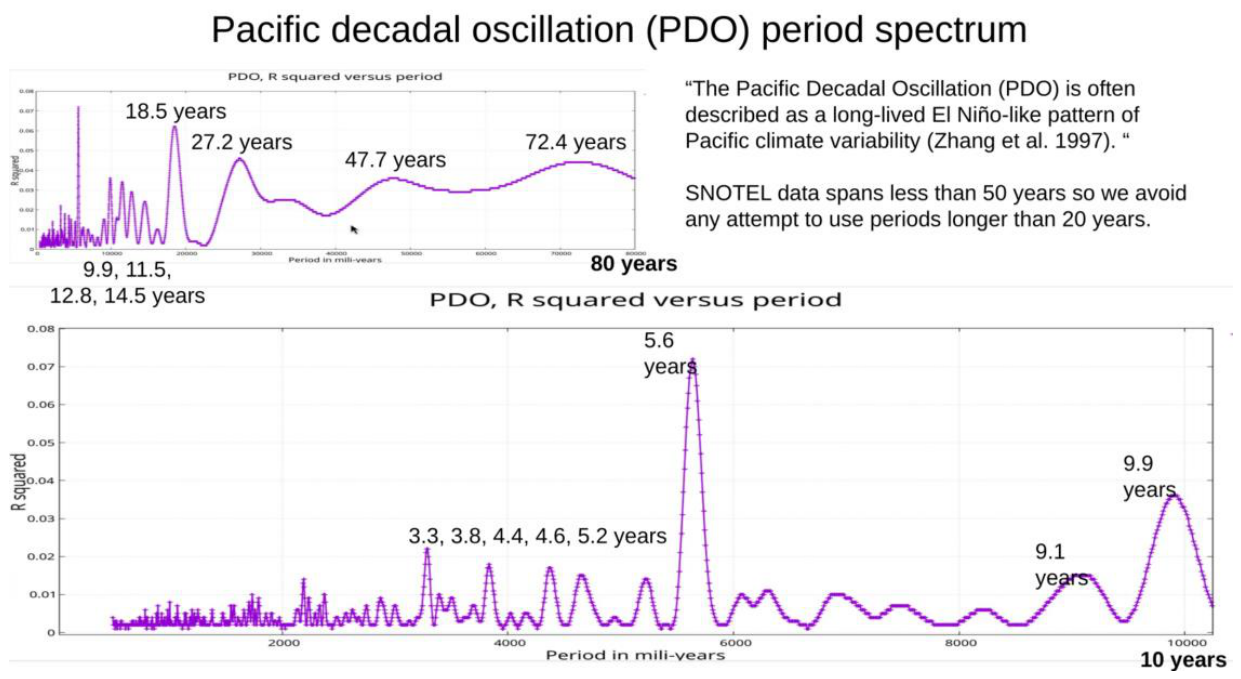
Figure A2.
Pacific/North American Pattern (PNA) period spectrum. Upper left: to 80 years. Upper right: to 20 years. Lower: expanded to 5 years. This index is the noisiest of the five, and its principal peaks fall at shorter periods than those of the other indices.
Figure A2.
Pacific/North American Pattern (PNA) period spectrum. Upper left: to 80 years. Upper right: to 20 years. Lower: expanded to 5 years. This index is the noisiest of the five, and its principal peaks fall at shorter periods than those of the other indices.
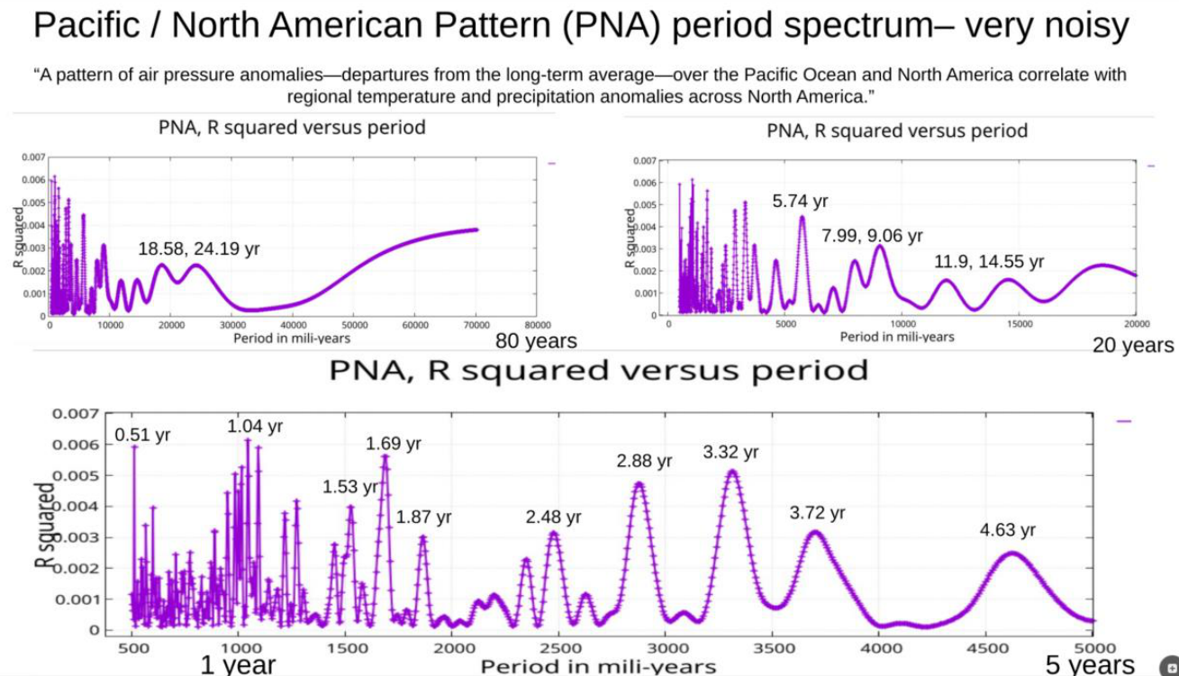
Figure A3.
Atlantic Multidecadal Oscillation (AMO) period spectrum Upper panel: to 80 years. Lower panel: expanded to 20 years.
Figure A3.
Atlantic Multidecadal Oscillation (AMO) period spectrum Upper panel: to 80 years. Lower panel: expanded to 20 years.
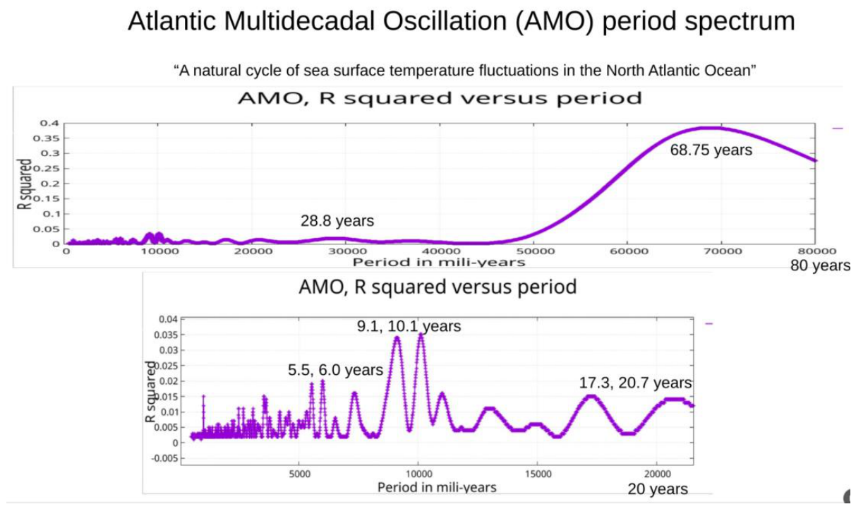
Figure A4.
Southern Oscillation Index (SOI) period spectrum. Upper panel: to 70 years. Lower panel: expanded to 7 years.
Figure A4.
Southern Oscillation Index (SOI) period spectrum. Upper panel: to 70 years. Lower panel: expanded to 7 years.
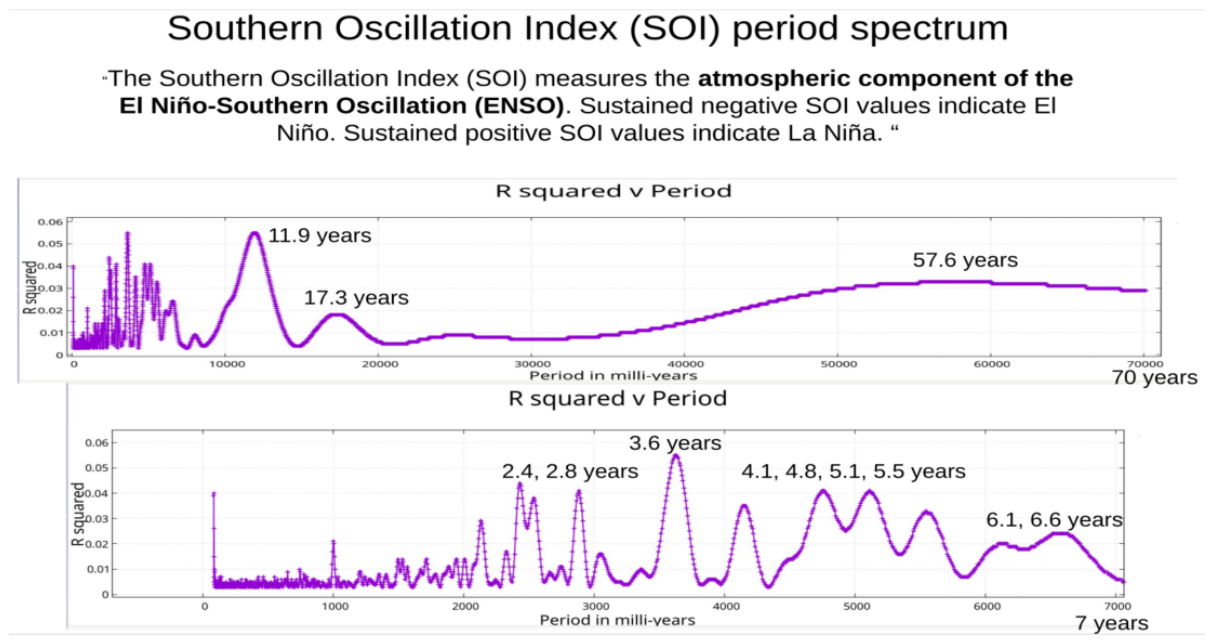
Figure A5.
Total Solar Irradiance (TSI) period spectrum. Upper panel: to 45 years. Lower panel: expanded to 16 years. The 11.3-year peak is the strongest single feature in any of the five spectra.
Figure A5.
Total Solar Irradiance (TSI) period spectrum. Upper panel: to 45 years. Lower panel: expanded to 16 years. The 11.3-year peak is the strongest single feature in any of the five spectra.
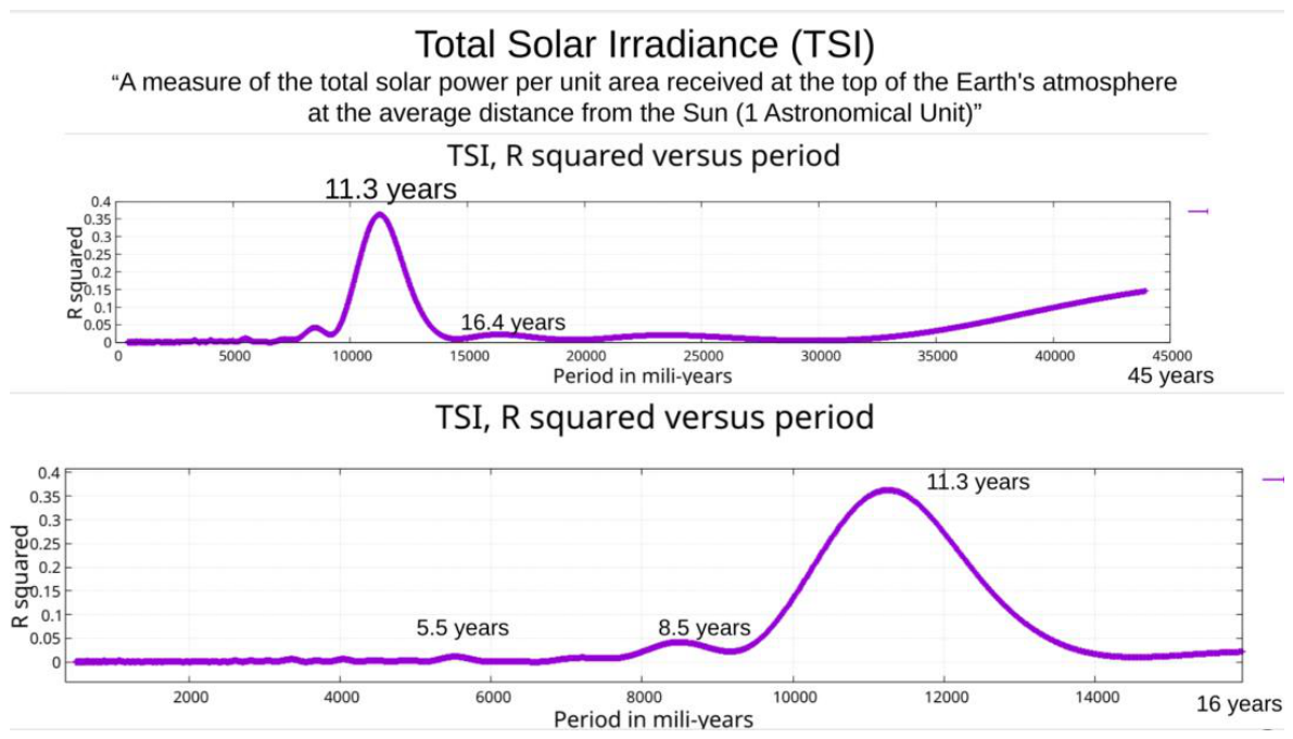
A.2. Composite Spectrum and Band Placement
Figure A6 shows the summed spectrum together with the individual spectra, with the 35 Phase C bands shaded. The sum is formed from the Pacific Decadal Oscillation, Southern Oscillation Index, Atlantic Multidecadal Oscillation and Total Solar Irradiance spectra; the Pacific/North American Pattern is excluded from the sum, although its individual spectrum is used in band selection. The sum is unweighted, so it is dominated by whichever index carries the largest absolute R²: the principal summed peak at 11,360 mY is very largely the Total Solar Irradiance contribution.
Figure A6.
Upper panel: the summed spectrum of the PDO, SOI, AMO and TSI indices, with the 35 Phase C bands shaded. Lower panel: the five individual spectra over the same range, with the vertical scale expanded so the weaker indices are visible; the TSI peak at 11,253 mY reaches R2 = 0.363 and runs off the top of the lower panel
Figure A6.
Upper panel: the summed spectrum of the PDO, SOI, AMO and TSI indices, with the 35 Phase C bands shaded. Lower panel: the five individual spectra over the same range, with the vertical scale expanded so the weaker indices are visible; the TSI peak at 11,253 mY reaches R2 = 0.363 and runs off the top of the lower panel
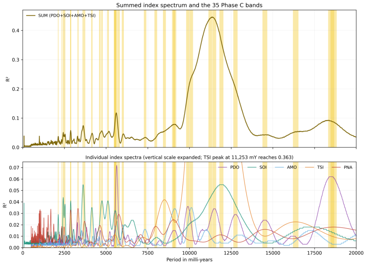
A.3. Provenance of the Phase C Bands
Table A1 matches each of the 35 bands to the nearest peak among the five index spectra. Twenty of the 35 band centres coincide with a peak to the milli-year and 27 fall within 2 mY, which establishes that the bands were read directly from these spectra rather than adopted from published values. The broad bands used in Phases B and D are of different origin and are taken from published periodicities for the ENSO, decadal and solar-cycle ranges; they are not derived from this analysis.
Twenty-three of the 35 bands contain peaks from two or more indices, and several contain peaks from four. Where the resulting bands overlap substantially — the three bands centred at 5,519, 5,545 and 5,546 mY, sourced respectively from the Total Solar Irradiance, Southern Oscillation Index and Atlantic Multidecadal Oscillation spectra, are the clearest case — the redundancy reflects independent detection of the same periodicity by different indices rather than duplicated entries. In search terms such bands act as a single constraint.
Table A1.
Provenance of the 35 narrow precision bands used in Phase C. Each band is matched to the nearest peak, of prominence exceeding 0.0015 in R², among the five index spectra. "Source" is the index whose peak lies closest to the band centre; "also present in" lists other indices whose own peaks fall inside the same band. Half-widths are 1% of the band centre.
Table A1.
Provenance of the 35 narrow precision bands used in Phase C. Each band is matched to the nearest peak, of prominence exceeding 0.0015 in R², among the five index spectra. "Source" is the index whose peak lies closest to the band centre; "also present in" lists other indices whose own peaks fall inside the same band. Half-widths are 1% of the band centre.
| Band centre (mY) | Half-width | Source | Source peak (mY) | R² at peak | Δ (mY) | Also present in |
|---|---|---|---|---|---|---|
| 2134 | ±21 | PDO | 2135 | 0.0060 | 1 | SOI, AMO |
| 2348 | ±23 | PNA | 2348 | 0.0187 | 0 | PDO, SOI |
| 2431 | ±24 | SOI | 2431 | 0.0439 | 0 | AMO |
| 2480 | ±24 | PNA | 2480 | 0.0182 | 0 | PDO, AMO |
| 2533 | ±25 | AMO | 2534 | 0.0040 | 1 | SOI |
| 2876 | ±28 | PNA | 2876 | 0.0330 | 0 | PDO, SOI, AMO |
| 2881 | ±28 | SOI | 2881 | 0.0409 | 0 | PDO, AMO, PNA |
| 3317 | ±33 | PNA | 3317 | 0.0343 | 0 | PDO |
| 3624 | ±36 | SOI | 3626 | 0.0550 | 2 | AMO |
| 3716 | ±37 | PNA | 3716 | 0.0232 | 0 | PDO, TSI |
| 4149 | ±41 | SOI | 4149 | 0.0350 | 0 | PDO |
| 4628 | ±46 | PNA | 4628 | 0.0195 | 0 | PDO, AMO |
| 4755 | ±47 | SOI | 4755 | 0.0410 | 0 | AMO |
| 5115 | ±51 | SOI | 5111 | 0.0410 | 4 | — |
| 5519 | ±55 | TSI | 5520 | 0.0113 | 1 | SOI, AMO |
| 5545 | ±55 | SOI | 5545 | 0.0329 | 0 | AMO, TSI |
| 5546 | ±55 | AMO | 5546 | 0.0190 | 0 | SOI, TSI |
| 5636 | ±56 | PDO | 5636 | 0.0719 | 0 | — |
| 5762 | ±57 | PNA | 5762 | 0.0291 | 0 | — |
| 6005 | ±60 | AMO | 6000 | 0.0200 | 5 | — |
| 7340 | ±73 | AMO | 7335 | 0.0160 | 5 | — |
| 7980 | ±79 | PNA | 7980 | 0.0186 | 0 | SOI |
| 8501 | ±85 | TSI | 8500 | 0.0419 | 1 | — |
| 9040 | ±90 | PNA | 9040 | 0.0244 | 0 | PDO, AMO |
| 9117 | ±91 | AMO | 9117 | 0.0340 | 0 | PNA |
| 9898 | ±98 | PDO | 9904 | 0.0360 | 6 | — |
| 10112 | ±101 | AMO | 10118 | 0.0350 | 6 | — |
| 11252 | ±112 | TSI | 11253 | 0.3629 | 1 | — |
| 11492 | ±114 | PDO | 11498 | 0.0340 | 6 | — |
| 11914 | ±119 | SOI | 11920 | 0.0550 | 6 | PNA |
| 12760 | ±127 | PDO | 12760 | 0.0290 | 0 | — |
| 14524 | ±145 | PNA | 14524 | 0.0160 | 0 | PDO |
| 16370 | ±163 | TSI | 16369 | 0.0226 | 1 | — |
| 18500 | ±185 | PDO | 18492 | 0.0620 | 8 | PNA |
| 18644 | ±186 | PNA | 18644 | 0.0180 | 0 | PDO |
By primary source, the bands divide as: Pacific/North American Pattern 11, Southern Oscillation Index 8, Pacific Decadal Oscillation 6, Atlantic Multidecadal Oscillation 6, and Total Solar Irradiance 4.
Appendix B. Example Site Report — SNOTEL 1030 Arapaho Ridge, Colorado
To illustrate the validation process and output format, this appendix reproduces key sections from the formal site characterization report for SNOTEL 1030 (Arapaho Ridge, Colorado), a Tier I site in the Never Summer Mountains, Grand County, Colorado.
This site is unchanged by the peak-assignment correction. Under both PD1 and PD3.1 its pass rate is 93.3%, winning configuration 2p/FNCA_0.20/B, Tier I, ValueCV 0.087, STBL, reliability score 92.6. Every reported quantity is identical. As an interior Colorado station it has no December-dominant accumulation years, so the water-year reassignment has nothing to act on — which is what Section 3.5 predicts and a useful illustration of the correction's selectivity. The Version 2 site report therefore stands without revision.
Prediction Grading Scale
Predictions are graded on an academic scale based on the ratio of predicted peak SWE to observed peak SWE, expressed as a percentage. A ratio of 100% indicates a perfect prediction. Over-prediction is penalized more harshly than under-prediction because shortage destroys client trust and creates operational emergencies for water managers. Over-prediction enters the failing range at +27% deviation; under-prediction fails at −31% deviation. A grade of C− or better constitutes a pass. Grading is performed entirely by software with no human intervention.
Table B1.
Full asymmetric grading scale.
| Grade | Over-prediction (pred/obs) | Under-prediction (pred/obs) | Result |
|---|---|---|---|
| A+ | 100–102% | 97–99% | Pass |
| A | 103–105% | 94–96% | Pass |
| A− | 106–108% | 90–93% | Pass |
| B+ | 109–111% | 87–89% | Pass |
| B | 112–114% | 84–86% | Pass |
| B− | 115–117% | 80–83% | Pass |
| C+ | 118–120% | 77–79% | Pass |
| C | 121–123% | 74–76% | Pass |
| C− | 124–126% | 70–73% | Pass (threshold) |
| D+ | 127–129% | 67–69% | Fail |
| D | 130–132% | 64–66% | Fail |
| D− | 133–135% | 60–63% | Fail |
| F | ≥136% | <60% | Fail |
Figure B1.
SNOTEL 1030 Arapaho Ridge: full record overview. Purple: observed SWE. Green: model fit and extrapolation. Blue: measured data beyond the training cutoff.
Figure B1.
SNOTEL 1030 Arapaho Ridge: full record overview. Purple: observed SWE. Green: model fit and extrapolation. Blue: measured data beyond the training cutoff.
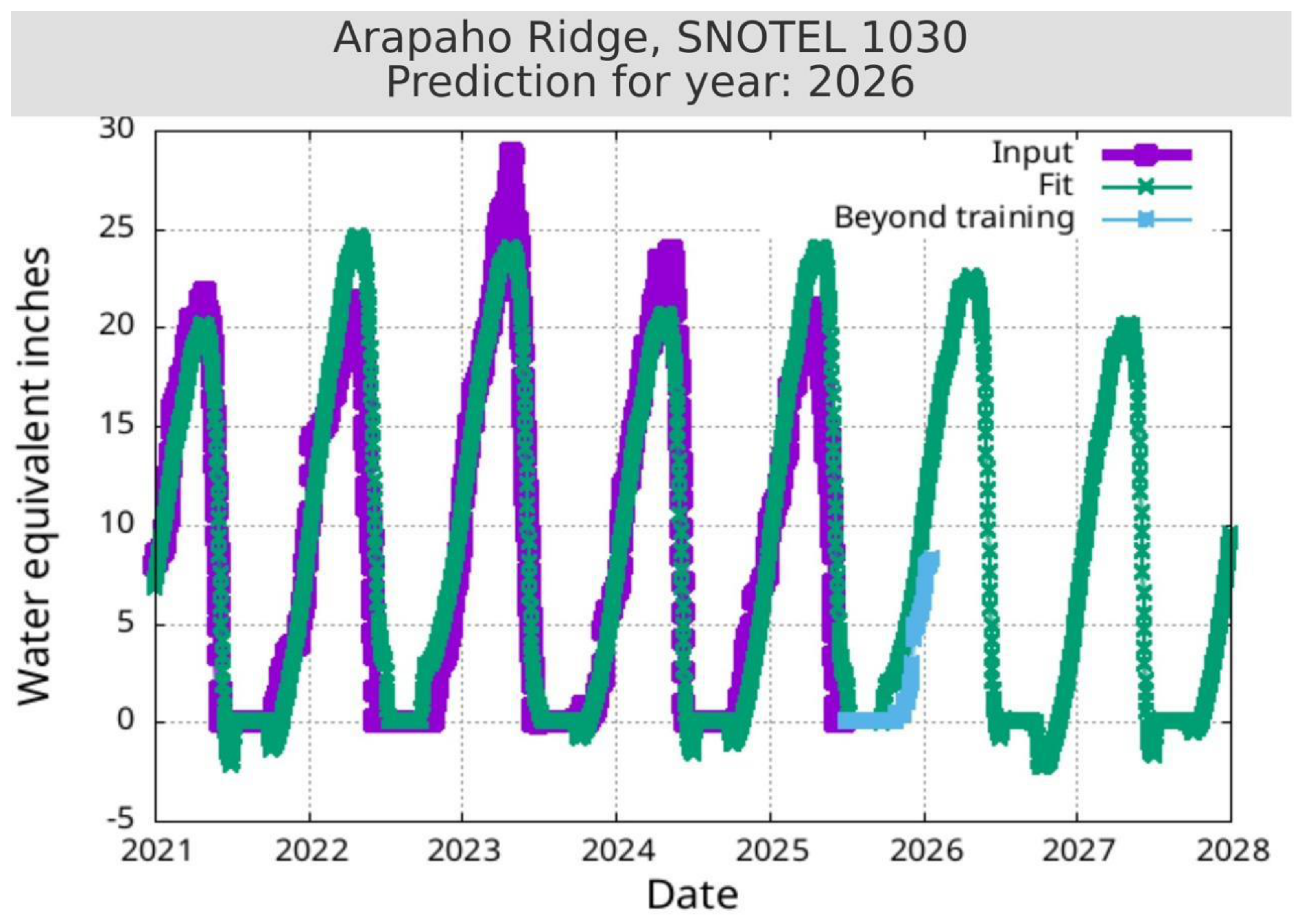
Snowless water years. A water year whose observed peak SWE is zero is not scored by this ratio. It is graded as a failure when the model predicts non-zero accumulation. Years with small but non-zero observed peaks are scored normally by the table above.
Appendix B.1. Site Overview
SNOTEL station 1030 at Arapaho Ridge sits at 10,960 ft in Grand County, Colorado. The station has recorded continuous snowpack data since 2002, providing over two decades of SWE measurements. Snowmelt from the Arapaho Ridge area contributes to both the Colorado River Headwaters and Willow Creek, positioning the station's data as relevant to water supply planning for downstream communities dependent on spring runoff from the Never Summer Mountains.
| Station name | Arapaho Ridge |
|---|---|
| SNOTEL number | 1030 |
| Elevation | 10,960 ft (3,340 m) |
| Location | 40°21′N, 106°22′W |
| County | Grand County, Colorado |
| HUC basin | Rabbit Ears Creek–Troublesome Creek |
| Data record | 2002–present |
| Operating agency | NRCS |
Appendix B.2. Validation Results
Arapaho Ridge achieves a 93.3% pass rate across 15 graded holdout years, earning a Tier I rating. One failure occurs across the record, prediction year 2012. Signal analysis indicates high consistency in the underlying climate signals detected at this site, with a reliability score of 92.6 out of 100.
Table B2.
Grade distribution across 15 graded holdout years.
| Grade range | A+/A/A− | B+/B/B− | C+/C/C− | D+/D/D− | F |
|---|---|---|---|---|---|
| Count | 6 | 4 | 4 | 0 | 1 |
| Result | Pass | Pass | Pass | Fail | Fail |
Fourteen of fifteen predictions grade at C− or better. A+ grades in 2015 and 2017 demonstrate near-exact predictions, and the model shows particular strength in the later record with eleven consecutive passing grades from 2013 through 2025.
Table B3.
Year-by-year prediction grades. Years shown are predicted years, one beyond each holdout cutoff.
Table B3.
Year-by-year prediction grades. Years shown are predicted years, one beyond each holdout cutoff.
| Year | Grade | Status | Year | Grade | Status |
|---|---|---|---|---|---|
| 2009 | A− | Pass | 2018 | P | Plot-only |
| 2010 | B | Pass | 2019 | B+ | Pass |
| 2011 | C− | Pass | 2020 | A− | Pass |
| 2012 | F | Fail | 2021 | A− | Pass |
| 2013 | A | Pass | 2022 | C− | Pass |
| 2014 | C+ | Pass | 2023 | P | Plot-only |
| 2015 | A+ | Pass | 2024 | B | Pass |
| 2016 | B− | Pass | 2025 | C− | Pass |
| 2017 | A+ | Pass | 2026 | P | Plot-only |
Plot-only (P) years are computed and plotted but excluded from the pass rate. 2018: warm snow drought. 2023: Hunga Tonga forcing period. 2026: warm snow drought, outside scope (Section 5.6).
Appendix B.3. Algorithm Characteristics
The system uses a greedy search with mathematical constraints to prevent overfitting, testing model configurations of varying complexity and selecting the simplest model achieving the highest prediction accuracy on held-out data. This reflects the well-established statistical principle that parsimonious models often extrapolate better than complex ones, even when the complex model fits the training data more closely.
The algorithm's fit quality is intentionally moderate — typical R² values of 0.15–0.35 against cross-validated data, after removal of a typical year's snowfall before fitting. This may seem low compared with models reporting R² against their own training data, but it reflects honest out-of-sample performance. The system captures the periodic component of snowpack variation while accepting that weather-scale stochastic variation is inherently unpredictable at the one-year horizon. The useful output is not a precise SWE value but a graded forecast: whether the coming year will be above-normal, near-normal, or below-normal relative to the site's climatology.
Appendix B.4. Prediction Scope and Limitations
The system predicts site-specific one-year-ahead peak SWE using periodic climate signals. It does not predict, and should not be relied upon to predict, the following.
Future volcanic eruptions. The system incorporates the effects of past eruptions but has no capacity to anticipate future ones. An eruption comparable to Pinatubo would produce a forcing outside the model's scope.
Unprecedented drought or precipitation extremes. The harmonic model captures the frequency of ENSO oscillations but not the extreme amplitude of rare events. Seasons such as 2010–2011, when an unusually strong La Niña produced record-low snowpack across much of the West, involve amplitudes exceeding the model's calibrated range.
Warm snow drought events. The 2018 and 2026 seasons demonstrate a failure mode in which anomalous warmth causes precipitation to fall as rain rather than snow, reducing snowpack without reducing total precipitation. This is outside scope by construction (Section 5.8).
Single-storm or sub-seasonal events. The system operates at the annual timescale and does not predict individual storms, atmospheric rivers, or melt-onset timing within a season.
Within its designed scope, the system provides objective, reproducible forecasts validated against the full historical record at each site. When a water manager recognizes that an anomalous forcing event is building, the forecast for that year can be compared against a matching event in the site's own prediction history; some sites are strongly affected by anomalous events while others show little change.
Appendix C. Configuration Search Order
Each phase tests the following configurations in order, stopping at early-exit conditions:
1p/FNCA_0.40 · 2p/FNCA_0.20 · 2p/FNCA_0.10 · 2p/FNCA_0.05 · 2p/FNCA_0.02 · 3p/FNCA_0.20 · 3p/FNCA_0.10 · 3p/FNCA_0.05 · 4p/FNCA_0.20 · 4p/FNCA_0.10 · 4p/FNCA_0.05
Here np is the number of harmonic periods and FNCA the overfitting constraint threshold; lower FNCA means a tighter orthogonality requirement. Configurations are tested from simplest to most complex, and from tightest to loosest FNCA at each period count. The search terminates at four periods.
Appendix D. Changes From Version 2
Appendix D.1. What ChangedAppendix D.2. What Did Not Change
| Item | Version 2 | Version 3 |
|---|---|---|
| Peak-to-year assignment | Calendar year | Water year (§2.3) |
| Snowless water years | Scored as perfect | Scored as failure when model predicts snow |
| Grader | PD1 | PD3.1 |
| ≥15-year record rule | Stated, not enforced | Enforced; 61 stations excluded (§2.1) |
| Montana | 88.4% | 87.2% |
| Colorado | 86.4% | 86.3% |
| Wyoming | 84.2% | 84.1% |
| Idaho | 83.3% | 81.8% |
| Washington | 81.5%, grouped above 80% | 76.0%, below operational average |
| Utah | 75.5% | 75.4% |
| Oregon | 70.8% | 65.7% |
| California | 49.3% | 44.3%, no qualifying station |
| Oregon STBL sites | 75.5% | 68.5% |
| Washington STBL sites | 88.6% | 84.9% |
| Two-year roster | 220 | 206 |
| 2026 decomposition baselines | Mixed: 18-yr SWE vs full-record precipitation | Full-record split-half for both |
| 2026 decomposition shares | 18 / 29 / 53 | 9 / 40 / 51 |
| 2026 peak-timing channel | Not reported | Reported (Table 15) |
| Cascade east–west split | Attributed to rain shadow | Largely an elevation contrast (§5.7) |
| Geographic predictor | Pattern stability, per 15-site pilot | Elevation dominant; measured on 622 stations |
| Annual-cycle stationarity | Not reported | Measured; Pacific states least stable (Table 11) |
| Holdout/prediction offset | Not stated | Stated (§2.8) |
| Record-length gates | Not stated | Stated and enforced (§2.1, §2.8) |
| Baseline fixed across holdouts | Not stated | Stated with rationale (§2.2) |
| Seasonal mask construction | Not described | Described with rationale (§2.2) |
| VCV provenance | Not stated | Stated (§2.9) |
| Period complexity table | Not reproducible; impossible caption | Recomputed and defined (§4.6) |
| Phase win claim | "Phase D wins in all three primary states" | Corrected: Phase B in Colorado (§4.7) |
The frqsrchX algorithm, the FNCA constraint, the MASK band definitions, the volcanic impulse framework, the five-phase pipeline, the configuration search order, the grading scale, the tier thresholds, and the reliability score formula are all unchanged. The input SWE records are the same vintage used for Versions 1 and 2. The three commercially targeted interior states are confirmed essentially unchanged in aggregate performance. The 2026 event remains outside scope, the historical validation window remains unaffected by it, and the 2027 forecasts generated during the 2025 model run stand without revision.
Appendix D.3. Station Roster Differences and a Recovered Output Defect
Six stations present in Version 2 were initially missing from the Version 3 state summaries: 675 Overland Res. (CO), 492 Garfield R.S. (ID), 679 Paradise and 910 Elbow Lake (WA), 1114 Garden City Summit (UT), and 539 Independence Camp (CA). They are not station retirements and their absence had nothing to do with the peak-assignment correction.
All six were characterized normally. Each produced a complete text characterization report carrying its recommendation block, and a complete score sidecar carrying its winning configuration, pass rate, period-stability value and reliability score. What failed in each case was a single page of the presentation artifact that the period-collection stage reads: the title slide, which carries the site name, winning configuration and pass rate, was written empty. The collection stage identifies sites by reading exactly those fields from that page, so it treated each of these six as producing no usable data and dropped them without a diagnostic. The loss then propagated to the stability table and to the state summary.
The defect is detectable directly — a characterization presentation lacking a Best Pass Rate: field is incomplete by construction — and a check to that effect now gates the pipeline. Applied across all eight states it identified exactly these six files and no others, and the resulting counts reconcile against every state summary without residual. The recovered values are taken from the score sidecars, which are authoritative for all quantities reported here.
Table D1.
Recovered stations.
| Station | PD1 | PD3.1 | Δ (pp) |
|---|---|---|---|
| 675 Overland Res., CO | 80.0% · II · STBL | 80.0% · II · STBL | 0.0 |
| 492 Garfield R.S., ID | 66.6% · III | 66.6% · III | 0.0 |
| 679 Paradise, WA | 100.0% · I · STBL | 93.3% · I · STBL | −6.7 |
| 910 Elbow Lake, WA | 73.3% · III | 73.3% · III | 0.0 |
| 1114 Garden City Summit, UT | 76.9% · II | 76.9% · II | 0.0 |
| 539 Independence Camp, CA | 60.0% · III | 53.3% · III | −6.7 |
Stability classes are shown only for stations clearing the 80% score gate, where the slot-based value is authoritative (Section 2.9); for the remainder the reported class derives from the row-position value and is not reproduced here. Only 679 changes the two-year roster, which it rejoins as a Tier I stable site.
The two stations that moved are both maritime, and both moved down by the same 6.7 points — consistent with the gradient of Section 3.4 rather than an independent effect. Station 679 is the more striking of the two: a site with a perfect fifteen-of-fifteen record under the original grader, an unchanged winning configuration, and one of the most stable period selections in the network, which nonetheless loses a holdout once its December-dominant water year is graded against the correct prediction.
After recovery, the remaining roster differences from Version 2 are additions only, reflecting the state of the NRCS network at the time of the re-run:
| State | Added in Version 3 |
|---|---|
| Colorado | 345 Bison Lake; 1324, 1325, 1326, 1344 (no fit produced) |
| Montana | 858; 1322 (no fit produced) |
| Wyoming | 818 |
| Washington | 791 Stevens Pass |
| California | 1331, SNOW SENSORS TES (no fit produced) |
Appendix D.4. Two Further Roster Corrections
Ungraded sites in the Version 2 Utah baseline. Ten stations across the network are too recently installed to support a fit; they return the default single-period configuration with no period record and no stability classification, and are excluded from the results here. Two of them — 1321 Mill Creek Canyon and 1323 Elk Ridge, at 6.6% and 0.0% — were present in the Utah roster used for Version 2 and were counted in its state average. Removing them raises the Version 2 Utah baseline from 75.5% to 76.8%, and the corrected Version 3 figure is 76.5%. The Version 2 Utah average was therefore depressed by roughly 1.3 percentage points for a reason unrelated to the grader, and the state's apparent improvement between versions is an artifact of that correction rather than an effect of the water-year reassignment. Utah's grader-driven change, measured on a consistent roster, remains −0.34 points. The other eight ungraded sites postdate Version 2 and affect no published figure. Wyoming's roster likewise falls from 88 to 87 on this rule, raising its Version 3 average from 83.5% to 84.1%.
Stability records recovered from a display-name join defect. Four stations carry a display name whose two-letter state suffix loses its final character in the text extracted from the summary presentation — 311 Banfield Mountain and 667 North Fork Jocko in Montana, and 333 Ben Lomond Trail and 435 Daniels-Strawberry in Utah. The stability table is joined on the full display name, so these four failed the join and initially carried no stability classification, though their pass rates, tiers and period records were complete and their records span 36 to 48 years. Their classifications have been recovered from the stability output directly and are included in the results reported here: 311 and 667 are stable and Tier I and both qualify for the two-year roster; 333 is unstable and 435 stable, both Tier III. A fifth station, 1215 Lasal Mountain Lower, also lacks a stability classification, but for an unrelated and correct reason: its record spans 13.3 years, so it fails the fifteen-year requirement of Section 2.1 and no holdout attains the fifteen-year training span the stability metric requires. The join defect is present in both the Version 2 and Version 3 runs and is independent of the peak-assignment correction. It is avoided by keying the join on the site identifier that precedes the colon in the display name, which is immune to the loss of a trailing character and distinguishes SNOTEL from SNOW SENSOR stations without ambiguity.
Appendix D.5. A Defect in Holdout Truncation, and Its Effect on California
Thirty-two California stations produced no viable fit in the initial Version 3 runs. The cause was in the step that truncates a station's record at the holdout cutoff before the fit is performed.
That step located the cutoff by searching the input file for the literal text of the mid-season date, using a line editor. The search assumes a sample exists at that date. SNOW SENSOR stations report seasonally, and many carry summer gaps where the record passes from spring melt-out directly to the following autumn with no intervening entries. At an affected station the searched-for date was simply not present in the file, the search failed, and the truncation removed the entire record rather than the intended tail. The period search then received an empty file and reported a maximum search period of zero — below its minimum — so that no candidate period was ever tested and no fit could be produced.
The failure is therefore keyed to summer reporting behaviour, which is why it presented almost exclusively at SNOW SENSOR sites (31 of 32) while SNOTEL stations, which report year-round, were nearly untouched. It is unrelated to record length: the affected stations include sites with forty years of data.
The search has been replaced with a Fortran routine that performs a numeric comparison, retaining samples at or before the cutoff. This requires no sample to exist at the boundary and is insensitive to gaps of any length.
The effect on results was to suppress roughly a third of each affected station's holdouts, which were then scored as prediction failures under the rule of Section 2.8. After repair those stations recovered a mean of 7.8 percentage points and three holdouts each at the median, and California's state average rose from 42.3% to 44.3%.
Two consequences for figures reported elsewhere. California's correction magnitude in Table 2 is −4.10 points measured on repaired data; a figure of −6.21 computed beforehand conflated the grader change with this defect and should not be used. And the correction magnitude is not monotonic across all eight states once California is measured correctly — the three Pacific states cluster without a meaningful internal ordering (Section 3.4).
Appendix D.6. Reporting-Layer Repairs
Three defects in the summary-extraction utility were identified and fixed during this work. None altered a computed value; all were display or parsing issues affecting how results were written out, not how they were graded. They are: a display inconsistency in which tabular output printed one VCV provenance while the derived stability class used another; a site-recognition regression that dropped SNOW SENSOR stations from California summaries; and a period-parsing defect that injected duplicate period entries at two stations network-wide. A mutation-tested regression harness now gates the utility against all three.
References
- Higginbotham, J. Climate, Water Vapor, and Volcanic Eruptions. Env. Sci. Clim. Res. 4(1), 01–09. [CrossRef]
- Higginbotham, J. Antarctic Ice Core Harmonic Analysis. Env. Sci. Clim. Res. 2026b, 4(1), 01–24. [Google Scholar] [CrossRef]
- NRCS. SNOTEL Network Data. Natural Resources Conservation Service, USDA. 2025. Available online: https://wcc.sc.egov.usda.gov/reportGenerator/.
- Barnston, A. G.; Livezey, R. E. Classification, seasonality and persistence of low-frequency atmospheric circulation patterns. Mon. Wea. Rev. 1987, 115, 1083–1126. [Google Scholar] [CrossRef]
- Dettinger, M. D.; Cayan, D. R.; Diaz, H. F.; Meko, D. M. North–south precipitation patterns in western North America on interannual-to-decadal timescales. J. Clim. 1998, 11, 3095–3111. [Google Scholar] [CrossRef]
- Mantua, N. J.; Hare, S. R.; Zhang, Y.; Wallace, J. M.; Francis, R. C. A Pacific interdecadal climate oscillation with impacts on salmon production. Bull. Amer. Meteor. Soc. 1997, 78, 1069–1079. [Google Scholar] [CrossRef]
- Cayan, D. R. Interannual climate variability and snowpack in the western United States. J. Clim. 1996, 9, 928–948. [Google Scholar] [CrossRef]
- Trenberth, K. E. The definition of El Niño. Bull. Amer. Meteor. Soc. 1997, 78, 2771–2777. [Google Scholar] [CrossRef]
- Mote, P. W.; Hamlet, A. F.; Clark, M. P.; Lettenmaier, D. P. Declining mountain snowpack in western North America. Bull. Amer. Meteor. Soc. 2005, 86, 39–49. [Google Scholar] [CrossRef]
- Dettinger, M. D. Climate change, atmospheric rivers, and floods in California — A multimodel analysis of storm frequency and magnitude changes. J. Amer. Water Resour. Assoc. 2011, 47, 514–523. [Google Scholar] [CrossRef]
- Higginbotham, J. Integrated Category Analysis; Walker Water LLC, 2025. [Google Scholar]
Figure 1.
This is an example where fifteen cases of truncated input data successfully predicted peak water equivalent one year beyond. Here the method is applied to predict 2026 peak water equivalent.
Figure 1.
This is an example where fifteen cases of truncated input data successfully predicted peak water equivalent one year beyond. Here the method is applied to predict 2026 peak water equivalent.
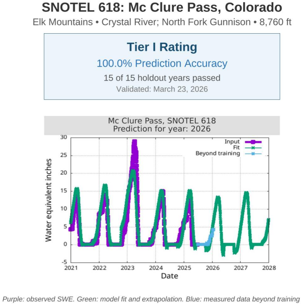
Figure 2.
The input data is divided into the early half and late half. These halves are averaged. Then the average for a given year is found by linearly interpolation between these halves.
Figure 2.
The input data is divided into the early half and late half. These halves are averaged. Then the average for a given year is found by linearly interpolation between these halves.
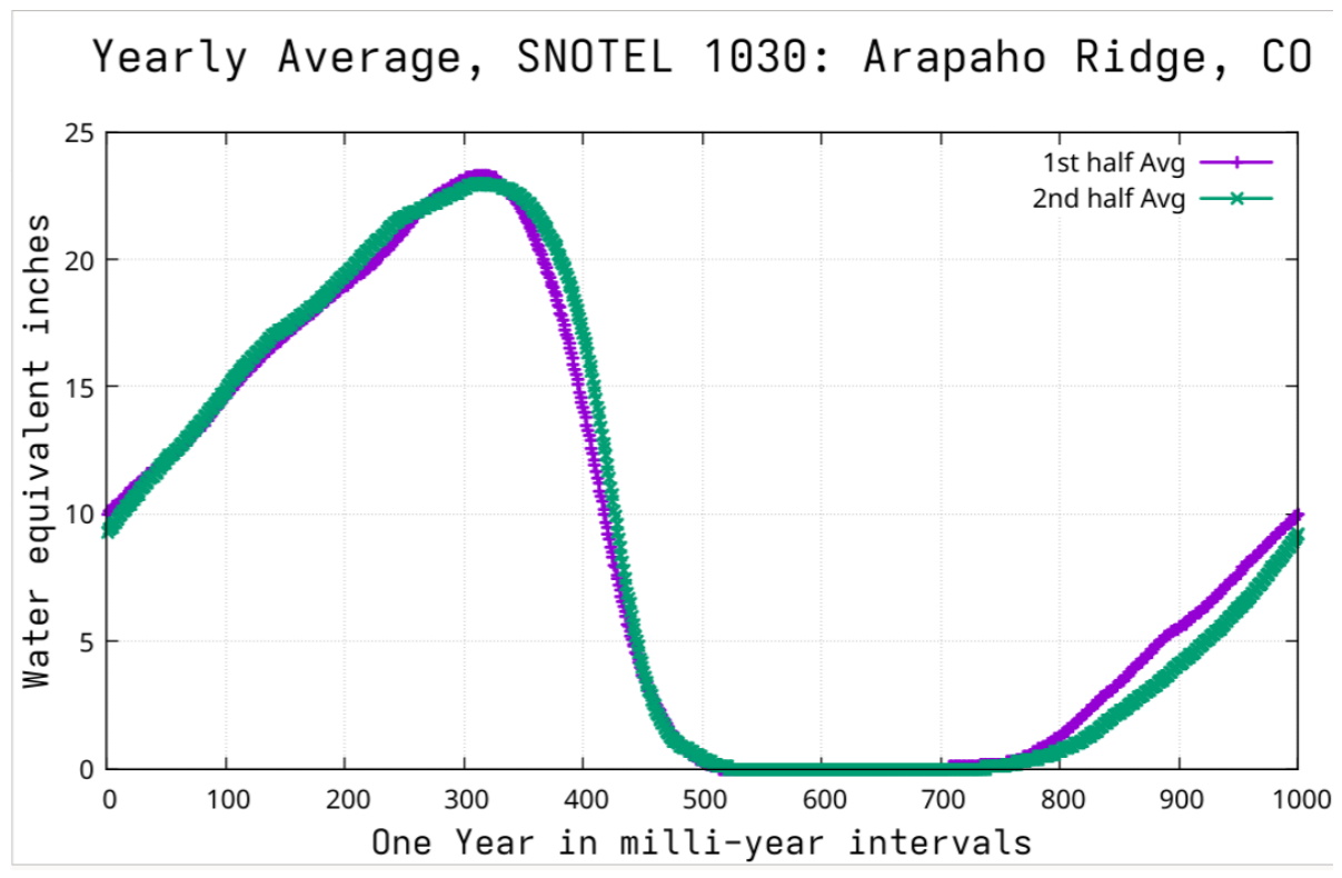
Figure 3.
Residual following subtraction of average. The fit is done on this residual and the average is then added back in. Note: the strong peaks and troughs of this figure are NOT at the peak time of year seen in Figure 2. The noisy nature of this residual means that the is not expected to be high when a limited number of periods are involved in the fit.
Figure 3.
Residual following subtraction of average. The fit is done on this residual and the average is then added back in. Note: the strong peaks and troughs of this figure are NOT at the peak time of year seen in Figure 2. The noisy nature of this residual means that the is not expected to be high when a limited number of periods are involved in the fit.
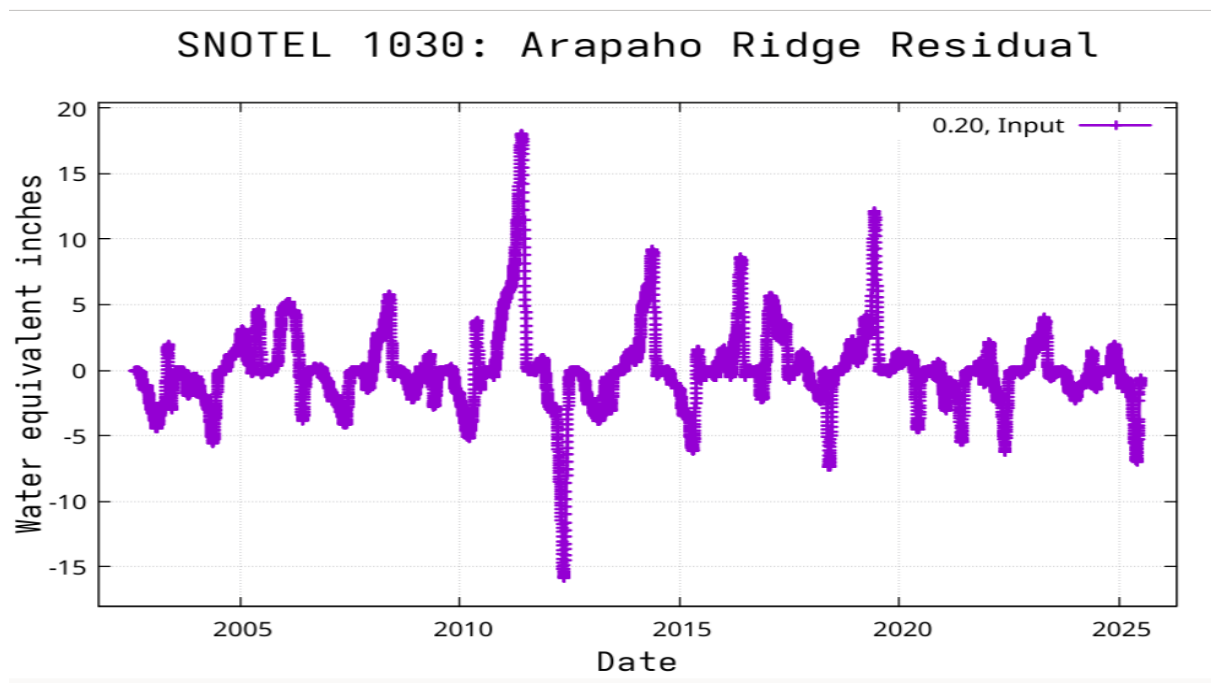
Figure 4.
Here Atmospheric Transmission is fit using a constant, fifteen periods, and 23 impulse functions for volcanic eruptions.
Figure 4.
Here Atmospheric Transmission is fit using a constant, fifteen periods, and 23 impulse functions for volcanic eruptions.
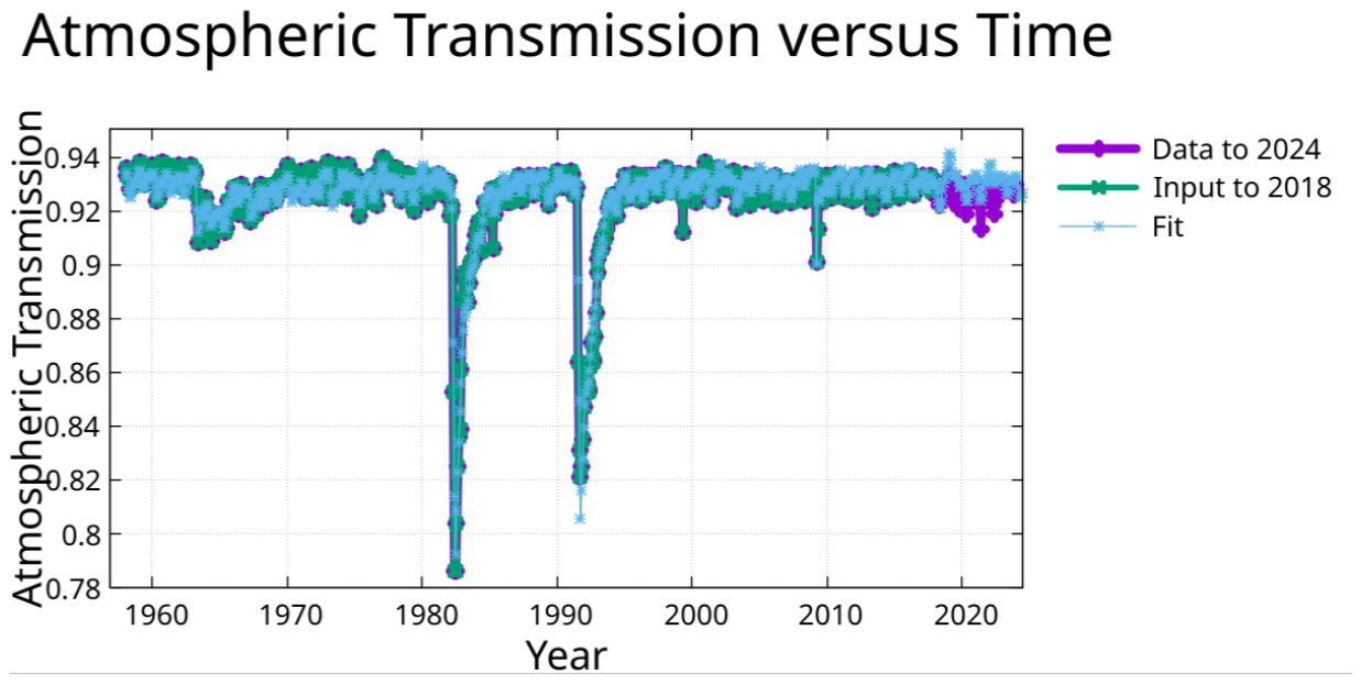
Table 6.
Period complexity of winning configurations (PD3.1, all graded sites). Percentages are of sites whose winning configuration uses each period count, and sum to 100%.
Table 6.
Period complexity of winning configurations (PD3.1, all graded sites). Percentages are of sites whose winning configuration uses each period count, and sum to 100%.
| State | 1-period | 2-period | 3-period | 4-period |
|---|---|---|---|---|
| Colorado | 15.9% | 52.2% | 20.4% | 11.5% |
| Montana | 17.9% | 40.0% | 24.2% | 17.9% |
| Wyoming | 13.6% | 43.2% | 29.5% | 13.6% |
Table 9.
Seven-state 2026 prospective outcome by state, graded under the corrected routine.
| State | Sites | 2026 F-rate | Median pred/obs | Mean peak-date error |
|---|---|---|---|---|
| Oregon | 81 | 98.8% | 294% | −30.0 d |
| Colorado | 117 | 93.2% | 169% | −23.2 d |
| Utah | 112 | 92.9% | 212% | −23.4 d |
| Washington | 75 | 69.3% | 177% | −17.6 d |
| Idaho | 83 | 54.2% | 139% | −13.7 d |
| Wyoming | 84 | 52.4% | 137% | −18.4 d |
| Montana | 95 | 35.8% | 123% | −11.1 d |
Table 10.
Correlation of pass rate with station geography, by state (Pearson r).
| State | Elevation | Latitude | Longitude | Mean elevation |
|---|---|---|---|---|
| Washington | +0.543 | +0.211 | +0.043 | 4,330 ft |
| Oregon | +0.511 | +0.200 | +0.423 | 4,940 ft |
| Montana | +0.386 | −0.195 | −0.224 | 6,865 ft |
| Utah | +0.301 | +0.353 | +0.428 | 8,603 ft |
| Wyoming | +0.232 | −0.128 | +0.171 | 8,627 ft |
| Idaho | +0.094 | +0.325 | +0.012 | 6,475 ft |
| California | −0.021 | +0.300 | −0.339 | 7,703 ft |
| Colorado | −0.098 | +0.221 | −0.090 | 10,133 ft |
| Pooled within-state | +0.294 |
Disclaimer/Publisher’s Note: The statements, opinions and data contained in all publications are solely those of the individual author(s) and contributor(s) and not of MDPI and/or the editor(s). MDPI and/or the editor(s) disclaim responsibility for any injury to people or property resulting from any ideas, methods, instructions or products referred to in the content. |
© 2026 by the authors. Licensee MDPI, Basel, Switzerland. This article is an open access article distributed under the terms and conditions of the Creative Commons Attribution (CC BY) license (http://creativecommons.org/licenses/by/4.0/).
Copyright: This open access article is published under a Creative Commons CC BY 4.0 license, which permit the free download, distribution, and reuse, provided that the author and preprint are cited in any reuse.