On the Hitting Time Index of Broom Graphs

1. Introduction

A finite simple connected undirected graph $G=(V,E)$ with vertex set $V=\{1,2,\dots ,n\}$ and edge set E is used in Mathematical Chemistry to model a molecule, taking the vertices as the atoms, and the edges as the atomic bonds. Reference [1] contains all the graph theoretical concepts needed in what follows.

On such graphs, many molecular indices, or descriptors, i. e., real-valued functions on the domain of all graphs, have been put forward in order to identify physico-chemical properties of the molecules and to classify them according to the values of their indices. One such index is the hitting time index, first introduced in [6], which is based on the behavior of the simple random walk on G. This random walk is defined as the Markov chain $\{X_n,n\ge 0\}$ with state space V and uniform transition probabilities ${\displaystyle \frac{1}{d_i}}$ from a vertex i to any of its $d_i$ neighboring vertices. The hitting time $T_j$ of the vertex j is defined as the smallest number of steps needed by the random walk to hit the vertex j:

$$T_j=inf\{n\ge 0:X_n=j\},$$

and its expected value, when the random walk starts in state i is denoted by $E_i{T}_j$. Let it be noted that $E_i{T}_i=0$, and this should not be confused with the mean return time to vertex i, $E_i{T}_i^{+}={\displaystyle \frac{2\left|E\right|}{d_i}}$, which involves $T_i^{+}=inf\{n\ge 1:X_n=i\}$. For all details involving hitting times of Markov chains, one may look at reference [3].

We can define now the hitting time index of a graph G, $HT\left(G\right)$, as

$$HT\left(G\right)=\sum _{i<j}D(i,j),$$

where $D(i,j)=max\{E_i{T}_j,E_j{T}_i\}$.

We studied the $HT$ index in a series of articles ([6,7,8]), finding relationships between this new index and other important indices, as well as some closed-form formulas for the values of the index for families of graphs endowed with some symmetries. More recently, He et al. found in [5] a number of new results for the $HT$ index, among them a formula for the value of the index of some broom graphs $B_{n,d}$, defined as a graph with n vertices, made up of a path $P_d$ with d vertices and $(n-d)$ pendant vertices attached to one of the ends of the path $P_d$. Specifically, they found that for $n\ge 8$ and $4\le d\le {\displaystyle \frac{n}{2}}$ one has

$$HT\left(B_{n,d}\right)=\sum _{1\le i<j\le d}(j-i)(2n-j-i)+\sum _{1\le i\le \lfloor {\displaystyle \frac{(n+1)-\sqrt{\Delta }}{2}}\rfloor }(n-d)(d-i)(2n-d-i)$$

$$+\sum _{\lfloor {\displaystyle \frac{(n+1)-\sqrt{\Delta }}{2}}\rfloor }(n-d)(d-i+1)(d+i-1)$$

$$(n-d)\left(n^2-2d^2+dn-d-2+\lfloor {\displaystyle \frac{(n+1)-\sqrt{\Delta }}{2}}\rfloor (2d-2n+3)\right),$$

where $\Delta =4d^2+n^2-4nd+6n-4d+9$.

This calculation for $HT\left(B_{n,d}\right)$ was carried out using the characterization of hitting times in terms of voltages, when the graph is considered as an electric circuit where all the edges have unit resistance. The result shows how complicated the expression of the value for this index can be, even for a deceptively simple graph. In this article, instead of voltages we use the commute time formula for a random walk on a graph (which in essence depends on the effective resistance), and find reasonably simpler expressions for $HT\left(B_{n,d}\right)$ when $d=n-2$ and $n\ge 5$; $d=3$ and $n\ge 6$; $d=4$ and $n\ge 7$, and suggest how to obtain other similar expressions for other cases, some of which are not covered in [5].

2. The Results

There is a close relationship between random walks on graphs and electric networks, spelled out in reference [4]. An important result in this context, that was proved in [2], is the formula for the commute time given in the following lemma.

Lemma 1.

For any $i,j\in G$ we have

$$E_i{T}_j+E_j{T}_i=2\left|E\right|R_{ij},$$

(1)

where $R_{ij}$ is the effective resistance between vertices i and j when the graph is considered as an electric network where all the edges are unit resistors.

An immediate corollary of (1) is that if $i,j\in G$ and G is a tree, then

$$E_i{T}_j+E_j{T}_i=2(n-1)d(i,j)$$

(2)

where $d(i,j)$ is the distance (length of a shortest path) between i and j.

In [6] we showed the following result that will be used below.

Lemma 2.

For the path graph $P_n$ on n vertices we have

$$HT\left(P_n\right)=\sum _{k=1}^{\lfloor {\displaystyle \frac{n}{2}}\rfloor }\sum _{m=k+1}^{n-k+1}(2n-m-k)(m-k)+\sum _{k=\lfloor {\displaystyle \frac{n}{2}}\rfloor +2}^n\sum _{m=n-k+2}^{k-1}(m+k-2)(k-m).$$

(3)

For the following proposition, we denote with a superscript * all quantities related to the path graph $P_n$. Thus, the expected hitting times in the path graph will be denoted by $E_i{T}_j^{*}$, and $D^{*}(i,j)=max\{E_i{T}_j^{*},E_j{T}_i^{*}\}$, etc. We keep the notations $E_i{T}_j$ and $D(i,j)$ for the expected hitting times and the maxima, respectively, in the broom graph $B_{n,d}$. Then we can prove

Proposition 1.

For all $i,j\in \{1,\dots d\}$,

$$D(i,j)=D^{*}(i,j).$$

Proof. Assume $i<j$. By (2), whenever $i,j\in \{1,\dots ,d\}$ we have

$$E_i{T}_j+E_j{T}_i=2(n-1)d(i,j).$$

(4)

Also

$$E_i{T}_j^{*}+E_j{T}_i^{*}=2(n-1)d^{*}(i,j).$$

But $E_i{T}_j=E_i{T}_j^{*}$, because when starting from i, the trajectory for the random walk all the way to j looks the same for both the path and the broom. Also, $d^{*}(i,j)=d(i,j)$, and therefore, solving for $E_j{T}_i$ in (4) we get

$$E_j{T}_i=2(n-1)d(i,j)-E_i{T}_j=2(n-1)d^{*}(i,j)-E_i{T}_j^{*}=E_j{T}_i^{*}.$$

Thus we obtain the mildly surprising result that the different shapes of the trees (path or broom) to the right of j do not affect the value of the hitting time, when starting from j, of the vertex i with $i<j$. Now the result follows easily •

The next results pertains to the pendant vertices (i. e.: $d+1,d+2,\dots ,n$) of the broom.

Proposition 2.

Let $0\le i<j\le n-d$. Then

$$D(d+i,d+j)=2n-2.$$

(5)

Proof. Let b be a pendant vertex in any tree T, and $a\in T$ the vertex to which b is connected. Then, by (2) we have

$$E_a{T}_b+E_b{T}_a=2(n-1).$$

Since $E_b{T}_a=1$, solving for $E_a{T}_b$ in the equation above, we get

$$E_a{T}_b=2n-3.$$

(6)

Now, taking in the previous proposition $a=d$ and $b=d+i$ of the broom graph, we get

$$E_{d+i}{T}_{d+j}=E_{d+i}{T}_d+E_d{T}_{d+j}=1+2n-3=2n-2.•$$

Let us look at what we have shown so far from the viewpoint of the $n\times n$ matrix of expected hitting times

$$E=\left(e_{ij}\right),$$

where $e_{ij}=E_i{T}_j$, and $i,j\in B_{n,d}.$

This matrix, all whose diagonal terms are equal to 0, can be decomposed into four blocks:

$$E=\left[\begin{array}{cc}{B}_{11}& B_{12}\\ B_{21}& B_{22}\end{array}\right],$$

where $B_{11}$ is a $d\times d$ matrix containing all hitting times from a vertex in the path $P_d$ to another vertex in $P_d$. Proposition 1 states that if $E^{*}$ is the matrix of expected hitting times for the n-path $P_n$ and $B_{11}^{*}$ is the upper left $d\times d$ block of $E^{*}$, then

$$B_{11}=B_{11}^{*},$$

and therefore the contribution to the hitting time index of the broom, $HT\left(B_{n,d}\right)$, corresponding to the block $B_{11}$ can be found by looking at the block $B_{11}^{*}$ of the hitting time index of $P_n$, and considering a summation like (3), but truncated so that we only look at the first d rows and d columns.

Let us illustrate this idea with an example: suppose that we want to compute $HT\left(B_{7,4}\right)$. The elements of the matrix of expected hitting times in the path $P_7$ that are included in the two double summations in (3) are those marked with a + sign in the $E^{*}$ matrix, namely

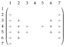
where the left triangle of + signs corresponds to the first double summation and the right triangle corresponds to the second double summation. Since we are trying to compute HT(B_7,4), we will take only the hitting times marked with + in the block B^*₁₁ = B₁₁, i.e.:

Also, proposition 2 states that all non-zero elements of $B_{22}$ are equal to $2(n-1)$, and since there are $\left({\displaystyle \genfrac{}{}{0pt}{}{n-d}{2}}\right)$ pairs of pendant vertices, each of which contributes $2(n-1)$, the total contribution to the $HT$ index taken from $B_{22}$ equals

$$S_2=\left({\displaystyle \genfrac{}{}{0pt}{}{n-d}{2}}\right)2(n-1)=(n-d)(n-d-1)(n-1)$$

(7)

The next proposition deals with the expected hitting times between the pendant vertices and the vertices in the linear part of the broom, in other words, it looks at the contribution to $HT\left(B_{n,d}\right)$ given by the blocks $B_{12}$ and $B_{21}$.

We will look first at the simplest case, which occurs when there are only two pendant vertices, $n-1$ and n, or in other words, we will look at $B_{n,n-2}$. For this case we obtain the following result:

Proposition 3.

In the $B_{n,n-2}$ broom, $n\ge 5$, the following equations hold

$$D(1,n-1)=D(1,n)=E_n{T}_1=n^2-2n-2$$

$$D(i,n-1)=D(i,n)=E_i{T}_n=n^2-4n-i^2+2i+5,$$

(8)

for $2\le i\le n-2$.

Proof. For any $1\le i\le n-2$ we have

$$E_i{T}_n=E_i{T}_{n-2}+E_{n-2}{T}_n=(E_1{T}_{n-2}-E_1{T}_i)+E_{n-2}{T}_n$$

$$={(n-3)}^2-{(i-1)}^2+2n-3=n^2-4n-i^2+2i+5.$$

On the other hand

$$E_n{T}_i=E_n{T}_{n-2}+E_{n-2}{T}_i=1+E_{n-2}{T}_i$$

$$=1+2(n-1)(n-2-i)-[{(n-3)}^2-{(i-1)}^2],$$

where we have used (2) in the last equality. Simplifying we get

$$E_n{T}_i=n^2-2ni+i^2-3.$$

Now let us look at the difference

$$\Delta (i,n)=E_i{T}_n-E_n{T}_i=-4n-2i^2+2ni+2i+8.$$

We have that

$$\Delta (1,n)=-2n+8<0,$$

as long as $n>4$. In other words, $E_1{T}_n<E_n{T}_1$ for $n>4$, proving the first claim of the theorem, that $D(1,n)=E_n{T}_1$. Also,

$$\Delta (2,n)=4,$$

so $E_2{T}_n>E_n{T}_2,$ for all n where the graph is a broom, i.e, $n\ge 5$. And for all other $i\ge 3$ we can show that

$$\Delta (i,n)>0,$$

which is equivalent to showing

$$n(2i-4)>2i^2-2i-8,$$

or

$$n>i+1-{\displaystyle \frac{2}{i-2}},$$

which is true because the only permissible i’s satisfy $i\le n-2$. •

With propositions 2 and 3 we get the contributions of the blocks $B_{21}$ and $B_{22}$:

$$S_3=2(n^2-2n-2)+2\sum _{i=2}^{n-2}(n^2-4n-i^2+2i+5).$$

(9)

Now we are ready to get the first main result.

Proposition 4.

For $n\ge 5$ we have

$$HT\left(B_{n,n-2}\right)=$$

$$\sum _{k=1}^{\lfloor {\displaystyle \frac{n}{2}}\rfloor }\sum _{m=k+1}^{min\{n-k+1,n-2\}}(2n-m-k)(m-k)+\sum _{k=\lfloor {\displaystyle \frac{n}{2}}\rfloor +2}^{n-2}\sum _{m=n-k+2}^{k-1}(m+k-2)(k-m)$$

(10)

$$+{\displaystyle \frac{4}{3}}{n}^3-7n^2+{\displaystyle \frac{65}{3}}n-32.$$

(11)

When $n=5$ or $n=6$, the second double summation is to be taken as 0.

Proof.

The contribution of $B_{11}$ is given by the same values as those of $B_{11}^{*}$, which are found by eliminating from the matrix $E^{*}$ the last two rows and columns, that is, eliminating from the summations in (3) both n and $n-1$ as potential targets or starting points, and that is achieved by tweaking a little the indices of both double summations, as shown in (10). The polynomial in (11) corresponds to the sum of the other contributions $S_2=2(n-1)$ (when $k=2$) and $S_3=2(n^2-2n-2)+2{\sum }_{i=2}^{n-2}(n^2-4n-i^2+2i+5).$•

For example, $HT\left(B_{7,5}\right)=162+234=396$. Here the term 162 corresponds to the double summations in (10), while the term 234 corresponds to the value of the cubic polynomial (11).

As another example, for $n=5$ our formula in proposition 4 yields $HT\left(B_{5,3}\right)=92$, and we notice that $B_{5,3}$ can be thought of as the bi-star $B(3,2)$ for which the formula on p. 13 of [5] (beware: this is the correct formula, not the one given in the statement of their theorem 3) also gives the value $HT\left(B\right(3,2\left)\right)=92$.

After dealing with the extreme case of a broom graph which has the longest path, $P_{n-2}$, and the smallest possible number of pendant vertices, now we want to invert the situation and look at the broom graph with the shortest possible path, which would be $P_3$ (because the choices of $P_1$ and $P_2$ yield star graphs, whose $HT$ index is well known). So we will look first at the broom graph $B_{n,3}$, with $n\ge 6$ (smaller values of n give us graphs with known values of the $HT$ index).

From the matrix viewpoint, the block $B_{11}$ is the smallest of the four blocks on the matrix E, with size $3\times 3$, and if we look at (3) (or at the example above of the matrix with the + signs), we notice that there are only three terms of the first double summation that are inside that small block, namely

$$D(1,2)=E_2{T}_1=2n-3,D(1,3)=E_3{T}_1=4n-8,D(2,3)=E_3{T}_2=2n-5,$$

for a grand total contribution of

$$S_1=8n-16.$$

(12)

The block $S_{22}$ is the largest, of size $(n-3)\times (n-3)$, and its contribution is given by (7) as

$$S_2=(n-1)(n-3)(n-4).$$

(13)

For the contributions of the blocks $B_{12}$ and $B_{21}$, we will look at the general case of the broom graph $B_{n,n-k}$ with k pendant vertices and a path $P_{n-k}$. We will use the vertex n as a generic pendant vertex, and get the following generalization of proposition 3:

Proposition 5.

For $1\le i\le n-k$ in $B_{n,n-k}$ we have

$$E_i{T}_n=n^2-2nk+k^2+2k-i^2+2i-3,$$

(14)

and

$$E_n{T}_i=n^2-2ni+i^2-k^2+1.$$

(15)

Proof. Using (6), we get that for $1\le i\le n-k$

$$E_i{T}_n=E_i{T}_{n-k}+E_{n-k}{T}_n=(E_1{T}_{n-k}-E_1{T}_i)+2n-3$$

$$={(n-k-1)}^2-{(i-1)}^2+2n-3.$$

On the other hand, using (2) we get

$$E_n{T}_i=E_n{T}_{n-k}+E_{n-k}{T}_i$$

$$=1+2(n-1)(n-k-i)-({(n-k-1)}^2-{(i-1)}^2.$$

Expanding and regrouping terms finishes the proof. •

Still working with $B_{n,n-k}$ with k pendant vertices, let us take $n=k+3$, i.e., the case $B_{n,3}$. There are three hitting times of interest, that we compute using (14) and (15):

$$E_n{T}_3={(k+3)}^2-2(k+3)3+9-k^2+1=1,$$

$$E_n{T}_2={(k+3)}^2-2(k+3)2+4-k^2+1=2k+2,$$

$$E_n{T}_1={(k+3)}^2-2(k+3)+1-k^2+1=4k+5.$$

Similarly, going in the other direction

$$E_1{T}_n=2k+7,$$

$$E_2{T}_n=2k+6,$$

$$E_3{T}_n=2k+3.$$

It is clear then that (see Table 1, where we take the maximum value of each row)

$$D(1,n)=4k+5D(2,n)=2k+6D(3,n)=2k+3,$$

and since there are k choices for the pendant vertex, the total contribution of the blocks $B_{21}$ and $B_{12}$ is

$$S_3=k(8k+14)=(n-3)(8n-10).$$

(16)

Finally, we arrive to our second main result:

Proposition 6.

For $n\ge 6$ we have

$$HT\left(B_{n,3}\right)=n^3-7n+2.$$

Proof. It suffices to add $S_1$, $S_2$ and $S_3$ found in (12), (13) and (16), respectively. •

Thus, for example, $HT\left(B_{6,3}\right)=176$ and $HT\left(B_{7,3}\right)=296.$

Now we will look at the broom $B_{n,4}$, with $n\ge 7$ (smaller values of n yield graphs whose $HT$ index is already known). In order to find $HT\left(B_{n,4}\right)$ we notice that the contributions of the blocks $B_{11}$ and $B_{22}$ are clear. The main problem is to find the contributions of the blocks $B_{12}$ and $B_{21}$. Now we will look at $B_{n,4}$ using some recursive formulas. Let us rewrite the parameters as: k pendant vertices and s vertices in the linear part, so that $n=s+k$. Using (14) we get, for $1\le i\le s$:

$$E_i{T}_n={(k+s)}^2-2(k+s)s+k^2+2k-i^2+2i-3$$

$$=s^2+2k-i^2+2i-3.$$

(17)

Now let us increase by one the length of the linear part, keeping the same k pendant vertices, so that $n=k+s+1$ and let us compute the hitting times on the new graph (denote them by $T_n^{\prime }$) of the pendant vertices (again, n is just a representative of any pendant vertex) starting from somewhere in the linear path, i.e., $1\le i\le s+1$. Using (14) we obtain

$$E_i{T}_n^{\prime }={(k+s+1)}^2-2(k+s+1)k+k^2+2k-i^2+2i-3$$

$$=s^2+2k-i^2+2i-3+(2s+1)=E_i{T}_n+(2s+1).$$

(18)

In other words, the new hitting times can be obtained, whenever $1\le i\le s$, as the old hitting times plus the constant $2s+1$. In addition, there is a new hitting time, when $i=s+1$, whose value is

$$E_{s+1}{T}_n^{\prime }={(s+1)}^2+2k-{(s+1)}^2+2(s+1)-3=2k+2s-1.$$

(19)

Going in the opposite direction, it should be clear that $E_n{T}_i^{\prime }=E_n{T}_{i-1}$, for $2\le i\le s+1$, and the only new hitting time is $E_n{T}_1^{\prime }=E_n{T}_1+2n-3$, on account of the time needed for a leaf to be reached from its neighbor. To clarify these ideas, we present a table for the hitting times needed in $B_{n,3}$ and another table showing how the relevant hitting times for $B_{n+1,4}$ are generated from the previous table. Indeed, the rightmost column of Table 3 is generated adding $2s+1=7$ (here $s=3$) to the corresponding column of Table 1, except for the last value, when $i=4$, generated according to (19). Also, the column for the values of $E_n{T}_i$ in Table 3 is obtained by pushing down the corresponding column of Table 1 and when $i=1$, by adding to $4k+5$ the expected time to hit a leaf from a neighbor, which is $2n-3=2k+5$

Table 2. Hitting times for $B_{n,4}$.

i	${\mathit{E}}_{\mathit{n}}{\mathit{T}}_{\mathit{i}}$	${\mathit{E}}_{\mathit{i}}{\mathit{T}}_{\mathit{n}}$
1	$6k+10$	$2k+14$
2	$4k+5$	$2k+13$
3	$2k+2$	$2k+10$
4	1	$2k+5$

Table 2. Hitting times for $B_{n,4}$.

i	${\mathit{E}}_{\mathit{n}}{\mathit{T}}_{\mathit{i}}$	${\mathit{E}}_{\mathit{i}}{\mathit{T}}_{\mathit{n}}$
1	$6k+10$	$2k+14$
2	$4k+5$	$2k+13$
3	$2k+2$	$2k+10$
4	1	$2k+5$

Table 3. Hitting times for $B_{n,5}$.

i	${\mathit{E}}_{\mathit{n}}{\mathit{T}}_{\mathit{i}}$	${\mathit{E}}_{\mathit{i}}{\mathit{T}}_{\mathit{n}}$
1	$8k+17$	$2k+23$
2	$6k+10$	$2k+22$
3	$4k+5$	$2k+19$
4	$2k+2$	$2k+14$
5	1	$2k+7$

Table 3. Hitting times for $B_{n,5}$.

i	${\mathit{E}}_{\mathit{n}}{\mathit{T}}_{\mathit{i}}$	${\mathit{E}}_{\mathit{i}}{\mathit{T}}_{\mathit{n}}$
1	$8k+17$	$2k+23$
2	$6k+10$	$2k+22$
3	$4k+5$	$2k+19$
4	$2k+2$	$2k+14$
5	1	$2k+7$

This means that the contribution of the blocks $B_{21}$ and $B_{21}$ is

$$S_3=k[(2k+5)+(2k+10)+(2k+13)+(6k+10)]=k(12k+38)=222\mathrm{if}k=3,$$

and

$$S_3=k[(2k+5)+(2k+10)+(4k+5)+(6k+10)]=k(14k+30)=(n-4)(14n-26)\mathrm{if}k\ge 4.$$

The contribution due to the block $B_{22}$ is simple, given by

$$S_2=(n-4)(n-5)(n-1).$$

As for the contribution of $B_{11}$, we see that we need to compute

$$S_1=E_2{T}_1+E_3{T}_1+E_4{T}_1+E_3{T}_2+E_4{T}_2+E_4{T}_3=20n-50.$$

Finally, adding $S_{1,2}$ and $S_3$ we get the following

Proposition 7.

The following equalities hold:

$$HT\left(B_{7,4}\right)=348.$$

$$HT\left(B_{n,4}\right)=n^3+4n^2-33n+34\mathrm{for}n\ge 8.$$

Thus, for example, $HT\left(B_{8,4}\right)=538$.

3. Final Remarks

As seen in the previous section, our method consists of considering three contributions to the value $HT\left(B_{n,d}\right)$. The first one, $S_1$, is due to the hitting times contained in the block $B_{11}$, and this is found by looking at the hitting times contained in the block $B_{11}^{*}$ of the $E^{*}$ matrix of the n-path $P_n$. The second and simplest, $S_2$, is due to the (identical) times, starting from a pendant vertex, to hit another pendant vertex, and these times are contained in the block $B_{22}$. Finally, the toughest analysis is that of deciding which times we select from the blocks $B_{12}$ and $B_{21}$ in order to get the last contribution $S_3$.

If, for example, we wanted to find a formula for $HT\left(B_{n,n-3}\right)$, i. e.: the case with only three pendant vertices, we would need to truncate the matrix $E^{*}$ eliminating the last three rows and columns from our analysis, in order to get $S_1$. Also, we would need to apply theorem 5 in order to get $S_3$. As usual, the computation of $S_2$ would be simple.

In the other direction, if we wanted to compute $HT\left(B_{n,5}\right)$, the recursive argument we used to go from $B_{n,3}$ to $B_{n,4}$ would be applicable, and would simplify finding the contribution $S_3$. Indeed, the table of relevant hitting times to be compared would be the following, found by copying the values, of the previous table, of the column for $E_n{T}_i$ from the bottom up, and including the new entry $8k+17$ (adding to the previous value $6k+10$ one hitting time of a leaf from a neighbor), and also by copying the column for $E_i{T}_n$ from the top down, and adding $2s+1=9$ to all entries in this column, and introducing the new value $2k+7$ generated using (19).

We will leave the details of these calculations to the interested reader.

References

- Buckley, F.; Harary, F. Distance in graphs; Addison-Wesley Publishing Company: Redwood City, CA, USA, 1990. [Google Scholar]
- Chandra, A. K.; Raghavan, P.; Ruzzo, W. L.; Smolensky, R.; Tiwari, P. The electrical resistance of a graph captures its commute and cover times. Comput. Complexity 1996, 6, 312–340. [Google Scholar] [CrossRef]
- Grinstead, M.; Snell, J. L. Introduction to Probability, 2nd. ed.; American Mathematical Society: Providence, RI, 1997. [Google Scholar]
- Doyle, P. G.; Snell, J. L. Random walks and electrical networks; The Mathematical Association of America: Washington, D.C., 1984. [Google Scholar]
- He, M.; Mao, Y.; Furtula, B.; Zhang, X. Hitting time index of trees. J. Math. Chem. 2026, 64. [Google Scholar] [CrossRef]
- Palacios, J. L. A new probabilistic molecular index. MATCH Commun. Math. Comput. Chem. 2025, 93, 499–507. [Google Scholar] [CrossRef]
- Palacios, J. L.; Santamaría, A. Some new results for the hitting time index. MATCH Commun. Math. Comput. Chem. 2025, 94, 427–445. [Google Scholar] [CrossRef]
- Palacios, J. L.; Santamaría, A. On the hitting time index of graphs. Open J. Appl. Sci. 2025, 4, 2464–2478. [Google Scholar] [CrossRef]
Disclaimer/Publisher’s Note: The statements, opinions and data contained in all publications are solely those of the individual author(s) and contributor(s) and not of MDPI and/or the editor(s). MDPI and/or the editor(s) disclaim responsibility for any injury to people or property resulting from any ideas, methods, instructions or products referred to in the content. |
© 2026 by the authors. Licensee MDPI, Basel, Switzerland. This article is an open access article distributed under the terms and conditions of the Creative Commons Attribution (CC BY) license (http://creativecommons.org/licenses/by/4.0/).
Copyright: This open access article is published under a Creative Commons CC BY 4.0 license, which permit the free download, distribution, and reuse, provided that the author and preprint are cited in any reuse.