
Submitted:
30 March 2026
Posted:
31 March 2026
You are already at the latest version
Abstract
Small and medium-sized enterprises are prone to errors or evasion in areas such as medical insurance reimbursement, pension contributions, and unemployment insurance, which not only harm workers' rights but also impact the sustainability of federal and state public funds. Therefore, an explainable intelligent tax compliance screening system is urgently needed. This paper uses multi-task learning as the backbone, while modeling the shared risk representations of sub-tasks such as wages, pensions, unemployment insurance, and medical insurance contributions. Subsequently, our model combines multi-task learning with time-series anomaly detection to capture overlooked scenarios and structural avoidance in long-term trends. On heterogeneous time-series graphs, SHapley Additive exPlanations (SHAP) contributions are propagated and decomposed according to 'feature-module-time-task,' and combined with gated dependencies and consistency constraints to generate auditable risk paths, achieving an upgrade from anomaly scoring to evidence-chain visualization. Experiments show that this method improves both identification performance and interpretable localization efficiency.
Keywords:
CCS concepts
; computing methodologies
; machine learning
; machine learning approaches
; neural networks
; payroll tax compliance
; anomaly attribution
; SHAP explanations
; multi-task learning
; risk path generation
1. Introduction
Payroll tax compliance screening sits at the intersection of labor protection and fiscal sustainability. For many small and medium-sized businesses, payroll reporting is not a single ledger problem but a coupled system. Gross wages, overtime and bonuses, withholding, employer-side contributions, benefit plan payments, and health insurance–related records must align across multiple reporting channels and over time 1. When misreporting, underpayment, or strategic avoidance occurs, the downstream impact is twofold. Workers may lose eligibility or continuity of benefits, and federal trust funds face cumulative leakage that undermines long-run solvency.
Traditional compliance workflows often rely on rule engines and threshold checks including abnormal wage growth, contribution ratios outside expected bounds, sudden changes in filing frequency, or mismatches between headcount and total payroll. While these heuristics are easy to explain, they are brittle against evolving evasion strategies and cross-form inconsistencies that only become apparent when multiple data streams are integrated 2. Conversely, end-to-end machine learning models can improve detection accuracy but frequently fail to translate into actionable audit decisions because their outputs are not naturally aligned with how auditors gather evidence.
A major difficulty in this domain lies in heterogeneous data and semantic misalignment across sources. Payroll records, benefits contributions, and health insurance–related information are generated by different operational processes and may use different identifiers, timing conventions, and aggregation levels. Distributions also vary by industry, geography, firm size, and employment composition, which can cause naïve models to confuse structural differences with noncompliance 3. Moreover, reasonable explanations for changes seasonality, workforce turnover, shifts from full-time to part-time, changes in benefit enrollment can mimic the statistical footprint of evasion. The model must therefore reconcile cross-domain signals while remaining robust to legitimate heterogeneity, and it must do in a way that supports human validation.
Another challenge is the time gap of compliance risk. Much lapsing behavior isn’t the single big shock so much as small tweaks that compound: slowly pushing down the reported wage bases, nudging compensation into more opaque buckets, delaying or reducing contributions over a number of quarters. Meanwhile policy and macro economics are introducing concept drift, changing what the “normal” levels and correlations look like. Hard thresholds, one-off regimes of training fall flat 4.
To meet these needs, we propose SHAP-Guided Risk Path Generation for IRS auditors, a framework that treats interpretability as a first-class objective rather than a post-hoc add-on. The method begins with a multi-task architecture that learns a shared latent representation spanning payroll, benefits, and healthcare-related compliance tasks, while preserving task-specific decision boundaries through dedicated heads. It then applies temporal anomaly detection to identify both abrupt irregularities and slow deviations in longitudinal patterns. Crucially, instead of stopping at feature attribution, we use SHAP-driven contributions as inputs to a path-generation procedure that assembles a coherent evidence chain an ordered sequence of time-stamped, module linked drivers.
2. Related Work
Islam 5 uses long-panel data to discuss how AI-enhanced tax risk scoring can be used to more systematically segment taxpayers, improve audit coverage, and increase resource allocation efficiency. Hu 6 reported a comparison with baselines such as random forests and unidirectional LSTM, and used Attention visualization and SHAP values to interpret the key drivers of the model in time series, thus presenting both ‘when an anomaly occurs and why it occurs.’
Henderson et al. 7 describe setting and study the corresponding mechanisms for optimize-and-estimate structured bandits, and they also investigate how their method performs under real-world constraints like delayed feedback, distribution drift, and other practical limitations provided in the context of real tax data collaborations, showing that they can improve the overall estimation bias while maintaining high detection gains. Zhang 8 proposes an adaptive and interpretable AI framework for tax scenarios targeting small and medium-sized enterprises, emphasizing the upgrade of tax risk scoring from merely a passive audit trigger to an actionable risk mitigation closed loop. By leveraging interpretability techniques such as SHAP to identify major risk sources and feeding the explanation results back into the enterprise’s compliance management processes, proactive governance can be achieved. Recent advances in large language models have also shown promise in financial text analysis tasks, with efficient fine-tuning methods enabling domain-specific adaptation [9].
From a policy evaluation perspective, Jess Grana et al. 10 examine tax authority audits as the research subject, quantifying the ‘specific indirect effects’ of audits on taxpayers’ subsequent reporting behavior beyond direct recovery, and point out that in audit resource allocation, direct effects, costs, and long-term behavioral responses should all be considered to achieve a more optimal enforcement input-output. At the engineering methodology level, Anas AlSobeh et al. 11 propose a hybrid framework for proactive tax fraud detection using interpretable AI, employing GBDT and attention-based deep networks for parallel modeling and prediction fusion, while combining SHAP and attention heatmaps to enhance transparency for auditors.
Harger and Nickel 12 emphasized that in an environment of time-consuming APAs, increased cross-border uncertainty, and enhanced U.S. enforcement resources and audit intensity, tax insurance can transfer uncertain tax liabilities in a way that aligns more closely with commercial timelines, cover dispute defense costs, and replace or reduce escrows in transaction negotiations, thereby improving the certainty of tax risk pricing and capital allocation. Olumoh and Mubaraq 13 noted that audit management and tax control mechanisms have a significant positive impact on SIRS performance; based on this, they recommend strengthening strategic audit plans, case tracking, and risk-based independent reviews, increasing supplemental taxes, improving documentation and structured compliance processes, and enhancing risk governance capabilities through regular assessments and benchmarking against international standards.
Chen et al. 14 constructed a normative analytical model combining cash flow uncertainty and tax uncertainty, treating advance tax rulings as a fee-based tax certainty tool. They systematically described how tax system elements and loss offset mechanisms jointly influence a firm’s optimal investment intensity in high-risk projects, and further derived, from the tax authority’s perspective, the ATR charging range that balances the welfare of both parties.
3. Methodologies
3.1. Multi-Task Dual-Channel Temporal Risk Scoring
Above all, we denote a taxpayer by , time by , and module by for Payroll, Benefits, and Healthcare. The raw feature vector for module at time is , and the missingness mask is . We concatenate masked values and the mask to form the effective input so the model can learn patterns, which are common in compliance data and should not be treated as random noise by Equation (1).
where denotes element-wise multiplication, ensuring unobserved values do not leak arbitrary numerical placeholders into the network. The concatenation operator appends the binary mask so downstream layers can condition at each feature position. Because modules differ in scale and semantics, we embed each module into a common latent space before cross-module fusion. This projection also reduces heteroskedasticity across modules and creates a unified interface for later temporal modeling. We use a module-specific nonlinear encoder to produce a fixed-width representation , enabling apples-to-apples fusion between Payroll, Benefits, and Healthcare signals by Equation (2).
where and are learnable matrices tailored to module , while is a pointwise nonlinearity. The hidden width is shared across modules so that later attention or gating operations can compare and combine module embeddings.
We explicitly define three supervised tasks and one self-supervised temporal task: T1 predicts a risk probability for proxy label using binary cross-entropy ; T2 predicts a severity score for proxy severity using Huber loss ; T3 predicts a consistency-anomaly probability for sublabel derived from cross-field residual exceedance using .
To jointly learn payroll risk factors across multiple compliance tasks, we adopt a shared Mixture-of-Experts (MoE) trunk with task-adaptive routing. The core rationale is that some latent risk mechanisms are shared, while different tasks emphasize different slices of the signal. MoE decomposes representation learning into multiple experts and uses a gating network per task to select and weight these experts, both shared learning and task-specific flexibility as Equation (3).
Each expert can be instantiated as a cross-module attention block or a multilayer fusion network. The number of experts controls capacity and the diversity of learned risk mechanisms. Practically, experts allow the model to separate patterns, which improves both detection accuracy and downstream interpretability. We compute task-specific gating weights from the concatenated module embeddings. This explicit routing also provides an internal dependency signal that we later reuse when constructing gated edges for risk-path generation. The softmax normalization ensures the routing weights are nonnegative and sum to Equation (4), which is valuable for stability and for interpreting which experts dominate each task at each time.
In above gating equation, is a task-specific projection, and the concatenation aggregates the three module embeddings into a single routing context. The index denotes compliance tasks; for example, can represent noncompliance classification, underpayment magnitude regression, cross-form inconsistency detection, etc. Because routing is computed at each , the model can adapt when a firm’s behavior changes over time, which is essential for detecting gradual drifts rather than only abrupt shocks.
The shared task representation is then the convex combination of expert outputs. Equation (5) integrates payroll, benefits, and healthcare risk factors into a single task-conditioned state, while maintaining separability across tasks. This representation is the input to the temporal anomaly detector.
where is the expert output width, and is the -th component of the gating vector. The convex structure yields numerical stability and an implicit regularization effect that reduces overfitting on noisy compliance signals. Conceptually, represents the model believes matters right now for task after looking jointly at payroll, benefits, and healthcare inputs.
Subsequently, we score time-varying anomalies using a dual-channel temporal architecture by Equation (6). A Transformer channel for long-range dependencies and an LSTM channel for local drift and seasonal residuals. This design mirrors real-world compliance dynamics, where evasion can be gradual or sudden. Running both channels in parallel and fusing them improves sensitivity across different anomaly regimes.
In the Transformer channel, is a positional encoding that injects time order information, and selects the -th output token. In the LSTM channel, the recurrent state naturally models local patterns such as month-to-month payroll changes or contribution timing effects. We use task-specific temporal models and so that each compliance target can emphasize different temporal structures. We fuse both temporal embeddings to produce the final task risk score . For regression tasks we replace it with an appropriate output layer. This fused score is the risk score that triggers the subsequent interpretability and risk-path stages by Equation (7).
The vector and bias are task-specific parameters; the concatenation allows each task to learn how much to trust long-range versus local evidence. This fusion step is intentionally simple because we want interpretability to remain tractable when later attributing risk to upstream features. Overly complex fusion can make SHAP-based decompositions less stable in high-dimensional temporal settings.
We generate interpretable risk paths on a directed acyclic graph (DAG) whose nodes are module–time pairs . We include only time-forward edges to preserve causality and optionally same-time cross-module edges when a learned dependency is present. Each node receives a score computed by aggregating SHAP attributions within module.
Finally, to stabilize audit triggers and reduce oscillatory alerts, we add a bidirectional consistency regularization between the Transformer-only posterior and the LSTM-only posterior. This directly implements the abstract’s claim of consistency constraints in the temporal detector. In practice, it discourages cases where one channel signals high risk while the other signals low risk without strong evidence by Equations (8) and (9).
where and produce channel-specific posteriors, and is the Kullback–Leibler divergence. The symmetric KL form penalizes disagreement in both directions, improving calibration and temporal stability. KL divergence is only defined between valid probability distributions. Therefore, for each supervised task we convert both channels’ outputs into distributions before applying KL. For binary tasks (T1, T3), each channel produces a logit , and we form Bernoulli parameters . We then compute to enforce consistency between Transformer and LSTM channels.
3.2. SHAP-Guided Risk Path Generation on a Heterogeneous Temporal Graph
Furthermore, we begin by defining SHAP attributions at the level of task and evaluation time . Let denote the trained predictor producing from the full set of input features within the window . Expand the full feature set into a flattened index that includes module, time, and atomic feature coordinates. SHAP defines the contribution of each feature as a Shapley value from cooperative game theory, guaranteeing additivity and a fair allocation of the prediction difference from a baseline as Equation (10).
In above expression, ranges over all subsets of features excluding , and denotes the model prediction when only features in are present. The factorial weighting term is the canonical Shapley coefficient that averages marginal contributions over all feature orderings. We use SHAP because its additivity enables accounting consistency, meaning auditors can reconcile a path-level explanation back to the model score without hidden residuals.
We compute (a) cross-field consistency residuals defined by domain-agnostic constraints , and (b) temporal jump scores normalized within peer groups to reduce scale effects. A sample is labeled positive if any year violates a high-confidence threshold.To align explanations with audit practice, we do not keep SHAP at the atomic feature level. Instead, we explicitly index each feature as a triple , where is the module, is the time index, and is the atomic feature within module . This yields a granular attribution tensor , which we then aggregate to produce interpretable units as Equation (11).
where represents which module at which time drove risk, measures which time window is most suspicious, and denotes which compliance module is the dominant source.
However, even module–time attributions can remain fragmented, producing many small peaks rather than a coherent narrative. To assemble a risk path, we build a heterogeneous temporal graph for each taxpayer , where nodes represent module–time pairs and edges encode two kinds of structure: temporal continuity within the same module and contemporaneous coupling across modules. This graph formalizes the risk transmission intuition used by auditors when they trace inconsistencies from payroll to benefits to healthcare obligations by Equation (12).
Nodes correspond to the audit-relevant unit module at time . The edge set includes intra-module temporal edges and cross-module edges for . Temporal edges capture drift and persistence, while cross-module edges capture structural mismatch mechanisms.
We explicitly partition variables into a rule only set and a model feature set . We enforce: , and any deterministic transform of rule variables including threshold indicators, binned versions, rule residuals , jump scores , and any features directly used to compute the proxy label is excluded from . To ensure paths reflect taxpayer-specific dynamics rather than global averages, we parameterize edge weights with gated dependencies by Equation (13).
The quantity is a representation-level change magnitude that highlights potential structural breaks or sudden shifts in a module’s latent state. The gating entropy measures how concentrated the task routing is over experts, lower entropy means a clearer underlying mechanism, which we treat as more reliable for constructing paths. For module with raw features, let be the raw input at time , and let be a binary availability mask.
4. Experiments
4.1. Experimental Setup
The experiment selected the Individual Public-Use Microdata File (PUF) for Tax Years 2012–2015 released by the IRS Statistics of Income (SOI), which is derived from a sample of U.S. federal individual income tax returns and is provided in the form of publicly available microdata files for academic research and policy analysis. To protect taxpayer privacy, the PUF undergoes statistical alteration before release, so while retaining the structure of actual filing behavior and the relationships between variables. Empirical evaluation in this paper uses the IRS SOI Individual Public-Use Microdata File (PUF) (tax years 2012–2015). To make the narrative and experiments consistent, we treat “Payroll/Benefits/Healthcare” as proxy compliance modules constructed from semantically related PUF fields rather than claiming access to employer payroll tax forms.
Since the PUF does not contain audit conclusions, we construct risk proxy labels using cross-field consistency constraints and abnormal jump rules, and incorporate a self-supervised temporal anomaly task to enhance sensitivity to gradual drift. After deduplicating the data by taxpayer entity, we split it into training, validation, and test sets, and use rolling evaluation to assess cross-year generalization. Comparisons include traditional risk models, single-channel LSTM and Transformer, as well as ablation of key components. Metrics report identification performance, alarm stability, and the sparsity and verifiability of risk pathways.
4.2. Experimental Analysis
Figure 1 shows that the proposed SHAP-Guided Risk Path model achieves the most favorable trade-off between true positive rate and false positive rate, with its curve closest to the top-left corner and an AUROC of 0.997, indicating near-perfect discrimination across thresholds. We compute feature attributions using DeepSHAP (SHAP DeepExplainer) for neural networks. The baseline distribution is constructed by sampling 256 sequences from the training set using stratification on the proxy label to ensure coverage of both typical and atypical patterns; we repeat this sampling 5 times and average attributions across runs to improve stability.
The ablation without the gated graph structure drops to 0.984, still strong but clearly worse, suggesting that the gated dependency/structured component contributes meaningfully to separability. The Single-Channel LSTM and XGBoost baselines perform similarly (0.956 and 0.955), with curves bending downward earlier in the low-FPR region, implying reduced sensitivity when auditors require very low false-alarm rates. Logistic Regression lags behind (0.877) and remains much closer to the random diagonal, reflecting the limitations of linear decision boundaries for capturing nonlinear, cross-module, and temporally evolving compliance risk patterns.
Figure 2 compares Precision@k under different audit budget levels and shows that the proposed SHAP-Guided Risk Path method consistently achieves the highest top-k hit rate across all budgets, especially in the low-budget regime where audit capacity is most constrained. As the review budget increases from very small fractions to several percent of taxpayers, Precision@k decreases for all methods, which is expected because the model must include increasingly lower-ranked cases; however, the proposed method degrades more slowly, indicating better ranking quality and stronger concentration of true high-risk cases at the top of the list.
Table 1 evaluates how often model alerts “jump” using Top-k Jaccard similarity and temporal score smoothness. The proposed SHAP-Guided Risk Path achieves the highest Jaccard values across Top-0.5%, Top-1%, and Top-2% and the smallest , indicating the most stable audit shortlist and the smoothest risk trajectories. Removing key components, especially the consistency loss reduces Jaccard and increases score volatility, showing these modules are critical for stable triage. All reported metrics are measured under the anti-leak protocol described above. Under this controlled setting, the proposed method achieves AUROC = 0.997, outperforming ablations and baselines including 0.984 without the gated graph component; 0.956 for a single LSTM; 0.955 for XGBoost; and 0.877 for logistic regression.
5. Conclusions
In conclusion, we proposed a SHAP-Guided Risk Path framework for IRS-oriented payroll tax screening that combines multi-task shared representations with a Transformer+LSTM dual-channel detector to produce robust risk ranking, and then organizes SHAP attributions on a heterogeneous temporal graph into auditable evidence-chain paths. Experiments show consistent gains in AUROC, AUPRC, Top-k hit rate, and alert stability over strong baselines and ablations. Looking ahead, we will incorporate real audit feedback and stronger causal constraints, extend to firm-level multi-form datasets.
References
- Colak, M., & Sarioglu, M. (2025). The Effect of Corporate Governance on the Quality of Integrated Reporting and ESG Risk Ratings. Sustainability, 17(11), 4868. [CrossRef]
- Lane, C. (2025). Let’s Jettison Some Executive Perks: Exploring the SEC and IRS Approaches to Personal Use of Corporate Aircraft. J. Air L. & Com., 90, 265.
- Huang, F., Wang, T., & Yen, J. C. (2024). Opportunities or challenges? Audit risk and blockchain disclosures in 10-K filings. Auditing: A Journal of Practice & Theory, 43(2), 131-158.
- Olvera, P. D. N. (2025). Artificial Intelligence and Algorithms in Tax Auditing by the Tax Administration Service in Mexico: Analysis of Potential Biases. International Journal for Public Policy, Law and Development, 2(3), 18-33.
- Islam, M. R. (2025). AI-Augmented Tax Risk Scoring for Small and Medium Enterprises: A Panel Data Study. ASRC Procedia: Global Perspectives in Science and Scholarship, 1(01), 501-531. [CrossRef]
- Hu, Q. (2025, August). Research on Dynamic Identification and Prediction Model of Tax Fraud Based on Deep Learning. In 2025 2nd International Conference on Intelligent Algorithms for Computational Intelligence Systems (IACIS) (pp. 1-6). IEEE.
- Henderson, P., Chugg, B., Anderson, B., Altenburger, K., Turk, A., Guyton, J., ... & Ho, D. E. (2023, June). Integrating reward maximization and population estimation: Sequential decision-making for Internal Revenue Service audit selection. In Proceedings of the AAAI Conference on Artificial Intelligence (Vol. 37, No. 4, pp. 5087-5095). [CrossRef]
- Zhang, T. (2025, October). From Black Box to Actionable Insights: An Adaptive Explainable AI Framework for Proactive Tax Risk Mitigation in Small and Medium Enterprises. In Proceedings of the 2025 2nd International Conference on Digital Economy and Computer Science (pp. 193-199).
- Lian, Z. (2025, October). Financial Text Classification Based On rLoRA Finetuning On Qwen3-8B model. In Proceedings of the 2025 2nd International Conference on Digital Economy and Computer Science (pp. 225-230).
- Grana, J., Lindsay, I., Lykke, L., McGill, M., McGlothlin, A., Nicholl, L., & Plumley, A. (2025). The specific indirect effect of IRS audits. International Tax and Public Finance, 32(4), 995-1029. [CrossRef]
- AlSobeh, A., Abo El Rob, M. F., Rouibah, K., & Shatnawi, A. (2025). Proactive detection of tax fraud using explainable AI techniques: A hybrid approach. Issues in Information Systems, 26(3).
- Harger, J., & Nickel, M. (2025). How Tax Insurance Can Be a Valuable Tool for Managing Transfer Pricing Risk in 2025 and Beyond. Tax Executive, 77, 62.
- Olumoh, Y. A., & Mubaraq, S. (2025). The Tax Audit Management, Tax Control Mechanisms, and the Performance of State Internal Revenue Services in South-West, Nigeria. FUDMA Journal of Accounting and Finance Research [FUJAFR], 3(3), 1-20. [CrossRef]
- Chen, A., Hieber, P., & Sureth-Sloane, C. (2025). How much to pay for tax certainty? The role of advance tax rulings for risky investment under loss offset and tax uncertainty. International Tax and Public Finance, 1-37. [CrossRef]
Figure 1.
ROC Comparison of Tax Compliance Risk Screening Models.
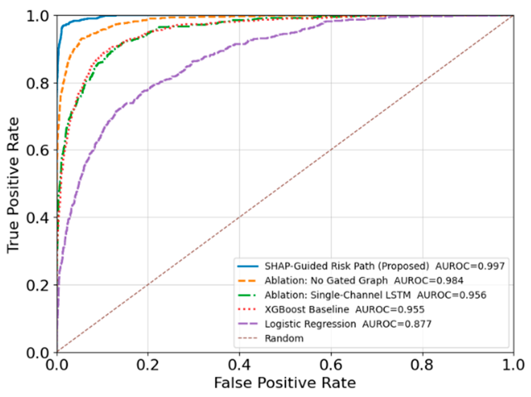
Figure 2.
Top-k Hit Rate (Precision@k) With Audit Budget.
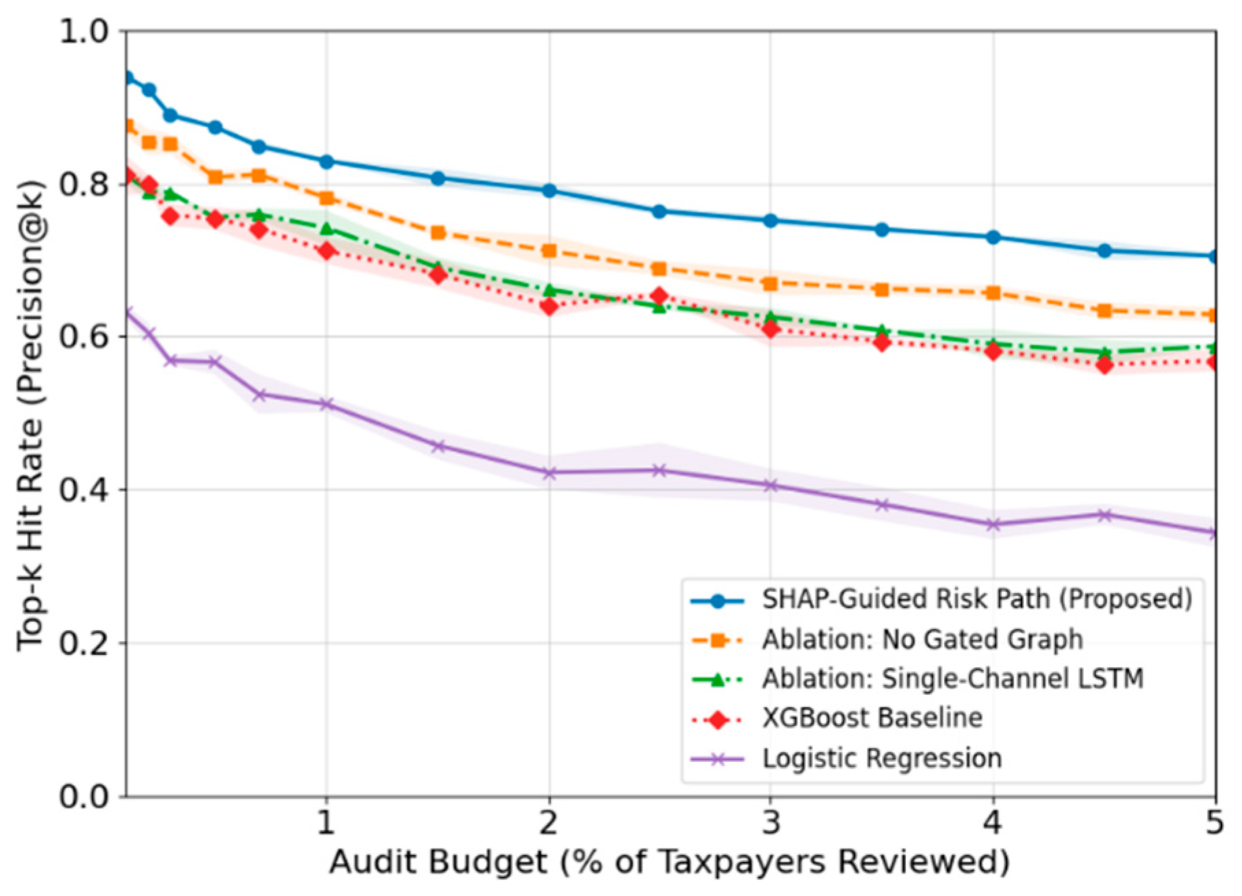

Table 1.
Alert Stability Evaluation via Top-k Jaccard Similarity and Temporal Smoothness.
| Method | Jaccard Top 0.5% | Jaccard Top 1% | Jaccard Top 2% | Time Smoothness Mean |Δscore| | Time Smoothness Std |Δscore| |
| SHAP-Guided Risk Path Proposed | 0.78 | 0.75 | 0.72 | 0.03 | 0.02 |
| Ablation No Gated Graph | 0.70 | 0.67 | 0.64 | 0.04 | 0.03 |
| Single-Channel LSTM | 0.60 | 0.58 | 0.55 | 0.06 | 0.04 |
| Single-Channel Transformer | 0.61 | 0.59 | 0.56 | 0.06 | 0.04 |
| XGBoost Baseline | 0.58 | 0.56 | 0.53 | 0.07 | 0.04 |
| Random Forest Baseline | 0.55 | 0.53 | 0.50 | 0.07 | 0.05 |
| Logistic Regression | 0.44 | 0.42 | 0.4 | 0.08 | 0.05 |
| MLP Baseline | 0.52 | 0.50 | 0.48 | 0.07 | 0.05 |
| Isolation Forest Unsupervised | 0.47 | 0.45 | 0.43 | 0.09 | 0.06 |
| One-Class SVM Unsupervised | 0.45 | 0.43 | 0.41 | 0.10 | 0.06 |
Disclaimer/Publisher’s Note: The statements, opinions and data contained in all publications are solely those of the individual author(s) and contributor(s) and not of MDPI and/or the editor(s). MDPI and/or the editor(s) disclaim responsibility for any injury to people or property resulting from any ideas, methods, instructions or products referred to in the content. |
© 2026 by the authors. Licensee MDPI, Basel, Switzerland. This article is an open access article distributed under the terms and conditions of the Creative Commons Attribution (CC BY) license (http://creativecommons.org/licenses/by/4.0/).
Copyright: This open access article is published under a Creative Commons CC BY 4.0 license, which permit the free download, distribution, and reuse, provided that the author and preprint are cited in any reuse.


