
Submitted:
26 March 2026
Posted:
30 March 2026
You are already at the latest version
Abstract
We propose a field-transformation-based framework for generating phase-only light-field holograms from a single RGB image. The method establishes an explicit pipeline from monocular scene inference to holographic wavefront synthesis, without requiring multi-view capture or task-specific hologram-network training. First, we construct a layered occlusion RGB-D model from the input image using monocular depth estimation, connectivity-based layer decomposition, and occlusion-aware inpainting, which provides a lightweight 3D prior for sparse-view rendering in the small-parallax regime. Second, we transform the rendered sparse RGB-D light field into a target complex wavefront on the recording plane through local frequency mapping, thereby bridging explicit scene geometry and wave-optical field construction. Third, we optimize the phase-only hologram under multi-planeamplitude constraints using a geometrically consistent initial phase and an error-driven adaptive depth-sampling strategy, which improves convergence stability and reconstruction quality under a limited computational budget. Numerical experiments show that the proposed method achieves better depth continuity, occlusion fidelity, and lower speckle noise than representative layer-based and point-based methods, and improves the average PSNR and SSIM by approximately 3 dB and 0.15, respectively, over Hogel-Free Holography. Optical experiments further confirm the physical feasibility and robustness of the proposed framework.
Keywords:
computer-generated holography
; light-field holography
; phase-only hologram optimization
1. Introduction
Computer-generated holography (CGH) numerically synthesizes the complex wavefront of a 3D scene and reconstructs it using a spatial light modulator (SLM). Building on the early development of computer-generated holograms and subsequent advances in digital holography, CGH has become a key technique for wavefront reconstruction, computational imaging, and 3D holographic display [1,2,3,4,5]. Compared with conventional 3D light-field displays, CGH performs encoding and modulation at the wavefront level, enabling not only multi-view parallax reconstruction but also providing visual cues such as defocus and continuous depth.
Existing CGH methods can be organized from several complementary viewpoints. From the viewpoint of computational strategy, representative approaches include direct or non-iterative methods, iterative optimization methods, camera-in-the-loop schemes, and deep-learning-based generators. Direct formulations have been explored through, for example, non-convex optimization and ray-sampling-plane-based color hologram generation with multi-GPU acceleration [6,7]. Iterative methods span classical Gerchberg–Saxton and error-reduction algorithms as well as more recent random-trajectory and adaptive dynamic feedback strategies [8,9]. Camera-in-the-loop methods further improve practical reconstruction quality by explicitly compensating device nonidealities during optimization [10,11]. Deep learning has also enabled fast hologram synthesis, including ResNet-type approaches, depth-aware hologram networks, customizable 3D hologram generators, and diffraction-model-driven high-resolution designs [12,13,14,15]. These taxonomies are complementary rather than mutually exclusive, because a CGH pipeline may simultaneously adopt a particular scene representation, an optimization strategy, and a hardware compensation scheme.
In 3D holographic reconstruction, the ability to represent scene geometry, occlusion relationships, and depth continuity jointly determines the quality of the reconstructed optical field. Because the present work focuses on how a single RGB image is lifted to a 3D scene prior and then transformed into a target complex wavefront, we discuss related methods mainly from the perspective of scene representation and wavefront construction. From this representation-oriented viewpoint, typical CGH pipelines can be broadly categorized into three classes: multi-layer image-based methods (layered holography) [16], point-based methods (point-source holography) [17,18], and light-field-based methods (light-field holography) [19,20]. Among layered holography, RGB-D image pairs are one of the most commonly used forms of 3D representation. These methods typically discretize the 3D scene along the depth direction into multiple 2D depth layers, and then use propagation models such as angular-spectrum diffraction to propagate each layer and superpose their wavefronts on the hologram plane, thereby obtaining the complex wavefield of the 3D scene. Layered holography can be efficiently implemented in combination with the fast Fourier transform (FFT) [21]. However, the superposition of wavefronts from different depth layers leads to severe phase wrapping, making it difficult for the resulting phase-only hologram to faithfully encode the true depth of the scene. To alleviate this issue, one can adopt a finer-grained 3D representation with more controllable wavefronts, by refining the image-level depth-layer representation into a point-source-level description of the scene.
Point-source holography discretizes the 3D scene into a set of point light sources and obtains the complex wavefield of the scene by linearly superposing the sub-wavefronts of all points on the hologram plane. Compared with layered holography, point-source holography can more accurately describe the complex-amplitude distribution at arbitrary positions in 3D space. The independence among the wavefronts of different point sources helps alleviate phase-unwrapping issues introduced by image-level operations, thereby enabling higher-fidelity 3D reconstruction. However, as the number of point sources increases, both reconstruction noise and computational cost grow rapidly, which severely limits the practicality of point-source holography for complex scenes. In addition, for scenes with complex geometry and occlusion relationships, point-source holography typically require additional occlusion-handling strategies, leading to a trade-off between reconstruction quality and computational cost [22,23].
In contrast to the above two categories, light-field holography represents a distinct CGH paradigm. These methods are grounded in Fourier optical imaging theory and encode multi-view light fields to indirectly represent the geometry and occlusion structure of a 3D scene. Since the light-field model explicitly incorporates multi-view information of the scene, it provides a natural basis for occlusion handling, and thus light-field holography has attracted extensive interest for occlusion modeling. Existing work constructs holographic elements (hogels) to provide natural occlusion effects and a relatively continuous depth perception [24,25]. However, such approaches essentially use holography to implement 3D light-field display, and require computing a large number of non-overlapping hogels from the light-field images. As a result, they inevitably suffer from parallax discontinuities caused by limited angular sampling. Hogel-Free Holography (HFH) [26] removes the dependence on hogels by directly inverting a multi-view RGB-D light field to obtain the target complex wavefront. It then combines angular-spectrum diffraction with multi-plane amplitude constraints to optimize a phase-only hologram within a 3D volume. Leveraging the intrinsic parallax information encoded in the light field, HFH exhibits clear advantages in modeling occlusion relationships and maintaining depth continuity. It can better reconstruct multi-view parallax and mitigate the common issues of depth discretization and unnatural occlusions in layered holography and point-source holography.
However, HFH also has several limitations. First, HFH relies on a high-resolution RGB-D light field as input, and the resolution of each viewpoint image is required to match that of the hologram, which imposes a heavy computational burden on the upstream rendering pipeline. Second, HFH performs iterative optimization in a 3D volume starting from a random initial phase, and its convergence behavior is highly sensitive to the choice of the initial phase. As the number of target amplitude constraint planes increases, the nonconvexity of the optimization problem becomes more severe, making convergence difficult and prone to poor local minima, which in turn limits the stability of HFH in practical applications.
On the other hand, single-view 3D reconstruction has advanced rapidly in recent years, enabling the recovery of scene geometry and limited novel-view information from only one RGB image [27,28,29]. Monocular depth estimation and layered scene representations, such as layered depth images, have been widely used for novel-view synthesis from single-view inputs [30,31]. However, most existing single-view methods are developed for photorealistic view synthesis and are primarily optimized for reprojection fidelity or texture completion, rather than for angular-spectrum consistency, wave-optical propagation, or phase-only hologram encoding [32]. Consequently, it remains insufficiently explored how to couple a monocular 3D prior with light-field-based CGH in a physically consistent and computationally efficient manner.
It is also important to distinguish the present problem from conventional multi-plane or extended-depth-of-field holographic reconstruction strategies. Such methods typically assume that target distributions on multiple axial planes are already available, and the main task is then to optimize a hologram that reproduces those prescribed plane-wise constraints. In contrast, the problem considered here starts from only a single RGB observation and must first construct a physically consistent target wavefront that preserves scene geometry, occlusion structure, and small-parallax angular information before downstream phase-only optimization can be performed.
Motivated by these observations, we propose a field-transformation-based method for light-field hologram generation from a single RGB image. The novelty of this work lies not merely in replacing multi-view input with a monocular image, but in establishing an explicit cross-domain pipeline that connects monocular scene inference, light-field-consistent wavefront construction, and phase-only hologram optimization. Compared with HFH, which requires a high-resolution RGB-D light field as input and is typically optimized from a random initial phase, the proposed method constructs a layered occlusion RGB-D prior from a single RGB image, renders a sparse RGB-D light field within the parallax range supported by the optical system, and then optimizes the hologram using a geometrically consistent initial phase together with error-driven adaptive depth sampling. Compared with generic multi-plane reconstruction schemes, the proposed method additionally addresses the upstream inverse problem of generating the target wavefront itself from severely limited input, while preserving explicit geometric interpretability throughout the pipeline. Moreover, unlike implicit neural scene representations, the proposed framework remains fully explicit and does not require task-specific hologram-network training.
The main contributions of this work are summarized as follows:
- (1)
- We propose a layered occlusion RGB-D model tailored to the small-parallax regime of light-field holography. By combining monocular depth estimation, connectivity-based layer decomposition, and occlusion-aware inpainting, the model provides a lightweight 3D prior that explicitly preserves scene geometry and occlusion structure for subsequent sparse-view rendering.
- (2)
- We introduce a phase-only hologram optimization strategy that combines a geometrically consistent initial phase with error-driven adaptive depth sampling. This design improves convergence behavior and reconstruction stability under a limited propagation and computational budget.
- (3)
- We develop an explicit end-to-end framework that maps a single RGB image to a phase-only hologram through monocular depth inference, sparse RGB-D light-field construction, target-wavefront generation, and phase-only optimization. By removing the dependence on dense multi-view RGB-D acquisition, this framework extends the practical applicability of light-field-based hologram generation under limited-input conditions while preserving physical interpretability throughout the pipeline.
2. Method
The proposed field-transformation-based light-field hologram generation method consists of two modules: Target Wavefront Construction (TWC) and Phase Iterative Optimization (PIO), as illustrated in Figure 1.
Given a single RGB image as input, the TWC module first constructs a target complex wavefront on a recording plane located at , which serves as the desired optical field for subsequent hologram optimization. Specifically, as shown in Figure 1a, we first employ a pre-trained depth estimation network to recover scene depth from the input image and obtain an RGB-D representation. We then construct a layered occlusion RGB-D model (LOM) based on the estimated geometry. On top of this explicit scene prior, we render geometrically consistent multi-view images from a set of virtual viewpoints to generate a sparse RGB-D light field. Finally, through local angular-spectrum modeling and a windowed Fourier transform (WFT), the rendered light field is transformed into the target wavefront on the recording plane.
The PIO module then solves for the phase-only hologram on the SLM plane by matching the propagated field generated by the hologram to the target field derived from . As shown in Figure 1b, we first propagate to a set of discrete depth planes , yielding the target complex fields , whose amplitudes are used as multi-plane constraints. In parallel, the phase-only hologram generates reconstructed fields on the same planes through angular-spectrum propagation. The phase is then iteratively updated so that the propagated amplitudes approach the target amplitudes over the selected depth set.
Benefiting from the synergy of these two modules, the proposed method directly generates phase-only holograms from a single RGB image, without requiring multi-view capture or task-specific hologram-network training.
2.1. Target Wavefront Construction
2.1.1. Layered Occlusion RGB-D Model
The proposed method takes a single RGB image as its only input. Let denote pixel coordinates. Given an input single-view RGB image , we first use a pre-trained Depth pro [30] model to estimate its depth map . Depth pro has the advantage of producing high-accuracy depth maps with sharp boundaries, which can be directly used for constructing the subsequent LOM without requiring additional sharpening or post-processing.
On this basis, we adopt the connectivity-based layered modeling strategy proposed by Shih et al. to perform layered processing of the RGB-D data [33]. Specifically, we traverse every pixel in the image and detect neighboring pixels with significantly different depths. The connections between such pixels are removed to explicitly encode local occlusion structures at the reference viewpoint. In depth-smooth regions, pixels maintain standard 4-connectivity as in ordinary images, whereas at depth discontinuities the original adjacency is broken so that foreground and background pixels do not share cross-layer connections. This process yields several depth layers with holes, each corresponding to a geometrically continuous region of the scene. Let the l-th depth layer be denoted by . A binary mask is constructed for this layer as
where N is the total number of layers in the scene. Based on this mask, the RGB image and depth map for each layer are given by
where · denotes element-wise multiplication. At this stage, and contain valid pixel values only within regions belonging to the l-th layer, while pixels occluded by foreground objects appear as holes.
In conventional novel view synthesis tasks, the goal is typically to faithfully reconstruct the true textures of occluded regions under large parallax and wide baselines, thereby producing multi-view images that are photorealistic in both structure and texture. In contrast, the hologram computation pipeline considered in this work differs substantially in terms of its objectives and constraints. On the one hand, within the small-parallax range supported by the SLM, we only need to ensure geometrically plausible occlusions and smooth amplitude variations across viewpoints, without requiring pixel-accurate recovery of occluded textures. On the other hand, during subsequent light-field inversion and 3D wavefront propagation, local high-frequency texture errors are smoothed and averaged out by propagation and multi-plane constraints. Their impact on the final reconstruction is therefore much weaker than that of errors in geometric structure or amplitude energy distribution.
Based on these considerations, we adopt a lightweight Telea inpainting algorithm [34] to fill the holes in each layer under explicit occlusion constraints, thereby obtaining a complete LOM representation. In the present work, the goal of inpainting is not to recover photorealistic hidden textures under large parallax, but to provide a geometrically plausible completion of occluded background support for subsequent RGB-D light-field rendering and wavefront construction. Since the missing regions are explicitly defined by foreground occlusion masks and remain relatively limited in the small-parallax regime, a deterministic local inpainting method is sufficient to restore smooth amplitude and depth continuity in these areas. Compared with heavier exemplar-based or learning-based inpainting models, Telea inpainting is computationally lightweight, stable, training-free, and less likely to introduce hallucinated textures that are unnecessary for the downstream holographic pipeline and may even reduce cross-view consistency. Specifically, we use the combined mask of closer foreground layers as the inpainting region and perform inpainting only within regions defined by foreground occlusions, in order to complete the occluded background amplitude and its corresponding depth. Formally, for the l-th layer we have
where denotes the element-wise sum of the masks from layers 1 to , which corresponds to the region of the l-th layer occluded by foreground layers and serves as the inpainting mask for the Telea algorithm. The resulting depth layers exhibit continuous texture and depth within the effective support region defined by foreground occlusions, and explicitly complete the occluded background structures in these regions. Within the small-parallax regime required for holographic display, the LOM achieves a favorable balance between reconstruction accuracy and computational cost, providing a lightweight yet reliable upstream 3D prior for subsequent light-field rendering and target wavefront construction.
2.1.2. Light-Field-Based Target Wavefront Construction
After the layered occlusion RGB-D model is constructed, we render it from a discrete set of virtual viewpoints to obtain a sparse RGB-D light field,
where denote pixel coordinates within each sub-view and denote the viewpoint indices. In conventional 4D light-field notation, the spatial coordinates are often denoted by and the angular coordinates by . In our formulation, play the role of the discrete spatial coordinates within each rendered sub-view, while index the sampled viewpoints. We use here to emphasize that the light field is obtained from a discrete image array. Let be the principal viewpoint. In the small-parallax regime considered in this work, the rendered RGB-D light field can be interpreted as discrete samples of a continuous 4D light field , where denotes a local position on the recording plane and denotes the emission angles of the corresponding ray. In practice, the discrete viewpoint indices are mapped to angular samples by
where and are the angular sampling intervals along the horizontal and vertical directions, respectively.
Our goal is to construct a target complex wavefront on the recording plane such that its local angular content is consistent with the rendered RGB-D light field. To this end, under a local plane-wave approximation, we treat the rays arriving at a local recording-plane neighborhood as samples of a local angular spectrum. The corresponding spatial frequencies and emission angles satisfy
where is the wavelength. For notational simplicity, the wavelength/channel index is omitted below; the same construction is applied independently to each color channel.
Based on the rendered light field, we first define a light-field-induced local complex spectrum . Specifically, the light-field intensity is used to determine the local amplitude distribution,
and the rendered depth is used to provide a path-length-based phase proxy,
where denotes the depth associated with the ray . Accordingly, the target local complex spectrum is written as
where the correspondence between and is given by Equation (6). Here, the depth-induced phase term is used as an approximate optical-path encoding under the small-angle and small-parallax assumptions.
It is important to note that the rendered RGB-D light field itself provides intensity and depth information rather than a complete complex optical field. In our formulation, the light-field intensity determines the local amplitude distribution, while the rendered depth provides an approximate phase proxy through optical-path encoding. The resulting quantity is therefore interpreted as a target local complex spectrum associated with a recording-plane neighborhood. The subsequent inverse WFT in Equation (10) performs a coherent superposition of these local directional components, meaning that contributions from different emission angles are aggregated as complex waves and interfere according to their phases. In this way, the target wavefront carries both amplitude and phase information and serves as the wave-optical counterpart of the rendered RGB-D light field.
Finally, the target wavefront on the recording plane is obtained by synthesizing a field whose local angular spectrum matches :
where is a local window matched to the viewpoint sampling, and the normalization associated with the analysis–synthesis pair is absorbed into the definition of . In practice, both operators are implemented in discrete form over the sampled spatial and angular grids. Equivalently, is defined such that
That is, the RGB-D light field specifies the desired local angular distribution of the optical field, and the inverse WFT aggregates these local angular components into a target complex wavefront on the recording plane for subsequent phase-only hologram optimization.
2.1.3. Parallax Range and System Angular-Spectrum Bandwidth Constraint
It is worth noting that the process of back-projecting the target wavefront on the recording plane from the RGB-D light field is fundamentally based on the angular-spectrum propagation model and a local plane-wave approximation. As shown in Equation (6), there exists a correspondence between the spatial frequencies on the recording plane and the emission angles . In practice, the usable angular spectrum is jointly limited by free-space propagation, the system numerical aperture, and the SLM sampling interval. Specifically, for a wavelength and SLM pixel pitch p, the largest diffraction angle supported by sampling along one transverse direction is approximately
which corresponds to a sampling-limited spatial-frequency cutoff
If the optical system has numerical aperture , its passband further imposes
so that the effective usable bandwidth is bounded by
Equivalently, the admissible emission angles should satisfy
Therefore, the effective parallax range of the rendered light field is physically restricted by the angular-spectrum bandwidth supported by the display system. When the parallax becomes too large and the corresponding emission angles exceed this range, high-angle components are truncated or aliased during the inversion from the light field to the recording-plane complex field, which leads to visible distortions in the reconstructed results. Under these constraints, we explicitly restrict the virtual viewpoint offsets in the upstream LOM-based rendering stage so that all rendered viewpoints remain within the admissible angular range of the optical system. This bandwidth-aware rendering strategy enforces consistency between the synthesized target wavefront and the physical diffraction capability of the actual setup.
2.2. Phase Iterative Optimization
2.2.1. Multi-Plane Amplitude Loss
Under the scalar diffraction approximation, the wavefront propagated from the hologram plane to a plane at distance z can be described by the angular spectrum method (ASM) [35]. Let the hologram plane be located at with spatial coordinates , and let denote the phase distribution to be optimized. Denote by and the 2D Fourier transform and its inverse, respectively, and by the spatial-frequency coordinates. Then we have
where is the free-space transfer function. On the other hand, the target wavefront obtained in Section 2.1 is defined on the recording plane at . By propagating it to an arbitrary depth z, we obtain the corresponding target complex field on that plane:
Within the reconstruction depth range, we select a set of discrete depth planes and define the amplitude error on plane as
The overall loss function is written as
It can be seen that the optimization objective imposes constraints only on the amplitude and does not directly constrain the phase. This preserves the phase structure naturally determined by wave propagation, which is beneficial for maintaining physically plausible interference patterns and speckle statistics.
We use an unnormalized amplitude discrepancy in Equation (20) to preserve the absolute energy distribution of the target wavefield across depth planes. In the holographic reconstruction setting considered here, brighter regions naturally correspond to stronger optical-energy contributions and therefore should exert stronger constraints during optimization. Although normalized or relative-error losses can increase the influence of low-amplitude regions, they may also over-emphasize dark background areas and amplify numerical instability around near-zero amplitudes. For this reason, we adopt the absolute amplitude loss as a physically direct and numerically stable objective in the present work.
2.2.2. Geometrically Consistent Initial Phase
In the numerical optimization of phase-only holograms, the choice of the initial phase has a critical impact on both convergence speed and reconstruction quality. If a constant phase or a random phase is directly used as the initial value, the significant depth variations in the scene cause substantial phase mismatches between different depth regions during propagation. As a result, the initial wavefront tends to exhibit strong divergence or severe distortion within the reconstruction range, which manifests as high noise and artifacts in the reconstructed amplitude, substantially increasing the required number of iterations and even leading to undesirable local minima. Therefore, we design the initial phase based on a phase-consistency compensation principle:
where is the geometric phase term and is the lens-compensation phase. It should be emphasized that Equation (21) is introduced as an initialization strategy rather than as a decomposition of the true physical phase of the target scene. The two phase terms are combined on the SLM plane because they play complementary roles in preconditioning the optimization: biases the initial wavefront toward a propagation direction that is consistent with the principal rendering geometry, whereas acts as a quadratic focusing term that concentrates optical energy near the target reconstruction range. Their superposition therefore defines a physically motivated but algorithmically designed initial phase, whose purpose is to improve convergence behavior and reduce ineffective angular-spectrum spreading during subsequent iterative optimization.
The geometric phase is constructed according to the optical path of the principal viewpoint used in multi-view rendering. Let denote the spatial position of the principal viewpoint in the multi-view RGB-D rendering. For a point on the hologram plane, consider the geometric light path starting from , passing through the corresponding point on the recording plane, and then reaching . The approximate optical path length gives the following geometric phase:
This phase term can be interpreted as a pre-compensation of the optical path, such that the wavefront generated by the initial phase exhibits a dominant propagation direction that is approximately consistent with the viewing geometry used in multi-view rendering when it propagates to the recording plane. Under a paraxial, small-angle assumption, the distance term in the above expression can be further expanded as
This paraxial expansion is used only to interpret and simplify the initialization phase in Equation (22); the actual forward and backward field propagation throughout the optimization still follows the angular spectrum method in Equations (17) and Thus, reduces to a slowly varying quadratic phase that reflects the equivalent propagation path from the principal viewpoint to the recording plane.
In addition, to suppress angular-spectrum divergence during propagation and improve energy utilization within the reconstruction depth range, we superimpose a collimating lens-compensation phase on top of the geometric phase. This term adopts a standard parabolic phase form:
where f is the equivalent focal length parameter. Physically, is equivalent to superimposing an ideal thin lens on the SLM plane, so that the initial wavefront generated by tends to converge around during propagation. By choosing f close to the recording-plane position , the initial wavefront can achieve high energy concentration on the target recording plane and its neighboring reconstruction region, effectively suppressing ineffective angular-spectrum spreading outside the reconstruction volume.
2.2.3. Error-Driven Adaptive Depth Sampling
In practical systems, it is impossible to constrain the amplitude over a continuous depth range. Instead, constraints can only be imposed on a finite number of sampled depth planes. If too few depth planes are used, the constraints on the wavefield within the reconstruction range become overly sparse, which easily leads to blurred out-of-focus structures. Conversely, if too many depth planes are used, each iteration requires a large number of forward and backward propagations, resulting in a significant increase in computational cost. To address this, we combine multi-plane amplitude constraints with an error-driven adaptive depth-sampling strategy within a unified optimization framework, aiming to maximize 3D reconstruction quality under a limited computational budget. First, within a given reconstruction depth range, we select M initial depth planes
which serve as the initial set of planes on which amplitude constraints are imposed. At the t-th iteration, given the current phase distribution and the depth set , we use ASM to compute, for each , the wavefield generated by the hologram phase. This is compared with the target wavefield obtained by propagating the recording-plane target wavefront , and we construct the multi-plane amplitude loss as follows:
We then compute the gradient of with respect to using an automatic differentiation framework, and update the phase by gradient descent:
where is the learning rate. In practice, the gradient is evaluated using automatic differentiation in PyTorch. The corresponding operator-level implementation, including the back-propagation of complex-field errors from the constrained depth planes to the SLM plane, is summarized in Appendix B.
The above procedure can be viewed as a multi-plane optimization that jointly imposes amplitude constraints on the current, iteration-dependent depth set . In our method, is not fixed throughout the optimization; instead, it is updated every T iterations according to the current single-plane reconstruction errors. Considering that the reconstruction difficulty is not uniform across different depth regions, we introduce an error-driven adaptive depth-sampling mechanism to dynamically update during optimization. Specifically, during optimization, every T iterations we compute, based on Equation (19), the single-plane loss for each plane in the current depth set, select the plane with the largest error, and insert new depth samples between this plane and its neighboring planes. In this way, the sampling resolution is locally refined in depth intervals with large errors. This procedure expands into a depth set that is denser around high-error regions, so that in the subsequent iterations, the optimization can impose more frequent amplitude constraints near depths that are difficult to reconstruct. To prevent uncontrolled growth in computational cost due to an unbounded increase in the number of depth planes, we impose an upper bound on the size of the depth set. At each adaptive update, if the current number of planes exceeds , the plane with the smallest single-plane loss is removed from . The explicit update procedure is summarized in Appendix A. After multiple rounds of adaptive adjustment, the originally uniform depth-sampling set gradually evolves into an error-feedback-driven, non-uniform depth-sampling strategy: depth planes are more densely distributed near regions with complex occlusions and rich details, whereas sampling remains relatively sparse in structurally simple regions where reconstruction errors stay low over time.
3. Experiment
In this section, we evaluate the proposed field-transformation-based light-field hologram generation method from a single RGB image using both numerical simulations and optical experiments. We first describe the overall experimental setup for numerical optimization and the optical system (Section 3.1). We then conduct component-wise ablation studies to analyze the roles of key modules, including the upstream light-field construction, the geometrically consistent initial phase, and the adaptive depth-sampling strategy (Section 3.2). Finally, we compare our method with representative approaches such as typical layered holography, point-source holography, and HFH (Section 3.3), in order to validate its overall performance in terms of 3D reconstruction quality, depth continuity, speckle noise, and computational efficiency.
3.1. Experimental Setup
We implement a complete computational pipeline from a single RGB image to a phase-only hologram in PyTorch, and run all numerical experiments on a single NVIDIA GeForce RTX 3090 GPU. In the TWC stage, a single-view RGB image with a resolution of is used as input. After LOM construction and multi-view rendering, we generate a RGB-D light field, with an angular step of between adjacent off-axis viewpoints. In the PIO stage, we set the initial number of reconstruction depth planes to . The update interval for the error-driven adaptive depth sampling is iterations, and the maximum number of depth planes is capped at . We use the Adam optimizer for phase optimization with a learning rate of , and perform 100 iterations to obtain the final phase-only hologram. In all experiments, the near clipping plane of the 3D scene is placed in front of the SLM plane, and the total depth range along the optical axis is fixed to .
In numerical simulations, we directly reconstruct the images from the generated complex amplitudes. In optical experiments, we built a reflective phase-only holographic display prototype, whose optical configuration is shown in Figure 2. The SLM has a resolution of , a pixel pitch of , and is driven by 8-bit phase holograms. The device was calibrated for a wavelength of , and all optical reconstructions were performed using a spatially filtered and collimated coherent laser source at the same wavelength. The Fourier lens in the reconstruction path has a focal length of , and a spatial aperture is placed in the Fourier plane to suppress higher diffraction orders. Optical reconstructions are recorded by a bare CMOS sensor with its imaging lens removed, so that the filtered optical field is captured directly without additional camera imaging optics.
Because the present optical experiments are intended as static proof-of-concept validation rather than real-time color playback, the holograms are displayed and recorded sequentially under steady-state conditions. Therefore, the reported optical quality is mainly determined by the steady-state phase modulation and diffraction characteristics of the system, rather than by temporal refresh behavior. To validate color-scene reconstruction under limited hardware conditions, we adopt a pseudo-color time-division multiplexing strategy [18]. Specifically, the holograms corresponding to the three color channels are all reconstructed and captured using the same illumination. After acquisition, the recorded monochromatic images are reassigned to the red, green, and blue channels in post-processing and fused into a final RGB visualization. This protocol should therefore be understood as a hardware-constrained optical verification strategy rather than as true simultaneous multi-wavelength color holographic reconstruction.
For numerical simulations, we quantitatively evaluate the reconstructed amplitudes using peak signal-to-noise ratio (PSNR) and structural similarity index (SSIM), and annotate the corresponding values in Figure 3, Figure 4, Figure 5 and Figure 6. The optical results in Figure 7 are used as qualitative validation, because the pseudo-color sequential capture protocol and bare-sensor acquisition are intended for proof-of-concept verification rather than strictly registered pixel-wise optical quality evaluation.
3.2. Performance Analysis of the Proposed Method
In this section, we evaluate the performance of the key components of the proposed method and conduct ablation studies under a unified baseline configuration. Specifically, the baseline is configured as follows: in the TWC module, a physically accurate renderer is used to generate a multi-view RGB-D light field from the full 3D scene as input; in the PIO module, the initial phase is randomly sampled from the interval , and for depth sampling, we use five fixed reconstruction depth planes and perform 100 iterations of optimization.
3.2.1. Comparative Analysis of LOM-Based Light-Field Generation
To evaluate the impact of the proposed LOM-based light-field generation on target wavefront construction, we first compare two types of RGB-D light fields on synthetic data:
- (i)
- Ground-truth light field (GT-LF): a multi-view RGB-D light field rendered directly from the full 3D scene using a physically accurate renderer, which is regarded as an ideal light field with accurately modeled geometry and occlusion relationships.
- (ii)
- Proposed LOM-based light field (LOM-LF): a light field generated by first constructing the LOM from only the principal (central) RGB view rendered by the physically accurate renderer, and then rendering a multi-view RGB-D light field under the same virtual viewpoint configuration as GT-LF.
Here, the ground-truth depth from the synthetic 3D scene is used only to render the reference GT-LF for evaluation. The proposed pipeline itself still takes only the principal RGB image as input and estimates depth monocularly using Depth pro, in order to remain consistent with the intended single-RGB input setting. Under both settings, we apply the light-field inversion method described in Section 2.1 to convert the RGB-D light field into the target wavefront on the recording plane, and then propagate it to multiple depth planes to obtain the corresponding target amplitude distributions. We then compute PSNR and SSIM between the target amplitude images generated from GT-LF and LOM-LF at each depth plane, in order to quantitatively assess their consistency. Figure 3a shows the input principal-view RGB image and its corresponding depth maps, Figure 3b presents visual comparisons of target amplitude images at several propagation distances, and Figure 3c plots the PSNR and SSIM curves as functions of propagation distance. The experimental results indicate that, without relying on the full 3D scene model and full multi-view rendering, the target wavefront generated by LOM-LF can closely approximate the ideal target wavefront obtained from GT-LF. Visually, the wavefields constructed from the two light fields exhibit almost no difference at object occlusion boundaries, suggesting that although LOM cannot perfectly reconstruct the true textures of occluded regions, the synthesized content is sufficient to recover correct occlusion relationships within a small viewing-angle range. The slight degradation in PSNR/SSIM mainly stems from discrepancies between the depth maps predicted by the depth estimation network and the ground-truth depths of the original 3D scene, and remains within an acceptable range overall. Overall, these results demonstrate that the proposed LOM-based light-field construction and target wavefront inversion module achieve a favorable trade-off between physical consistency and geometric expressiveness, providing an upstream target wavefront description that is both accurate and robust for subsequent holographic wavefront optimization.These results also suggest that, within the fixed axial depth range and small-parallax regime considered in this work, moderate monocular depth-estimation errors do not significantly degrade the target wavefront, provided that major depth discontinuities and occlusion relationships are preserved.
3.2.2. Ablation Study of the Geometrically Consistent Initial Phase
To assess the impact of the geometrically consistent initial phase on numerical convergence and final reconstruction quality, we compare four different initial-phase configurations under the same baseline setting:
- (i)
- Constant phase: a zero-valued initial phase.
- (ii)
- Half-period random phase: the initial phase is randomly sampled from the interval .
- (iii)
- Full-period random phase: the initial phase is randomly sampled from the interval .
- (iv)
- Geometrically consistent phase: the proposed initial phase obtained by combining geometric optical-path compensation with lens-compensation.
For each initial-phase configuration, the remaining propagation model and optimization hyperparameters are kept identical. During optimization, we record the average PSNR and SSIM between the reconstructed amplitude and the target amplitude over all reconstruction planes at multiple iterations. Figure 4a presents example numerical reconstructions from phase-only holograms at several iteration counts, and Figure 4b shows the curves of average PSNR and SSIM versus the number of iterations. The results show that the constant phase achieves the highest average PSNR and SSIM after convergence among the four initialization strategies. However, PSNR and SSIM are global image-quality measures and are not sufficiently sensitive to locally concentrated artifacts. As highlighted by the enlarged regions in Figure 4a, the reconstruction obtained from the constant phase exhibits evident local speckle clustering and structured distortion, especially in the shadow region on the left side of the bunny’s face, together with locally over-enhanced brightness in the high-intensity region on the right side. These localized degradations are consistent with locally poor convergence behavior induced by the constant-phase initialization, even though their influence is not dominant in the global PSNR/SSIM values. In phase-only holographic reconstruction, such localized artifacts are often visually salient and can substantially degrade the perceived reconstruction quality.
The half-period random phase fails to reach stable convergence throughout the iterations, and its reconstruction quality remains poor. The full-period random phase converges more stably and produces relatively uniform speckle noise with acceptable visual quality; however, both its convergence speed and final quantitative performance remain inferior to those obtained with the proposed initialization. By contrast, the geometrically consistent initial phase does not necessarily yield the highest global PSNR/SSIM at every iteration, but it consistently exhibits faster convergence, avoids locally collapsed reconstruction regions, and produces more spatially uniform and perceptually finer speckle patterns.
These observations suggest that the evaluation of phase-only hologram optimization should not rely exclusively on global PSNR/SSIM values. In this work, we therefore consider both quantitative metrics and qualitative visual inspection. From this perspective, the proposed geometrically consistent initial phase provides a more favorable trade-off between convergence stability, local artifact suppression, and perceptual reconstruction quality than the other initialization strategies.
3.2.3. Ablation Study of the Adaptive Depth-Sampling Strategy
To evaluate the effectiveness of the proposed error-driven adaptive depth-sampling strategy, we compare two different depth-sampling strategies under the same baseline configuration:
- (i)
- Fixed sampling (FS): M uniformly spaced depth planes are pre-defined within the reconstruction depth range of the 3D scene and kept fixed throughout the optimization.
- (ii)
- Adaptive sampling (AS): the proposed depth-sampling strategy, where the update interval is set to iterations and the maximum number of planes is limited to .
We experiment with different initial numbers of sampling planes M and, for each configuration, record the average PSNR and SSIM between the reconstructed amplitude and the target amplitude over all reconstruction planes at multiple iterations. Figure 5a shows example numerical reconstructions from the iteratively optimized phase-only holograms, and Figure 5b presents bar plots comparing PSNR and SSIM between the FS and AS under different initial values of M. The results show that, for the same initial number of sampling planes M, the AS consistently achieves higher average PSNR and SSIM across all configurations. Moreover, as M increases, the optimization results with AS exhibit better stability, whereas the performance of FS is relatively limited and varies more significantly. This suggests that the proposed error-driven adaptive depth sampling strategy can, under a limited propagation and optimization budget, concentrate constraints on depth intervals with larger reconstruction errors, thereby achieving better 3D reconstruction quality and cross-scene robustness for complex scenes. It is worth noting that, in numerical simulations, the depth resolution of the reconstruction is in principle sufficient to meet the human visual system’s depth discrimination capability. In contrast, for the phase-only holographic display prototype built in this work, the effective depth resolution that can be physically recorded is about , due to the limited effective NA of the system, which can be regarded as the minimum depth of field of the optical setup [36]. Based on this physical resolution constraint, we set and in the subsequent comparative experiments, which ensures sufficient depth continuity of the reconstruction under realistic optical conditions while avoiding redundant computational cost due to an excessive number of constraint planes.
3.3. Comparative Experiments with Other Methods
After the component-wise ablation studies, this section compares the proposed method with other representative CGH approaches at the full-method level, and further validates the proposed method on a real optical system.
We first select the following four methods for numerical comparison:
- (i)
-
Layer-based method (LBM): the scene is discretized into a set of 2D layers along the depth direction using RGB-D data. For each layer located at depth , a complex-amplitude distribution is constructed on the corresponding depth plane, and the complex field on the hologram plane is obtained by coherently summing the propagated layer fields,In our implementation, we use depth estimated by Depth pro and discretize the scene into 256 uniformly spaced depth layers within a specified depth range, yielding a layered 3D representation. For numerical evaluation, reconstruction is performed directly from the synthesized complex field , rather than from an additional phase-only encoding stage.
- (ii)
-
Point-based method (PBM): the 3D scene is discretized into a set of point light sources. If the scene is represented by N point sources with amplitudes at positions , the complex field on the hologram plane is obtained by linearly superposing their spherical-wave contributions,whereFor fairness, we also use the depth estimated by Depth pro and discretize the scene into a uniformly sampled 3D point cloud within a fixed depth range. As with LBM, the numerical reconstruction of PBM is evaluated directly from the synthesized complex field , without introducing an additional phase-only hologram encoding stage.
- (iii)
- Hogel-Free Holography (HFH) [26]: the RGB-D light field is first inverted to obtain a complex wavefront, which is then propagated through a 3D volume to simulate its evolution. The intensity distribution within this continuous 3D volume is used as the target to optimize the phase-only hologram on the SLM plane. In our implementation, we follow the original HFH framework as closely as possible: a RGB-D light field is used as input, the initial phase is randomly sampled from , and Adam with a learning rate of is used for 500 iterations.
- (iv)
- Proposed method (Ours): a hologram is generated from a single input RGB image using the method proposed in this paper. For fairness, we also employ a RGB-D light field as an intermediate representation and use Adam with a learning rate of for 100 iterations to obtain the phase-only hologram.
It should be noted that LBM and PBM are evaluated through direct numerical propagation of their synthesized complex fields, whereas HFH and the proposed method are evaluated through propagation of their optimized phase-only holograms. This setting is adopted intentionally, because the performance of LBM and PBM is highly sensitive to the choice of additional phase-only encoding strategy; direct complex-field reconstruction therefore provides a fairer comparison of the underlying scene-representation and wavefield-construction capabilities of the competing approaches.
Three test scenes are used for the comparative experiments, and PSNR and SSIM are computed for quantitative evaluation. Figure 6a shows the input RGB-D images, and Figure 6b-d present the numerical reconstruction results of different methods on several representative reconstruction planes for each scene.
Quantitatively, LBM achieves the highest average PSNR and SSIM scores overall across the three scenes. However, these global metrics do not fully capture several reconstruction characteristics that are particularly important for 3D holography, such as inter-layer crosstalk, depth-transition continuity, and the perceptual plausibility of occlusion boundaries. As shown in Figure 6, because LBM does not explicitly model wavefront occlusions, it exhibits noticeable crosstalk at layer boundaries and visible depth-layer discontinuities, which reduce the naturalness of the reconstructed 3D structure despite its favorable global metrics.
PBM offers a finer depth representation in a continuous 3D volume, and the spatial distribution of discrete point sources is beneficial for modeling defocus and blurring away from the focal planes. However, PBM still suffers from considerable crosstalk in regions with abrupt depth changes, which limits further improvement in reconstruction quality. HFH leverages the parallax and depth information provided by the light-field input and thus restores occlusion relationships more naturally, but the use of a random initial phase introduces substantial speckle noise and leads to relatively slow convergence.
In contrast, the proposed method attains stable convergence with only 100 iterations, resulting in a significantly lower optimization cost than HFH. At the same time, the generated phase-only holograms more effectively suppress speckle noise and inter-layer crosstalk in multi-plane reconstructions. Quantitatively, the proposed method improves the average PSNR and SSIM by approximately and , respectively, over HFH. Together with the numerical reconstructions in Figure 6, these results indicate that the proposed method provides a more favorable trade-off between global fidelity, occlusion quality, and continuity of depth transitions than the compared alternatives.
Furthermore, we validate the proposed method through optical reconstruction on the prototype system and compare it with HFH under the same experimental conditions. Figure 7 shows that both methods can recover the main scene structure and the expected focus/defocus variation as the observation distance changes, and the overall depth-evolution trend remains consistent with the numerical simulations. Compared with HFH, the proposed method exhibits slightly cleaner local reconstructions and weaker granular speckle in several enlarged regions, indicating that the optimized initialization and adaptive depth constraints still provide perceptual benefits in the physical optical system.
At the same time, the difference between the two methods is less pronounced in optical experiments than in numerical simulations. This is mainly because real optical reconstructions are additionally affected by dust scattering, non-ideal SLM phase modulation, Fourier-plane filtering loss, sensor noise, and residual aberrations, which partially mask algorithm-level differences in speckle and fine detail. As a result, the optical comparison should be understood primarily as qualitative validation of physical feasibility and reconstruction trends, rather than as a strict pixel-wise performance ranking.
In addition to reconstruction quality, we also compare the computational cost of the four methods. Unless otherwise specified, all reported runtimes correspond to the generation of a complete RGB hologram set, i.e., the summed computation time of the three color channels. The reported values are averaged over the three test scenes shown in Figure 6 and are measured on the same hardware platform described in Section 3.1. Table 1 summarizes the average total runtime of the compared methods, and Table 2 further reports the module-wise runtime breakdown of the proposed pipeline.
As shown in Table 1, the proposed method requires substantially less total runtime than HFH while operating from a single RGB input instead of a full RGB-D light field. Although LBM is computationally efficient due to its FFT-friendly layered propagation, its reconstruction quality is limited by inter-layer crosstalk and discretized depth representation. PBM provides a finer geometric representation but incurs a significantly higher computational cost because of the large number of discrete point sources. Table 2 further shows that, in the proposed pipeline, the dominant cost arises from phase iterative optimization, while the upstream monocular depth estimation and sparse light-field construction remain comparatively lightweight. Overall, the proposed method provides a practical trade-off between reconstruction quality, depth continuity, and computational efficiency under limited-input conditions.
4. Discussion and Conclusions
This paper presents a field-transformation-based light-field CGH method and a corresponding 3D holographic reconstruction and display system, enabling high-quality 3D holographic projection using only a single RGB image. Numerical and optical experiments demonstrate that, without requiring dense multi-view or RGB-D inputs, the proposed approach can achieve 3D holographic reconstructions with good depth continuity, realistic occlusion rendering, and effective speckle suppression. This provides a practical route toward deployable 3D holographic displays in scenarios with limited input conditions and constrained hardware resources.It should also be noted that the present optical prototype uses a Fourier lens and spatial filtering stage for controlled readout and suppression of higher diffraction orders, together with a bare sensor for measurement. This configuration is suitable for proof-of-concept validation of the reconstructed optical field, but it is not equivalent to a direct-view holographic display architecture without image-forming elements. In future work, it will be valuable to investigate display-oriented implementations that reduce the reliance on auxiliary readout optics while preserving low-noise reconstruction quality.
The proposed framework relies on monocular depth estimation, and its final hologram quality is therefore influenced by the accuracy of the estimated depth. In particular, depth errors mainly affect the sharpness and ordering of depth discontinuities, the correctness of occlusion relationships in the layered occlusion model, and the phase proxy used during target-wavefront construction. These errors may lead to boundary leakage, slight distortion of relative depth perception, or local degradation of reconstruction contrast. Nevertheless, the sensitivity of the present pipeline is moderated by several factors. First, Depth pro produces depth maps with sharp discontinuity boundaries, which is especially beneficial for connectivity-based layer decomposition and occlusion-aware rendering. Second, the model outputs continuous floating-point depth values, which help preserve fine relative depth ordering during RGB-D light-field rendering and reduce additional quantization artifacts when depth is rescaled and converted into a phase proxy. Third, all scenes in this work are normalized to a fixed axial depth range of and rendered within a small-parallax regime, which reduces the impact of moderate monocular depth bias on the final wavefield construction. This behavior is also empirically reflected in Figure 3, where the LOM-based light field generated from monocularly estimated depth remains close to the GT-LF reference in both visual quality and quantitative metrics.
In the phase iterative optimization stage, the proposed method employs only an -based multi-plane amplitude loss as the optimization objective. While this already yields stable convergence for complex scenes, there remains room for improvement in speckle suppression and detail preservation; incorporating richer loss designs is expected to further enhance reconstruction quality. Experimental results show that the proposed geometrically consistent initial phase and error-driven adaptive depth sampling strategy both have a pronounced positive impact on convergence speed and reconstruction quality. It should be noted that, although increasing the number of target depth planes can theoretically provide denser volumetric constraints, overly dense depth sampling in practice exacerbates the nonconvexity of the optimization problem and amplifies numerical error accumulation, which may in turn degrade convergence. The error-driven adaptive sampling strategy effectively mitigates this trade-off under a limited number of planes and a fixed computational budget. In the present study, the desirable number of constrained depth planes is determined jointly by the axial depth range, the effective optical depth resolution of the system, and the available computational budget. Because the total scene depth range is fixed to in all experiments and the effective depth resolution of our optical setup is about , the choice and provides a practical balance between volumetric fidelity and optimization cost. For scenes with different axial extents or systems with different numerical apertures, the initial number of planes can be adjusted according to the ratio between the target depth range and the effective resolvable depth interval, while the adaptive refinement strategy further reallocates planes to the most difficult depth regions during optimization. The current adaptive update rule adopts a greedy, budget-constrained strategy: at each update step, it refines the neighborhood of the plane with the largest single-plane loss. When several planes simultaneously exhibit large errors, this design prioritizes the currently most difficult depth region while keeping the number of additional propagations bounded. Likewise, if the error decreases slowly over multiple updates, the method continues to reallocate depth samples toward persistently difficult intervals. More elaborate alternatives, such as top-k plane insertion or threshold-based multi-region refinement, may further improve robustness in highly complex scenes, but are left for future work in order to keep the present framework computationally lightweight. Moreover, the proposed optimization strategy does not rely on any specific scene representation or target wavefront construction scheme. It is essentially a general enhancement of the phase-only optimization pipeline. Therefore, it has the potential to be extended to a broader range of 3D holographic encoding frameworks, and its generalization performance across different CGH paradigms and application scenarios warrants systematic investigation in future work.
There is also a practical trade-off between iteration count and reconstruction gain in the proposed optimization framework. Under the current parameter setting, 100 iterations already provide stable convergence and visually satisfactory reconstructions, as also reflected by the convergence behavior in Figure 4b. In principle, further increasing the number of iterations may still yield incremental improvements in quantitative metrics, but the additional visual gain becomes limited relative to the extra computational cost. Therefore, the choice of 100 iterations in this work is a practical compromise between reconstruction quality and runtime efficiency. At present, the computation time from a single RGB input to an optimized phase-only hologram is approximately , which is already practical for offline content generation but still falls short of real-time 3D holographic display. In principle, further reductions in per-frame CGH generation time can be achieved through more aggressive parallel optimization, FFT-kernel acceleration, and related techniques. In future work, training neural networks to directly map target wavefronts to phase-only holograms, while integrating geometrically consistent priors and physical propagation models, represents an important direction toward real-time or near-real-time deployment of the proposed approach.
Author Contributions
Conceptualization and methodology, C.M. and Y.H.; software, X.C.; experimental validation, X.J. and X.W.; writing—original draft preparation, X.C. and X.J.; writing—review and editing, C.M.; visualization, X.C. and X.J. All authors have read and agreed to the published version of the manuscript.
Funding
This research received no external funding
Institutional Review Board Statement
Not applicable.
Informed Consent Statement
Not applicable.
Data Availability Statement
Data underlying the results presented in this paper are not publicly available at this time but may be obtained from the authors upon reasonable request.
Conflicts of Interest
The authors declare no conflicts of interest.
Appendix A. Adaptive Depth-Sampling Update Rule
| Algorithm A1: Error-driven adaptive update of the depth set |
|
Starting from an initially uniform sampling set, Algorithm 1 progressively allocates more depth planes to regions with large reconstruction errors, while maintaining a bounded computational cost through plane pruning.
Appendix B. Gradient Computation and Phase Update
| Algorithm A2: Gradient-based phase optimization under multi-plane amplitude constraints |
|
Algorithm A2 summarizes the operator-level implementation of the phase optimization used in this work. In practice, the gradients are evaluated by automatic differentiation in PyTorch over discretized spatial grids. For completeness, the phase gradient follows from the chain rule
where , and is obtained by adjoint ASM back-propagation from all constrained depth planes.
References
- Brown, B.R.; Lohmann, A.W. Complex spatial filtering with binary masks. Applied optics 1966, 5, 967–969. [Google Scholar] [CrossRef] [PubMed]
- Lohmann, A.W.; Paris, D. Binary Fraunhofer holograms, generated by computer. Applied optics 1967, 6, 1739–1748. [Google Scholar] [CrossRef] [PubMed]
- Jang, C.; Bang, K.; Chae, M.; Lee, B.; Lanman, D. Waveguide holography for 3D augmented reality glasses. NATURE COMMUNICATIONS 2024, 15. [Google Scholar] [CrossRef]
- Gopakumar, M.; Lee, G.Y.; Choi, S.; Chao, B.; Peng, Y.; Kim, J.; Wetzstein, G. Full-colour 3D holographic augmented-reality displays with metasurface waveguides. NATURE 2024, 629, 791–797. [Google Scholar] [CrossRef]
- Peng, Y.; Choi, S.; Padmanaban, N.; Wetzstein, G. Neural holography with camera-in-the-loop training. ACM Transactions on Graphics (TOG) 2020, 39, 1–14. [Google Scholar] [CrossRef]
- Zhang, J.; Pégard, N.; Zhong, J.; Adesnik, H.; Waller, L. 3D computer-generated holography by non-convex optimization. Optica 2017, 4, 1306–1313. [Google Scholar] [CrossRef]
- Sato, H.; Kakue, T.; Ichihashi, Y.; Endo, Y.; Wakunami, K.; Oi, R.; Yamamoto, K.; Nakayama, H.; Shimobaba, T.; Ito, T. Real-time colour hologram generation based on ray-sampling plane with multi-GPU acceleration. Scientific reports 2018, 8, 1500. [Google Scholar] [CrossRef]
- Jiang, H.; Shen, C.; Wang, X.; Yan, J.; Zhang, C.; Cheng, H.; Wei, S. Generation of dual-iterative phase-only hologram based on adaptive dynamic feedback. Optical Engineering 2025, 64, 123103–123103. [Google Scholar] [CrossRef]
- Cheremkhin, P.A.; Evtikhiev, N.N.; Krasnov, V.V.; Starikov, R.S.; Zlokazov, E.Y. Iterative synthesis of binary inline Fresnel holograms for high-quality reconstruction in divergent beams with DMD. Optics and Lasers in Engineering 2022, 150, 106859. [Google Scholar] [CrossRef]
- Yeom, H.J.; Hong, K.; Park, M. High-quality phase-only Fourier hologram generation with camera-in-the-loop. Optics Express 2025, 33, 6615–6628. [Google Scholar] [CrossRef] [PubMed]
- Zlokazov, E.Y.; Starikov, R.S.; Cheremkhin, P.A.; Minikhanov, T.Z. Camera-in-the-Loop Realization of Direct Search with Random Trajectory Method for Binary-Phase Computer-Generated Hologram Optimization. Journal of Imaging 2025, 11, 434. [Google Scholar] [CrossRef]
- Cheremkhin, P.A.; Rymov, D.A.; Svistunov, A.S.; Zlokazov, E.Y.; Starikov, R.S. Neural-network-based methods in digital and computer-generated holography: a review. Journal of Optical Technology 2024, 91, 170–180. [Google Scholar] [CrossRef]
- Liu, N.; Huang, Z.; He, Z.; Cao, L. DGE-CNN: 2D-to-3D holographic display based on a depth gradient extracting module and ZCNN network. Optics Express 2023, 31, 23867–23876. [Google Scholar] [CrossRef] [PubMed]
- Rymov, D.A.; Svistunov, A.S.; Starikov, R.S.; Shifrina, A.V.; Rodin, V.G.; Evtikhiev, N.N.; Cheremkhin, P.A. 3D-CGH-Net: customizable 3D-hologram generation via deep learning. Optics and Lasers in Engineering 2025, 184, 108645. [Google Scholar] [CrossRef]
- Liu, K.; Wu, J.; He, Z.; Cao, L. 4K-DMDNet: diffraction model-driven network for 4K computer-generated holography. Opto-Electronic Advances 2023, 6, 220135–1. [Google Scholar] [CrossRef]
- Wang, D.; Li, N.N.; Li, Y.L.; Zheng, Y.W.; Wang, Q.H. Curved hologram generation method for speckle noise suppression based on the stochastic gradient descent algorithm. Optics Express 2021, 29, 42650–42662. [Google Scholar] [CrossRef]
- Ma, C.; Jiang, X.; Liu, J.; Li, L. A novel feed-forward neural network-based method for fast hologram generation. Optics Communications 2023, 530, 129162. [Google Scholar] [CrossRef]
- Huang, Y.; Chen, X.; Ma, C.; Jiang, X. Dynamic interactive holography with semantic-aware occlusion modeling from a single RGB image. Opt. Express 2025, 33. [Google Scholar] [CrossRef] [PubMed]
- Chakravarthula, P.; Tseng, E.; Srivastava, T.; Fuchs, H.; Heide, F. Learned hardware-in-the-loop phase retrieval for holographic near-eye displays. ACM Transactions on Graphics (TOG) 2020, 39, 1–18. [Google Scholar] [CrossRef]
- Ma, C.; Liu, J.; Xu, W.; Shi, Z.; Yu, H.; Chen, Z.; Ma, C.; Jiang, X. Dense viewpoint encoding of 3D light fields based on neural graphics primitives. Optics and Lasers in Engineering 2024, 178, 108214. [Google Scholar] [CrossRef]
- Li, H.; Sang, X.; Zhao, L.; Chen, D.; Chen, Z.; Wang, Y.; Zhao, X.; Peng, C.; Yan, B.; Wang, K.; et al. Optimized layered method for real-time interactive holographic display based on ray-tracing technique. Optical Engineering 2020, 59, 102408–102408. [Google Scholar] [CrossRef]
- Martinez-Carranza, J.; Martinez-Carranza, J.; Kozacki, T. Efficient point cloud occlusion method for ultra wide-angle computer-generated holograms. Optics and Lasers in Engineering 2025, 184, 108678. [Google Scholar] [CrossRef]
- Huang, Q.; Hou, Y.H.; Lin, F.C.; Li, Z.S.; He, M.Y.; Wang, D.; Wang, Q.H. Fast point-based hologram generation method using high-frequency information extraction. Optics and Lasers in Engineering 2024, 176, 108104. [Google Scholar] [CrossRef]
- Lanman, D.; Luebke, D. Near-eye light field displays. ACM transactions on graphics (TOG) 2013, 32, 1–10. [Google Scholar] [CrossRef]
- Padmanaban, N.; Peng, Y.; Wetzstein, G. Holographic near-eye displays based on overlap-add stereograms. ACM Transactions on Graphics (TOG) 2019, 38, 1–13. [Google Scholar] [CrossRef]
- Chakravarthula, P.; Tseng, E.; Fuchs, H.; Heide, F. Hogel-free holography. ACM Transactions on Graphics 2022, 41, 1–16. [Google Scholar] [CrossRef]
- Xiong, W.; Yu, J.; Lin, Z.; Yang, J.; Lu, X.; Barnes, C.; Luo, J. Foreground-aware image inpainting. In Proceedings of the Proceedings of the IEEE/CVF conference on computer vision and pattern recognition, 2019; pp. 5840–5848. [Google Scholar]
- Yin, W.; Zhang, J.; Wang, O.; Niklaus, S.; Mai, L.; Chen, S.; Shen, C. Learning to recover 3d scene shape from a single image. In Proceedings of the Proceedings of the IEEE/CVF conference on computer vision and pattern recognition, 2021; pp. 204–213. [Google Scholar]
- Yin, W.; Zhang, J.; Wang, O.; Niklaus, S.; Chen, S.; Liu, Y.; Shen, C. Towards accurate reconstruction of 3d scene shape from a single monocular image. IEEE Transactions on Pattern Analysis and Machine Intelligence 2022, 45, 6480–6494. [Google Scholar] [CrossRef] [PubMed]
- Bochkovskii, A.; Delaunoy, A.; Germain, H.; Santos, M.; Zhou, Y.; Richter, S.R.; Koltun, V. Depth pro: Sharp monocular metric depth in less than a second. arXiv 2024. arXiv:2410.02073. [CrossRef]
- Shade, J.; Gortler, S.; He, L.w.; Szeliski, R. Layered depth images. In Proceedings of the Proceedings of the 25th annual conference on Computer graphics and interactive techniques, 1998; pp. 231–242. [Google Scholar]
- Nazeri, K.; Ng, E.; Joseph, T.; Qureshi, F.Z.; Ebrahimi, M. Edgeconnect: Generative image inpainting with adversarial edge learning. arXiv arXiv:1901.00212. [CrossRef]
- Shih, M.L.; Su, S.Y.; Kopf, J.; Huang, J.B. 3d photography using context-aware layered depth inpainting. In Proceedings of the Proceedings of the IEEE/CVF conference on computer vision and pattern recognition, 2020; pp. 8028–8038. [Google Scholar]
- Telea, A. An image inpainting technique based on the fast marching method. Journal of graphics tools 2004, 9, 23–34. [Google Scholar] [CrossRef]
- Matsushima, K.; Shimobaba, T. Band-limited angular spectrum method for numerical simulation of free-space propagation in far and near fields. Opt. Express 2009, 17, 19662. [Google Scholar] [CrossRef] [PubMed]
- Yu, P.; Liu, Y.; Wang, Z.; Liang, J.; Liu, X.; Li, Y.; Qiu, C.; Gong, L. Ultrahigh-density 3D holographic projection by scattering-assisted dynamic holography. Optica 2023, 10, 481–490. [Google Scholar] [CrossRef]
Figure 1.
Overview of the proposed field-transformation-based light-field hologram generation framework from a single RGB image. (a) Target Wavefront Construction (TWC) module: a single RGB image is converted into a layered occlusion RGB-D model, rendered into a sparse RGB-D light field, and transformed into the target wavefront on the recording plane. (b) Phase Iterative Optimization (PIO) module: is propagated to multiple depth planes to generate target fields , and the phase-only hologram is iteratively optimized so that the propagated fields match the corresponding target amplitudes.
Figure 1.
Overview of the proposed field-transformation-based light-field hologram generation framework from a single RGB image. (a) Target Wavefront Construction (TWC) module: a single RGB image is converted into a layered occlusion RGB-D model, rendered into a sparse RGB-D light field, and transformed into the target wavefront on the recording plane. (b) Phase Iterative Optimization (PIO) module: is propagated to multiple depth planes to generate target fields , and the phase-only hologram is iteratively optimized so that the propagated fields match the corresponding target amplitudes.
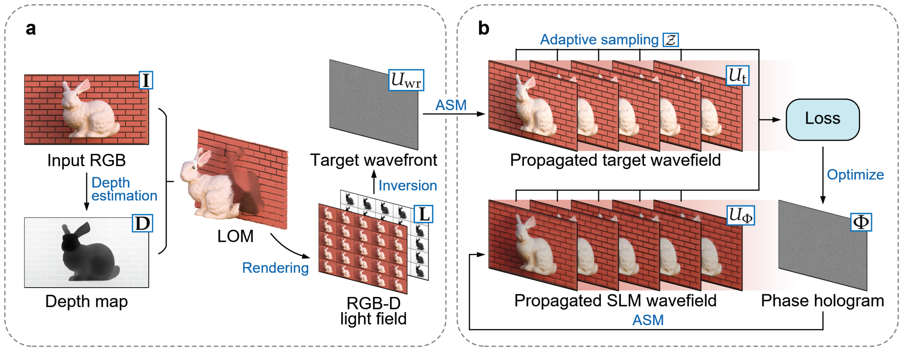
Figure 2.
Optical layout of the phase-only holographic display prototype.
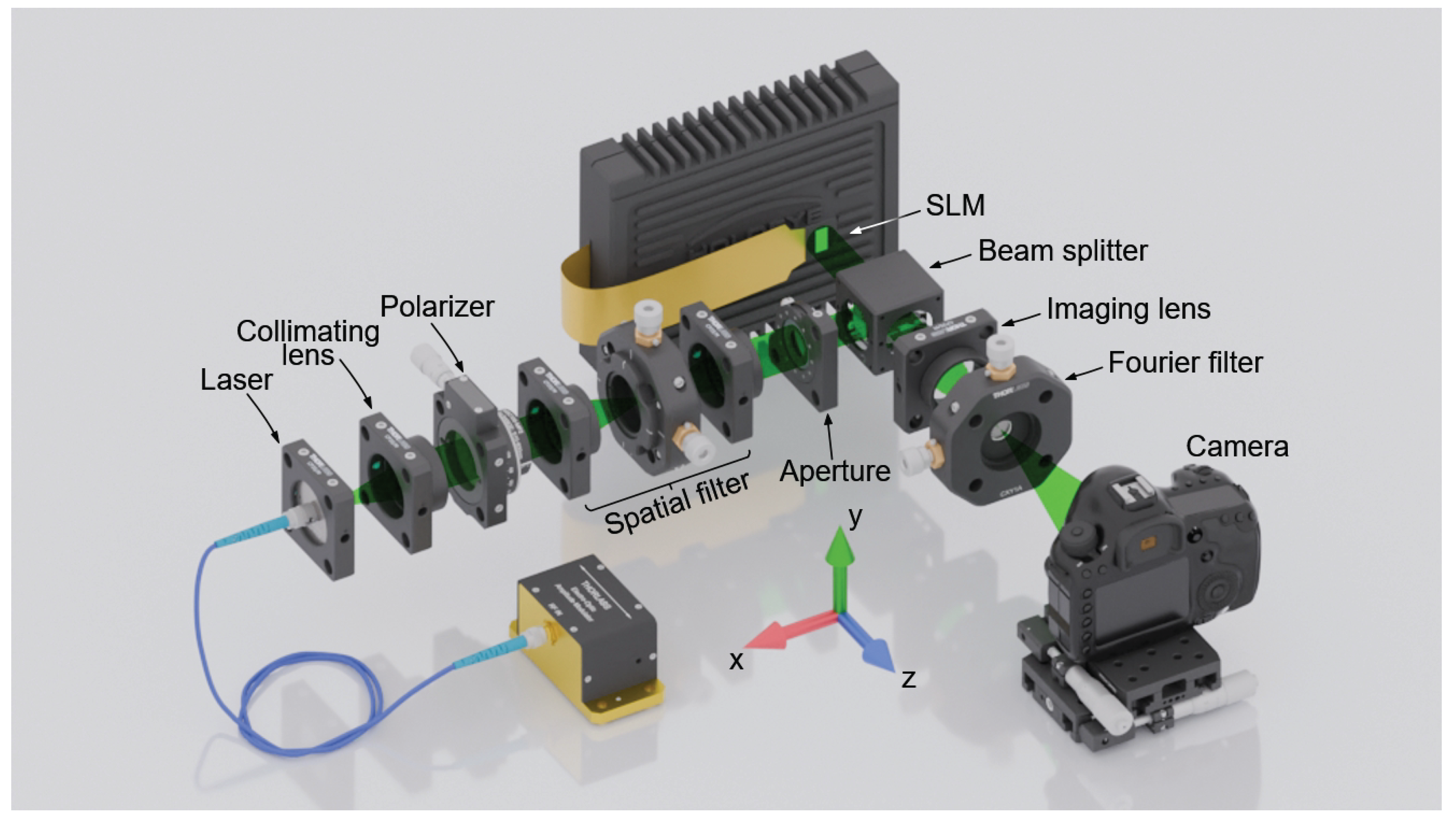
Figure 3.
Comparison of target wavefronts obtained using different light-field generation methods. (a) Input principal-view RGB image, the corresponding ground-truth depth map rendered from the full 3D scene, and the monocular depth map estimated by Depth pro. (b) Visual comparison of target amplitude distributions propagated from the wavefronts constructed using GT-LF and LOM-LF at several representative distances. The GT-LF result is used as the reference. The top-left corner of each subfigure shows the PSNR and SSIM between the LOM-LF-based target amplitude and the GT-LF-based target amplitude, and the bottom-left corner shows the propagation distance relative to the recording plane. (c) PSNR and SSIM curves as functions of propagation distance.
Figure 3.
Comparison of target wavefronts obtained using different light-field generation methods. (a) Input principal-view RGB image, the corresponding ground-truth depth map rendered from the full 3D scene, and the monocular depth map estimated by Depth pro. (b) Visual comparison of target amplitude distributions propagated from the wavefronts constructed using GT-LF and LOM-LF at several representative distances. The GT-LF result is used as the reference. The top-left corner of each subfigure shows the PSNR and SSIM between the LOM-LF-based target amplitude and the GT-LF-based target amplitude, and the bottom-left corner shows the propagation distance relative to the recording plane. (c) PSNR and SSIM curves as functions of propagation distance.
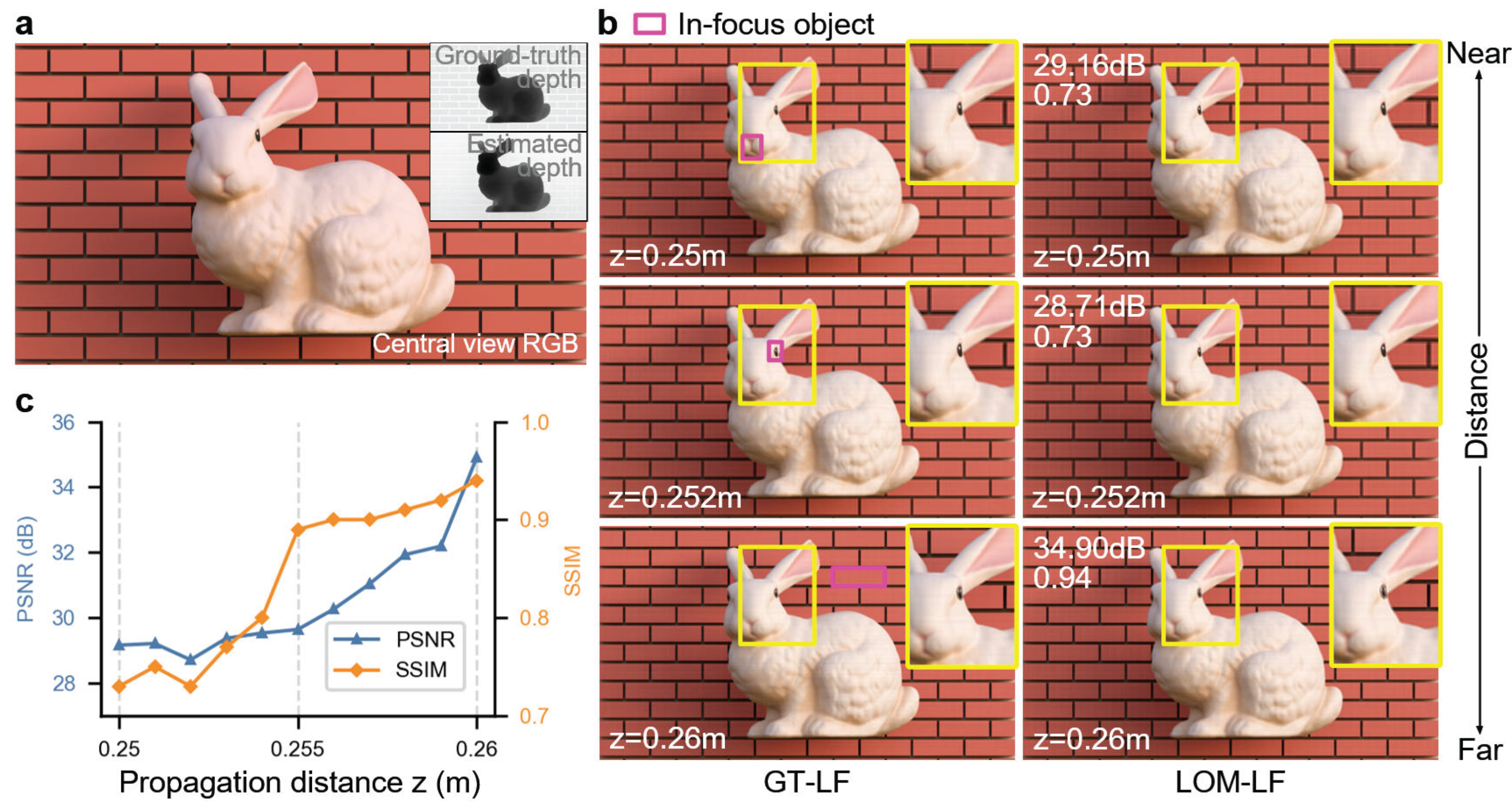
Figure 4.
Influence of different initial phase settings on multi-depth numerical reconstructions. (a) Comparison of multi-depth numerical reconstruction results after 100 iterations using different initial phases: constant phase, half-period random phase, full-period random phase, and the proposed geometrically consistent initial phase. The bottom-right corner of each reconstruction shows the average PSNR and SSIM over all selected reconstruction planes. Enlarged regions highlight local artifact concentration and structured speckle behavior that are not fully reflected by global PSNR/SSIM values. (b) Curves of the multi-depth average PSNR and SSIM versus the number of iterations.
Figure 4.
Influence of different initial phase settings on multi-depth numerical reconstructions. (a) Comparison of multi-depth numerical reconstruction results after 100 iterations using different initial phases: constant phase, half-period random phase, full-period random phase, and the proposed geometrically consistent initial phase. The bottom-right corner of each reconstruction shows the average PSNR and SSIM over all selected reconstruction planes. Enlarged regions highlight local artifact concentration and structured speckle behavior that are not fully reflected by global PSNR/SSIM values. (b) Curves of the multi-depth average PSNR and SSIM versus the number of iterations.
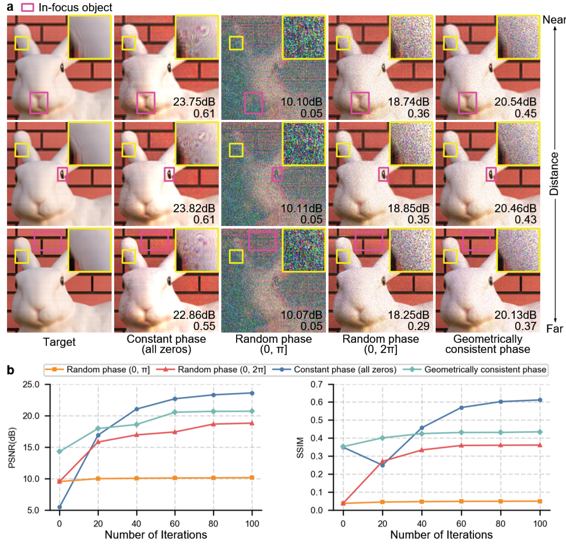
Figure 5.
Influence of different depth-sampling strategies on multi-depth numerical reconstructions. (a) Comparison of multi-depth numerical reconstruction results obtained with fixed depth sampling (FS) and adaptive depth sampling (AS), under an initial number of depth planes of . The bottom-right corner of each result shows the average PSNR and SSIM over all selected reconstruction planes. (b) Bar charts comparing the multi-depth average PSNR and SSIM of the two depth-sampling strategies under different initial numbers of depth planes M; the error bars indicate the standard error over the tested scenes.
Figure 5.
Influence of different depth-sampling strategies on multi-depth numerical reconstructions. (a) Comparison of multi-depth numerical reconstruction results obtained with fixed depth sampling (FS) and adaptive depth sampling (AS), under an initial number of depth planes of . The bottom-right corner of each result shows the average PSNR and SSIM over all selected reconstruction planes. (b) Bar charts comparing the multi-depth average PSNR and SSIM of the two depth-sampling strategies under different initial numbers of depth planes M; the error bars indicate the standard error over the tested scenes.
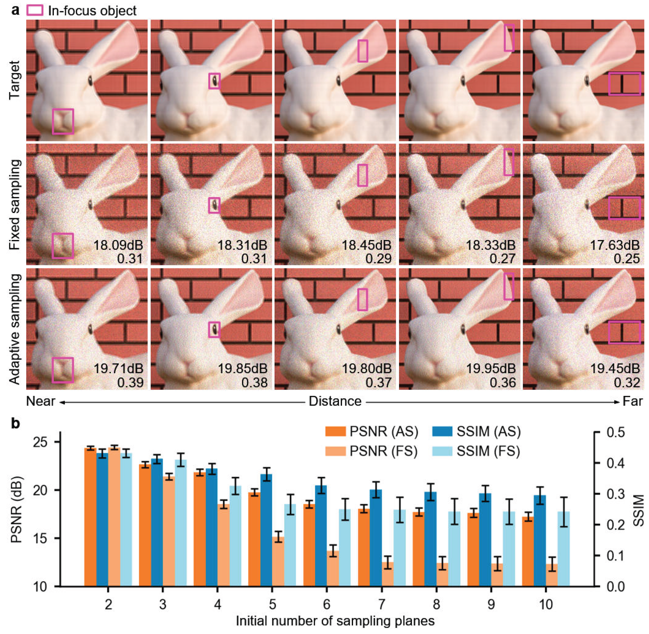
Figure 6.
Comparison of different hologram generation methods in multi-depth numerical reconstructions. (a) Example RGB-D images used for constructing the test scenes. (b)–(d) For three different scenes, multi-depth numerical reconstructions at several representative planes obtained by the layer-based method (LBM), point-based method (PBM), Hogel-Free Holography (HFH), and the proposed method (Ours). For each method, both the overall reconstruction and magnified local details are shown. The bottom indicates the corresponding average PSNR and SSIM over the selected reconstruction planes. The enlarged insets emphasize local crosstalk, occlusion-boundary sharpness, and depth-transition continuity, which are not fully captured by global image-quality metrics alone.
Figure 6.
Comparison of different hologram generation methods in multi-depth numerical reconstructions. (a) Example RGB-D images used for constructing the test scenes. (b)–(d) For three different scenes, multi-depth numerical reconstructions at several representative planes obtained by the layer-based method (LBM), point-based method (PBM), Hogel-Free Holography (HFH), and the proposed method (Ours). For each method, both the overall reconstruction and magnified local details are shown. The bottom indicates the corresponding average PSNR and SSIM over the selected reconstruction planes. The enlarged insets emphasize local crosstalk, occlusion-boundary sharpness, and depth-transition continuity, which are not fully captured by global image-quality metrics alone.
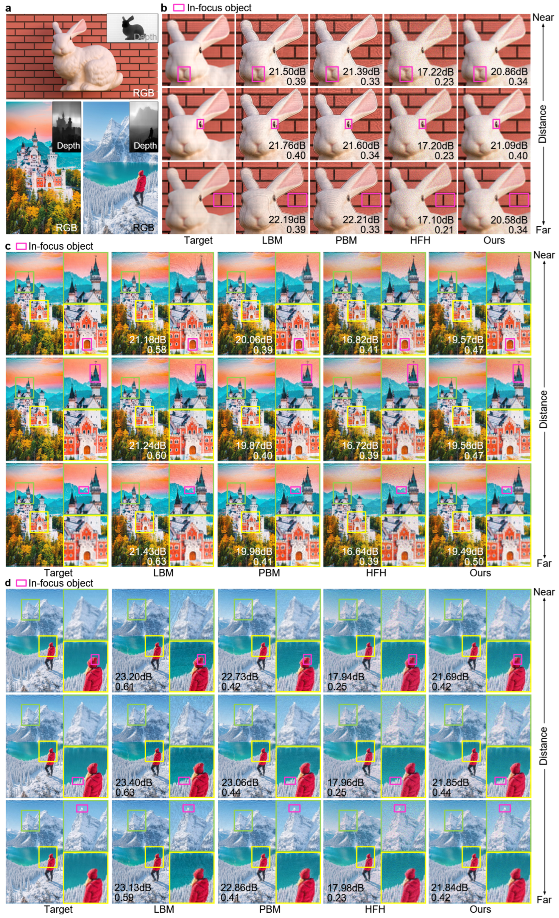
Figure 7.
Multi-depth optical reconstruction comparison between Hogel-Free Holography (HFH) and the proposed method on the holographic display prototype. (a)–(c) Optical reconstruction images of three different test scenes at multiple observation distances, captured by translating the bare CMOS sensor along the optical axis. For each method and each scene, both the overall reconstruction and magnified local details are shown. The optical results are presented as qualitative validation of focus/defocus behavior, depth continuity, and speckle characteristics under the pseudo-color sequential capture protocol.
Figure 7.
Multi-depth optical reconstruction comparison between Hogel-Free Holography (HFH) and the proposed method on the holographic display prototype. (a)–(c) Optical reconstruction images of three different test scenes at multiple observation distances, captured by translating the bare CMOS sensor along the optical axis. For each method and each scene, both the overall reconstruction and magnified local details are shown. The optical results are presented as qualitative validation of focus/defocus behavior, depth continuity, and speckle characteristics under the pseudo-color sequential capture protocol.
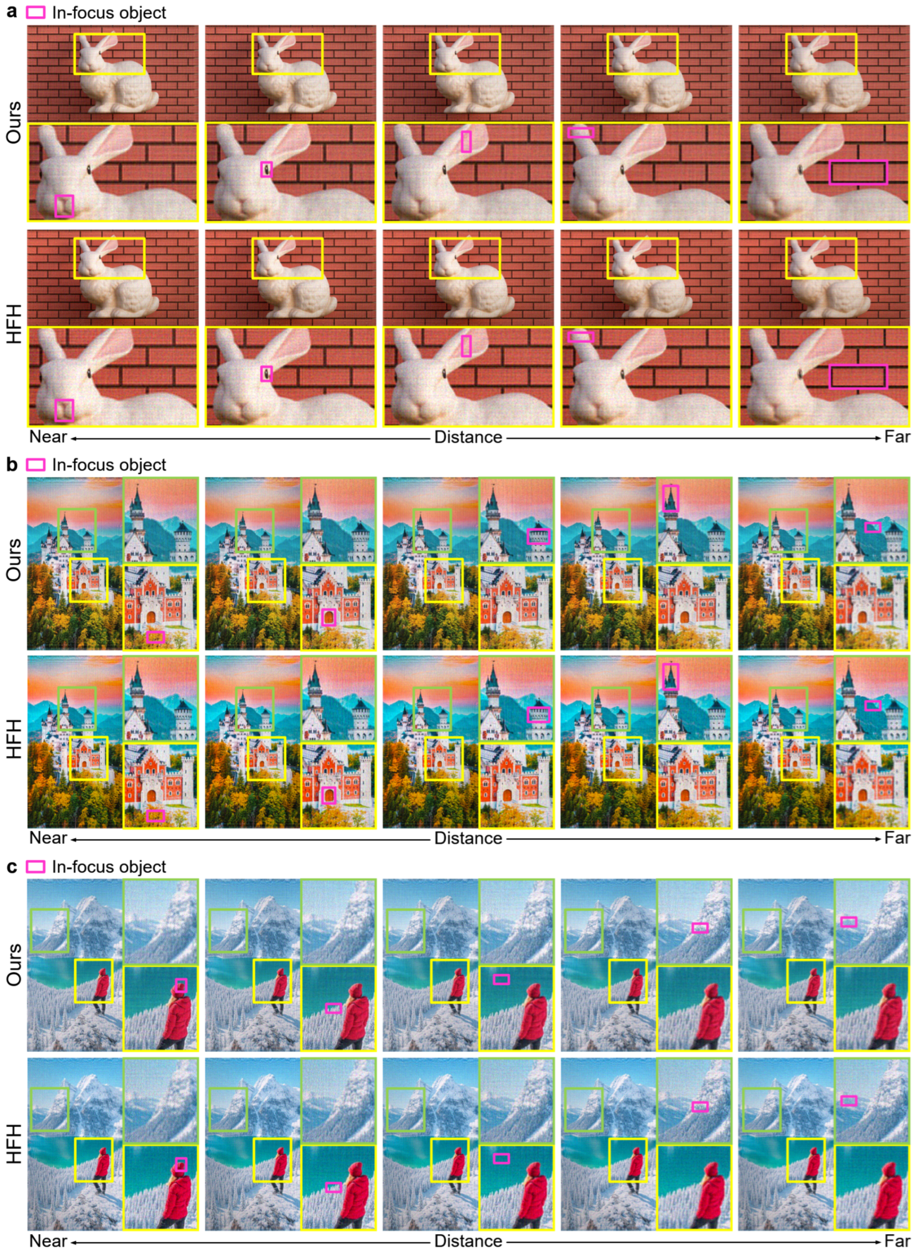

Table 1.
Average total runtime of different hologram generation methods.
| Method | Input | Iterations | Average Runtime (s) |
|---|---|---|---|
| LBM | RGB-D | – | 3.1 |
| PBM | Point cloud | – | 243.7 |
| HFH | RGB-D light-field | 500 | 40.8 |
| Ours | RGB | 100 | 12.9 |
Table 2.
Module-wise runtime breakdown of the proposed method.
| Module | Average Runtime (s) |
|---|---|
| Monocular depth estimation (Depth pro) | 0.6 |
| LOM construction | 0.8 |
| Sparse RGB-D light-field rendering | 1.9 |
| Target wavefront construction | 1.2 |
| Phase iterative optimization | 8.4 |
| Total | 12.9 |
Disclaimer/Publisher’s Note: The statements, opinions and data contained in all publications are solely those of the individual author(s) and contributor(s) and not of MDPI and/or the editor(s). MDPI and/or the editor(s) disclaim responsibility for any injury to people or property resulting from any ideas, methods, instructions or products referred to in the content. |
© 2026 by the authors. Licensee MDPI, Basel, Switzerland. This article is an open access article distributed under the terms and conditions of the Creative Commons Attribution (CC BY) license (http://creativecommons.org/licenses/by/4.0/).
Copyright: This open access article is published under a Creative Commons CC BY 4.0 license, which permit the free download, distribution, and reuse, provided that the author and preprint are cited in any reuse.