

Submitted:
20 March 2026
Posted:
24 March 2026
You are already at the latest version
Abstract
This study presents an approach to forecasting water consumption using the ARIMA (Autoregressive Integrated Moving Average) method, with an additional comparison to the Holt- Winters method [1], [ 2 ], [ 3], [ 4], [ 5 ]. The work was based on a set of historical data representing the monthly water consumption of a specific area in the parish of Cambra, municipality of Vouzela, Portugal, covering a period of five years (2018-2022). Initially, the natural logarithmic transformation was applied to normalise the data [ 6], followed by the Kwiatkowski-Phillips-Schmidt-Shin (KPSS) test to check the stationarity of the time series [ 7]. Differentiation was applied to achieve the necessary stationarity. The Auto-ARIMA method was used to determine the optimal parameters (p,d,q) based on the Akaike Information Criterion (AIC) [ 8], [9]. In addition, the Holt-Winters method was implemented directly, taking advantage of its ability to deal with non-stationary and non-normally distributed series. This method was applied with additive components and Box-Cox transformation [10 ], automatically incorporating the transformation and adjustment processes for seasonality and trend. Both methods were used to forecast water consumption for the 12 months to 2023. After applying Auto-ARIMA, the series was reversed, i.e. differentiated, and exponentially transformed to return to the original values. The performance of both methods was assessed comparatively, using the Mean Absolute Error as a metric [ 11 ], [12]. This study contributes to the efficient management of water resources by providing a robust methodology for forecasting water consumption, with an emphasis on the detailed application of ARIMA and a complementary comparison with Holt-Winters. Throughout this study, both ARIMA and Holt-Winters will be approached as statistical methods that generate models for forecasting data.
Keywords:
ARIMA
; Holt-Winters
; water
; forecast
; sustainability
1. Introduction
The efficient management of water resources is a growing challenge worldwide, especially in the face of climate change and increased demand for water. In this context, accurate forecasting of water consumption becomes a crucial tool for planning and decision-making by water managers. Water consumption in residential areas is influenced by several factors, including seasonal variations, household usage patterns or demographic trends. The complexity of these factors makes forecasting water consumption a significant challenge for local councils as water managers. Advanced statistical methods, such as ARIMA (Autoregressive Integrated Moving Average) or Holt-Winters, have proven effective in forecasting time series in various fields, including water consumption, as they are particularly useful for capturing complex patterns in historical data and projecting future trends. This study focuses on the application of the ARIMA and Holt-Winters methods, using python technology, to forecast monthly water consumption in a specific area of Cambra, in the municipality of Vouzela, as illustrated in Figure 1. The choice of this locality as a case study offers a unique opportunity to examine consumption patterns in a medium-sized Portuguese community, potentially providing knowledge applicable to other nearby regions with similar characteristics. The main objective of this work is to develop and evaluate robust forecasting models that assist in water supply management and planning. By using five years worth of historical data (2018-2022), in addition to forecasting consumption for the following year, a better understanding of the underlying patterns of water consumption in the region is obtained. In addition to the application of statistical methods, this study addresses common challenges in time series analysis, such as data normalisation, stationarity checking and the selection of optimal parameters, specifically for the ARIMA method. The methodology applied aims to provide a replicable approach that can be adapted and applied in other water resource management contexts. The following sections present a review of the relevant literature, details of the methodologies employed for forecasting the data through experimental work, a discussion of the results obtained and a brief approach to the implications of this study for water resources management. Finally, directions for future work will be indicated, including the recommendation to implement telemetry with LoRaWAN technology [13]. The rest of the article is organised as follows. Section 2 presents the related work. Section 3 describes the experimental work. Section 4 deals with the results observed during the application of the methods and, finally, the conclusions and future work are presented in Section 5.
2. Related Work
The ARIMA (Autoregressive Integrated Moving Average) and Holt-Winters methods have been widely used in various fields to forecast time series, demonstrating their versatility and effectiveness. This section presents an overview of some studies that have applied these statistical methods in different contexts, providing a comparative basis for the present work. In the field of energy, Ediger and Akar (2007) applied ARIMA methods and SARIMA (Seasonal AutoRegressive Integrated Moving Average), an extension of ARIMA that specifically deals with seasonal components in time series, to forecast primary energy consumption in Turkey [14]. The results of the forecast indicated that the growth rate of energy needs will decrease, with the exception of wood and vegetable waste, emphasising the relevance of renewable sources to guarantee energy security. In the electricity sector, Contreras et al. (2003) used ARIMA methods to forecast electricity prices in competitive markets. Tests carried out in the Spanish and California markets revealed average daily errors of 5-10%, demonstrating the applicability of ARIMA in volatile markets [15]. For natural gas consumption, Taspinar et al. (2013) compared ARIMA methods with approaches based on Fourier series expansion. Although ARIMA was outperformed in this case, the study emphasises the importance of considering seasonal variations and temperature feedback in energy consumption forecasts [16]. The COVID-19 pandemic has prompted several studies using ARIMA to forecast cases. Chakraborty and Ghosh (2020) applied the method to forecast the number of cases in five severely affected countries. Similarly, Zeroual et al. (2020) compared ARIMA with Machine Learning (NARNN - Nonlinear Autoregression Neural Network) and (LSTM - Long-short term memory) approaches to predict cases in European countries [17,18]. Maleki et al. (2020) proposed an algorithm to calculate the best ARIMA parameters per country, analysing 145 countries in six geographical regions. This study highlighted the relationship between the behaviour of the virus and population variables, suggesting the incorporation of factors such as humidity and culture in future models [19]. In the financial field, Mondal et al. (2014) evaluated the effectiveness of ARIMA in forecasting Indian stock prices, achieving an accuracy of over 85 per cent in various sectors. This study demonstrates the applicability of ARIMA in financial markets, although it emphasises the need for more specific methods for certain sectors [20]. In the field of aviation, Alhindi et al. (2021) used ARIMA to predict visibility based on meteorological data, a crucial factor for air safety. The promising results suggest exploring Machine Learning techniques to further improve forecast accuracy [21]. In the context of agricultural price forecasting, the study applied the ARIMA method to forecast potato prices in Turkey, demonstrating that ARIMA outperformed other methods, such as Holt-Winters, in accuracy. The results indicate that ARIMA is effective in modelling time series, in this case prices, highlighting its relevance for formulating economic policies. This work contributes to the literature by highlighting the importance of price stability in agriculture [22]. Still in the area of time series forecasting, Koehler et al. (2001) explored new methods based on the multiplicative Holt-Winters method, which is fundamental for dealing with data that has a trend and seasonality. The research demonstrated that the forecast error variance can be adjusted to reflect these characteristics, improving forecast accuracy. The results indicate that the correct choice of model is crucial, especially in series with an upward trend, which can have significant implications in a number of practical applications [23]. These studies demonstrate the versatility and effectiveness of statistical methods in various fields, from energy and public health to finance and aviation. The successful application of ARIMA in forecasting energy consumption, as demonstrated by Ediger and Akar (2007), provides a solid basis for our approach to forecasting water consumption. Furthermore, the lessons learnt from the COVID-19 case study, particularly the importance of considering regional and seasonal factors, can be applied to our water consumption analysis. Maleki et al.’s (2020) methodology for optimising ARIMA parameters by region offers important insights for the localised approach in Cambra, Portugal. This work builds on these successful applications of ARIMA and Holt-Winters, adapting them to the specific context of water consumption forecasting, with the aim of contributing to more efficient management of water resources.
3. Experimental Work
The study is based on a set of water consumption data, in cubic meters (m³), from 2018 to 2022, from 41 meters in a specific area of Confulcos, in the parish of Cambra, in the municipality of Vouzela. The first step in processing the data was to build a dataset, as shown in Table 1, and then a time series.
Using a list previously generated with the monthly data extracted from the dataset, and the indices generated for this purpose, we can see in Figure 2 the series in the form of a line graph, where we can see an upward trend and a pattern of higher consumption at certain periods of each year.
In Figure 3, after decomposing the series, we can clearly see the trend and seasonality, as well as the residuals. These residuals correspond to the part of the series that is not explained by the trend and seasonality. The analysis reveals that the series shows a seasonal pattern, with variations over time, and an upward trend, showing an increase in water consumption, particularly in the summer months.
These steps proved crucial to understanding the time series. The visual analysis allowed us to identify a clear trend in the series, indicating that the average does not oscillate around a constant value. It was also possible to detect a recurring pattern of consumption over the period analysed. With the aim of drawing up a forecast using the ARIMA method in mind, the next step was to assess whether the data had an approximately normal distribution. Although not strictly necessary for the application of the model, this check is advisable because it can help validate the suitability of the model, ensuring that the residuals are random and do not show systematic patterns, which is fundamental for the reliability of the forecasts. However, looking at the graph shown in Figure 4 raised some uncertainties about this normality.
One of the techniques for checking the normality of data is to perform the Shapiro-Wilk test, with a significance level of 5% (commonly used). This test is recommended for a set of small and moderate samples, but it maintains high precision even at higher numbers (n < 100), compared to other tests such as Kolmogorov-Smirnov with Lilliefors correction [24,25]. The Shapiro–Wilk (SW) test is a well-known method to assess whether a sample comes from a normally distributed population. It is based on the following statistic:
where:
- W is the Shapiro–Wilk test statistic,
- n is the number of observations in the sample,
- are the ordered sample values such that ,
- are constants derived from the means, variances, and covariances of the order statistics of a sample from the standard normal distribution,
- are the original (unordered) sample values,
- is the mean of the sample.
The test provides a p-value, which is the probability of obtaining a result as extreme as the one observed, assuming that the null hypothesis (of normality) is true [26]. In this case, the p-value was found to be less than the significance level (0.05), which leads to the rejection of the null hypothesis and the acceptance of the alternative hypothesis, indicating that the distribution is not normal. In order to normalise the distribution of the data, we chose to apply a natural logarithmic transformation (base ‘e’). This choice was based on the fact that the series contains only positive integers, and this transformation is effective in reducing variance and improving normality. After applying the logarithmic transformation, the Shapiro-Wilk test was performed again. The new result ( 0.051) indicated that the distribution of the transformed data is now approximately normal, which is reflected in Figure 5.
In addition to normalising the data, applying the ARIMA method requires the series to be stationary. This means that its statistical properties, such as mean and variance, must remain constant over time, without exhibiting trends or seasonal patterns. Although the initial decomposition revealed an increasing trend and a periodic pattern in the series, the Kwiatkowski-Phillips-Schmidt-Shin (KPSS) test was carried out to confirm stationarity. The result of the test indicated that the series was not stationary, as the test statistic exceeded the critical value, leading to the rejection of the null hypothesis of stationarity. To make the series stationary, the differentiation technique was applied. This method creates a series by calculating the difference between consecutive values, subtracting each value from its successor [27]. This approach helps to eliminate trends and stabilise the average. Figure 6 shows the graph of the series after differentiation, where you can see that the trend has been removed and the average oscillates around a constant value, indicating that the series has become stationary.
After processing the series, ensuring that it met the necessary requirements for applying the ARIMA method, we proceeded to implement the method itself on the differentiated series.
3.1. ARIMA and SARIMA Method
Once the series had been processed, ensuring that it met the necessary requirements for the application of the ARIMA method, the method itself was implemented on the differentiated series. The ARIMA method has three parameters (p, d, q) and is often written as ARIMA(p, d, q), where p represents the order of the autoregressive component, d is the number of differentiations required to obtain a stationary ARMA(p, q) model, and q corresponds to the order of the moving average component. The general ARIMA(p, d, q) formula is expressed by a lag operator [28], represented as:
where the characteristic operators are:
and
The definitions of the symbols are:
- is the estimate of the autoregressive component parameter,
- is the estimate of the moving average component parameter,
- is the differencing operator,
- B is the lag operator,
- is a purely random process with zero mean and variance (white noise).
Crucial parameters were considered, such as the number of combinations for each parameter and the monthly seasonal period. We chose to use Auto-ARIMA, a method that automatically combines various regression orders (p), moving averages (q) and degrees of differentiation (d), with the aim of identifying the most suitable model. It is important to emphasise that Auto-ARIMA is an algorithm that can automatically select the best model generated by the ARIMA or SARIMA methods for a time series. When selecting a SARIMA method, it incorporates seasonality, resulting in a combination of the parameters of the standard method (p,d,q) with the seasonal parameters (P,D,Q)m, where m represents the seasonal period [29]. The SARIMA(p,d,q)(P,D,Q)m method represented as:
where the seasonal operators are:
and
The definitions of the symbols are:
- is the estimate of the non-seasonal autoregressive component parameter,
- is the estimate of the seasonal autoregressive component parameter,
- is the estimate of the non-seasonal moving average component parameter,
- is the estimate of the seasonal moving average component parameter,
- B is the lag operator,
- d and D are the orders of non-seasonal and seasonal differencing, respectively,
- m is the number of periods per season,
- is a purely random process with zero mean and variance (white noise).
Since the method was applied to an already differentiated series, Auto-ARIMA identified the optimal model without the need for additional degrees of differentiation, as can be seen in Figure 7.
The report produced by the Auto-ARIMA method identified the most appropriate model using the Akaike Information Criterion (AIC). The AIC, is a statistical tool that assesses the relative quality of statistical models for a specific data set, balancing the accuracy of the fit with the complexity of the model [29,30]. The AIC represented as:
where:
- L is the maximized likelihood of the model,
- k is the number of estimated parameters in the model.
Figure 8 shows the detailed results of the SARIMA method chosen, which includes seasonality. This method integrates autoregressive and moving average elements, with an order (1,0,1) for the non-seasonal component and an order (3,0,0) for the seasonal component, considering a 12-month seasonal cycle. Specifically, for the non-seasonal component, we have an autoregressive order (p) of 1, a degree of differentiation (d) of 0, and a moving average order (q) of 1. For the seasonal component, the seasonal autoregressive order (P) is 3, the seasonal degree of differentiation (D) is 0, and the seasonal moving average order (Q) is 0. The seasonal period (s) is 12 months. The choice of this particular model suggests that it provides the best balance between fit to the data and complexity, as assessed by the AIC. This indicates that the model efficiently captures the fundamental characteristics of the time series, including trends, seasonal patterns and other fluctuations, while avoiding overfitting the data.
After modeling the series, the next step was to extract the residuals and analyze the autocorrelation between these data. In the context of time series, residuals are the differences between the observed values and the values predicted by the model. The analysis of these residuals is crucial, as it examines the relationship of the residuals within the same set, all associated with the water consumption variable. If the model is suitable, the residuals should be random and show no systematic patterns. It is important to note that the forecast is generated from these residuals, as they are derived from a series that has been properly treated and modeled. Analysis of the residuals made it possible to validate the model produced by the Auto-ARIMA method. This validation was possible because the model passed the normality test and, as mentioned above, the evaluation of autocorrelation and partial autocorrelation. The graphs presented illustrate that the residuals in both the Autocorrelation Function (Figure 9) and the Partial Autocorrelation Function (Figure 10) do not exhibit significant autocorrelation. This is evidenced by the fact that the bars, which represent periods in the time domain, remain within the 95% confidence interval.
This observation suggests that the model was able to efficiently capture the temporal structure of the data.
Once the series of residuals had passed the tests, we proceeded to forecast the data for the next 12 months, corresponding to the year 2023. It is important to note that the residuals are on a reduced scale, resulting from the transformations applied to the original series - first the logarithmic transformation and then the differentiation. Consequently, the forecast is also on this reduced scale, making it necessary to revert all the data to the original scale. The process of reversing the differentiation involves the reverse procedure to the one applied initially. Instead of subtracting consecutive values, each value of the differentiated forecast is added to the corresponding value of the non-differentiated series. This process is carried out iteratively, starting with the addition of the first value of the differentiated series to the last known value of the non-differentiated series. After reversing the differentiation, it is still necessary to apply the exponential function to the series, since the logarithmic function was initially applied to normalize the distribution, as indicated by the Shapiro-Wilk test. Figure 11 shows a graphical view of the consumption forecast for 2023, highlighted in red, after the data has been processed to return to the initial scale.
The numerical results of the forecast, obtained by the ARIMA method considered optimal according to the Akaike Information Criterion (AIC), are presented in tabular format together with the results of the Holt-Winters method for comparative purposes.
3.2. Holt-Winters
After forecasting water consumption for 2023 using the ARIMA method, the Holt-Winters method was applied to the original series, before the transformations carried out for the ARIMA method. Forecasting using the Holt-Winters additive method, also known as triple exponential smoothing, was chosen due to the observation of a constant seasonality in the time series. This method uses three fundamental equations to model the level, trend and seasonality of the series [28,31], represented as:
Level:
Trend:
Seasonality:
Forecast:
The definitions of the symbols are:
- represents the level of the series,
- represents the trend,
- is the seasonal component,
- is the observed value at time t,
- , , are the smoothing parameters,
- m is the number of observations per seasonal cycle,
- h is the forecast horizon,
- .
The additive method is more appropriate when the amplitude of seasonal fluctuations remains relatively constant over time, regardless of the overall level of the series. In contrast, the multiplicative method would be preferable if the magnitude of seasonal variations increased proportionally over the series. While trend and seasonality follow similar principles to those discussed in the application of the ARIMA method, the Holt-Winters method introduces the concept of “level”. This is characterized as a weighted average that gives greater importance to the most recent data. The “level” is updated at each iteration, taking into account the trend and seasonality of the series. Although this method does not build a model with parameters (p,d,q)(P,D,Q) like SARIMA, it does generate a model with specific parameters: level smoothing (), trend smoothing () and seasonal smoothing (). These parameters control the rate at which the model adapts to changes in the level, trend and seasonal pattern of the series, respectively. Figure 12 illustrates that the forecast (represented by the black line) shows greater similarity to the immediately preceding period than to any other observed period, due to the influence of the “level” variable.
In the following Table 2 shows the actual values for the year 2023, the values predicted by the ARIMA method for the same year, as well as the values predicted by the Holt-Winters method for the same period. The comparison between three sets of data for the year 2023, i.e. the actual values observed, the forecasts generated by the ARIMA method and the forecasts produced by the Holt-Winters method. This Table 2 allows for a direct comparative analysis between the data actually recorded and the projections made by both forecasting methods, making it easier to assess the accuracy and effectiveness of each modeling approach.
4. Results
The section discussing the results focuses on the comparative analysis of the water consumption forecasts obtained using the Holt-Winters and ARIMA statistical methods. Figure 13 shows a graph overlaying the forecasts generated by both methods with the actual values observed. This visualization reveals that the Holt-Winters method (represented by the blue line) shows a lower error in its forecasts compared to the ARIMA method (red line). The superior effectiveness of the Holt-Winters method can be attributed to the inconsistency in the seasonality and trend patterns observed in previous years, possibly influenced by the global COVID-19 pandemic, which significantly altered consumption habits during 2020 and 2021. The Holt-Winters method manages to produce forecasts that are closer to the real values (green line) due to its characteristic of giving greater weight to the most recent data in the forecast equation. This approach allows for faster adaptation to recent changes in consumption patterns.
By graphing the actual time series (2018-2022), together with the actual consumption figures for the year 2023 and the forecasts generated by both statistical methods, in Figure 14, it becomes clear that the Holt-Winters method produced results closer to the observed reality. The line graph shows a clear visual comparison between the original time series from 2018 to 2022, actual consumption figures recorded in 2023, the forecasts generated by the ARIMA method and the forecasts produced by the Holt-Winters method. This graphical representation allows for an immediate comparative analysis, highlighting the superior accuracy of the Holt-Winters method forecasts compared to the ARIMA method when compared to the actual consumption data in 2023.
To conclude the analysis, we evaluated the accuracy of both models generated by the statistical methods SARIMA and Holt-Winters, using two complementary metrics: the Mean Absolute Error (MAE) and the Mean Squared Error (MSE). These evaluation metrics provide different perspectives on the quality of the predictions, there by enabling a more robust analysis of the models performance [32,33,34].
Evaluation Metrics
The Mean Absolute Error (MAE) is calculated as:
The Mean Squared Error (MSE) is calculated as:
where:
- are the observed values,
- are the values predicted by the model,
- n is the total number of observations.
Characteristics and Complementarity of the Metrics
These two metrics complement each other in the evaluation of prediction models:
-
MAE: Measures the average magnitude of the errors in absolute terms, treating all errors equally. It is expressed in the same unit as the original variable (cubic meters of water), which facilitates direct interpretation.
- -
- It is less sensitive to outliers, providing a more robust measure of error.
- -
- It offers a direct interpretation of the average error magnitude.
-
MSE: Measures the average of the squared errors, penalizing larger errors more strongly. It is expressed in the square of the original unit.
- -
- It is more sensitive to outliers and large errors, which can be useful when such errors have a significant impact on the application.
- -
- It quadratically penalizes larger deviations, which is particularly useful when large errors are especially undesirable.
The combined use of these metrics allows for a more complete evaluation of the predictive quality of the models, capturing different aspects of their performance.
Analysis of the Results
Figure 15 and Figure 16 show a quantitative comparison of the forecasting effectiveness of the methods used in this study:
- For the MAE, the Holt-Winters method achieved a value of 59.45, whereas SARIMA presented a value of 81.97.
- For the MSE, the Holt-Winters method obtained a value of 4863.43, while SARIMA showed a value of 10132.71.
In both metrics, lower values indicate better model performance. The results clearly show that the Holt-Winters method outperformed SARIMA in both evaluation metrics:
- 1.
- The lower MAE (59.45 vs. 81.57) indicates that, on average, the Holt-Winters forecasts deviate less from the actual values in absolute terms.
- 2.
- The substantially lower MSE (4863.43 vs. 10132.71) suggests that Holt-Winters not only produces smaller errors on average, but also has a lower tendency to generate large errors, which are strongly penalized by the quadratic nature of MSE.
The proportional difference between the models is even more pronounced in the MSE (approximately 52% lower for Holt-Winters) than in the MAE (approximately 27% lower), indicating that the Holt-Winters method is particularly effective in reducing large-magnitude errors.
The joint analysis of MAE and MSE provides robust evidence that the Holt-Winters method demonstrates superior predictive capability when compared to the SARIMA method for the dataset analyzed. This superiority is consistent across both evaluation metrics, reinforcing the confidence in selecting Holt-Winters as the most suitable model for forecasting water consumption in this specific context.
This conclusion highlights the importance of appropriately selecting forecasting methods and generating models in time series analysis, especially in practical applications such as water resource management. The use of multiple complementary evaluation metrics, such as MAE and MSE, enriches the analysis and increases confidence in the obtained conclusions.
5. Conclusions and Future Work
This study demonstrated the successful application of ARIMA and Holt-Winters methods in forecasting monthly water consumption in Cambra, Vouzela. The detailed methodology for ARIMA, including logarithmic transformation, KPSS stationarity testing, differentiation, and (automatic) parameter selection via Auto-ARIMA, provided a robust approach to handling the complexities of the water consumption time series. The comparison between ARIMA and Holt-Winters yielded valuable conclusions regarding the relative effectiveness of these methods for this specific dataset. The use of the Mean Absolute Error (MAE) and Mean Squared Error (MSE) as an evaluation metrics allowed for an objective comparison, highlighting the strengths and limitations of each approach. Likely due to changes in water consumption habits in 2020 and 2021, influenced by the COVID-19 pandemic, the Holt-Winters method proved more effective, as its characteristic of assigning greater weight to more recent data made it better suited for forecasting. The results obtained have significant implications for water resource management in the parish of Cambra and potentially in other similar regions. However, Auto-ARIMA may prove to be the more effective method in other nearby regions, as the choice will always depend on the constructed time series, with seasonality playing a particularly relevant role. The generated forecasts can assist municipal managers in more efficiently planning water supply, providing advance information on periods of higher consumption. Based on these insights, it is possible to adjust distribution capacity, optimise resource allocation—such as personnel and infrastructure—and make informed decisions regarding maintenance or future investments. Additionally, forecast-based planning can help identify and mitigate potential water scarcity risks, preventing wastage and promoting the sustainability of water resources. For future work, it is recommended to implement telemetry using LPWAN (Low Power Wide Area Network) technology for real-time data collection, enabling more frequent and accurate updates to statistical methods, as well as developing an early warning system based on forecasts to identify potential anomalies in water consumption. This research makes a significant contribution to the field of water resource management, providing a replicable methodology and valuable insights into water consumption patterns. The continuous refinement and expansion of these models have the potential to substantially enhance the efficiency and sustainability of water usage in both urban and rural contexts.
Author Contributions
Conceptualization, J.R. and S.S.; methodology, J.R., S.S. and A.V.; software, J.R. and A.V.; validation, J.R., S.S. and A.V.; formal analysis, J.R. and S.S.; investigation, J.R. and A.V.; resources, S.S., A.V. and F.C.P.; data curation, J.R. and F.C.P.; writing—original draft preparation, J.R. and S.S.; writing—review and editing, J.R., S.S., A.V. and F.C.P.; visualization, J.R. and S.S.; supervision, S.S. and A.V.; project administration, S.S.; funding acquisition, S.S. and A.V. All authors have read and agreed to the published version of the manuscript.
Acknowledgments
Authors would like to thank the civil protection entity.
Conflicts of Interest
The authors declare no conflict of interest.
Abbreviations
The following abbreviations are used in this manuscript:
| AIC | Akaike Information Criterion |
| ARIMA | Autoregressive Integrated Moving Average |
| KPSS | Kwiatkowski-Phillips-Schmidt-Shin |
| LPWAN | Low Power Wide Area Network |
| LSTM | Long-short term memory |
| MAE | Mean Absolute Error |
| MSE | Mean Squared Error |
| NARNN | Nonlinear Autoregression Neural Network |
| SARIMA | Seasonal AutoRegressive Integrated Moving Average |
References
- IBM. What are ARIMA models? Available online: https://www.ibm.com/think/topics/arima-model. Accessed: 2024-11-17.
- Khan, S.; Alghulaiakh, H. ARIMA Model for Accurate Time Series Stocks Forecasting. International Journal of Advanced Computer Science and Applications 2020, 11. [CrossRef]
- Newbold, P. ARIMA model building and the time series analysis approach to forecasting. Journal of Forecasting 1983, 2, 23–35, [https://onlinelibrary.wiley.com/doi/pdf/10.1002/for.3980020104]. [CrossRef]
- Chatfield, C. The Holt-Winters Forecasting Procedure. Journal of the Royal Statistical Society. Series C (Applied Statistics) 1978, 27, 264–279.
- Chatfield, C.; Yar, M. Holt-Winters Forecasting: Some Practical Issues. Journal of the Royal Statistical Society. Series D (The Statistician) 1988, 37, 129–140.
- Assis, J.P.D.; Lima, I.R.P.D.; França, J.D.A.; Sousa, R.P.D.; Linhares, P.C.F.; Custódio, T.N.; Sousa, R.P.D.; Rodrigues, W.M. Transformação de Dados Aplicada à Estatística; Pantanal Editora: Brasil, 2023. [CrossRef]
- Hobijn, B.; Franses, P.H.; Ooms, M. Generalizations of the KPSS-test for stationarity. Statistica Neerlandica 2004, 58, 483–502, [https://onlinelibrary.wiley.com/doi/pdf/10.1111/j.1467-9574.2004.00272.x]. [CrossRef]
- Luo, L.; He, K.; Wu, W.; Taylor, J.M. Using information criteria to select smoothing parameters when analyzing survival data with time-varying coefficient hazard models. Statistical Methods in Medical Research 2023, 32, 1664–1679, PMID: 37408385. [CrossRef]
- Cavanaugh, J.E.; Neath, A.A. The Akaike information criterion: Background, derivation, properties, application, interpretation, and refinements. WIREs Computational Statistics 2019, 11, e1460, [https://wires.onlinelibrary.wiley.com/doi/pdf/10.1002/wics.1460]. [CrossRef]
- Sakia, R.M. The Box-Cox Transformation Technique: A Review. Journal of the Royal Statistical Society. Series D (The Statistician) 1992, 41, 169–178.
- Willmott, C.J.; Matsuura, K. Advantages of the mean absolute error (MAE) over the root mean square error (RMSE) in assessing average model performance. Climate Research 2005, 30, 79–82. [CrossRef]
- Chai, T.; Draxler, R.R. Root mean square error (RMSE) or mean absolute error (MAE)? – Arguments against avoiding RMSE in the literature. Geoscientific Model Development 2014, 7, 1247–1250. [CrossRef]
- Lora Alliance. LoRaWAN transforms businesses by connecting wireless IoT sensors simply and affordably. Accessed: 2024-12-19.
- Ediger, V.S.; Akar, S. ARIMA forecasting of primary energy demand by fuel in Turkey. Energy Policy 2007, 35, 1701–1708. [CrossRef]
- Contreras, J.; Espinola, R.; Nogales, F.; Conejo, A. ARIMA models to predict next-day electricity prices. IEEE Transactions on Power Systems 2003, 18, 1014–1020. [CrossRef]
- Yukseltan, E.; Yucekaya, A.; Bilge, A.H.; Agca Aktunc, E. Forecasting models for daily natural gas consumption considering periodic variations and demand segregation. Socio-Economic Planning Sciences 2021, 74, 100937. [CrossRef]
- Sahai, A.K.; Rath, N.; Sood, V.; Singh, M.P. ARIMA modelling & forecasting of COVID-19 in top five affected countries. Diabetes & Metabolic Syndrome: Clinical Research & Reviews 2020, 14, 1419–1427. [CrossRef]
- İsmail Kırbaş.; Sözen, A.; Tuncer, A.D.; Şinasi Kazancıoğlu, F. Comparative analysis and forecasting of COVID-19 cases in various European countries with ARIMA, NARNN and LSTM approaches. Chaos, Solitons & Fractals 2020, 138, 110015. [CrossRef]
- Hernandez-Matamoros, A.; Fujita, H.; Hayashi, T.; Perez-Meana, H. Forecasting of COVID19 per regions using ARIMA models and polynomial functions. Applied Soft Computing 2020, 96, 106610. [CrossRef]
- Mondal, P.; Shit, L.; Goswami, S. Study of effectiveness of time series modeling (ARIMA) in forecasting stock prices. International Journal of Computer Science, Engineering and Applications 2014, 4, 13.
- Salman, A.G.; Kanigoro, B. Visibility Forecasting Using Autoregressive Integrated Moving Average (ARIMA) Models. Procedia Computer Science 2021, 179, 252–259. 5th International Conference on Computer Science and Computational Intelligence 2020, . [CrossRef]
- Şahinli, M.A. Potato Price Forecasting with Holt-Winters and ARIMA Methods: A Case Study. American Journal of Potato Research 2020, 97, 336–346. Published: 2020/08/01, . [CrossRef]
- Koehler, A.B.; Snyder, R.D.; Ord, J. Forecasting models and prediction intervals for the multiplicative Holt–Winters method. International Journal of Forecasting 2001, 17, 269–286. [CrossRef]
- Mishra, P.; Pandey, C.M.; Singh, U.; Gupta, A.; Sahu, C.; Keshri, A. Descriptive statistics and normality tests for statistical data. Annals of Cardiac Anaesthesia 2019, 22, 67–72. [CrossRef]
- Hanusz, Z.; Tarasińska, J. Normalization of the Kolmogorov–Smirnov and Shapiro–Wilk tests of normality. Biometrical Letters 2015, 52. [CrossRef]
- Wasserstein, R.L.; Lazar, N.A. The ASA Statement on p-Values: Context, Process, and Purpose. The American Statistician 2016, 70, 129–133, [. [CrossRef]
- Fattah, J.; Ezzine, L.; Aman, Z.; Moussami, H.E.; Lachhab, A. Forecasting of demand using ARIMA model. International Journal of Engineering Business Management 2018, 10, [. [CrossRef]
- Markovska, M.; Bučkovska, A.; Taskovski, D. Comparative study of ARIMA and Holt-Winters statistical models for prediction of energy consumption. 09 2016.
- Hyndman, R.J.; Khandakar, Y. Automatic Time Series Forecasting: The forecast Package for R. Journal of Statistical Software 2008, 27, 1–22. [CrossRef]
- Akaike, H. A new look at the statistical model identification. IEEE Transactions on Automatic Control 1974, 19, 716–723. [CrossRef]
- Gardner Jr., E.S. Exponential smoothing: The state of the art. Journal of Forecasting 1985, 4, 1–28. [CrossRef]
- Hyndman, R.; Athanasopoulos, G. Forecasting: principles and practice; OTexts, 2018.
- Karunasingha, D.S.K. Root mean square error or mean absolute error? Use their ratio as well. Information Sciences 2022, 585, 609–629.
- Robeson, S.M.; Willmott, C.J. Decomposition of the mean absolute error (MAE) into systematic and unsystematic components. PloS one 2023, 18, e0279774.
Figure 1.
Graphical Abstract.
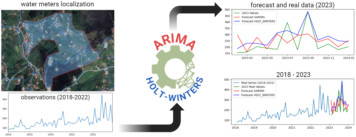
Figure 2.
Series: Original Plot.
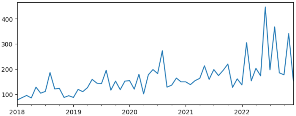
Figure 3.
Series decomposition: trend, seasonality and white noise.
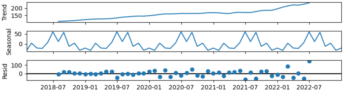
Figure 4.
Shapiro-Wilk: Normality test plot.
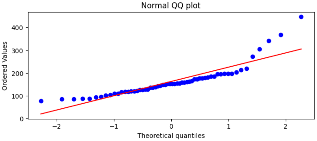
Figure 5.
Shapiro-Wilk: Normality test plot after logarithmic transformation.
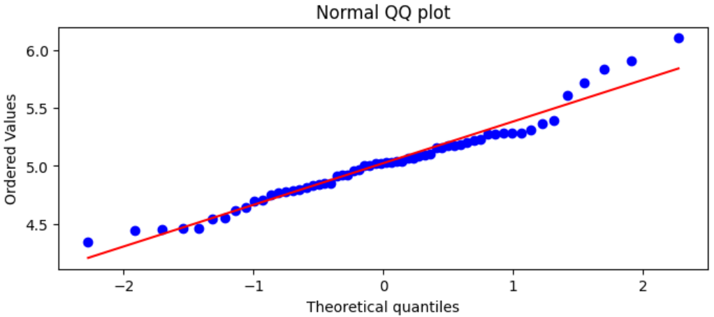
Figure 6.
Series plot after the KPSS method applied.
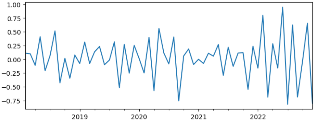
Figure 7.
Creation model after application ARIMA method.
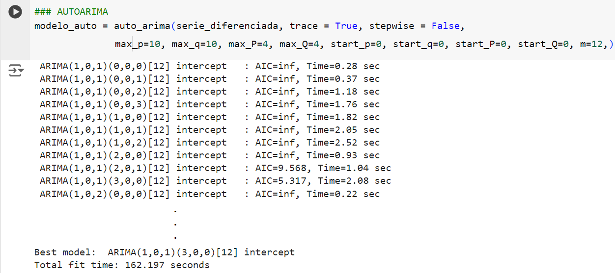
Figure 8.
Best model generated according AIC.
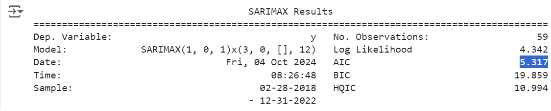
Figure 9.
Autocorrelation: Periods in the time domain, remain within the 95% confidence interval.
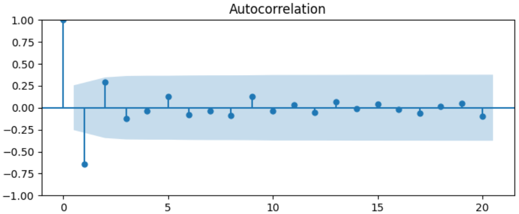
Figure 10.
Partial Autocorrelation: Periods in the time domain, remain within the 95% confidence interval.
Figure 10.
Partial Autocorrelation: Periods in the time domain, remain within the 95% confidence interval.
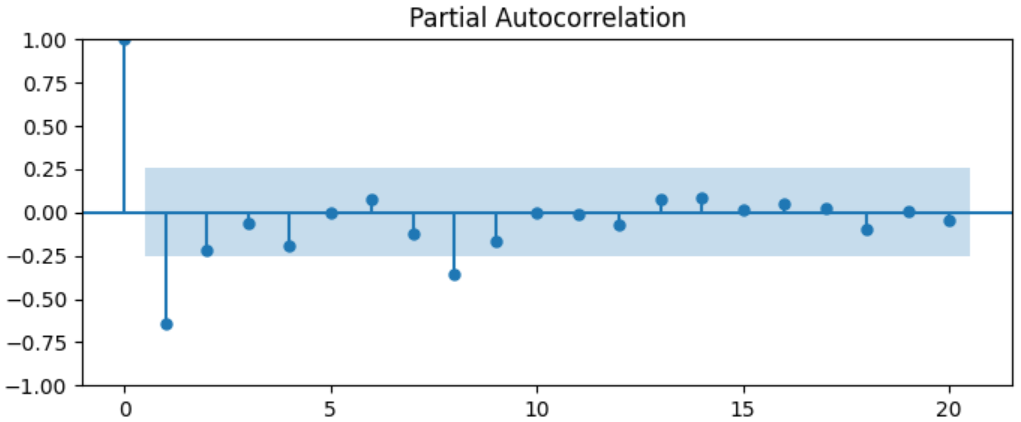
Figure 11.
Real data Consumption (2018-2022) and ARIMA forecast for 2023.
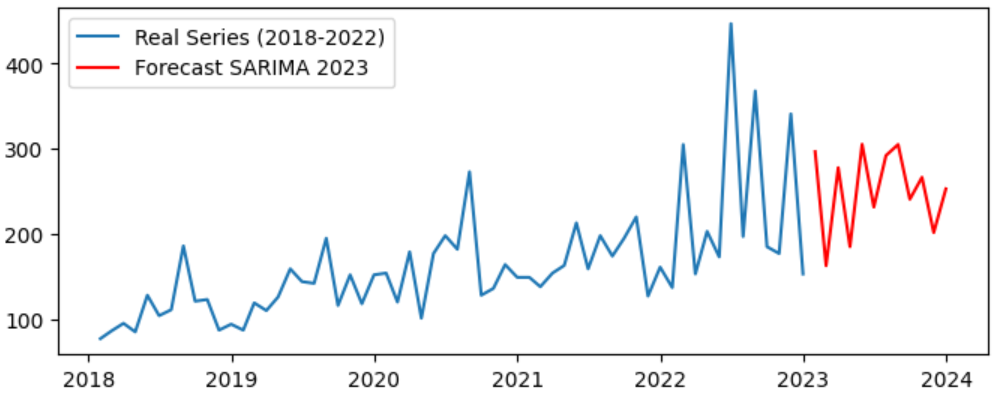
Figure 12.
Real data Consumption (2018-2022) and Holt-Winters forecast for 2023.
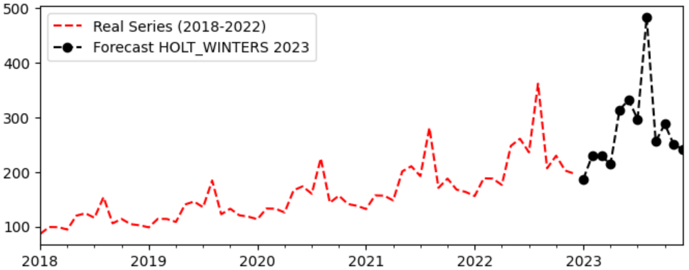
Figure 13.
Forecasts generated by ARIMA and Holt-Winters methods with the actual (2023) values observed.
Figure 13.
Forecasts generated by ARIMA and Holt-Winters methods with the actual (2023) values observed.
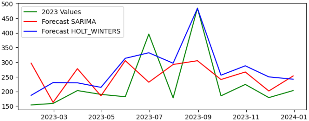
Figure 14.
Time Series 2018-2022 with forecasts (2023).
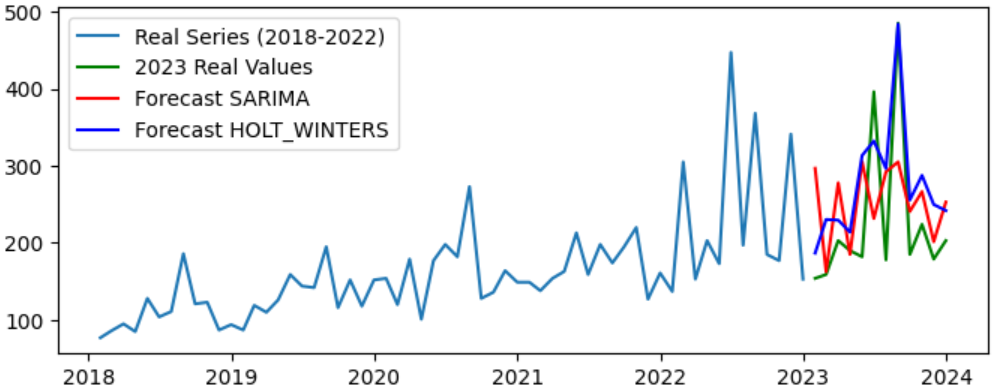
Figure 15.
MAE Evaluation: Comparison of the effectiveness of the forecasting methods (ARIMA and Holt-Winters).
Figure 15.
MAE Evaluation: Comparison of the effectiveness of the forecasting methods (ARIMA and Holt-Winters).
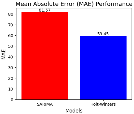
Figure 16.
MSE Evaluation: Comparison of the effectiveness of the forecasting methods (ARIMA and Holt-Winters).
Figure 16.
MSE Evaluation: Comparison of the effectiveness of the forecasting methods (ARIMA and Holt-Winters).
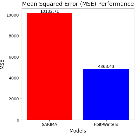

Table 1.
Cubic meters of water consumed monthly between 2018 and 2022.
| Year | Jan. | Feb. | Mar. | Apr. | May | Jun. | Jul. | Aug. | Sep. | Oct. | Nov. | Dec. |
| 2018 | 77 | 86 | 95 | 85 | 128 | 104 | 111 | 186 | 121 | 123 | 87 | 94 |
| 2019 | 87 | 119 | 110 | 126 | 159 | 144 | 142 | 195 | 116 | 152 | 118 | 152 |
| 2020 | 154 | 120 | 179 | 101 | 177 | 198 | 182 | 273 | 128 | 136 | 164 | 149 |
| 2021 | 149 | 138 | 154 | 163 | 213 | 159 | 198 | 174 | 195 | 220 | 127 | 161 |
| 2022 | 137 | 305 | 153 | 203 | 173 | 447 | 197 | 368 | 185 | 177 | 341 | 153 |
Table 2.
Comparison of Real Values and Forecasts from SARIMA and Holt-Winters Models.
| Date | Real Values | Forecast_SARIMA | Forecast_HOLT_WINTERS |
|---|---|---|---|
| 2023-01-31 | 154 | 297 | 187 |
| 2023-02-28 | 159 | 163 | 230 |
| 2023-03-31 | 203 | 278 | 230 |
| 2023-04-30 | 190 | 185 | 214 |
| 2023-05-31 | 182 | 305 | 313 |
| 2023-06-30 | 396 | 232 | 332 |
| 2023-07-31 | 178 | 292 | 296 |
| 2023-08-31 | 485 | 305 | 484 |
| 2023-09-30 | 185 | 241 | 256 |
| 2023-10-31 | 224 | 267 | 288 |
| 2023-11-30 | 179 | 202 | 250 |
| 2023-12-31 | 203 | 253 | 242 |
Disclaimer/Publisher’s Note: The statements, opinions and data contained in all publications are solely those of the individual author(s) and contributor(s) and not of MDPI and/or the editor(s). MDPI and/or the editor(s) disclaim responsibility for any injury to people or property resulting from any ideas, methods, instructions or products referred to in the content. |
© 2026 by the authors. Licensee MDPI, Basel, Switzerland. This article is an open access article distributed under the terms and conditions of the Creative Commons Attribution (CC BY) license (http://creativecommons.org/licenses/by/4.0/).
Copyright: This open access article is published under a Creative Commons CC BY 4.0 license, which permit the free download, distribution, and reuse, provided that the author and preprint are cited in any reuse.