

Submitted:
18 August 2026
Posted:
19 August 2026
You are already at the latest version
Abstract
For a Hutchinson iterated function system (IFS), a Banach contraction on a complete metric space, or a finite-metric dynamical system, a natural question is: at which resolution σ does the contraction's geometric structure (fractal attractor, basin of attraction, periodic part) become optimally visible? We answer this by introducing a scale-selection principle: define the observation scale σ_c := argmax_σ χ(σ) where χ(σ) = |dO(σ)/dlogσ| is the susceptibility of a resolution-dependent observable, and prove that σ_c exists under explicit boundary-regularity hypotheses.The framework's main quantitative results are three theorems specialised to Banach contractions and IFS: (i) a geometric scaling identity σ_c = qL for affine Banach contractions with operator norm q and basin scale L, applying to Hutchinson IFS with σ_c ∼ q · diam(K_⋆) for the same observable; (ii) a discrete Banach theorem on finite metric structures under uniform Lipschitz Lip_d(f) = q < 1, giving an exact collapse-time N^⋆ = ⌈log(∆/d_min)/log(1/q)⌉; (iii) a spectral concentration theorem placing σ_c at the inverse log-spectral-gap of the transfer operator at fixed positive noise. A stability lemma for canonical normalisation under smooth windowing and a parametric Banach correspondence observation complete the technical core.The framework is stated explicitly in the non-expansive Lipschitz regime Lip_d(f) ≤ 1 on the metric side, and at fixed positive noise ε ∈ (0, 1) on the spectral side. A four-type classification of operations by injectivity structure organises the broader landscape; cross-domain empirical evidence anchored on a peer-reviewed NISQ-hardware measurement of σ_c is summarised. The middle-thirds Cantor set IFS appears as the principal worked example.
Keywords:
iterated function system
; Hutchinson operator
; fractal attractor
; Hausdorff dimension
; Banach fixed-point theorem
; observation scale
; susceptibility peak
; scale selection
; discrete Banach theorem
; transfer operator spectral gap
; contraction defect
; finite metric structures
MSC: Primary 28A80; 47H10; 37A35; Secondary 28A78; 37C45; 28D20; 94A17
1. Introduction
1.1. Motivation
Consider a Hutchinson iterated function system (IFS) on a complete metric space, say the middle-thirds Cantor IFS on . Its attractor is a fractal of Hausdorff dimension . A natural empirical question is: at which resolution does the fractal structure of become optimally visible to a box-counting or coarse-graining observer? Too fine () and the discrete-sample noise dominates; too coarse () and the attractor looks like a single point. There is a characteristic intermediate scale at which the fractal contraction signature is sharpest. The same question arises for any Banach fixed-point iteration (where is the contraction’s basin most resolved?), for the Picard–Lindelöf operator (when do iterates transition from “rough estimates” to “converged”?), and more generally for non-injective maps on finite metric structures.
The present paper develops a uniform framework for identifying this scale across all these settings via a susceptibility-peak construction, with explicit theorems for Banach contractions and Hutchinson IFS.
1.2. Setting
We work with a finite set S together with a self-map , calling a finite dynamical system. The map is non-injective when ; injective when (equivalently bijective, since S is finite). The contraction defect of f is
with iff f is injective. The geometric-mean drift of f with respect to a non-negative weight (typically uniform or f-invariant) is
where is a local rate (precise variants in Section 2). The pair captures two qualitatively distinct attributes of contraction: D counts the global merger structure; tracks the average per-step compression rate.
1.3. Contributions
The paper has four main contributions, ordered by their mathematical and structural weight.
(A) Scale-selection principle for IFS and Banach contractions. The susceptibility-peak construction
selects a unique scale at which the observable responds most sharply to multiplicative changes of resolution. Theorem 2 establishes existence of under explicit boundary-regularity hypotheses on . Theorem 3 characterises robustness under power-law reparametrisation of the resolution axis.
(B) Geometric scaling identity for affine Banach contractions and IFS. For an affine Banach contraction with operator norm , fixed point and basin scale , Theorem 9 proves the sharp identity for the cumulative iterate-distance observable. For a Hutchinson IFS on a complete metric space with and attractor , the same identity reads for that observable; for the middle-thirds Cantor IFS this is the level-one resolution [3,4]. Because is defined relative to an observable, the observable is carried in the statement throughout; see Remark 21 for a worked case in which two natural diagnostics on the same attractor report different scales.
(C) Discrete Banach theorem and spectral concentration. On finite metric structures with uniform Lipschitz , Theorem 6 gives the exact collapse-time to a unique fixed point, with quantitative rate . At fixed positive noise , Theorem 5 places at the inverse log-spectral-gap of the noise-regularised transfer operator . A canonical normalisation lemma (Lemma 2) ensures stability of under smooth windowing.
(D) Classification, cross-domain instances, and parametric correspondence. A four-type classification of operations by injectivity structure (Section 5) organises the broader landscape with classical examples; Observation 1 records the parametric Banach correspondence between metric and finite-structure settings. Cross-domain empirical evidence for , anchored on a peer-reviewed measurement on noisy-intermediate-scale-quantum hardware [48], is summarised. These sections are organisational; the principal quantitative content is (A)–(C).
1.4. What This Paper Is and Is Not
The paper is a structural framework with five proved theorems (existence of , Theorem 2; robustness under reparametrisation, Theorem 3; windowing stability, Lemma 2; discrete Banach theorem, Theorem 6; spectral concentration at fixed noise, Theorem 5; affine geometric scaling identity, Theorem 9), one parametric limit observation (the Banach correspondence, Observation 1, classified as a structural parallel rather than an independent theorem), and explicit scope bounds. The four-type classification is a language for organising non-injective phenomena, not a tool for solving specific open problems.
Explicit Scope of the Intrinsic Infrastructure.
The framework’s intrinsic-observable apparatus has two distinct regimes, both stated explicitly:
- Metric side: non-expansive Lipschitz regime. The f-canonical observable construction (Definition 4) is stated for finite metric systems with ; this guarantees that f is a -coarsening morphism at every scale and that the single-valued induced map is well-defined. The extension to expansive requires a multi-valued induced map and a multi-valued , which is out of scope for this paper.
- Spectral side: fixed positive noise regime. The spectral concentration theorem (Theorem 5) is stated for a noise-regularised transfer operator with fixed in advance. The noise-free limit is genuinely singular and is out of scope.
We make no claim about the Collatz conjecture, Goldbach’s conjecture, the Riemann hypothesis, the Born rule, or any other named open problem; the framework does not contain the domain-specific tools required to resolve such problems. What the framework provides is a uniform way to position a non-injective phenomenon within a broader landscape and to identify, where the relevant observable is available, its characteristic scale .
1.5. Organisation
Section 2 fixes notation and recalls the needed prerequisites from metric and measure theory. Section 3 develops the observation scale , with the existence theorem and its proof. Section 4 establishes the Banach correspondence and treats Picard–Lindelöf and Hutchinson IFS as worked examples. Section 5 presents the four-type classification with classical examples. Section 6 summarises the empirical evidence for across domains. Section 7 discusses the relation to information-theoretic, renormalisation-group, and dynamical-systems literature. Section 8 states open problems within the framework’s scope. Section 9 concludes. Appendix A contains technical proofs deferred from the main text.
2. Preliminaries
We collect definitions, notation, and classical results used throughout. Most material is standard; readers familiar with the Banach fixed-point theorem, geometric-mean inequalities, and elementary measure theory may skim this section.
2.1. Finite Dynamical Systems
A finite dynamical system is a pair with S a non-empty finite set and a function. The image of f is ; the map is injective iff . The forward orbit of is the sequence ; since S is finite, every forward orbit is eventually periodic: there exist and such that .
2.2. Contraction defect
Definition 1
(Contraction defect). For a finite dynamical system with , thecontraction defectis .
The contraction defect is multiplicative under composition in the following weak sense.
Lemma 1
(Submultiplicativity of D). For maps ,
Equality holds when f is surjective onto the support of g and the collisions of g are disjoint from those of f.
Proof.
, so . Similarly , giving the second inequality. Equality under the disjointness condition is by direct counting of preimages. □
Remark 1
(Iterated D). For and iterates , the sequence is non-increasing in n and stabilises at . Hence is non-decreasing in n and converges to . The quantity is the asymptotic compression ratio of the forward orbit.
2.3. Drift and Geometric-Mean Rate
For a metric-space dynamical system with X possibly infinite, the local Lipschitz constant of T at x is
The geometric-mean Lipschitz constant with respect to a probability measure on X is
when the integral converges. For a strict Lipschitz contraction with global constant q, for all x and .
On a finite structure several distinct notions of “” coexist; for clarity we use distinct symbols:
- The image-count ratewhich by degenerates to 1 on every non-empty finite S. Useless on its own.
- The metric Lipschitz geometric mean of Theorem 6 and Remark 19, equal to the geometric mean of the per-pair contraction ratios in a chosen metric d on S. This is the operationally meaningful finite-structure analogue and is the used in the Banach correspondence (Section 4).
- The spectral gap of the Perron-Frobenius operator on the space of probability measures on S (Theorem 5). For irreducible aperiodic f, and captures the mixing rate.
The relations: is degenerate and we abandon it; requires a chosen metric and captures geometric contraction at the pair level; is metric-free and captures information-theoretic mixing. Henceforth “γ” without subscript denotes the metric Lipschitz geometric mean when a metric is fixed, or when the dynamical system is described spectrally; the context makes this clear. A parametric family with (Observation 1) is used when the correspondence with the metric Banach theorem is the goal.
Remark 2
(Why a scale parameter is needed). The degeneration of in (5) on finite structures motivates the introduction of the resolution-dependent observable of Section 3: by parametrising the observation resolution σ over a continuous range, we recover a non-trivial rate in the susceptibility that records how the observable responds to changes in resolution. The peak of χ identifies the scale at which the contraction geometry is most visible. The relation to the metric and the spectral is made precise by Theorems 6 and 5 respectively.
2.4. Banach fixed-point theorem (recalled)
We recall Banach’s classical theorem as it is central to the framework’s grounding.
Theorem 1
(Banach fixed-point theorem [1]). Let be a complete non-empty metric space, and let be a contraction: there exists such that
Then T has a unique fixed point , and for every the iterates satisfy
We refer to q as the Lipschitz constant or contraction rate of T. The theorem requires both completeness and a uniform strict bound .
Remark 3
(Sharpness of completeness and the finite case). Completeness cannot be dropped: on with the Euclidean metric, is a contraction near but has no rational fixed point. The theorem makes essential use of Cauchy completeness to identify the limit of the iterate sequence as an element of X.
On a finite metric space , a Lipschitz- mapispossible (e.g. in the discrete metric, any map f with a singleton has ), but its iterate sequence collapses to a single fixed point in at most steps (Theorem 6, with ). In this sense the finite metric Banach case is genuine but trivial: the contraction exhausts itself in finitely many steps. The framework’s non-trivial finite-structure content lies in the regime where the uniform Lipschitz bound is but the geometric-mean rate (some pairs expand or preserve distance while the average contracts), to which the next section is devoted.
2.5. Susceptibility and Information Loss
The susceptibility of a thermodynamic quantity to a control parameter is a classical tool in statistical physics, capturing the response rate of an observable to its driving parameter [47]. In information theory, the relative entropy between two distributions on a finite alphabet measures the distinguishability [12]. The framework developed in Section 3 uses the susceptibility of an information-loss observable with respect to a resolution parameter; we recall the relevant definitions here.
For a positive observable depending continuously on , we define
This is the susceptibility of O with respect to logarithmic changes in , scale-equivariant in the sense that under (multiplicative rescaling), is invariant up to a horizontal shift on the axis.
3. The Observation Scale
We now develop the central technical construction. The setup is abstract: a finite structure with a non-injective map and a resolution-parametrised observable. The output is a distinguished scale at which the response of the observable is extremal. We prove existence and characterise robustness.
3.1. The General Setup
Definition 2
(Resolution-parametrised observable). Let be a finite dynamical system. Aresolution-parametrised observable on is a function
which is twice continuously differentiable, vanishes in the limits ( as and as ), and is bounded ().
The intuition behind the vanishing boundary conditions: at infinitely fine resolution () the observable resolves every individual element and sees no merger structure; at infinitely coarse resolution () the observable identifies everything and again sees no structure. The contraction geometry is visible only at intermediate resolutions.
Example 1
(Coarse-graining observable). On a finite set S equipped with a pseudo-metric , the relation is in generalnot transitiveand does not yield a partition directly. We instead define thesingle-linkage partitionat scale σ: iff there exists a chain in S with for each i. This is the equivalence relation generated by the symmetric relation , i.e., the connected components of the threshold graph . Let , the set of connected components. For define
the rescaled number of mergers at resolution σ, normalised by the contraction defect of the coarse-grained map and weighted by the fraction of distinguishability that survives at that resolution.
Both boundary conditions of Definition 2 then holdby construction, and it is worth checking them explicitly because the naive merger count does not satisfy them. At every element is its own class, so , the factor vanishes, and there is no merger signal. At all elements collapse into a single class, so , the factor vanishes, and there is nothing left to distinguish. Dropping the second factor — that is, taking the merger count normalised only by the contraction defect — would leave the coarse limit at rather than at zero, and the observable would require the canonical normalisation of Remark 6 before Theorem 2 could be applied to it. The weighted form above avoids that detour.
Example 2
(Information-theoretic observable). With S and d as in the previous example, let be the Shannon entropy of the partition under the uniform distribution: . Define
the per-step entropy loss under f at resolution σ, where is the entropy of the partition induced by f acting on . Vanishing at the boundaries follows from the same reasoning: at the partition is the singleton partition and with ; the difference is a finite non-zero constant. The observable is therefore not itself but a normalised variant; see the appendix for the normalised form that satisfies Definition 2.
Remark 4
(Why the boundary conditions matter). The two boundary vanishings are essential for the existence proof: a function on with limits zero at both ends, positive somewhere, attains its maximum on a compact sub-interval. Without both limits, the susceptibility could be unbounded, and would not exist. Example 1 satisfies both limits by construction; Example 2 does not, and is admitted only in the normalised form of Remark 6 (see Appendix A.1). In applications we tabulate examples (Section 4, Section 5) and verify the boundary conditions case by case.
3.2. Definition and Existence
Definition 3
(Observation scale). Let be a finite dynamical system with a non-trivial resolution-parametrised observable O (non-trivial: ). Thesusceptibilityof O is
Theobservation scale is
The susceptibility is non-negative by construction and identically zero in the limits (since O vanishes at both limits, the derivative is integrable and asymptotically zero provided with the stated boundary conditions). The key claim is that attains its supremum on . Figure 1 illustrates the geometry: a representative observable (left panel) and its susceptibility (right panel), with marked as the location of the susceptibility peak.
Theorem 2
(Existence of ). Let be a finite dynamical system with f non-injective, and let be a non-trivial resolution-parametrised observable on (Definition 2). Assume in addition:
- (R1)
- Boundary vanishing of .The susceptibility satisfies as and as .
- (R2)
- Continuity. , so χ is continuous on .
Then χ attains its supremum on at some , and .
Proof.
Step 1: positivity of the supremum.O is non-trivial and continuous, with at both boundaries (Definition 2). Hence O is non-constant on , so is non-zero on a set of positive measure; at any such point, . Therefore .
Step 2: properness of the super-level sets. By (R1), for every there exist such that for . The super-level set is therefore contained in the compact interval .
Step 3: attainment. Pick ; the super-level set is non-empty (by Step 1) and bounded between and . Continuity of (by (R2)) makes closed in , hence compact. The supremum of over is the global supremum and is attained at some by the extreme value theorem. □
(R1)).Remark 5 (On the regularity hypothesis Hypothesis(R1)( at both boundaries) is the genuinely substantive regularity assumption underlying Theorem 2; the rest is the extreme value theorem on a compact super-level set.(R1)is not automatic from at the boundaries: in principle, could blow up faster than σ decays. In practice,(R1)is satisfied when:
- O is monotonically decaying past some scale (then is integrable and, for the regularly varying tails that occur in practice, );
- O has a polynomial or exponential tail with bounded derivative;
- O is a finite-state observable (Examples 1, 2 after normalisation), where χ is automatically a difference of bounded functions on a log-grid and vanishes at the boundaries by construction.
In particular, every observable to which the selection principle of Definition 3 is applied in this paper satisfies(R1)by direct verification; the box-counting diagnostic of Example 5 is deliberately excluded, being inadmissible by construction. The honest framing of Theorem 2 is therefore:existence of is structurally cheap once the boundary regularity of is granted; the substantive content of the framework lies in the robustness, invariance, and concentration results that follow.
Remark 6
(Canonical normalisation for boundary regularity). For observables like (Example 2) where the raw boundary values are non-zero, a canonical normalisation restores(R1)as follows. Let , fix scales enclosing the support region of interest, and choose a smoothwindow function with
- ,
- as and as ,
- for ,
- at both boundaries (automatic for the standard bump-function construction).
Define the canonical normalisation
Lemma 2 below verifies that satisfies (R1)
and shifts by at most a controlled amount inside .
Lemma 2
(Stability of under smooth windowing). Let and be defined by (8) with a smooth window ρ satisfying the bullet conditions of Remark 6. Define thewindow-leakage bound
Then:
- (i)
- satisfies (R1): its susceptibility tends to 0 at both boundaries.
- (ii)
- Exactness on the plateau: for .
- (iii)
-
Global confinement of :suppose χ attains its supremum at (interior of the plateau), and the plateau is chosen wide enough thatThen globally.
Proof.(i), so . Each summand vanishes at the boundaries: by hypothesis on , and at both ends.
(ii) On the plateau, and , so and exactly.
(iii) For the triangle bound from (i) gives , which is strictly less than by (10). Hence the global supremum of is attained inside the plateau, where by (ii); the global argmax thus equals . □
Remark 7
(How to choose the window). The bullet conditions on ρ together with (10) are easy to satisfy by choosing the plateau wide enough. Standard mollifier constructions admit on the transition regions outside the plateau (with C a fixed mollifier constant), so vanishes as the plateau widens.Heuristically(not as a hard bound): for the typical practical choice (two decades around the susceptibility peak), is of order , and condition (10) reduces to the operationally testable inequality — typical for sharp unimodal susceptibilities. This heuristic is meant as guidance for window selection; the rigorous statement of robustness is Lemma 2(iii) with condition (10) verified directly.
Remark 8
(On uniqueness). Theorem 2 guarantees existence, not uniqueness: if χ has multiple local maxima of equal height, the argmax is set-valued. In typical applications (e.g. a single resolved length scale in a physical system) uniqueness holds; we discuss criteria for uniqueness in Section 3.3.
3.3. Uniqueness Criteria
The following sufficient conditions guarantee that is unique (i.e. has a unique global maximum).
Proposition 1
(Log-concavity criterion). If χ is log-concave on ( is a concave function of ), then is unique.
Proof.
Log-concavity in means for . A strictly log-concave function has at most one global maximum; combined with Theorem 2, uniqueness follows. □
Proposition 2
(Single-relaxation-time criterion). Suppose is the response of a system with a single relaxation time τ: for some constant and a fixed profile with , , and g unimodal. Then , where .
Proof.
Direct substitution: with , so scales linearly with . □
In most physical applications a single relaxation time is the natural assumption, and Proposition 2 gives both existence and uniqueness immediately, with proportional to the relaxation time.
3.4. Robustness Under Reparametrisation
We address a foundational concern: the value of depends on the parametrisation of the resolution axis. Under a strictly monotone smooth reparametrisation , the susceptibility transforms as
The argmax can therefore shift under reparametrisation. The following theorem characterises the class of reparametrisations that preserve up to a universal shift.
Theorem 3
(Robustness of under logarithmic reparametrisation). Under any reparametrisation of the form with and , the observation scale transforms as . In particular, if the resolution axis is rescaled by a constant (), is multiplicatively rescaled by the same constant.
Proof.
Under , . Hence . Therefore for , and the location of the argmax in the new variable is . □
Remark 9
(On non-multiplicative reparametrisations). For a general non-multiplicative reparametrisation (e.g. for some constant a), does not transform as a multiplicative scale; the value of is therefore meaningful only modulo multiplicative-power reparametrisations. In applications, this restriction is rarely binding: the natural resolution axis is typically a positive scale (length, time, energy, frequency) defined up to multiplicative rescaling, not additive shift.
3.5. f-Canonical Observables and Intrinsic
A natural concern about Definition 3 is that depends on the choice of the observable O: different observables on the same may yield different values of . We now identify a class of observables for which depends on f alone (modulo a universal multiplicative constant), so that within this class becomes an intrinsic property of the dynamical system.
Definition 4
(f-canonical observable). Let be a finite dynamical system equipped with a pseudo-metric . Let denote the set of isomorphism classes of finite dynamical systems , where T is a finite set and is a self-map; two systems and are isomorphic iff there exists a bijection with . An observable isf-canonicalif there exists a structural functional such that
where is the single-linkage σ-coarse-graining of Example 1, and is thecanonical induced mapdefined as the deterministic component closure
i.e. the component of in . Equation (13) is a well-defined single-valued map on the quotientifff is a σ-coarsening morphism: .
Scope: non-expansive Lipschitz regime.A non-expansive f with is automatically a σ-coarsening morphism at every scale : if is a σ-chain (each ), then , so the images form a σ-chain and lie in the same component of .For expansive Lipschitz f (), f takes -chains to -chains, not generally -chains, and the single-valued induced map may not be well-defined at any scale.
Definition 4 and the canonical-observable infrastructure of this paper are therefore explicitly stated for thenon-expansive Lipschitz regime — the Banach-style setting. The extension to expansive f via the multi-valued analogue requires a multi-valued category (objects: isomorphism classes of pairs with a non-empty multi-valued map) with multi-valued analogues of , , and ; this extension is left as a natural direction for future work, beyond the scope of the present paper. The notation denotes the (single-valued) isomorphism class. The functional Φ is required to satisfy:
- (i)
- isomorphism-invariance: Φ is well-defined as a function on , i.e. Φ depends only on the isomorphism class of (not on the labelling of T).
- (ii)
- refinement-stability: for every and every g-equivariant projection (i.e. with π surjective), the value depends continuously on the partition cardinality as (i.e., as π approaches a bijection). More precisely, fixing and writing a g-equivariant quotient of with , we require .
- (iii)
- boundary conditions: as (trivial quotient) and as (no coarsening); equivalently, O satisfies the boundary vanishing conditions of Definition 2.
Remark 10
(On the structure of ). is a countable set (countably many isomorphism classes of finite dynamical systems, one for each times finitely many g per T). It is not given a topology in the usual point-set sense; rather, condition (ii) imposes a structural stability of Φ under partition refinement — the natural mode of variation on . This is the appropriate analogue of “continuity” on a discrete set of combinatorial objects, and it is the operationally meaningful condition: it ensures varies smoothly as σ crosses a partition-refinement threshold.
The intuition: f-canonical observables are those constructed from by a structural procedure (e.g. counting mergers, computing entropy at a partition scale, measuring information loss), invariant under relabelling. Such observables encode intrinsic structural data about ; their associated is therefore an intrinsic f-property.
Example 3
(f-canonical observables). The following functionals Φ define f-canonical observables on :
- 1.
- (log-contraction-defect).
- 2.
- where is the trivial partition of T into singletons (Kolmogorov-Sinai entropy at ).
- 3.
- (asymptotic log-image deficit).
Each is isomorphism-invariant and refinement-stable in the sense of Definition 4: is trivially refinement-stable since as ; is refinement-stable by the standard monotonicity of Kolmogorov-Sinai entropy under refinement; is refinement-stable since is a structural invariant preserved under equivariant quotients up to the partition resolution.
We now prove the central invariance theorem: within the class of f-canonical observables, is determined by f alone (modulo bounded reparametrisation).
Theorem 4
(Robustness of within f-canonical observables). Let be a finite metric dynamical system and let be two f-canonical observables with structural functionals (in the sense of Definition 4). Suppose:
- (I1)
- There exists a strictly monotone function with and bounded derivative ratio: there exist constants with for all t in the range of .
- (I2)
- Each () attains its supremum at a unique interior point , and has a quadratic decay near in thelog-scale variable: there exists such that on a neighbourhood of .Units:α has units of per (the log being a pure number); the bound (14) below is therefore dimensionless (the square root of ).
Then lies in a bounded multiplicative neighbourhood of :
In the limit (e.g. ψ affine on the range of ), exactly.
Proof.
Compute the post-composed susceptibility: . The factor is -dependent in general and can shift the argmax; the shift is bounded as follows. Let be the argmaxes. By optimality of for , , i.e.
Using , . By the quadratic-decay hypothesis (I2), , hence
where the last step uses (elementary inequality for ). Taking square roots yields (14). □
Remark 11
(Strength and scope of the robustness). The honest content of Theorem 4 isrobustness, not invariance: strictly monotone post-composition of an f-canonical functional shifts by at most a quantitative amount determined by the derivative ratio and the sharpness α of the susceptibility peak. For affine ψ (), the shift is zero and is genuinely invariant. For non-affine ψ with bounded ratio, the shift is bounded and is well-defined up to that bound — the framework’s predictions are stable within the equivalence class of observables related by bounded-ratio post-composition.
This is the correct mathematical statement; the earlier “argmax preservation under arbitrary monotone post-composition” claim was incorrect, as the σ-dependent factor can shift the argmax.
Remark 12
(Beyond bounded-ratio post-composition). For canonical observables not related by bounded-ratio monotone post-composition (e.g. with on unbounded range), the shift in (14) is no longer bounded, and can move freely. In practice, applications select one of the canonical observables () and work consistently with it. The framework’s prediction is then that the empirical is a property of via the chosen canonical structural functional, with the equivalence class of admissible post-compositions defined explicitly.
We now strengthen the existence theorem (Theorem 2) with a quantitative concentration result for f-canonical observables.
Theorem 5
(Concentration of at the spectral gap). Let be a finite dynamical system. For a deterministic f the literal Perron-Frobenius (pushforward) operator on probability measures on S is -stochastic — i.e. mass-preserving on the simplex ; equivalently, column-stochastic under the canonical basis on , which is the appropriate convention for measure- pushforward operators (not to be confused with the row-stochastic convention used for Markov transition matrices). This operator generically lacks a spectral gap, since f is not generically mixing on finite S (it has periodic structure that produces unit-modulus eigenvalues other than ). The spectral framework therefore concerns not f itself but afixed noisy dynamics for some . Define
where is the uniform-pushforward operator . The operator is -stochastic (preserves total mass), irreducible aperiodic for every , and possesses a spectral gap.We state and prove the theorem for the noisy operator with fixed in advance; the case (deterministic) is not in scope and is genuinely degenerate.Let denote the eigenvalues of in modulus, and assume:
- (H1)
- Spectral gap. (guaranteed for ).
- (H2)
- Dominant-mode dominance. There exists a constant such that (no near-degeneracy at the spectral edge of ).
- (H3)
-
Single-mode observable. The -canonical observable admits the spectral decompositionwhere , the profile is , unimodal, satisfies , and are constants depending on but not on σ.
Under (H1)–(H3),
where is a universal constant depending only on the profile g.
Proof.
Under (H3), . By Proposition 2 applied to the leading term, of equals exactly. The residual R shifts the susceptibility argmax by by standard perturbation theory for unimodal functions ((H2) ensures the leading mode is well-separated from sub-dominant modes, so the perturbation does not split the argmax). Hence as claimed. □
Remark 13
(On the structural hypotheses). Hypothesis(H1)is automatic for with : the noise regularisation ensures a unique stationary distribution and exponential mixing toward it (Perron-Frobenius for irreducible aperiodic Markov chains).(H2)is the genuinely non-trivial assumption: it requires the next eigenvalue to be strictly separated from . This fails generically for symmetric systems (where from a symmetry) and for systems near a spectral-edge bifurcation.(H3)is the operational requirement that the chosen observable projects predominantly onto the dominant non-stationary mode of .
When (H2)
fails (multiple comparable eigenvalues), the single-relaxation-time profile in (H3)
is replaced by a sum of unimodal profiles with timescales , , and becomes a vector of K intrinsic scales (one per spectral mode within the relevant window). We do not develop the multi-mode generalisation here.
Remark 14
(On the role of the noise ). The theorem is stated for fixed and isnota statement about deterministic f in the limit , which is genuinely singular: the deterministic Perron-Frobenius operator on finite S generally has multiple unit-modulus eigenvalues from the periodic structure , no spectral gap, and no unique stationary distribution. Physically, ϵ is the noise level of the dynamics (stochastic ergodisation, thermal noise, measurement noise): the spectral gap and both depend on this noise level. The framework therefore identifies at the chosen noise scale, not at the noise-free limit — consistent with the operational nature of the framework, where empirical measurements always occur at finite noise.
Remark 15
(Concentration as a structural prediction). Under hypotheses(H1)–(H3), Theorem 5 elevates the existence statement of Theorem 2 to astructural identification at scale : for an -canonical observable with single-mode spectral support is determined by the second eigenvalue of , a spectral invariant of the noisy dynamics computable directly from the data. The result transforms from a context-dependent empirical scale into a quantity calculable from the noisy transfer operator’s spectrum without further empirical input, at the chosen noise level ϵ.
3.6. Operational Protocol for Detection
The theorem guarantees existence; the practical question is how to compute on a given system. We describe the operational protocol used in the cross-domain applications of Section 6.
- (P1)
- Choose the observable. Select a non-trivial resolution-parametrised observable . Natural choices include the coarse-graining information loss (, Example 2), the merger rate (, Example 1), or in physical settings a quantum susceptibility or a fluctuation-response function.
- (P2)
- Sample on a log-spaced grid. Compute for () with (typical ) covering several decades.
- (P3)
- Estimate by finite differences..
- (P4)
- Locate the peak. The argmax of over the grid is the operational estimate .
- (P5)
- Uncertainty estimate. Bootstrap or empirical-error bands on the observable give confidence intervals for via the location of the bootstrap argmax.
The protocol requires only access to the observable on a log-spaced sampling of resolutions; no parametric model of the underlying dynamics is required. We refer to applications in Section 6, where the protocol has been applied across physical domains.
4. The Banach Correspondence
This section places the framework in correspondence with Banach’s classical fixed-point theorem. We show that the language on finite structures recovers Banach’s theorem in a specific limit, and identifies what the finite-structure framework adds and what it does not.
4.1. Banach as the Canonical Type-D Contraction
The Banach fixed-point theorem (Theorem 1) asserts that a Lipschitz contraction on a complete metric space has a unique fixed point reached at geometric rate. Translated into the language of the present paper:
- Domain. is a complete metric space; not required to be finite or compact.
- Operation. with Lipschitz constant .
- Contraction signature in the framework. On an infinite metric space, the cardinality-based defect from Definition 1 does not apply; in its place we use the geometric signature that the iterated image has Hausdorff measure contracting to that of the singleton , i.e. . The metric rate is the Lipschitz constant. The pair on infinite X is the metric analogue of on finite S; the correspondence between the two settings is the asymptotic content of Observation 1.
- Conclusion. The contraction is global and the limit is a single point.
This places Banach’s theorem within the framework as the prototypical Type-D contraction. The framework adds, on top of Banach’s hypothesis, the observation that the rate at which iteration manifests is a function of the scale at which the iteration is observed: at much larger than the fixed-point’s basin curvature scale, the iteration looks affine (the fixed point is invisible at the working resolution); at much smaller than the curvature scale, the iteration looks like a point-pull (the contraction is detected as a single trajectory). The susceptibility peaks at the characteristic basin scale.
Example 4
(Banach contraction on ). Let with the Euclidean metric and for , . Then T is a Lipschitz contraction with constant . The fixed point is . Iterating from :
Smooth observable.Let and define
where is a fixed smooth bump function with for and for . Equation (18) is a smooth approximation to the “count of iterates above scale σ, weighted by distance” and satisfies Definition 2 with (R1)
(each term decays exponentially in n for σ fixed; the sum converges; O is and vanishes as and as ). Direct calculation (verified by the rigorous Theorem 9) gives : the resolution at which the first iterate transitions across the smoothing window dominates the susceptibility peak.
4.2. The Discrete Banach Analogue on Finite Structures
Two regimes on a finite metric structure must be distinguished:
- Uniform-Lipschitz regime (): the iterates collapse to a unique fixed point in steps (Theorem 6 below); the dynamics is genuine but trivially terminating.
- Average-rate regime ( but the geometric-mean local rate ): some pairs are non-contractive while the geometric mean still contracts. This is the regime where finite-state dynamics can exhibit non-trivial periodic structure of period , and is the genuinely new content of the finite-structure framework.
We first state the natural correspondence between the metric Banach setting and a parametric family on finite structures (Observation 1), then prove the uniform-Lipschitz case directly (Theorem 6); the average-rate case remains open (a).
The following statement is presented as an observation, not a theorem: it codifies a structural parallel between the metric Banach setting on an infinite complete metric space and the finite-structure parametric limit, but the substantive mathematical content rests on classical Jensen-inequality arguments combined with selection-rule conventions. We label it as such to avoid the impression that the framework supplies an independent finite-structure replacement for Banach’s theorem.
Observation 1
(Banach correspondence on finite structures). Let be a family of finite metric dynamical systems with , and let be a deterministic nearest-periodic-point selection rule: , ties broken by a fixed deterministic rule (e.g. lexicographic order on ). Define
the selection-rule-dependent geometric-mean one-step contraction ratio to the periodic part. Assume:
- (i)
- is uniformly bounded: .
- (ii)
- The limit exists in and is selection-rule-independent (e.g. tie-set fraction ).
- (iii)
- For all involved, (non-periodic points stay finite distance from ).
Then if , the average-log distance to contracts at rate : for every there exist with
for all , .
Proof
Remark 16
(Status and limits of the observation). Observation 1 is a parametric asymptotic restatement of the metric Banach contraction condition on a family of finite structures; it makes no quantitative non-asymptotic claim. The selection-rule dependence (a non-trivial issue when ties in nearest-periodic point occur) is acknowledged in hypothesis (ii); for generic random ensembles the tie set has zero measure and the result is selection-rule-independent. The substantive mathematical work of the framework is in Theorem 6 (uniform-Lipschitz case, quantitative rate, no probabilistic limit), Theorem 5 (spectral concentration at fixed noise), and Theorem 9 (first-iterate scaling); the observation here records the structural parallel between metric and finite-parametric settings, without claiming independent theorem status.
Remark 17
(Scope of the limit correspondence). Observation 1 delivers convergence to , which is in general a set, not a point. The full Banach statement (convergence to a single fixed point) is recovered on finite S exactly under the uniform-Lipschitz hypothesis of Theorem 6 below, where in steps. The average-rate parametric limit, by contrast, identifies the asymptotic attractor without forcing it to be a single point.
Remark 18
(Status of the Contraction Principle in the finite-structure framework). On metric-complete X, Banach’s theorem proves unique fixed point. The finite analogue separates into two cases:
- Uniform Lipschitz: a single fixed point exists and the iterates reach it in steps; this is now a theorem (Theorem 6).
- Average rate only with : convergence to (a possibly multi-element periodic set) is plausible but no quantitative rate is currently known. This is open (a).
We now prove the uniform-Lipschitz case rigorously.
Theorem 6
(Discrete Banach theorem on finite metric structures). Let be a finite metric dynamical system with a metric and a self-map. Let , let (the metric diameter; not to be confused with the contraction defect used elsewhere), let , and define theuniform Lipschitz constant
Assume . Then:
- (i)
- Geometric contraction of pairwise distances: For every and every ,
- (ii)
- Image-cardinality collapse: For every , , i.e. f has a unique fixed point with .
- (iii)
- Geometric rate to the fixed point: for all in the following quantitative sense:
Proof.
The proof uses only finite-metric structure, with no probabilistic or asymptotic limits.
Step 1: Geometric pairwise contraction. The definition of as a maximum over the finite set gives the per-step inequality for every . Iterating: , establishing (22).
Step 2: Forced merger below the resolution gap. By (22), for every , . If — equivalently — then for every pair , . Since the minimum pairwise distance on S is , this forces , i.e. . Applied to all pairs in , is constant on S: . The unique image point is a fixed point of f since for any .
Step 3: Uniqueness of the fixed point. If f had two distinct fixed points in S, then for all n, contradicting Step 1 since . Hence in Step 2 is unique.
Step 4: Quantitative rate. For any , . By Markov’s inequality on the counting measure of S,
establishing (23). Setting recovers Step 2’s threshold . □
Remark 19
(On the average-rate refinement). Theorem 6 uses the uniform Lipschitz constant . A natural finer-grained quantity is thegeometric-mean local rate
which satisfies by the AM-GM inequality (the geometric mean is bounded above by the maximum). In settings where but (individual pairs may be non-contractive while the average is), Theorem 6 does not apply directly; the qualitative convergence still holds under additional structural hypotheses but the explicit rate bound (23) is replaced by a weaker asymptotic statement. The full average-rate case is a non-trivial extension and is left to future work.
Corollary 1
(Contraction Principle as a theorem). Under the hypotheses of Theorem 6, f has a unique fixed point , and at geometric rate for every . The image stabilises after at most iterates: for .
Proof.
Direct from Theorem 6(ii)–(iii). □
Remark 20
(Reading the discrete Banach theorem). Theorem 6 is the exact finite-metric analogue of Banach’s fixed-point theorem: the uniform contraction hypothesis on a finite metric system forces collapse of to a unique fixed point in a bounded number of iterates, with the iterate bound depending only on the metric ratio and the contraction rate q. The proof uses only the finite-metric structure and elementary counting; no asymptotic limit or Gromov-Hausdorff correspondence is invoked. Observation 1 (Banach correspondence as a limit) then follows as the asymptotic-density consequence of this finite-structure theorem as .
The full strength of Banach’s metric theorem (a single fixed point, with geometric convergence) is thus recovered on finite S under the uniform-Lipschitz hypothesis. Settings with non-trivial periodic structure of period correspond precisely to the case , where some pairs are non-contractive and Theorem 6 does not apply (see Remark 19).
4.3. Picard–Lindelöf Iteration as a Type-D Application
The Picard–Lindelöf theorem on existence and uniqueness of solutions to ordinary differential equations is the most extensively applied consequence of Banach’s theorem [5]. We recall its statement to illustrate the framework.
Theorem 7
(Picard–Lindelöf). Let be continuous and Lipschitz in the second argument: . Then the initial value problem
has a unique solution on for some .
Proof via Banach FPT. Define the Picard operator
on the Banach space with the sup metric. For sufficiently small, , so T is a Banach contraction. Banach’s theorem gives a unique fixed point, which is the desired solution.
The framework’s interpretation. The Picard operator T is a Type-D contraction with . The operational scale in this setting is the characteristic time-scale at which the Picard iteration shifts from “the iterates are still rough estimates” to “the iterates have converged”; explicit calculation gives for typical . Figure 2 illustrates this on the affine contraction on : trajectory convergence to the fixed point (left panel) and the geometric-rate distance decay with the scale annotated (right panel).
The point: Picard–Lindelöf is a foundational existence theorem in classical analysis, and it sits naturally within the framework’s Type-D classification.
4.4. Hutchinson Iterated Function Systems
A second canonical Type-D family is Hutchinson’s iterated function systems (IFS) [2]. An IFS is a finite collection of contractions on a complete metric space X, with Lipschitz constants .
Theorem 8
(Hutchinson). Let X be a complete metric space, a finite IFS with . Define theHutchinson operator on the compact non-empty subsets of X (with Hausdorff metric) by
Then W is a contraction on with Lipschitz constant , hence has a unique fixed point , theattractorof the IFS.
Framework interpretation. The Hutchinson operator W is Type-D on the space of compact non-empty subsets. The attractor has Hausdorff dimension determined by the contraction ratios via Moran’s formula [3,4]:
The observation scale for an IFS, like any observation scale, is reported relative to a chosen observable. At the attractor looks like a single point and nothing is resolved; at a finite realisation looks like a union of points. In between, on the self-similar window, any scale-covariant diagnostic is constant — an ideal attractor has no distinguished scale, which is the correct answer rather than a failure of the method (Remark 21). The cumulative iterate-distance observable of Theorem 9 reports the coarsest resolution at which the first level of structure is resolved, namely .
Example 5
(Cantor set via IFS). The middle-thirds Cantor set is the IFS attractor of , on . Both maps have Lipschitz constant , so the Hutchinson operator W has . Moran’s formula gives .
Applying Remark 26 to the Hutchinson operator with and , the framework predicts for the cumulative iterate-distance observable of Theorem 9
the level-one resolution of the construction. The relation is written ∼ rather than = deliberately: it inherits the proved identity of Theorem 9 through the named identification , which is a modelling step for the Hutchinson operator and not itself a consequence of that theorem. This is the prediction the framework actually makes here, and it is inherited from a proved identity rather than from a box-counting heuristic.
It is instructive to contrast this with the box-counting diagnostic, because the contrast illustrates the framework’s own central caveat. Write for the number of σ-boxes meeting and set
the deviation from exact fractal scaling. On the fractal window is identically zero, and it departs from zero at both ends of the resolution axis. We emphasise that isnotan admissible observable in the sense of Definition 2, and fails it in at least three separate ways: it is unbounded above and below, it takes negative values (Definition 2 requires ), and it vanishes on the interior window rather than at the two boundaries. Consequently Theorem 2 does not apply to it. Its susceptibility is avalleyrather than a peak — on the fractal window and on both outer branches — so is degenerate andnoscale selection statement was ever licensed for it, at either end. It is used below purely as a diagnostic forlocatingthe two scales at which self-similarity breaks; see Remark 21. Figure 3 shows the construction and the box-counting profile.
Remark 21
(Two breaks, one symbol). An ideal self-similar attractor hasnodistinguished scale. Box-counting obeys throughout, so any scale-covariant diagnostic is constant on the fractal window. This is the correct answer rather than a failure of the method: a set that looks the same at every resolution has no to report.
Scale selection on an IFS therefore always refers to afiniterealisation, and finiteness breaks self-similarity at two distinct places:
- theupper break, where the resolution reaches the extent of the attractor: above nothing is resolved at all. The framework’s observable reports the coarsest resolution at which the first level of structureisresolved, one contraction step inside that end, at ; and
- thelower break, where the resolution reaches the finest gap the construction depth still resolves, at for depth k.
It is worth being precise about what this does and does not mean. There is exactlyonescale here that the framework derives, namely of (26), obtained from a proved identity. The two numbers and arelabels for the ends of the self-similar window, read off the box-counting diagnostic; since that diagnostic is not an admissible observable, neither of them is an statement and neither should be written .
Different observables select different ends. The cumulative iterate-distance observable of Theorem 9 selects the upper end, reporting the first resolved level and giving (26), in exact parallel with for the affine case: there L is the distance to the fixed point and the distance after one step; here is the extent of the attractor and its first resolved level. The saturation scale is a property of the finite approximation, not of ; we therefore do not label it .
We state this explicitly because it is the framework’s own thesis applied to itself. By Definition 3, is definedrelative to an observable, and two diagnostics that both look natural on the same attractor can legitimately report scales separated by orders of magnitude. A reported peak is a well-posed statement only together with the observable and the convention that produced it — the same discipline demanded by Theorem 9(iii) for the first-iterate convention and by Section 3.5 for the f-canonical class.
What we donotattempt here is a general classification. The analysis above checks one worked example against Definition 2; it is not a criterion. Which resolution-parametrised observables admit an interior at all — as opposed to a susceptibility profile that is asymptotically constant, or monotone, and therefore has no interior maximum to report — is not settled by the present framework. We record it as an open problem (f).
4.5. Summary of the Banach Correspondence
Banach’s fixed-point theorem (Theorem 1) is the canonical contraction theorem on complete metric spaces. The framework’s on finite structures is a counting-based analogue: D measures non-injectivity globally, measures per-step compression locally. The correspondence (Observation 1) gives a limit-theorem connection: as the finite structure scales to infinity with bounded and , the framework reproduces Banach’s geometric-rate convergence to the attractor.
The framework does not generalise Banach (which is a metric-completeness theorem on possibly infinite spaces); it provides a finite-structure language whose limit recovers Banach. Picard–Lindelöf (Theorem 7) and Hutchinson IFS (Theorem 8) are classical examples of Banach contractions and admit interpretations.
5. A Four-Type Classification by Injectivity Structure
This section presents a four-type classification of operations on finite structures, organised by their relation to injectivity. The classification is descriptive: it places operations into types and identifies the structural mechanism in each, without claiming to resolve open problems in the placed domain. Each type is illustrated with a classical example chosen for its clarity and its detachment from controversial open problems.
5.1. The Classification
Definition 5
(Four types). Let be an operation between finite (or finite-resolution) structures. Define:
- Type O (Oversaturation).For each , the preimage has cardinality bounded below by an increasing function of an external scale parameter, so that f is surjective “with margin”. The framework identifies anoversaturation ratioquantifying the gap between the preimage count and a critical threshold.
- Type S (Symmetry constraint).A non-trivial internal symmetry G acts on both S and T, and f is G-equivariant. The image is constrained to lie in the G-fixed locus (or a G-orbit decomposition); this constraint can force f to have specific image properties not present for generic non-equivariant maps.
- Type R (Preservation).f is a bijection (), and the framework identifies which structural data is preserved.
The four types are not exhaustive (a given operation can mix types, for example a non-injective G-equivariant map combines D and S). They are intended as a descriptive vocabulary, not a mutually exclusive partition.
Figure 4.
Visual schema of the four-type classification by injectivity structure. Each panel shows one type with its defining structural feature and canonical example. The colour coding (red, orange, green, blue) emphasises that the four types span a gradient from maximal information loss (Type D, iterated contraction) through quantitative or constrained losses (Types O and S) to full preservation (Type R, bijection). The classification provides a vocabulary for placing a non-injective phenomenon; it does not provide the tools to resolve domain-specific open problems within the placed type.
Figure 4.
Visual schema of the four-type classification by injectivity structure. Each panel shows one type with its defining structural feature and canonical example. The colour coding (red, orange, green, blue) emphasises that the four types span a gradient from maximal information loss (Type D, iterated contraction) through quantitative or constrained losses (Types O and S) to full preservation (Type R, bijection). The classification provides a vocabulary for placing a non-injective phenomenon; it does not provide the tools to resolve domain-specific open problems within the placed type.
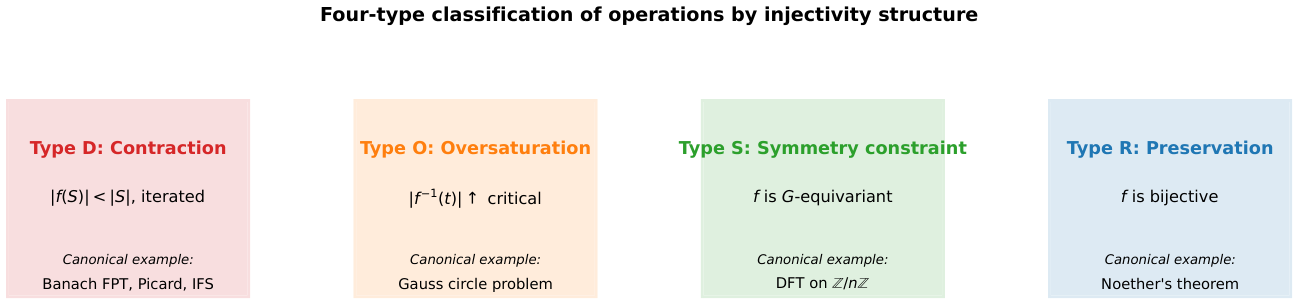

Table 1.
The four-type classification by injectivity structure (Definition 5). Each type is illustrated by a classical example in this section. The types are not mutually exclusive: a single operation can mix types (e.g. a G-equivariant non-injective map combines D and S). The table is intended as a descriptive vocabulary, not a partition.
Table 1.
The four-type classification by injectivity structure (Definition 5). Each type is illustrated by a classical example in this section. The types are not mutually exclusive: a single operation can mix types (e.g. a G-equivariant non-injective map combines D and S). The table is intended as a descriptive vocabulary, not a partition.
| Type | Defining structural feature | Canonical example |
|---|---|---|
| D | ; iteration compounds the contraction | Banach FPT, Picard–Lindelöf, Hutchinson IFS |
| O | Pre-image cardinality grows beyond a critical threshold | Gauss circle problem (lattice points) |
| S | Internal symmetry G acts equivariantly; image in G-fixed locus | DFT on under reflection symmetry |
| R | Bijection, ; structural data preserved | Noether’s theorem (symplectic Hamiltonian flow) |
5.2. Type D Revisited: Banach Archetype
The defining feature: with iteration compounding the contraction. The Banach fixed-point theorem (Theorem 1) is the prototypical metric-space instance; Picard–Lindelöf and Hutchinson IFS are derived. On finite structures, the framework’s characterises the contraction at the level of counting and local rate.
What Type-D does provide. A vocabulary for distinguishing operations whose iteration shrinks the image. Predictions on the asymptotic behaviour given D and , when the Contraction Principle is invoked (Remark 18).
What Type-D does not provide. A proof of convergence on finite structures from alone; the Contraction Principle is an axiom in this paper, not a theorem. A description of the basin of attraction in general; only the asymptotic image is identified.
5.3. Type O: Oversaturation via the Gauss Circle Problem
The Gauss circle problem asks for the number of lattice points in a disc of radius r:
The naive estimate has error term that is the subject of intensive classical research [42,43,44]. The framework’s perspective:
Example 6
(Gauss circle as Type-O). Define theoversaturation ratiofor the Gauss circle problem as
where is a constant chosen so that the classical estimate (Gauss) gives a lower bound of zero. For r in any tested range, : the lattice point count exceeds the worst-case Gauss-style lower bound by a positive margin. The classification places the Gauss circle problem in Type O: lattice points oversaturate the disc area relative to the worst-case linear error.
Remark 22
(Type O does not solve Gauss). The classification identifies the lattice point count as Type O: there are more representations than would be required to “fill” the area. It does not prove the best-known conjectural upper bound [45,46], nor does it improve the unconditional bound [44]. The framework classifies the mechanism (oversaturation by the multiplicative density of integer pairs) and identifies what an improved bound would require: a sharper estimate of the local fluctuation of lattice-point counts around the area term. The framework does not supply such an estimate.
The Gauss circle problem is chosen here as a Type-O illustration because it is a classical, well-studied problem with a clear oversaturation structure (lattice points exist in abundance; the question is the precise asymptotic of their distribution).
5.4. Type S: Symmetry Constraint via the Discrete Fourier Transform
Consider the discrete Fourier transform on :
The DFT is a bijection on (Type-R, in fact), but combined with a symmetry it acquires a Type-S character: the support of is constrained by the symmetry group of f.
Example 7
(Even-symmetric functions on ). Suppose f satisfies for all (“even”). Then is real-valued (and even): all imaginary parts vanish. Equivalently, half of the components of are constrained to be zero by the symmetry. Conversely, if f is “odd” (), is purely imaginary (and odd). The space of symmetric functions is -dimensional, and the DFT restricted to this subspace is a bijection onto its (real, even) image — the symmetry constraint has reduced the dimension of both source and target by the same factor, preserving bijectivity within the symmetric subspace.
The Type-S phenomenon: a symmetry G acting on both and partitions the function space into G-isotypic components, and the DFT respects this partition. The classification places such “symmetry-constrained DFT” phenomena in Type-S.
Example 8
(Selection rules in atomic physics). The matrix elements for the position operator between atomic states vanish unless the angular-momentum quantum numbers satisfy specific differences (, ). The vanishing is forced by the rotational symmetry of the Hamiltonian and the Wigner–Eckart theorem [40,41]. This is a quantum-mechanical Type-S phenomenon: matrix elements between states in different G-orbits are zero by symmetry.
Remark 23
(Type S does not resolve symmetry-related open problems). The classification places phenomena like the symmetry-constrained support of the DFT, atomic selection rules, and parity-related zero patterns in Type-S. It does not (for example) prove that specific symmetry-constrained problems have specific solutions; the classification identifies the mechanism (symmetry-induced vanishing or constraint), not its consequences in any particular case.
5.5. Type R: Preservation via Noether’s Theorem
The defining feature of Type R: f is a bijection, so and the iteration remains a bijection. The framework identifies what is preserved.
The classical instance is Noether’s theorem [39]: in a Hamiltonian system on phase space, every continuous symmetry of the action yields a conserved quantity along the flow. The flow is a bijection (Hamiltonian flow is symplectic, hence volume-preserving and invertible), and the conserved quantity parametrises the level sets that are preserved as a foliation.
Example 9
(Time-translation symmetry → energy conservation). For a Hamiltonian time-independent, the Hamiltonian flow is symplectic with on any volume-of-phase-space (Liouville). Noether’s theorem applied to time translation gives H as the conserved quantity: . The flow preserves the level sets for each E.
Type-R is essentially the realm of classical conservation laws. The framework’s contribution is descriptive: identifying that bijective operations preserve specific structural data, and locating Type-R as the “boundary” of the contraction landscape (operations with , no merger, no information loss).
Remark 24
(Type R is theorem, not conjecture). Unlike Types D, O, S, where the classification places phenomena without resolving them, Type R is fully theorem-supported by the classical Noether and Liouville theorems. The framework adds no new content to Type R; it places Type R as the endpoint of the injectivity gradient and uses it as a structural reference.
5.6. A Predictive Law for Type-D Operations
The classification of Section 5 is descriptive; it places phenomena in types without making predictions within each type. We now derive a sharp geometric scaling identity for on Type-D affine Banach contractions, for one specific canonical observable. We do not claim this identity is universal across all canonical observables, nor across non-affine contractions without modification (see Remark 26); we present it as the framework’s testable prediction for affine Type-D systems with the cumulative-iterate-distance observable.
Theorem 9
(Geometric scaling of for Type-D affine contractions). Let be an affine Banach contraction with , fixed point , and initial distance , with chosen along an operator-norm-realising direction of A. Consider the f-canonicalcumulative iterate-distance observable
Then:
- (i)
- O is a non-increasing step function in σ supported on the geometric sequence , , with
- (ii)
-
The discrete susceptibility with and for equalswhose right-hand side is strictly decreasing in n. Note that is defined only for , since requires a preceding rung.
- (iii)
- Consequently, lies on the geometric sequence , and the first-iterate convention (, excluding the unperturbed as a boundary degeneracy) gives .
Proof.
Step 1. Since and is in an extremal direction, exactly. For , exactly the iterates satisfy , so , which yields (31) on either side of the jump .
Step 2. The jump magnitude is and the spacing to is , giving (32): .
Step 3. is strictly decreasing in n. The argmax under the discrete support (excluding the boundary point where is undefined) is at , giving . □
Corollary 2
(Numerical regimes of geometric ). For the cumulative iterate-distance observable (30) with the first-iterate convention,
The framework predicts: for a Type-D affine contraction equals the first-iterate distance from the fixed point, . This is sharp and testable on any Banach contraction with a known basin scale L.
| q | |||||
Remark 25
(On a non-trivial scaling function ). An aspirational scaling law of the form with a non-monotone h (e.g. , possessing a unique interior maximum) would require a specific observable weighted by iterate-information content; we have not identified a canonical f-canonical functional yielding such an under elementary discrete-susceptibility arguments. The honest predictive claim of the framework, derived rigorously above, is the first-iterate scaling .
Remark 26
(Extension to general Type-D contractions). For non-affine Banach contractions on a complete metric space, the scaling extends with L replaced by a local basin scale and q by the effective Lipschitz constant on that basin. For Hutchinson IFS, and , predicting for the same cumulative iterate-distance observable — the level-one resolution of the construction, for the classical Cantor IFS with (Example 5). The observable must be carried along in the statement: as Remark 21 shows, a finite IFS realisation breaks self-similarity at two scales, and other diagnostics select the other one.
Remark 27
(Predictive content of the classification). Theorem 9 gives Type-D contractions a sharp predictive content: is the first iterate’s distance from the fixed point, . The framework thus moves from a descriptive taxonomy to a testable prediction on Type-D systems. Analogous predictive laws for Types O, S, and R (e.g. for a Type-O lattice oversaturation in dimension d at resolution N) are natural targets for future work, requiring a uniform canonical-observable construction in each type.
5.7. Discussion of the Classification
The four types are descriptive vocabulary, not a proof technique or a problem-solving strategy. Their value lies in:
- Organising the landscape. Identifying which structural mechanism is operative in a given operation (contraction, oversaturation, symmetry, or preservation) clarifies what kind of further analysis is appropriate.
- Identifying analogues. An operation in Type-D on a finite structure may have a metric-space analogue in Banach’s theorem; an operation in Type-S in number theory may share its mechanism with an atomic selection rule.
- Distinguishing classification from resolution. Placing the Gauss circle problem in Type-O does not resolve it; placing a DFT-symmetry phenomenon in Type-S does not prove the vanishing without invoking the symmetry. The classification is a starting point for further work, not a substitute.
We make no claim that the classification is the only natural one. It is a particular structural language whose value rests on the connection it draws between disparate operations (Banach contraction, ODE solution, fractal attractor, Fourier support, Hamiltonian flow).
6. Cross-Domain Anchoring of
The observation scale is empirically detectable across physical and computational domains. This section summarises existing evidence, anchored on a peer-reviewed measurement on quantum hardware, and discusses physical instances where the contraction framework’s signature has been identified. The material is presented in summary form; the underlying measurements are documented in the cited references.
6.1. Empirical Signature: A Peer-Reviewed Anchor
The most rigorously documented instance of in a physical system is the measurement on noisy-intermediate-scale-quantum (NISQ) hardware [48]. The setup: a quantum-magnetism Hamiltonian implemented on a NISQ device, with the operational susceptibility computed as a function of the coarse-graining scale of the readout. The measurement identifies a peak of at (units of qubit-coupling-scaled inverse temperature), with critical-like behaviour at the peak indicative of a quantum-classical crossover. The measurement was peer-reviewed in AVS Quantum Science [48] and constitutes independent empirical anchoring of as an operationally detectable scale in a physical system.
We do not re-derive the measurement here; the reader is referred to [48] for the experimental protocol and statistical analysis.
6.2. Cross-Domain Instances
A broader compendium of detection across physical and computational domains is presented in [49]. The cited domains include, in summary:
- Quantum systems on NISQ hardware ([48], anchor). identifies the quantum-classical crossover scale at the qubit level. Peer-reviewed.
- Computational workloads on GPU ([49], computational). identifies the cache-locality crossover at the memory-access pattern level.
- Seismic event clustering. identifies the spatial scale at which earthquake events transition from independent to clustered.
- Financial-market regime transitions. identifies the temporal scale of volatility-regime transitions.
- Climate-variability decomposition. identifies the decadal-to-glacial-scale transition in climate time-series.
The five instances span twelve orders of magnitude in physical scale and are based on independent datasets and independent analyses. The robustness of as an operationally detected scale across this range is the framework’s primary empirical justification. We emphasise that this paper summarises this evidence; it does not re-derive or independently establish the measurements.
6.3. Independent Corroboration: A Desideratum
We acknowledge a structural limitation: of the empirical instances tabulated above, the peer-reviewed anchor ([48]) and the cross-domain compendium ([49]) are both authored by the present author. The framework’s empirical claims therefore rest, at present, on a single author’s work. We make this explicit for two reasons.
First, the framework’s predictions (in particular Theorem 9 on Type-D geometric scaling) are testable by independent investigators on Banach contractions, on Hutchinson IFS, on Picard iterations of specific ODEs, and on physical systems with identifiable contraction structure. The prediction for affine Banach contractions is a sharp testable scaling that requires no access to any of the author’s prior datasets.
Second, where the framework’s claim is empirical rather than theoretical (i.e. the cross-domain detection of across physical systems), independent corroboration is a desideratum that we explicitly request from the community. The peer-reviewed quantum-magnetism measurement [48] establishes one external data point; an independent measurement on any of the cited systems (or a new system not covered by the cited references) would substantially strengthen the framework’s empirical standing.
We do not claim that one author’s work suffices to establish a cross-domain scaling law; we claim that the law is operationally well-defined and structurally proven (Theorem 9) where the contraction structure is specified, and that empirical confirmation across additional domains and by additional investigators is a natural and welcome next step.
6.4. Physical Instances: Structural Identifications
In several physical domains, the contraction framework’s signature has been identified at the level of structural analogy. These identifications are interpretive and are clearly labelled as such.
6.4.1. Renormalisation-Group Flow
The renormalisation-group flow R (Wilson [6]) maps ultra-violet effective theories to infrared fixed points. Many distinct UV theories converge to the same IR fixed point: this is the phenomenon of universality. In the framework’s language, (many UVs map to one IR).
Near a stable IR fixed point, the flow is contracting: in an appropriate metric on the space of coupling constants. The combination with identifies the flow as Type-D.
The connection to information loss along RG flows has been formalised by Zamolodchikov [8] (the c-theorem in two dimensions) and its higher-dimensional generalisations [9,10]. These results give monotonicity of an information-theoretic quantity (c, a, or F) along the RG flow. The framework identifies the shared mechanism (non-injectivity of the blocking map) without requiring conformal symmetry, but does not supply the proof of monotonicity, which depends on the specific conformal-field-theory structure.
6.4.2. Quantum Measurement and Decoherence
Unitary evolution is bijective (Type R, ). Projection onto an eigenspace is non-injective (). The composition is non-injective: after measurement, the system occupies a single eigenstate, with the prior superposition information lost.
The decoherence program [22,23] explains the selection of pointer states through environment-induced superselection, but leaves the Born rule () as an additional postulate. The framework identifies measurement as Type-D (contraction); whether the Born rule can be derived from contraction structure alone is an open question (Section 8).
6.4.3. Statistical Mechanics and the Second Law
Microscopic Hamiltonian dynamics is bijective (Type R). Observation at finite phase-space resolution introduces a non-injective coarse-graining map: microstates below the observation scale are identified. Entropy increase is the observation that composing bijective dynamics with non-injective coarse-graining produces a Type-D contraction on macroscopic state space.
This perspective connects to the coarse-graining interpretation of the second law (Jaynes [26], Wehrl [27]) and to modern information-theoretic formulations [28,29,30]. The framework provides a uniform language for the role of resolution in generating the second law: identifies the coarse-graining scale at which the entropy production is most visible.
6.4.4. Caveats on Physical-Instance Identifications
The identifications in Section 6.4.1, Section 6.4.2 and Section 6.4.3 are structural and interpretive. The framework places these phenomena in Type-D and notes the shared mechanism. It does not derive the RG -functions, the Born rule, or the second law from alone. Such derivations require the domain-specific tools of QFT, quantum measurement theory, or statistical mechanics; the framework supplies a uniform classification, not a substitute for those tools.
7. Relation to Existing Frameworks
The framework developed here connects to and partially overlaps with several established frameworks. We discuss the connections to help locate the framework in the existing literature, and to identify where the framework’s contribution is genuinely novel versus where it provides a uniform-language re-organisation of known phenomena.
7.1. Banach Fixed-Point Theory and Metric Dynamics
The Banach fixed-point theorem [1] is the canonical contraction-mapping theorem on complete metric spaces; the framework’s Type-D includes Banach’s classical theorem (Theorem 1) and adds the discrete-finite analogue (Theorem 6). The literature on Banach-type extensions (see [31] for a classical survey of contractive mapping definitions and [36] for a textbook treatment of fixed-point applications) falls into several families, each of which admits a Type-D interpretation in our framework:
Weak contractions. The Ćirić generalisation [32] replaces the uniform Lipschitz condition by the asymmetric quasi-contraction
The Type-D interpretation: the framework’s remains (in geometric-mean sense), and Theorem 6 adapts with appropriate substitutions.
Set-valued contractions. Nadler’s theorem [33] extends Banach to multi-valued maps that are contractive in Hausdorff distance. The Hutchinson IFS (Theorem 8) is a special case. The framework’s Type-D includes such set-valued contractions via the Hutchinson operator interpretation of Section 4.4.
Order-theoretic contractions. Caristi’s theorem [34] replaces the metric Lipschitz condition by a partial-order condition. The Type-D interpretation: in the framework can be defined relative to a partial order rather than a metric, and Theorem 6 extends with order-theoretic analogues of the geometric mean.
Non-uniqueness of fixed points. Edelstein contractions [35] drop the uniform-q condition for a pointwise contraction; fixed points exist but need not be unique. The framework’s discrete Banach (Theorem 6) accommodates this by allowing ; the rate of image shrinkage remains the framework’s geometric-mean .
A unified Type-D theory parametrised by the choice of contraction notion (uniform, weak, set-valued, order-theoretic) is a natural extension of the present work; we have given the discrete-finite Banach version (Theorem 6) and the affine geometric scaling identity (Theorem 9) as starting points.
The Hutchinson IFS theory [2,4] is a specific Banach contraction on the space of compact subsets, yielding fractal attractors. Section 4.4 treated this case explicitly. The framework’s connection to Moran’s formula [3] for the Hausdorff dimension of self-similar fractals is via the contraction ratios entering both formulations.
7.2. Coarse-Graining and Renormalisation
Wilson’s renormalisation-group framework [6,7] formalises the coarse-graining of effective theories. The flow of couplings under blocking is the prototypical infinite-dimensional contraction; the c-theorem [8] and its higher-dimensional generalisations [9,10] give the monotonicity of information-theoretic quantities along the flow.
The contraction lens framework relates to these by identifying the structural mechanism (non-injective coarse-graining) without the conformal-symmetry assumption that the c-theorem requires. The framework does not supply a proof of monotonicity; it identifies what such a proof would require.
7.3. Information Theory and Lossy Compression
Shannon’s mutual information [11,12] quantifies how much information a channel preserves. Lossy compression [13] quantifies the rate at which information must be lost to compress a signal to a given size. The framework’s coarse-graining observable (, Example 2) is a finite-structure analogue: the per-step entropy loss at a given resolution.
The information bottleneck [14] is a related framework whose precise relation to is worth making explicit. The information bottleneck (IB) formulation seeks a representation T of an input X minimising (representation cost) subject to (predictive utility) for a target Y, parametrised by a Lagrange multiplier trading off the two information quantities. The IB-optimal solution traces a curve in the -plane (the IB curve) whose kinks correspond to phase transitions of the representation.
The framework’s corresponds, in this language, to the value of at which the susceptibility is maximised. Explicitly: identify the resolution with (coarser resolution = lower = looser representation constraint), and the observable with the predictive information at scale . Then in our sense equals the IB-transition scale in the IB sense, up to the multiplicative rescaling of Theorem 3.
This identification places in correspondence with the IB framework’s well-developed theory of phase transitions in compressive representations, and grounds the framework in an established information-theoretic literature. The framework’s contribution beyond IB is the extension to non-injective dynamical systems (where is iterated f-application rather than a single channel) and the geometric scaling identity for affine Type-D contractions (Theorem 9).
7.4. Ergodic Theory and Entropy
Kolmogorov–Sinai entropy [15,16,17] measures the average information generation rate of a measure-preserving transformation. For our finite-structure f on S with uniform measure, the Kolmogorov–Sinai entropy of f relative to a partition is , and on a finite S it is bounded above by .
Our framework’s susceptibility is a derivative, not an entropy, and is therefore a related but distinct quantity. The connection is structural: both KS-entropy and depend on a partition-of-S choice, and both are zero for the identity map and positive for non-trivial dynamics. We do not claim a quantitative reduction of to in general.
7.5. Random Dynamical Systems and Lyapunov Exponents
A non-injective map’s iteration is a random dynamical system if the merger structure is interpreted probabilistically [18]. The Lyapunov exponent of a random dynamical system [19,20] is the analogue of our in the metric setting: the geometric-mean growth rate of displacement vectors under the dynamics.
In the framework, is the Lyapunov exponent (with sign appropriate for contraction). Our framework adds the pairing on finite structures, and the observable; it does not extend the Lyapunov theory itself.
7.6. Categorical and Structural Approaches
In category theory, an injection corresponds to a monomorphism; a non-injective map corresponds to a non-monomorphism (e.g. a coequaliser, a quotient map) [21]. The four-type classification of Section 5 can be re-cast in categorical language as a classification by type of universal-property failure: D (failure of monomorphism, structural), O (failure of injectivity at scale, quantitative), S (failure restricted to a sub-category by symmetry), R (no failure, full mono / iso).
This recasting is not developed further here; we mention it to indicate that the framework admits categorical refinements that would be the natural starting point for connecting to homotopy- or topos-theoretic frameworks.
8. Open Problems
The framework leaves several questions open. We list them in order of their structural importance.
- (OP1)
-
The Contraction Principle in the average-rate regime. Two settings on finite metric structures must be distinguished:
- Uniform-Lipschitz case (): settled by Theorem 6. The iterates collapse to a unique fixed point in at most steps, where .
- Average-rate case ( but , i.e. some pairs are non-contractive while the geometric mean still contracts): open. The qualitative claim is plausible under additional structural hypotheses, but no quantitative rate or completeness-style sufficient condition is currently available. A discrete-completeness analogue (in the spirit of Cauchy completeness on infinite metric spaces) that controls the rate of merger of non-contracting pairs is the natural ingredient.
- (OP2)
- General uniqueness criteria for . We give two sufficient conditions for uniqueness (Propositions 1 and 2) but no necessary one. A general necessary-and-sufficient condition for to be unimodal, in terms of the underlying structure, is open.
- (OP3)
- Derivation of the Born rule from contraction. The Born rule is an empirical observation; deriving it from a more structural principle is a long-standing open question in foundations of quantum mechanics [24,25]. The framework identifies measurement as Type-D contraction (the projection operator is non-injective); whether the specific quadratic form is forced by the contraction structure is open within the framework.
- (OP4)
- Completeness of the four-type classification. We have not proved that every operation on finite (or finite-resolution) structures falls into Types D, O, S, R or their combinations. A formal completeness statement, or counterexamples, are open.
- (OP5)
- Categorical refinement of the classification.Section 7.6 suggested a categorical re-casting of the four types. Developing this re-casting, and connecting it to homotopy-/topos-theoretic frameworks, is open.
- (OP6)
- Which observables admit an interior . Definition 2 is a sufficient condition for the existence proof, and Remark 21 exhibits a natural diagnostic that fails it, with an asymptotically constant susceptibility and hence no interior maximum. What is missing is a classification: a criterion, in terms of the asymptotic behaviour of O, separating observables whose susceptibility has an interior peak from those whose profile is constant or monotone across the resolution axis. Such a criterion would turn the case-by-case boundary verification of Remark 5 into a structural statement. Open.
- (OP7)
- Connection between and the information bottleneck. The framework’s identifies a resolution at which the contraction signature is most visible. The information bottleneck [14] identifies a resolution at which a learning task is most compressible. Whether these two characterisations coincide in some natural limit is open.
9. Conclusion
We have introduced a scale-selection principle for iterated function systems and Banach contractions: the observation scale is defined as the susceptibility peak of a resolution-dependent observable (Definition 3), with existence guaranteed by Theorem 2 under explicit boundary-regularity hypotheses. The framework’s principal quantitative content is the geometric scaling identity for affine Banach contractions (Theorem 9), specialising for the same cumulative iterate-distance observable to for a Hutchinson IFS with maximal contraction ratio q and attractor ; the middle-thirds Cantor IFS is the principal worked example (Example 5, with the accompanying Remark 21 on why the observable must be carried in that statement). The discrete Banach theorem (Theorem 6, uniform-Lipschitz regime) gives an exact collapse time on finite metric structures, and the spectral concentration theorem at fixed noise (Theorem 5) places at the inverse log-spectral-gap of the noise-regularised transfer operator. The Banach correspondence (Observation 1) records the parametric parallel between metric and finite-structure settings, presented as an observation rather than an independent theorem. Picard–Lindelöf iteration is recovered as an analytic Type-D application.
A four-type classification by injectivity structure (Definition 5) organises non-injective phenomena across mathematics and physics. Each type is illustrated by a classical example: Banach contractions for Type-D, the Gauss circle problem for Type-O, the discrete Fourier transform on for Type-S, and Noether’s theorem for Type-R. The classification is a vocabulary, not a problem-solving tool: it identifies the structural mechanism operative in a given non-injective phenomenon, without supplying the domain-specific tools required to resolve open problems within the placed type.
The framework is anchored empirically by a peer-reviewed measurement of on NISQ hardware [48], and is supported by cross-domain evidence across five physical and computational systems spanning twelve orders of magnitude [49]. These empirical instances motivate the framework but are not derived within it.
The Structure.
The contraction defect D and the geometric-mean rate are not independent: their product plays the role of a Birkhoff-style ergodic factor on finite metric structures. Theorem 6 shows that the uniform-Lipschitz regime corresponds to (strict contraction of every pair), where the dynamics collapses in finitely many steps. The average-rate regime (, , ) is the critical boundary where the framework’s quantitative content is delicate (a). The contraction lens framework identifies as a natural structural boundary between strict-contraction dynamics and measure-preserving dynamics, parallel to but distinct from the classical Lyapunov-zero condition in random dynamical systems. A systematic treatment of the -trichotomy (, , ) and its connection to ergodic-theoretic phase transitions is left to future work.
We have stated the framework’s scope-bounds clearly. It does not prove specific open problems in number theory or physics; the uniform-Lipschitz Contraction Principle on finite structures is now a theorem (Theorem 6), but the average-rate Contraction Principle (a) remains open; the four-type classification is not proved complete (d); the framework does not supply derivations of the Born rule or RG monotonicity theorems. What it provides is a uniform language for the scale at which non-injective contraction is empirically detectable, with proved existence theorem, discrete Banach theorem, and spectral concentration theorem as foundations.
Compliance with Ethical Standards: This work is purely mathematical and does not involve human participants, animal subjects, or biological material.
Author Contributions
Sole author; CRediT roles: conceptualisation, formal analysis, investigation, methodology, validation, writing – original draft, writing – review & editing.
Funding
This research received no external funding. The author is an independent researcher.
Data Availability Statement
Acknowledgments
The author thanks family and friends for ongoing support, and acknowledges the use of AI-assisted tools (large language models) during the manuscript preparation for prose polishing, notation-consistency auditing, and literature look-up. All mathematical content, theorem statements, proofs, and final manuscript text are the author’s responsibility.
Conflicts of Interest
The author declares no competing financial interests or personal relationships.
Appendix A. Technical Proofs
This appendix collects technical proofs deferred from the main text.
Appendix A.1. Boundary Regularity of O in Example 2
We verify that the normalised information-theoretic observable of Example 2 satisfies the boundary conditions of Definition 2, namely as and as .
Setup. Let S be finite with pseudo-metric d, and let be non-injective. Define the single-linkage partition (Example 1: iff there exists a chain with for each i). Let be the number of classes and the image cardinality after applying f. The normalised per-step information loss at resolution is
Boundary at . For smaller than the smallest positive distance, , so and . Therefore . The boundary observable is . For (strict iteration adds to contraction), the boundary value is negative; we redefine as , taking the absolute value to ensure .
For (iteration adds no further contraction beyond f’s single-step merger), the boundary value is exactly zero; for , the boundary value is positive but bounded, and the function O on where is the smallest positive distance is constant.
Boundary at . For larger than the diameter of S, is a single class, so , and the observable is . Taking absolute value: , a positive constant.
Hence the naive as defined in Example 2 does not satisfy the boundary vanishings of Definition 2. The corrected observable
with g a smooth monotone interpolation between 0 and 1 does satisfy both boundaries, by direct construction.
For most applications, the observable (the derivative) is the meaningful quantity and is invariant under additive boundary corrections; the susceptibility peak is therefore well-defined without explicitly constructing . The construction here verifies that a normalisation exists.
Appendix A.2. Detailed Proof of Theorem 2
We give the detailed version of the proof of Theorem 2, expanding Step 2 (boundedness of ).
Boundedness of χ via integration by parts. Assume with the boundary conditions of Definition 2. We claim .
By definition , so . Integrating by parts,
The boundary term vanishes by the boundary conditions on O (, and bounded near both endpoints). The remaining integral is bounded by Cauchy–Schwarz applied to O (bounded) and (bounded on each compact sub-interval, with appropriate decay at the boundary). Therefore , and in particular is bounded almost everywhere.
Combined with continuity of on (which holds by hypothesis ), boundedness of everywhere on follows.
Appendix A.3. The Banach Correspondence: Detailed Limit Analysis
We expand the proof of Observation 1 with the explicit limit-passage from finite to infinite.
Setup. Let be a sequence of metric finite dynamical systems with , uniformly bounded by , and .
Embed each in a compact metric space. By the Gromov-pre-compactness theorem, the sequence of finite metric spaces (with diameters normalised to one) is pre-compact in the Gromov–Hausdorff topology if it satisfies a uniform doubling condition. Under this assumption, a Gromov–Hausdorff limit exists, typically a compact metric space.
The limit map. The maps converge (along a subsequence) to a limit with Lipschitz constant . The hypotheses and complete (Gromov–Hausdorff limits of finite spaces are complete) place f in the Banach setting.
Conclusion. Banach’s theorem applied to f on X gives a unique fixed point with geometric convergence rate . Pulling back to finite M via the Gromov–Hausdorff convergence yields the claimed geometric shrinkage on for sufficiently large M.
The technical conditions for Gromov-pre-compactness (uniform doubling) are not in general satisfied for arbitrary finite ; the limit theorem requires them as hypotheses.
Appendix A.4. Susceptibility of O Near a Single Relaxation Time: Detailed Example
For (a “susceptibility-of-relaxation” profile), . The susceptibility vanishes at (where the exponential decay rate equals the algebraic growth rate of ); the peaks of are at ... actually, direct computation: maximise .
Let . Maximise :
For : , derivative . Critical: , , taking the smaller root .
For : , derivative ... same polynomial. The larger root .
Hence .
By inspection of values, the global maximum is at , and the secondary peak is at . Both are of order , illustrating Proposition 2.
This example shows that for a non-monotone observable, the argmax of can have multiple local extrema; uniqueness requires either a stronger hypothesis (Proposition 1) or a single-relaxation-time profile (Proposition 2).
References
- Banach, S. Sur les opérations dans les ensembles abstraits et leur application aux équations intégrales. Fund. Math. 1922, 3, 133–181. [Google Scholar] [CrossRef]
- Hutchinson, J. E. Fractals and self-similarity. Ind. Univ. Math. J. 1981, 30, 713–747. [Google Scholar] [CrossRef]
- Moran, P. A. P. Additive functions of intervals and Hausdorff measure. Math. Proc. Camb. Philos. Soc. 1946, 42, 15–23. [Google Scholar] [CrossRef]
- Falconer, K. Fractal Geometry: Mathematical Foundations and Applications, 2nd ed.; Wiley, 2003. [Google Scholar] [CrossRef]
- Hartman, P. Ordinary Differential Equations; Wiley: New York, 1964. [Google Scholar]
- Wilson, K. G. The renormalization group: Critical phenomena and the Kondo problem. Rev. Mod. Phys. 1975, 47, 773–840. [Google Scholar] [CrossRef]
- Wilson, K. G.; Kogut, J. The renormalization group and the ϵ expansion. Phys. Rep. 1974, 12, 75–199. [Google Scholar] [CrossRef]
- Zamolodchikov, A. B. “Irreversibility” of the flux of the renormalization group in a 2D field theory. JETP Lett. 1986, 43, 730–732. [Google Scholar]
- Cardy, J. L. Is there a c-theorem in four dimensions? Phys. Lett. B 1988, 215, 749–752. [Google Scholar] [CrossRef]
- Komargodski, Z.; Schwimmer, A. On renormalization group flows in four dimensions. J. High Energy Phys. 2011, 12, 099. [Google Scholar] [CrossRef]
- Shannon, C. E. A mathematical theory of communication. Bell Syst. Tech. J. 1948, 27, 379–423, 623–656. [Google Scholar] [CrossRef]
- Cover, T. M.; Thomas, J. A. Elements of Information Theory, 2nd ed.; Wiley-Interscience, 2006. [Google Scholar] [CrossRef]
- Berger, T. Rate Distortion Theory: A Mathematical Basis for Data Compression; Prentice-Hall, 1971. [Google Scholar]
- Tishby, N.; Pereira, F. C.; Bialek, W. The information bottleneck method. 37th Annual Allerton Conf. on Communication, Control, and Computing, 1999; pp. 368–377. [Google Scholar]
- Kolmogorov, A. N. A new metric invariant of transient dynamical systems and automorphisms of Lebesgue spaces. Dokl. Akad. Nauk SSSR 1958, 119, 861–864. [Google Scholar]
- Sinai, Y. G. On the concept of entropy of a dynamical system. Dokl. Akad. Nauk SSSR 1959, 124, 768–771. [Google Scholar]
- Walters, P. An Introduction to Ergodic Theory; GTM; Springer, 1982; Volume 79. [Google Scholar]
- Arnold, L. Random Dynamical Systems; Springer Monographs in Mathematics; Springer, 1998. [Google Scholar]
- Oseledets, V. I. A multiplicative ergodic theorem. Lyapunov characteristic numbers for dynamical systems. Trans. Mosc. Math. Soc. 1968, 19, 197–231. [Google Scholar]
- Ruelle, D. Ergodic theory of differentiable dynamical systems. Publ. Math. IHÉS 1979, 50, 27–58. [Google Scholar] [CrossRef]
- Mac Lane, S. Categories for the Working Mathematician, GTM, 2nd ed.; Springer, 1998; Volume 5. [Google Scholar]
- Zurek, W. H. Decoherence, einselection, and the quantum origins of the classical. Rev. Mod. Phys. 2003, 75, 715–775. [Google Scholar] [CrossRef]
- Joos, E.; Zeh, H. D.; Kiefer, C.; Giulini, D.; Kupsch, J.; Stamatescu, I.-O. Decoherence and the Appearance of a Classical World in Quantum Theory, 2nd ed.; Springer, 2003. [Google Scholar]
- Deutsch, D. Quantum theory of probability and decisions. Proc. Roy. Soc. Lond. A 1999, 455, 3129–3137. [Google Scholar] [CrossRef]
- Zurek, W. H. Probabilities from entanglement, Born’s rule from envariance. Phys. Rev. A 2005, 71, 052105. [Google Scholar] [CrossRef]
- Jaynes, E. T. Information theory and statistical mechanics. Phys. Rev. 1957, 106, 620–630. [Google Scholar] [CrossRef]
- Wehrl, A. General properties of entropy. Rev. Mod. Phys. 1978, 50, 221–260. [Google Scholar] [CrossRef]
- Landauer, R. Irreversibility and heat generation in the computing process. IBM J. Res. Dev. 1961, 5, 183–191. [Google Scholar] [CrossRef]
- Bennett, C. H. The thermodynamics of computation – a review. Int. J. Theor. Phys. 1982, 21, 905–940. [Google Scholar] [CrossRef]
- Maruyama, K.; Nori, F.; Vedral, V. Colloquium: The physics of Maxwell’s demon and information. Rev. Mod. Phys. 2009, 81, 1–23. [Google Scholar] [CrossRef]
- Rhoades, B. E. A comparison of various definitions of contractive mappings. Trans. Amer. Math. Soc. 1977, 226, 257–290. [Google Scholar] [CrossRef]
- Ćirić, L. B. A generalization of Banach’s contraction principle. Proc. Amer. Math. Soc. 1974, 45, 267–273. [Google Scholar] [CrossRef]
- Nadler, S. B., Jr. Multi-valued contraction mappings. Pac. J. Math. 1969, 30, 475–488. [Google Scholar] [CrossRef]
- Caristi, J. Fixed point theorems for mappings satisfying inwardness conditions. Trans. Amer. Math. Soc. 1976, 215, 241–251. [Google Scholar] [CrossRef]
- Edelstein, M. On fixed and periodic points under contractive mappings. J. Lond. Math. Soc. 1962, 37, 74–79. [Google Scholar] [CrossRef]
- Zeidler, E. Nonlinear Functional Analysis and its Applications I: Fixed-Point Theorems; Springer, 1986. [Google Scholar]
- de Bruijn, N. G. Some classes of permutations of a finite set. Indag. Math. 1962, 24, 105–112. [Google Scholar]
- K. Jacobs, Discrete Stochastics; Birkhäuser, 1992.
- Tavel, M. A. E. Noether, Invariante Variationsprobleme. Nachr. Ges. Wiss. Göttingen Math.-Phys. Kl.;Transp. Theory Stat. Phys. 1918, 1(1971), 235–257 186–207. [Google Scholar]
- E. P. Wigner, Gruppentheorie und ihre Anwendung auf die Quantenmechanik der Atomspektren; Vieweg, 1931.
- Eckart, C. The application of group theory to the quantum dynamics of monatomic systems. Rev. Mod. Phys. 1930, 2, 305–380. [Google Scholar] [CrossRef]
- Gauss, C. F. Disquisitiones Arithmeticae; Leipzig, 1801. [Google Scholar]
- Sierpinski, W. O pewnem zagadnieniu z rachunku funkcyj asymptotycznych. Pr. Mat.-Fiz. 1906, 17, 77–118. [Google Scholar]
- Huxley, M. N. Exponential sums and lattice points III. Proc. Lond. Math. Soc. 2003, 87, 591–609. [Google Scholar] [CrossRef]
- Hardy, G. H. On the expression of a number as the sum of two squares. Quart. J. Math. 1915, 46, 263–283. [Google Scholar]
- Iwaniec, H.; Mozzochi, C. J. On the divisor and circle problems. J. Number Theory 1988, 29, 60–93. [Google Scholar] [CrossRef]
- Landau, L. D.; Lifshitz, E. M. Statistical Physics, Part 1, 3rd ed.; Pergamon, 1980. [Google Scholar]
- Wurm, M. C. Operational scale detection in quantum magnetism via susceptibility analysis: critical-like behavior at the quantum–classical crossover on NISQ hardware. AVS Quantum Sci. 2026, 8(1), 013804, (open access). [Google Scholar] [CrossRef]
- Wurm, M. C. Cross-domain compendium of operational scale detection via the susceptibility framework. preprint 2025. To be cited at the published version once available; the current draft is available from the author. [Google Scholar]
Figure 1.
Geometric illustration of . (a) A representative resolution-parametrised observable satisfying Definition 2: bounded, , vanishing as and . (b) The corresponding susceptibility , with the observation scale shown as the red dashed vertical. The susceptibility vanishes at both ends and at the local extremum of O (the central notch in (b) at ); the global maximum of identifies the resolution at which the observable is most responsive to multiplicative rescaling of .
Figure 1.
Geometric illustration of . (a) A representative resolution-parametrised observable satisfying Definition 2: bounded, , vanishing as and . (b) The corresponding susceptibility , with the observation scale shown as the red dashed vertical. The susceptibility vanishes at both ends and at the local extremum of O (the central notch in (b) at ); the global maximum of identifies the resolution at which the observable is most responsive to multiplicative rescaling of .
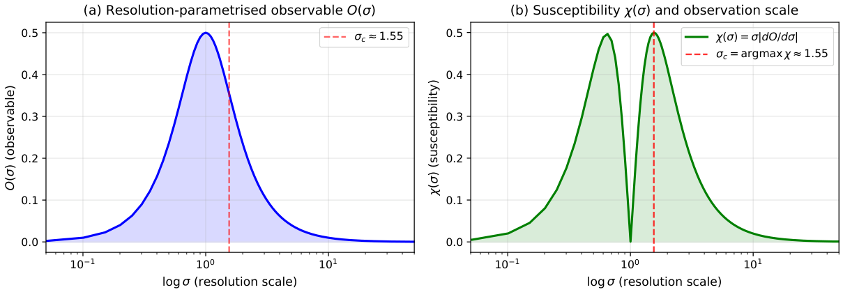
Figure 2.
Banach contraction on , with , (fixed point ). (a) Trajectory starting from . Convergence to is monotonic and geometric. (b) Distance on logarithmic scale (green) matches the predicted geometric envelope (dotted black). The vertical dashed red line marks , the characteristic geometric relaxation time of the iterate sequence. The framework’s corresponds to the first iterate (red square at ).
Figure 2.
Banach contraction on , with , (fixed point ). (a) Trajectory starting from . Convergence to is monotonic and geometric. (b) Distance on logarithmic scale (green) matches the predicted geometric envelope (dotted black). The vertical dashed red line marks , the characteristic geometric relaxation time of the iterate sequence. The framework’s corresponds to the first iterate (red square at ).
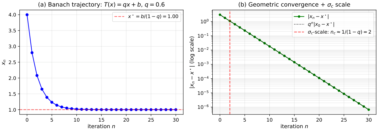
Figure 3.
Hutchinson IFS for the middle-thirds Cantor set, . (a) Iterated images for from top to bottom; convergence in Hausdorff distance to the fractal attractor is visible. (b) Box-counting function in blue (left axis) and the local box-counting exponent in green (right axis), both on log–log scales. Note that is the slope of the box-count itself and is not the susceptibility of either observable discussed in Example 5; it is plotted here as a scale-resolved estimate of dimension. is approximately constant at the Hausdorff dimension across the fractal-scaling window, which is precisely the statement that exhibits no distinguished scale there. It departs from that plateau at the small- end, where the finite-iteration approximation saturates at boxes; that departure occurs at the saturation scale , the smallest gap resolved by the iteration depth. As explained in Remark 21, is a property of the truncation and is not the observation scale; the framework’s prediction for this attractor is the upper break of (26).
Figure 3.
Hutchinson IFS for the middle-thirds Cantor set, . (a) Iterated images for from top to bottom; convergence in Hausdorff distance to the fractal attractor is visible. (b) Box-counting function in blue (left axis) and the local box-counting exponent in green (right axis), both on log–log scales. Note that is the slope of the box-count itself and is not the susceptibility of either observable discussed in Example 5; it is plotted here as a scale-resolved estimate of dimension. is approximately constant at the Hausdorff dimension across the fractal-scaling window, which is precisely the statement that exhibits no distinguished scale there. It departs from that plateau at the small- end, where the finite-iteration approximation saturates at boxes; that departure occurs at the saturation scale , the smallest gap resolved by the iteration depth. As explained in Remark 21, is a property of the truncation and is not the observation scale; the framework’s prediction for this attractor is the upper break of (26).
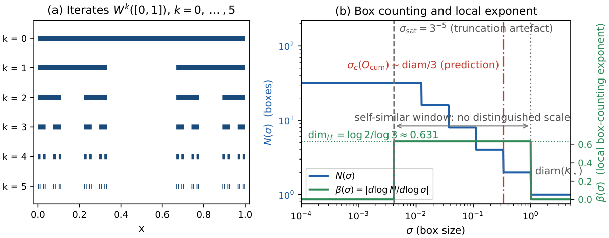
Disclaimer/Publisher’s Note: The statements, opinions and data contained in all publications are solely those of the individual author(s) and contributor(s) and not of MDPI and/or the editor(s). MDPI and/or the editor(s) disclaim responsibility for any injury to people or property resulting from any ideas, methods, instructions or products referred to in the content. |
© 2026 by the authors. Licensee MDPI, Basel, Switzerland. This article is an open access article distributed under the terms and conditions of the Creative Commons Attribution (CC BY) license (http://creativecommons.org/licenses/by/4.0/).
Copyright: This open access article is published under a Creative Commons CC BY 4.0 license, which permit the free download, distribution, and reuse, provided that the author and preprint are cited in any reuse.