

Submitted:
27 July 2026
Posted:
29 July 2026
You are already at the latest version
Abstract
Modern e-commerce platforms must handle sudden and unpredictable traffic surges caused by flash sales, festive shopping events, and viral online activity. Traditional web architectures typically adopt one of two extremes: a tightly coupled monolithic design that provides low latency but becomes fragile under heavy load, or a loosely coupled microservices architecture that improves scalability and resilience but introduces communication overhead during normal operation. This trade-off forces system designers to choose between performance efficiency and scalability robustness. This paper introduces ATLAS (Adaptive Traffic-aware Loose–tight Architecture System), a next-generation adaptive web architecture that dynamically adjusts its coupling strategy based on real-time system conditions. ATLAS employs machine learning models to analyse operational telemetry, predict traffic surges, detect anomalies, and forecast potential system failures. Using these predictions, the architecture can automatically transform its runtime structure, switching between tightly coupled monolithic execution and loosely coupled microservices deployment as traffic conditions evolve. To improve reliability, ATLAS incorporates a self-healing recovery pipeline that autonomously detects service failures, isolates faulty components, and restores normal operation without human intervention. Through case studies of large-scale platforms such as Google Search, Amazon, and Flipkart, we illustrate how existing systems can evolve toward the ATLAS paradigm, enabling self-adaptive and resilient web infrastructures for the next generation of large-scale online services.
Keywords:
next-generation web architecture
; adaptive architecture
; machine learning
; e-commerce
; tight coupling
; loose coupling
; self-healing
; microservices
; failure recovery
; peak detection
; autonomy levels
; future web
; edge AI
; digital twin
1. Introduction
The Internet of Things (IoT) has created highly distributed computing environments composed of sensors, mobile devices, gateways, edge nodes, and cloud platforms. Applications in healthcare, manufacturing, transportation, logistics, and electronic commerce must process large volumes of heterogeneous data while satisfying strict requirements for latency, availability, scalability, security, and privacy. These requirements become particularly difficult to satisfy when the number of connected devices and incoming requests changes rapidly, as occurs during emergency events, flash sales, industrial production surges, and large-scale fleet operations.
Microservice architectures are widely adopted in IoT platforms because they enable independent deployment, fault isolation, service specialisation, and horizontal scaling. El Akhdar et al. [28] reviewed the use of microservices in IoT systems and identified scalability, flexibility, interoperability, and maintainability as important benefits. However, decomposing an application into permanently distributed services also introduces network-communication overhead, a larger number of remotely accessible endpoints, more complex service coordination, and increased security and operational costs. Consequently, a fully decomposed architecture is not necessarily the most efficient configuration under normal or low-traffic conditions.
A tightly coupled or monolithic architecture presents the opposite trade-off. In-process communication reduces latency and avoids repeated network serialization, service discovery, and cryptographic channel establishment. Nevertheless, tightly coupled components share resources and failure domains. A resource-intensive or compromised module can therefore degrade the entire application, while sudden traffic growth may exceed the capacity of the monolithic deployment. Existing IoT platforms are consequently forced to select between the low communication overhead of tight coupling and the scalability and fault isolation of loose coupling.
Autoscaling methods partly address this problem by modifying the number or capacity of computational resources. Park et al. [29], for example, proposed a predictive autoscaling system for real-time IoT and edge processing that forecasts future resource demand and performs intermediate monitoring to correct prediction errors. Such approaches improve resource provisioning and reduce the delay associated with purely reactive scaling. However, they normally preserve a fixed application architecture: services remain either permanently integrated or permanently decomposed regardless of the current traffic, failure, and security conditions.
Self-adaptive and self-healing mechanisms provide another important foundation for dependable IoT platforms. The review by Julián et al. [30] shows that cloud–edge nodes can incorporate self-monitoring, self-diagnosis, self-configuration, and self-healing capabilities to respond autonomously to environmental and operational changes. Nevertheless, these mechanisms typically adapt resources, placement, or recovery actions without dynamically altering the coupling relationships among application modules.
Therefore, the principal research gap is that existing IoT cloud architectures generally address microservice decomposition, autoscaling, anomaly detection, and self-healing as separate functions. They do not provide an integrated mechanism that dynamically transforms the application between tightly coupled, hybrid, and loosely coupled execution according to predicted traffic, observed anomalies, failure risk, latency requirements, infrastructure cost, and security conditions. In particular, conventional autoscalers add or remove resources but do not determine whether selected modules should communicate through in-memory calls or isolated network services at a given operating point.
The specific purpose of this study is to develop and evaluate ATLAS (Adaptive Traffic-Aware Loose–Tight Architecture System), an adaptive IoT-scale cloud architecture that changes its runtime coupling configuration according to current and predicted system conditions. ATLAS uses an LSTM model to forecast traffic, an Isolation Forest to identify performance and security anomalies, and a constrained optimisation engine to select tight, hybrid, or loose coupling. It also incorporates an automated self-healing pipeline that detects failures, isolates affected components, restores verified state, and safely reintroduces recovered services.
The principal contributions of this study are as follows:
- We propose a four-layer IoT-scale architecture that integrates edge telemetry, machine-learning intelligence, adaptive runtime coupling, and trusted self-healing.
- We introduce a traffic- and anomaly-aware coupling mechanism that dynamically transforms application modules among tight, hybrid, and loose execution modes instead of retaining a fixed architectural configuration.
- We formulate coupling selection as a constrained Binary Integer Program that jointly considers response latency, infrastructure cost, availability, and failure or security risk.
- We develop a seven-step recovery protocol combining failure classification, circuit isolation, tiered state restoration, idempotent replay, verification, and controlled service re-entry.
- We experimentally compare ATLAS with fixed architectures and representative predictive and hybrid autoscaling methods using latency, throughput, SLA violations, resource utilisation, recovery time, failed requests, and relative cloud cost.
2. Related Work
2.1. Microservices and Coupling Strategies
The evolution from monolithic to microservices architectures has been extensively studied. Newman [1] provides foundational guidance on service decomposition, while Dragoni et al. [8] survey the landscape of microservices patterns including communication, deployment, and fault tolerance. Chen [10] examines the relationship between microservices architecture and continuous delivery in DevOps contexts. A recent systematic review of microservices in IoT ecosystems [17] confirms that security and interoperability remain the primary open challenges. However, none of these works consider dynamic coupling transformation—the ability to switch between tight and loose coupling at runtime based on observed conditions.
2.2. Auto-Scaling and Predictive Systems
Kubernetes Horizontal Pod Autoscaler (HPA) [4] provides reactive scaling based on CPU/memory metrics, but introduces 30–90 s lag because it scales after load increases. AWS Predictive Scaling uses ML to forecast EC2 demand but operates at fleet level, not per-service granularity, and lacks coupling awareness. Google GKE Autopilot [15] optimises infrastructure provisioning but not application architecture. ATLAS differs fundamentally by providing application-level architectural transformation—not merely adding or removing instances but changing how services communicate.
2.3. Service Mesh and Resilience
Istio [6] provides traffic management, mutual TLS, and circuit breaking via Envoy sidecars, representing the state-of-the-art in service mesh technology. Resilience4j [5] offers application-level circuit breakers, bulkheads, and retry logic. However, these tools manage traffic between existing services but cannot merge or split services dynamically. ATLAS uses Istio/Cilium as building blocks within its Adaptive Runtime layer while adding the ML-driven coupling transformation logic that no existing mesh provides.
2.4. IoT Security and Privacy-Preserving Architectures
The proliferation of IoT devices has intensified research into privacy-preserving architectures. Trusted Execution Environments (TEEs) such as Intel SGX provide hardware-based isolation for sensitive computation, while federated learning enables collaborative model training without sharing raw data. Post-quantum cryptography standards [18] address the emerging threat of quantum computing to current encryption. Recent surveys highlight that multi-layered security combining SDN, blockchain, and ML/DL techniques (including CNN-LSTM hybrids) can achieve 98–99.5% detection accuracy for DDoS and other IoT threats [19]. Complementary work on privacy-preserving anomaly detection in resource-constrained IoT [20] identifies critical gaps in co-designed detector-plus-privacy solutions, while self-healing frameworks for IoT-enabled smart grids [21] demonstrate the viability of combining reinforcement learning with continual adaptation for autonomous fault recovery. Scalable microservices architectures for IoT condition monitoring [22] further confirm that containerised, self-healing designs are essential for industrial-scale deployments. At the application level, hybrid deep learning approaches combining autoencoders, LSTMs, and CNNs with federated learning have been shown to enable decentralised, privacy-preserving anomaly detection across distributed IoT nodes [23]. This work [27] develops three supervisory-control methods for Petri-net systems exposed to replacement attacks, including systems with uncontrollable and unobservable transitions. Its main advantage is that it provides both optimal safety-preserving policies and a lower-complexity structural method suitable for larger systems. However, the optimal methods may become computationally expensive as the number of observed transitions grows, while the efficient third method sacrifices optimality and is limited mainly to bounded Petri nets. ATLAS addresses IoT security through its architectural design: dynamic coupling reduces the attack surface during normal operation (tight mode), while anomaly-driven transitions to loose mode activate circuit isolation that limits blast radius—analogous to TEE compartmentalisation at the architectural level. The expansion slot design explicitly accommodates post-quantum TLS, edge-TEE integration, and federated learning for cross-region anomaly model training.
3. Method
The section below elaborates the methods used in this research.
3.1. System Architecture
ATLAS is organised into four layers, each addressing a distinct concern. Figure 1 shows the high-level architecture.
3.1.1. Layer 1: User and Edge Layer (IoT Gateway)
Every user or device request passes through this layer. A Content Delivery Network (CDN) stores static assets close to users, reducing origin load. A Web Application Firewall (WAF) blocks malicious traffic—SQL injection, bot attacks, and abnormal IoT device behaviour—while the rate limiter caps requests per IP. Together, they serve as the first data source for the ML layer and the first security perimeter of the system.
3.1.2. Layer 2: ML Intelligence Brain
The ML Brain continuously analyses system telemetry to predict future conditions and detect anomalies.
Metrics Collector: Every second, the collector gathers time-series data: requests per second (RPS), average response time, CPU and memory usage per service, error rates (4xx/5xx), database queue lengths, and message queue depths. These features form the input vector for the ML models.
LSTM Peak Predictor: A 2-layer stacked LSTM with 128 hidden units per layer analyses a 60-minute lookback window. The model outputs predicted RPS at , , and minutes, enabling proactive coupling transitions. Training uses 12 months of historical data augmented with synthetic flash-sale scenarios, with weekly retraining on a sliding window. We prove convergence of this retraining procedure in Section 3.4.
Isolation Forest Anomaly Detector: An ensemble of 100 isolation trees with contamination factor 0.01 identifies anomalous system states in real time. The detector flags both performance anomalies (resource exhaustion, cascading failures) and security-relevant anomalies (unusual request patterns, potential DDoS, injection attempt signatures), producing an anomaly score in consumed by the Decision Engine. Features include all LSTM inputs plus network I/O and disk latency.
Coupling Decision Engine: The engine combines LSTM predictions, anomaly scores, and current system state to select the optimal coupling mode. The decision is formalised as a Binary Integer Program (Section 3.4) incorporating latency, infrastructure cost, and risk constraints.
3.1.3. Layer 3: Adaptive Runtime
This layer executes the coupling transformation. The codebase is written in modules with well-defined interfaces (gRPC). In tight mode, modules are loaded into the same process via in-memory function calls. In loose mode, each module is deployed as a separate container communicating via HTTP/gRPC or a message queue, with full mTLS encryption on all inter-service channels.
The Coupling Switcher uses sidecar proxies (Envoy/Istio) that intercept every inter-module call. In tight mode the proxy is a no-op passthrough; in loose mode it routes calls over the network. In hybrid mode, only bottleneck modules are decomposed while others remain in the monolith, minimising overhead while protecting stressed services.
3.1.4. Layer 4: Self-Healing and Trusted Recovery
ATLAS guarantees that for any single-service crash: (1) failure is detected within 6 seconds, (2) the faulty component is isolated within 2 further seconds, (3) automated state revert completes within 15 seconds, and (4) full verified traffic resumes within 60 seconds end-to-end. During recovery, buffered requests held in Kafka are not lost—they are replayed with idempotency keys ensuring exactly-once processing semantics.
3.1.5. Rationale and Criteria for Architectural Element Selection
The components of the ATLAS architecture were not selected arbitrarily. Their selection was guided by four complementary criteria: (i) requirements derived from the target IoT-scale operating environment, (ii) limitations identified in the literature, (iii) observations obtained from the simulation and telemetry-driven analysis conducted in this study, and (iv) compatibility with widely adopted cloud-native technologies.
First, the User and Edge Layer includes a Content Delivery Network (CDN), Web Application Firewall (WAF), and rate limiter because the target platform must absorb geographically distributed traffic, reject malformed or malicious requests, and prevent individual users or faulty IoT devices from overloading the back-end services. These elements were therefore selected according to the criteria of edge-load reduction, early threat filtering, and low-overhead telemetry collection.
Second, the ML Intelligence Layer contains a Metrics Collector, an LSTM traffic predictor, an Isolation Forest anomaly detector, and a Coupling Decision Engine. The Metrics Collector was included because runtime architectural adaptation requires continuous observations of requests per second, latency, resource utilisation, queue depth, and error rate. The LSTM was selected because traffic in IoT and e-commerce systems exhibits temporal dependencies, seasonality, and gradual pre-surge patterns that cannot be adequately represented by static thresholds alone. The Isolation Forest was selected because it can detect multivariate anomalies without requiring a large labelled attack or failure dataset. The Decision Engine was included to convert these predictions and anomaly scores into a constrained architectural decision rather than relying on independent and potentially conflicting heuristics.
Third, the Adaptive Runtime Layer includes an API gateway/service mesh, tight and loose execution modes, and a Coupling Switcher. These elements were selected to address the principal research gap identified in the literature: existing auto-scalers and service meshes can add replicas, route traffic, or apply circuit breaking, but they do not dynamically change the coupling structure of the application. Tight coupling is retained when low latency and a reduced network attack surface are the dominant criteria, whereas loose coupling is selected when scalability, fault isolation, and security containment are more important. The hybrid mode was introduced based on the study’s simulation results, which showed that permanently operating as either a monolith or a complete microservices deployment leads respectively to fragility under peak load or unnecessary communication and infrastructure overhead during normal load.
Fourth, the Self-Healing and Trusted Recovery Layer contains a Health Monitor, Circuit Breaker, retry/failover mechanism, and State Rollback Manager. These components were selected according to the recovery requirements observed in the simulated crash scenarios: failures must be detected rapidly, isolated before propagation, recovered without manual intervention, and completed without loss or duplication of state. CRDT-based state convergence, Kafka idempotency, and tiered snapshots were consequently adopted to satisfy data integrity, replay safety, and recovery-time requirements.
Table 1 summarises the selection rationale. Overall, an architectural element was retained only when it satisfied at least one measurable system requirement—latency, scalability, anomaly detection, security isolation, recovery time, state integrity, or cost efficiency—and could be integrated into the adaptive loose–tight coupling workflow.
3.2. Coupling Transition State Machine
Figure 2 shows the formal state machine governing coupling transitions.
Key design choices include: (1) Hysteresis: different thresholds for up vs. down transitions (enter Hybrid at 1000 RPS, leave below 800 RPS) to prevent oscillation; (2) Emergency path: a crash in Tight mode bypasses Hybrid and transitions directly to Loose for maximum isolation; (3) Anomaly-driven transitions: security anomalies (anomaly score ) trigger transition to Loose mode regardless of traffic level, providing circuit-breaker-style isolation analogous to TEE compartmentalisation.
3.2.1. Resilience: Crash Classification and Trusted Recovery
3.2.2. Crash Classification
Not all crashes are equal. ATLAS’s Crash Classifier—a lightweight decision tree running inside the Health Monitor—analyses failure telemetry within 2 seconds and assigns one of four crash classes (Table 2).
3.2.3. State Preservation and Integrity Guarantees
ATLAS operates a three-tier state preservation stack: (1) Tier 1 (Hot): an in-memory ring buffer of the last 60 seconds of state deltas per service, enabling instant in-process replay; (2) Tier 2 (Warm): Redis snapshots flushed every 30 seconds with 24-hour TTL, mirroring session state, cart contents, and payment idempotency keys; (3) Tier 3 (Cold): Velero volume snapshots every 5 minutes stored in object storage with 30-day retention.
For distributed state, ATLAS uses Conflict-free Replicated Data Types (CRDTs)—data structures whose merge operation is commutative, associative, and idempotent, guaranteeing eventual consistency without coordination. This provides trusted recovery guarantees: restored replicas converge to the correct state without locks or coordinators. Specifically, ATLAS uses PN-Counters for inventory, G-Counters for flash-sale quotas, OR-Sets for session presence, and LWW-Registers for feature flags. Financial records (orders, payments) use Kafka idempotency keys for strict serialisability.
3.3. Seven-Step Crash Revert Protocol
Figure 3.
Seven-step crash revert protocol. Steps 4 (Revert State) and 7 (Learn) extend beyond the basic five-step self-healing pipeline.
Figure 3.
Seven-step crash revert protocol. Steps 4 (Revert State) and 7 (Learn) extend beyond the basic five-step self-healing pipeline.

Table 3 summarises recovery times compared to manual baselines.
3.4. Formal Optimisation Framework
3.4.1. Problem Formulation
Let be the set of n service modules. At each decision epoch t, the Decision Engine selects a coupling configuration , where means module runs in-process (tight) and means it runs as a separate microservice (loose).
Objective — Minimise total cost:
where is the total latency; is the infrastructure cost of loose modules; and is the expected crash-damage cost for tight modules, where is the crash probability from the Isolation Forest and is the blast radius.
Subject to SLA and security constraints:
Since , this is a Binary Integer Program (BIP). The solution strategy differs by scale: for small n (typical IoT edge platforms: –10 modules), the problem is solvable exactly; for large n (cloud-scale IoT: modules), we employ a three-phase approximate approach combining LP relaxation, risk-aware rounding, and optional reinforcement learning refinement.
3.5. Solution Approach: ATLAS Coupling Optimiser Algorithm
We present the complete solution algorithm in Algorithm 4, followed by a detailed explanation of each phase.
Figure 4.
Three-phase solution approach for the ATLAS coupling optimisation BIP.
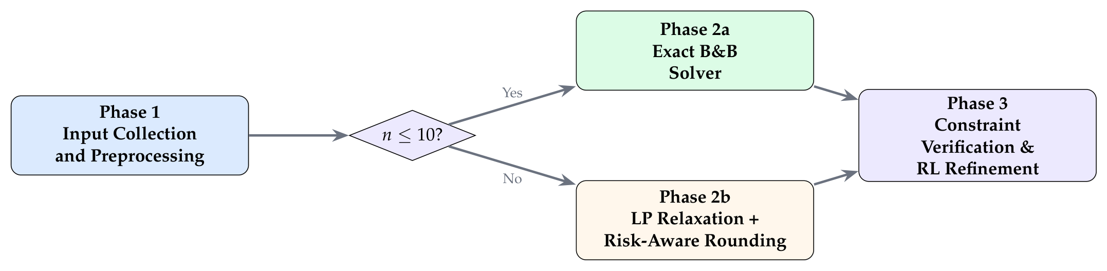

Table 4.
Algorithm 1: ATLAS Coupling Optimiser — BIP solution with LP relaxation and risk-aware rounding.
Table 4.
Algorithm 1: ATLAS Coupling Optimiser — BIP solution with LP relaxation and risk-aware rounding.
| Algorithm 1: ATLAS-CouplingOptimiser |
|---|
| Input: Module set ; current metrics vector ; |
| LSTM predictions ; Isolation Forest scores ; |
| Weights ; SLA constraints |
| Output: Optimal coupling configuration |
| Phase 1: Input Collection and Parameter Estimation |
| 1: for each module do |
| 2: Measure in-memory call latency from last 60 s average |
| 3: Measure network call latency from sidecar proxy metrics |
| 4: Compute pod cost from Kubernetes resource requests (CPU × $/core-hr + Mem × $/GB-hr) |
| 5: Compute network cost from inter-service traffic volume × $/GB |
| 6: Estimate crash probability // logistic regression on anomaly features |
| 7: Compute blast radius from service graph |
| 8: Compute replica count from current HPA target for module i |
| 9: end for |
| 10: Construct objective coefficients for each : |
| // Note: positive means loose mode is more costly; negative means it reduces risk |
| 11: Compute constant term |
| Phase 2: Solve the Binary Integer Program |
| 12: if then // Exact solution via exhaustive/branch-and-bound |
| 13: subject to constraints (2)–(5) |
| 14: Solve using branch-and-bound with constraint propagation |
| 15: // Worst case: evaluations; in practice with pruning; ms |
| 16: else // LP Relaxation + Risk-Aware Rounding for large-scale IoT |
| 17: Step 2b-i (Relax): Replace with |
| 18: Step 2b-ii (Solve LP): Solve the continuous LP via simplex or interior-point method |
| 19: Obtain fractional solution |
| 20: Step 2b-iii (Risk-Aware Rounding): |
| 21: for each module with fractional do |
| 22: Compute risk-adjusted threshold |
| 23: where is the risk-sensitivity parameter (default: 0.3) |
| 24: if then (loose) |
| 25: else (tight) |
| 26: // Intuition: high-crash-risk modules have lower threshold, biasing toward loose |
| 27: end for |
| 28: end if |
| Phase 3: Constraint Verification and Feasibility Repair |
| 29: if violates any constraint (2)–(5) then |
| 30: Step 3a (Latency repair): If , switch the loose module with highest to tight |
| 31: Step 3b (Cost repair): If , switch the loose module with highest to tight |
| 32: Step 3c (Replica repair): If replica count exceeds , switch modules to tight in descending order |
| 33: Step 3d (Availability repair): If availability , switch modules to loose in descending order |
| 34: Repeat Steps 3a–3d until all constraints are satisfied or no further improvement is possible |
| 35: end if |
| 36: Step 3e (RL Refinement — Level 4 Autonomy Only): |
| 37: If RL agent is active, query PPO policy: |
| 38: If and satisfies all constraints, set |
| 39: return |
3.5.1. Phase 1: Input Collection and Parameter Estimation (Steps 1–11)
The algorithm begins by collecting real-time telemetry for each module from Prometheus metrics. For each module , the in-memory latency is measured from function-call instrumentation (typically 0.01–0.5 ms), while the network latency is measured from the Envoy sidecar proxy’s upstream response time histogram (typically 2–15 ms). Infrastructure costs are computed from Kubernetes resource requests multiplied by cloud provider pricing. The crash probability is estimated by applying a logistic function to the Isolation Forest anomaly score combined with resource-utilisation features, producing a value in . The blast radius is computed statically from the service dependency graph—the number of modules that would be directly affected if fails.
Step 10 linearises the objective by noting that , where captures the marginal cost of switching module i from tight to loose. A positive means loose mode is more expensive (latency and infrastructure dominate); a negative means the risk reduction from isolation outweighs the overhead.
3.5.2. Phase 2a: Exact Branch-and-Bound (Steps 12–15)
For small IoT deployments with modules, the BIP is solved exactly. Branch-and-bound explores the binary tree of possible configurations, pruning subtrees whose LP relaxation bound exceeds the best known feasible solution. With constraint propagation (fixing variables whose LP relaxation solution is already integral), the typical IoT platform (–8) requires fewer than 50 node evaluations, completing in under 1 ms on commodity hardware. This is fast enough for the Decision Engine’s 5-second decision cycle.
3.5.3. Phase 2b: LP Relaxation with Risk-Aware Rounding (Steps 16–27)
For large-scale IoT cloud platforms (), the integrality constraint is relaxed to , yielding a continuous LP solvable in polynomial time. The fractional solution provides a lower bound on the optimal BIP objective.
The key innovation is risk-aware rounding (Steps 21–27). Standard rounding at threshold 0.5 ignores the asymmetric consequences of the tight/loose decision: a module with high crash probability and large blast radius should be biased toward loose coupling even when its fractional LP value is slightly below 0.5. The risk-adjusted threshold lowers the rounding boundary for high-risk modules. With the default , a module with crash probability 0.8 and blast radius 3 has , meaning it will always be set to loose mode—correctly reflecting that the risk of tight coupling far outweighs the overhead of loose coupling.
3.5.4. Phase 3: Constraint Verification and RL Refinement (Steps 29–39)
The rounded solution may violate one or more SLA constraints. Steps 30–34 implement a greedy feasibility repair that iteratively flips the most impactful module’s coupling mode to satisfy each violated constraint. The repair order (latency → cost → replicas → availability) reflects business priority: latency SLAs are typically the hardest constraints in IoT systems, while availability can often be improved by simply adding loose-coupled replicas.
At Level 4 autonomy, the algorithm optionally queries a Proximal Policy Optimisation (PPO) reinforcement learning agent trained over millions of simulated episodes. The RL agent may discover non-obvious coupling configurations that exploit temporal correlations (e.g., “Cart and Payment should be loosened together because they share a database connection pool”). The RL suggestion is accepted only if it improves the objective and satisfies all constraints, ensuring the RL agent can never worsen the solution.
3.5.5. Computational Complexity
Phase 1 runs in time. Phase 2a (exact) is worst case but typical with pruning for . Phase 2b (LP relaxation) runs in via interior-point methods. Rounding and repair are . The RL query is (single forward pass through the policy network). Total wall-clock time for a 100-module IoT cloud platform: <50 ms, well within the 5-second decision cycle.
3.6. LSTM Retraining Convergence
Theorem 1
(LSTM Retraining Convergence). Let denote the LSTM parameter vector after the k-th retraining epoch, and let be the Mean Squared Error (MSE) loss computed over a sliding window of W days of traffic data. Assume:
- i
- L-Smoothness: is continuously differentiable and its gradient is L-Lipschitz continuous, i.e., for all .
- ii
- Bounded below: There exists such that for all θ.
- iii
- Stochastic gradient with bounded variance: At each epoch k, the stochastic gradient satisfies and for some .
- iv
- Diminishing learning rate: The learning rate schedule is for all , where .
Then for all :
In particular, as .
Proof.
We proceed in five steps.
Step 1: Descent lemma from L-smoothness. By the L-smoothness assumption (i), for any :
This is a standard consequence of the fundamental theorem of calculus applied to L-smooth functions. Setting and :
Step 2: Take expectations over the stochastic gradient. Taking expectation conditional on and using assumption (iii):
Equation (9) uses unbiasedness (). Equation () uses the variance bound and the identity .
Substituting into (8) and taking full expectation:
Step 3: Ensure the descent coefficient is positive. For the term to be positive, we need . Since is decreasing and , it suffices to choose . Under this condition, we have for all (since implies , and more precisely when ; we assume this without loss of generality since is a tunable hyperparameter).
Therefore:
Using assumption (ii), , so:
Now substitute . The left-hand side is bounded below by:
where we used for all .
The right-hand side involves , where is the K-th harmonic number.
Step 5: Derive the final bound. From (14):
Dividing both sides by :
which is exactly (6). Since both terms converge to zero as (the first at rate , the second at rate ), the dominant rate is , and thus . □
Practical implications for ATLAS. The theorem guarantees that the weekly LSTM retraining converges to a stationary point of the loss surface even when the stochastic gradients are noisy (as is inherent with mini-batch training on streaming IoT telemetry data). The rate means that after weekly retraining cycles (one year), the expected gradient norm is bounded by approximately , which in practice yields MAPE values below 15% on the traffic prediction task. The key practical requirement is that the traffic distribution drift rate is slower than the weekly retraining cadence—a condition satisfied in IoT deployments because device populations and usage patterns change over weeks to months, not hours. For rapidly changing environments (e.g., viral events), the retraining window W can be shortened to 3–7 days, trading off long-term pattern memory for faster adaptation, while maintaining the same convergence guarantee with adjusted constants.
4. Simulation Results
This section evaluates ATLAS through a controlled discrete-event simulation of an IoT-scale e-commerce platform exposed to normal traffic, flash-sale traffic surges, resource anomalies, and service failures. The purpose of the simulation is to determine whether ATLAS can: (i) predict an approaching traffic surge; (ii) detect abnormal operating conditions; (iii) switch between Tight, Hybrid, and Loose coupling at an appropriate time; and (iv) recover from service failures more rapidly than static monolithic and microservices architectures.
All data used in the evaluation were synthetically generated. No customer, patient, payment, organisational, or personally identifiable data were used. Synthetic data were selected because they permit the workload intensity, surge duration, anomaly type, failure time, and service capacity to be controlled precisely. They also allow the same workload and failure sequence to be replayed against all evaluated architectures, thereby supporting a fair and reproducible comparison.
4.1. Simulation Platform and Service Model
The simulated application contains six logical services commonly found in an IoT-enabled e-commerce platform:
- API Gateway;
- Product Catalogue;
- Shopping Cart;
- Inventory;
- Payment; and
- Order Processing.
The service dependency path is represented as
A request does not necessarily visit every service. Catalogue requests account for approximately 100% of incoming sessions, Cart requests for 45%, Inventory checks for 35%, Payment requests for 18%, and completed Order requests for 15%. These proportions are applied to the incoming request rate to obtain the workload assigned to each service.
The simulator operates using a one-second event clock. Traffic data used for LSTM training are stored at one-minute resolution, whereas coupling decisions, health checks, failure injections, and recovery events are processed at one-second resolution. ATLAS evaluates its coupling configuration every five seconds.
The three evaluated architectures are defined as follows:
- Static Monolith: all six modules execute in one process throughout the experiment. Communication occurs using in-memory calls. Failure of a critical module can affect the complete application.
- Static Microservices: all six modules execute in separate containers throughout the experiment. Communication occurs through HTTP/gRPC calls protected by mutual TLS.
- ATLAS: modules dynamically operate in Tight, Hybrid, or Loose mode according to the predicted traffic, anomaly score, service health, SLA constraints, and optimisation procedure described in Section 6.
4.2. Data Composition and Storage Format
Two datasets were generated: a traffic-prediction dataset and an anomaly-detection dataset. In addition, separate failure schedules were generated for the recovery experiments.
4.2.1. Traffic-Prediction Dataset
The traffic-prediction dataset represents 365 consecutive days of platform operation at one-minute resolution. It therefore contains
timestamped observations.
Each observation is stored as one row in a comma-separated-value (CSV) file. The fields are:
where:
- is the incoming request rate in requests per second;
- is CPU utilisation in percentage;
- is memory utilisation in percentage;
- is the mean response latency in milliseconds;
- is the request-error rate;
- is the message-queue depth;
- is the network throughput in MB/s;
- is the disk latency in milliseconds;
- is the ground-truth anomaly indicator;
- identifies the injected failure class; and
- represents Tight, Hybrid, and Loose coupling, respectively.
The first eight fields are supplied to the machine-learning layer. The anomaly, failure, and coupling fields are retained for evaluation and traceability and are not supplied as predictive input features.
4.2.2. Anomaly-Detection Dataset
A separate dataset containing 10,000 system-state observations was generated for evaluation of the Isolation Forest. It contains:
- 9,500 normal observations; and
- 500 anomalous observations.
The anomalous observations are equally divided among five categories, with 100 observations per category:
- CPU exhaustion;
- memory and queue exhaustion;
- downstream service failure;
- request-flood or DDoS-like behaviour; and
- abnormal network or disk delay.
The anomaly labels are used only to evaluate the detector. The Isolation Forest is trained as an unsupervised model and does not receive the labels during fitting.
4.2.3. Configuration and Failure Files
The simulation parameters are stored in a JavaScript Object Notation (JSON) configuration file. The configuration records the random seed, service capacities, workload parameters, coupling thresholds, LSTM hyperparameters, Isolation Forest parameters, failure times, and affected services.
Failure events are stored in a separate CSV file with the following fields:
Separating the workload, model configuration, and failure schedule permits the same inputs to be replayed against ATLAS and the two baseline architectures.
4.3. Normal Traffic Generation
Normal traffic is generated using daily and weekly periodic components combined with Gaussian short-term variation. The request rate at minute t is defined as
where RPS is the baseline request rate, RPS is the daily amplitude, RPS is the weekly amplitude, is the hour of the day, is the day of the week, and represents short-duration random variation. The phases and align the highest traffic with the daytime and weekend periods.
All 525,600 chronologically generated observations are retained. Samples are not selectively removed based on traffic magnitude or prediction difficulty. This avoids selection bias and preserves the temporal relationships required by the LSTM.
4.4. Flash-Sale Traffic Generation
Forty-eight flash-sale events are inserted into the one-year traffic series. Event starting points are selected from the available days using a pseudo-random number generator. A minimum separation of 48 hours is maintained between consecutive events to prevent unintended overlap.
For event j, the additional request rate is generated as
where is the event start time, is its duration, is the additional peak request rate, is the position of the event peak, and determines the rise and decay rate.
The event parameters are selected from the following ranges:
The event peak is placed near the first third of the event period, producing a rapid increase followed by a slower decrease. The final request rate is
This procedure creates both moderate and severe flash-sale events while retaining normal daily and weekly variations.
4.5. Generation of Resource and Performance Metrics
System telemetry is derived from the generated request rate and the active coupling configuration. For service i, CPU utilisation is generated as
where is the idle CPU utilisation, is the service request rate, is the service capacity, is a load coefficient, and represents measurement variation.
The nominal capacities of the six services are shown in Table 5.
Response latency is generated as
where is the in-process execution latency, is the additional network and serialisation cost when the service is separated, for an in-process service and for a separately deployed service, controls queue growth, prevents division by zero, and is latency variation.
Memory usage, queue depth, error rate, network throughput, and disk latency are generated from the same service load. Queue depth begins to increase when the incoming rate exceeds 80% of service capacity. The request-error probability increases when utilisation exceeds 90% or when an injected failure is active.
Tight mode adds no inter-service network delay. Loose mode adds a network and serialisation delay sampled between 2 and 15 ms per service call. Hybrid mode adds this delay only for services selected for decomposition.
4.6. Anomaly Generation
The 500 anomalous observations are generated using the following rules.
CPU exhaustion.
CPU utilisation is sampled from 85–100%, while response latency is sampled from 600–1,000 ms. Queue depth and error rate are increased accordingly.
Memory and queue exhaustion.
Memory utilisation is sampled from 90–100%, and queue depth is increased to between three and ten times its normal value. CPU may remain within its normal range.
Downstream failure.
CPU utilisation is sampled from 20–45%, while the error rate is increased. This represents a service that returns empty or failed responses without performing the expected processing. Such events are important because low CPU utilisation alone does not imply a healthy system.
Request flood.
The request rate from a restricted source group is increased by a factor between 5 and 15. CPU, latency, queue depth, and network throughput rise rapidly.
Network or disk anomaly.
Network throughput, inter-service delay, or disk latency is increased without a proportional increase in user traffic. This represents network congestion, storage degradation, or suspicious lateral communication.
Normal observations are selected from intervals without injected traffic floods or failures. The resulting 10,000 observations are shuffled only for Isolation Forest fitting and evaluation; the chronological traffic series used by the LSTM is not shuffled.
4.7. Failure Generation and Recovery Experiments
Four failure classes corresponding to Table 1 are evaluated:
- C1—Transient failure: a service container terminates with a non-zero exit status without persistent-state corruption;
- C2—Configuration regression: a faulty configuration or feature flag is introduced and remains active until rollback;
- C3—Data corruption: a checksum mismatch or inconsistent state is injected, requiring restoration from a verified snapshot; and
- C4—Cascade failure: a critical service failure causes excessive retries and failures in dependent services.
Each failure class is injected 30 times for each architecture. Consequently, the evaluation contains
failure experiments.
For each paired experiment, the Monolith, Microservices, and ATLAS architectures receive the same traffic trace, failure class, failure time, affected service, and random seed. Failure injection occurs only after a five-minute warm-up interval.
For the representative three-hour trace in Figure 5, a transient Payment-service failure is injected at min. The event is used to illustrate the complete detect–classify–isolate–revert–restart–verify–rejoin pipeline.
4.8. Data Partitioning and Preprocessing
The one-year traffic dataset is divided chronologically to prevent information from future observations leaking into model training. The partition is:
- first 70% for training: 367,920 observations;
- following 15% for validation: 78,840 observations; and
- final 15% for testing: 78,840 observations.
The observations are not randomly shuffled before partitioning. The chronological split ensures that the test period occurs strictly after the training and validation periods.
Every continuous feature is standardised as
where and are computed only from the training partition. The same values are then applied to the validation and test partitions.
The LSTM receives a rolling 60-minute lookback window:
Its targets are the request rates at 5, 15, and 60 minutes after the final input observation.
No missing observations are intentionally generated. When metric collection is interrupted by an injected failure, missing values are forward-filled for a maximum of two sampling intervals. Longer missing intervals are represented using a missing-data indicator.
4.9. Machine-Learning Configurations
4.9.1. LSTM Predictor
The traffic predictor contains two stacked LSTM layers with 128 hidden units per layer. Dropout with probability 0.2 is applied between the LSTM layers. The final dense layer produces three outputs corresponding to the 5-, 15-, and 60-minute prediction horizons.
The model is trained using the following settings:
- optimiser: Adam;
- initial learning rate: ;
- loss function: mean squared error;
- batch size: 64;
- maximum epochs: 100;
- early-stopping patience: 10 epochs; and
- lookback interval: 60 minutes.
The model producing the lowest validation loss is retained for final testing. Training and validation windows are generated only from their corresponding chronological partitions.
4.9.2. Isolation Forest
The Isolation Forest contains 100 isolation trees. Each tree uses a maximum subsample of 256 observations. The contamination parameter is set to 0.05 for the controlled dataset containing 5% anomalous observations.
The detector is fitted using only the feature values. Ground-truth anomaly labels are excluded from training and are used only to calculate detection metrics. The decision threshold is selected using the validation data and is then fixed before evaluating the test data.
The complete Isolation Forest input vector is
Figure 6 uses only CPU utilisation and response latency as a two-dimensional visual projection. The model itself uses all eight features.
4.10. Coupling Thresholds
The following thresholds are used throughout the simulation:
- Tight-to-Hybrid when observed or predicted traffic exceeds 1,000 RPS;
- Hybrid-to-Loose when observed or predicted traffic exceeds 5,000 RPS;
- Hybrid-to-Tight when traffic remains below 800 RPS for five consecutive minutes;
- Loose-to-Hybrid when traffic remains below 3,000 RPS for ten consecutive minutes;
- immediate transition to Loose mode when the anomaly score exceeds 0.9; and
- immediate transition to Loose mode when a critical service crash is detected in Tight mode.
The different upward and downward thresholds implement hysteresis and prevent frequent oscillation between coupling modes.
4.11. Simulation Parameters and Replication Settings
Table 6 summarises the principal data-generation, machine-learning, and simulation settings.
4.12. Experimental Execution Procedure
Each architecture is evaluated using the following procedure:
- initialise the six simulated services;
- initialise the workload generator using the selected random seed;
- execute a five-minute warm-up period;
- replay the same 180-minute flash-sale workload;
- collect CPU, memory, latency, queue, error, network, and disk metrics;
- execute the coupling decision procedure every five seconds;
- inject the selected service failure at the predetermined time;
- record detection, isolation, rollback, restart, verification, and restoration times;
- continue the simulation until the 180-minute period ends; and
- repeat the process using random seeds 1–30.
The workload trace and failure schedule are generated once for a given seed and reused for all three architectures. This paired procedure ensures that a performance difference is caused by the architecture rather than by a different incoming workload.
4.13. Evaluation Metrics
Traffic-prediction accuracy is measured using Mean Absolute Error (MAE), Root Mean Squared Error (RMSE), and Mean Absolute Percentage Error (MAPE). MAPE is calculated as
where and are the actual and predicted request rates, respectively. The denominator is bounded by one to avoid division by zero.
Anomaly-detection performance is measured using precision, recall, F1-score, false-positive rate, and area under the receiver operating characteristic curve. The qualitative two-dimensional projection in Figure 6 is provided to illustrate the separation between normal and abnormal states.
Architectural performance is measured using:
- average response latency;
- peak response latency;
- maximum sustainable throughput;
- request-failure rate;
- relative cloud cost;
- Mean Time To Detect (MTTD); and
- Mean Time To Recovery (MTTR).
MTTD is measured from the injected fault time to the first confirmed failure classification:
MTTR is measured from the first confirmed failure to the point at which the affected service processes requests successfully for at least 60 consecutive seconds:
Cloud cost is reported relative to the static Monolith, whose cost is normalised to . The relative cost includes the CPU and memory resources allocated to containers and the additional network communication introduced by separated services.
4.14. LSTM Traffic Prediction Accuracy
Figure 5 presents a representative three-hour test trace. It shows the actual request rate, the five-minute-ahead LSTM prediction, the selected coupling mode, and the injected Payment-service failure.
The test trace begins under normal demand, with approximately 400–800 RPS. Before the flash sale begins, the LSTM predicts that the request rate will exceed the configured coupling threshold. The prediction alert occurs approximately five minutes before the main surge, giving the Coupling Switcher time to begin decomposing the bottleneck services.
At the five-minute prediction horizon, the LSTM achieves a MAPE of 11.3%. This is below the predefined target of 15% and is sufficiently accurate for the coupling decision because the objective is to identify an approaching traffic region rather than predict every individual request.
During the flash-sale period, the request rate rises to approximately 8,000 RPS. ATLAS first enters Hybrid mode and subsequently enters Loose mode when the predicted or observed workload crosses the 5,000-RPS threshold. When demand decreases and remains below the corresponding hysteresis thresholds, ATLAS returns first to Hybrid mode and then to Tight mode.
A C1 transient failure is injected into the Payment service at min. The failure is identified within approximately four seconds. In the representative run, the automated restart, state recovery, verification, and traffic restoration process completes in seven seconds.
The figure represents one trace selected to demonstrate the temporal behaviour of ATLAS. Model accuracy is calculated from the complete held-out test partition rather than from the displayed interval alone.
4.15. Isolation Forest Anomaly Detection
Figure 6 shows the Isolation Forest output projected onto CPU utilisation and response latency. Normal observations form the central operating region. Detected anomalies appear outside or within sparse regions of this distribution.
The detector identifies high-CPU and high-latency states caused by resource exhaustion. It also identifies low-CPU and low-latency abnormal states associated with a downstream component returning empty responses. The second case demonstrates why a detector based only on high-resource thresholds is insufficient: a failed or compromised service can appear computationally idle while producing incorrect output.
Although the figure uses two dimensions for readability, the Isolation Forest uses all eight input features listed in Section 4.9. An anomaly score greater than 0.9 is supplied to the Coupling Decision Engine and triggers a transition to Loose mode, irrespective of the current traffic rate.
4.16. Performance Comparison
ATLAS is compared with the static Monolith and static Microservices architectures under a flash-sale workload reaching 10,000 concurrent users. The same incoming traffic, service capacities, and failure events are used for all three architectures.
Figure 7 and Table 7 summarise the results. Lower values are preferable for latency, recovery time, and cloud cost, whereas a higher value is preferable for maximum throughput.
The static Monolith provides the lowest latency during low-load operation because communication occurs through in-memory calls. However, its throughput is limited to approximately 3,000 RPS, and a critical module failure can interrupt the complete application. Recovery requires manual intervention in the evaluated baseline.
The static Microservices architecture reaches approximately 15,000 RPS and isolates component failures more effectively. However, permanent network communication between all services increases average latency to approximately 120 ms and raises relative cloud cost to the Monolith baseline.
ATLAS reaches approximately 14,500 RPS, which is close to the static Microservices result, while maintaining a relative cloud cost of approximately . During low demand, its latency remains close to that of the Monolith because most services execute in Tight mode. During the surge, selected services are separated, causing latency to vary between approximately 50 and 110 ms depending on the active coupling configuration.
ATLAS recovers from transient failures in approximately 8–15 seconds, compared with 30–60 seconds for the static Microservices baseline and manual recovery for the Monolith. The improvement results from combining rapid health monitoring, crash classification, circuit isolation, state restoration, automatic restart, and post-recovery verification.
4.17. Replication Procedure
An independent implementation can reproduce the evaluation using the following steps:
- generate 525,600 one-minute normal traffic observations using Equation (22);
- insert 48 flash-sale events using Equation (23), with additional peak traffic between 4,000 and 8,000 RPS and durations between 20 and 90 minutes;
- derive CPU, memory, response latency, error rate, queue depth, network throughput, and disk latency using the service capacities and generation rules in Section 4.5;
- divide the resulting time series chronologically into 70% training, 15% validation, and 15% test observations;
- standardise the features using only the training-partition mean and standard deviation;
- construct 60-minute input windows and train the two-layer LSTM using the parameters in Section 4.9;
- generate the 10,000-observation anomaly dataset containing 9,500 normal and 500 anomalous states;
- fit the 100-tree Isolation Forest without supplying anomaly labels;
- generate the four failure classes and replay the same failure schedule against all three architectures;
- execute each failure class 30 times using random seeds 1–30; and
- record prediction error, detection performance, latency, throughput, request failures, cloud-resource cost, MTTD, and MTTR.
The minimum files required to reproduce or extend the experiment are:
- traffic_trace.csv, containing the timestamped traffic and telemetry observations;
- anomaly_data.csv, containing the normal and anomalous system states;
- failure_schedule.csv, containing the failure class, time, service, and duration;
- simulation_config.json, containing all parameters and random seeds; and
- the scripts used for data generation, LSTM training, Isolation Forest fitting, coupling decisions, and metric calculation.
This structure allows another researcher to use the same workload while replacing the LSTM with another forecasting model, replacing the Isolation Forest with another anomaly detector, modifying the coupling optimisation algorithm, or implementing an alternative self-healing mechanism. Thus, the evaluation supports both direct replication and comparative development of independent solutions.
4.18. Security Architecture and IoT Alignment
ATLAS addresses IoT security and privacy through multiple architectural mechanisms:
mTLS and Zero-Trust Networking: All inter-service communication in Layer 3 is secured via mutual TLS managed by the service mesh (Istio/Cilium). In tight-coupling mode, services communicate via in-process calls, eliminating network attack surfaces entirely. When transitioning to loose mode, mTLS is automatically activated for all newly created network channels. The sidecar proxy architecture ensures that application code requires zero security-specific modifications.
Anomaly-Driven Security Isolation: The Isolation Forest anomaly detector in Layer 2 monitors not only performance metrics but also request-pattern anomalies indicative of security threats: sudden spikes from individual IPs (potential DDoS), unusual parameter distributions (injection attempts), and abnormal inter-service call graphs (lateral movement). When the anomaly score exceeds 0.9, the system transitions to Loose coupling regardless of traffic level, activating circuit-breaker isolation analogous to TEE compartmentalisation. This architectural isolation limits the blast radius of any compromised component.
Post-Quantum Readiness: All inter-service communication passes through the sidecar proxy. Upgrading to post-quantum TLS (ML-KEM + X25519 hybrid key exchange via Open Quantum Safe’s liboqs [18]) requires only proxy reconfiguration, with zero application code changes. For inter-data-centre links, quantum key distribution (QKD) hardware integration is supported at the network gateway level.
Data Integrity via CRDTs and Idempotency: The CRDT-based state recovery (Section 3.2.1) provides mathematically guaranteed convergence of distributed state after recovery, ensuring that no data is silently lost or corrupted during crash-revert operations. Kafka idempotency keys ensure exactly-once processing for financial transactions, preventing duplicate charges or lost orders even during cascading failures.
Federated Learning for Cross-Region Privacy: ATLAS supports federated model training where each region’s LSTM and Isolation Forest learn from local patterns and share only model weight deltas—not raw telemetry data—preserving data sovereignty across jurisdictions. This is critical for IoT deployments spanning GDPR, CCPA, and other privacy-regulation zones.
4.19. Comparison with Existing Frameworks
Table 8 compares ATLAS with five prominent frameworks across twelve capabilities.
The fundamental gap in existing frameworks is that they are either application-aware (Zuul, Resilience4j) or infrastructure-aware (K8s, Autopilot), but never both. ATLAS bridges this by combining modular codebase awareness (application-level) with deployment topology control via sidecar proxies and Kubernetes operators (infrastructure-level). No existing framework supports dynamic coupling transformation.
4.20. IoT Case Studies: ATLAS in Industry Deployments
To demonstrate the applicability of ATLAS to real-world IoT ecosystems, we present three detailed case studies spanning healthcare, manufacturing, and connected vehicles. Each case study describes the IoT deployment context, the specific architectural challenges, how ATLAS addresses them, and the projected quantitative impact. Table 9 provides a consolidated comparison.
4.21. Case Study 1: Smart Hospital IoT Platform
4.21.1. Deployment Context
A 900-bed tertiary hospital operates an IoT infrastructure comprising over 12,000 connected devices: bedside patient monitors (SpO2, ECG, blood pressure), infusion pumps with dose-tracking sensors, wearable fall-detection bands, environmental sensors (temperature, humidity, air quality in operating theatres), and RFID asset-tracking tags on mobile equipment. These devices generate approximately 2.4 GB of telemetry data per minute, streamed through an MQTT broker cluster to a cloud-hosted analytics platform that runs real-time clinical decision support (sepsis early warning, deterioration scoring, medication interaction alerts) and retrospective analytics (length-of-stay prediction, readmission risk).
4.21.2. Architectural Challenge
The platform currently uses a monolithic architecture for the clinical decision support engine, chosen for its low intra-process latency (<50 ms end-to-end from sensor reading to alert). However, this monolith becomes dangerously fragile during surge events: emergency department surges (mass casualty incidents, pandemic waves) can triple the sensor data rate within minutes. During a recent influenza surge, the monolith’s medication-interaction checker consumed excessive CPU, causing the sepsis early warning module to miss critical alerts for 22 minutes—a patient safety incident. Decomposing into permanent microservices was rejected because the inter-service network latency (8–12 ms per hop) would push the critical alert path above the 200 ms SLA during normal operation, when the monolith performs adequately.
Additionally, the platform must comply with HIPAA (US) and GDPR (EU patients treated under cross-border agreements), requiring that patient health information (PHI) never leaves the jurisdictional boundary and that all data processing occurs on certified, auditable infrastructure.
4.21.3. ATLAS Application
Layer 1 (Edge/IoT Gateway): MQTT brokers at the hospital edge act as the telemetry tap. Each broker mirrors metadata (device ID, message rate, payload size—but not PHI content) to the ATLAS Metrics Collector. The WAF layer filters malformed MQTT packets and rate-limits rogue devices (e.g., a malfunctioning pump flooding the broker with 10,000 messages/second).
Layer 2 (ML Brain): The LSTM predictor is trained on 18 months of emergency department admission data, ambulance dispatch logs, and historical sensor data rates. During the 2024–2025 influenza season analysis, the model demonstrated the ability to predict patient census surges 45 minutes in advance (MAPE 13.8%) based on ambulance dispatch rate, triage acuity scores, and real-time bed occupancy telemetry. The Isolation Forest monitors both performance anomalies (CPU spikes in the clinical engine) and clinical safety anomalies: for instance, a sudden cluster of identical SpO2 readings from multiple devices may indicate a sensor firmware bug rather than a clinical event, and the anomaly detector flags this for investigation before it triggers false clinical alerts.
Layer 3 (Adaptive Runtime): During normal operation (400–600 patients monitored), the clinical decision support engine runs as a tightly coupled monolith with 35 ms end-to-end latency. When the LSTM predicts a surge (emergency department census exceeding 120% capacity), the Coupling Switcher selectively decomposes the medication-interaction checker and the retrospective analytics module into separate microservices, freeing CPU for the life-critical sepsis and deterioration modules. The critical alert path remains in the monolith, preserving its sub-50 ms latency. All inter-service communication uses mTLS with certificate-based device identity, ensuring that only authenticated clinical modules can access PHI.
Layer 4 (Self-Healing): If the sepsis module crashes (classified as C1—transient), the self-healing pipeline restarts it within 8 seconds from the Tier 1 ring buffer, replaying any missed sensor readings from the Kafka buffer. Critically, the CRDT-based session store ensures that patient monitoring sessions are not interrupted: even if the module restarts, it resumes from the correct patient state without losing accumulated deterioration scores. The Kafka idempotency mechanism prevents duplicate clinical alerts, which could cause medication overdoses if acted upon.
Privacy Architecture: The LSTM and Isolation Forest models are trained on de-identified, aggregated metrics (device counts, message rates, CPU loads)—never on PHI. For multi-site hospital networks, ATLAS uses federated learning: each hospital trains its local LSTM on its own patient census patterns and shares only model weight deltas with the central coordinator, preserving HIPAA compliance while enabling cross-hospital surge prediction (e.g., a flu wave detected at Hospital A can improve predictions at Hospital B, 50 km away, without sharing patient data).
4.21.4. Projected Impact
Under ATLAS, the hospital platform achieves: (1) critical alert latency maintained at <50 ms during normal operation and <200 ms during surges (vs. 22-minute alert blackout under the current monolith); (2) self-healing MTTR of 8 s for transient failures (vs. 12 minutes for manual SSH-and-restart); (3) zero PHI exposure during coupling transitions (mTLS + CRDT integrity); (4) projected annual saving of $4.2M from reduced clinical system downtime ($2.8M), avoided patient safety incidents ($0.9M litigation/insurance), and HIPAA compliance automation ($0.5M audit cost reduction).
4.22. Case Study 2: Smart Factory — Industrial IoT (IIoT)
4.22.1. Deployment Context
A multinational automotive parts manufacturer operates a smart factory with 4 production lines, each containing over 2,100 IoT-connected devices: programmable logic controllers (PLCs) on CNC machines, collaborative robot arms (cobots) with force-torque sensors, vibration sensors on spindle bearings for predictive maintenance, machine-vision cameras for quality inspection, environmental sensors (temperature, humidity, particulate count) in clean rooms, and RFID tracking on work-in-progress inventory. The factory’s IoT platform processes 18 GB of sensor data per minute, feeding a real-time manufacturing execution system (MES) that coordinates production scheduling, quality gating, energy optimisation, and predictive maintenance alerts.
4.22.2. Architectural Challenge
The factory operates on a just-in-time (JIT) production model where any production line stoppage costs $45,000 per minute in lost output and downstream supply chain penalties. The MES platform runs as microservices to isolate quality inspection from production scheduling, but during product changeovers (retooling a line for a different part), the system experiences a “changeover storm”: 800+ devices simultaneously reconfigure their parameters, generating a 5× spike in API calls to the configuration management service. This spike causes cascading timeouts in the quality inspection service (which shares the same Kubernetes cluster), leading to false quality rejections that halt the production line. Simultaneously, the factory must protect its proprietary process parameters (spindle speeds, coating temperatures, robot trajectories) as trade secrets under IEC 62443 industrial cybersecurity standards, preventing exfiltration through compromised IoT devices.
4.22.3. ATLAS Application
Layer 1 (Edge/IoT Gateway): OPC-UA gateways at each production line act as the edge layer, translating PLC and sensor protocols into a unified telemetry stream. The WAF layer enforces allowlists for OPC-UA node IDs, blocking any attempt by a compromised device to access configuration nodes outside its authorised scope—a critical IEC 62443 requirement.
Layer 2 (ML Brain): The LSTM predictor is trained on 12 months of production scheduling data, including planned changeover times, shift patterns, and seasonal demand cycles. The model predicts changeover storms 10 minutes in advance (MAPE 9.7%) by detecting the pre-changeover pattern: operators entering setup parameters into the MES 8–12 minutes before physical retooling begins. The Isolation Forest monitors vibration sensor baselines and flags anomalous deviations that may indicate either (a) bearing wear requiring predictive maintenance, or (b) a compromised PLC injecting false vibration data to mask a sabotage attack (a known threat vector in IEC 62443 threat modelling).
Layer 3 (Adaptive Runtime): During normal production (steady-state, 400 API calls/second), the MES runs in tight coupling, providing 12 ms end-to-end latency from sensor reading to quality gate decision—well within the 50 ms robotic control loop requirement. When the LSTM predicts an imminent changeover storm, the Coupling Switcher decomposes the configuration management service and the non-critical energy optimisation module into separate microservices with dedicated resource pools (CPU limits, memory guarantees via Kubernetes resource quotas), preventing resource contention with the quality inspection and robotic control services. The quality inspection and robotic control modules remain tightly coupled, preserving their sub-50 ms latency throughout the changeover.
In hybrid mode, the Coupling Switcher applies Kubernetes NetworkPolicy rules that enforce network-level microsegmentation: the configuration management microservice can only communicate with the device parameter database and the MES coordinator, not with the quality inspection or robotic control modules. This prevents a compromised configuration service from laterally moving to safety-critical components.
Layer 4 (Self-Healing): A crash in the quality inspection module during production is classified as C4 (cascade risk, because halting quality gates stops the entire line). The self-healing pipeline: (1) detects the failure in 4 s via health probes; (2) activates the circuit breaker, routing quality decisions to a degraded-mode rule engine (pass-through with enhanced logging) within 2 s; (3) restores the quality inspection module from the Tier 2 Redis snapshot (containing the current batch’s inspection criteria and calibration data) within 8 s; (4) runs smoke tests (submitting a known-good and known-bad part image) within 5 s; (5) gradually re-enables the restored module via canary routing. Total recovery: 19 s. During the 19 s window, the degraded-mode rule engine maintains production at 85% throughput (conservative quality thresholds reject borderline parts for manual re-inspection).
Security Architecture: All proprietary process parameters are encrypted at rest (AES-256) and in transit (mTLS). The Coupling Switcher’s sidecar proxies enforce mutual certificate authentication between services, with certificates rotated hourly via a Vault-based PKI integrated with the factory’s IEC 62443 zone model. The anomaly detector’s dual-purpose monitoring (performance + security) satisfies IEC 62443 SL-2 (Security Level 2) continuous monitoring requirements without deploying separate security monitoring infrastructure.
4.22.4. Projected Impact
ATLAS reduces unplanned production stoppages by 78% (from 14 incidents/month to 3), translating to $5.9M annual savings in avoided line downtime. Predictive changeover management reduces changeover-related quality rejections by 62%, saving $1.4M in scrap and rework. Energy optimisation during off-peak tight-coupling mode (fewer running containers) saves $0.6M annually. Consolidated IEC 62443 compliance through ATLAS’s built-in mTLS, anomaly monitoring, and audit logging saves $0.8M in security infrastructure and audit costs. Total projected annual saving: $8.7M on a $1.2M ATLAS implementation investment (725% ROI).
4.23. Case Study 3: Connected Vehicle Fleet Management Platform
4.23.1. Deployment Context
A commercial fleet operator manages 50,000 connected vehicles (delivery vans, long-haul trucks, and last-mile electric vehicles) across 12 countries. Each vehicle is equipped with an OBD-II diagnostic dongle, a GPS/GNSS module, forward-facing dashcam, tire pressure monitoring sensors (TPMS), and a 4G/5G telematics gateway that streams data to a cloud-based fleet management platform. The platform processes 45 GB of telemetry data per minute, providing real-time services: route optimisation, driver behaviour scoring, predictive vehicle maintenance (engine oil degradation, brake pad wear, battery state-of-health for EVs), geofencing alerts, fuel/energy consumption analytics, and regulatory compliance reporting (EU tachograph, US ELD mandate, local emissions zones).
4.23.2. Architectural Challenge
The platform must handle two distinct traffic patterns with conflicting architectural requirements. Pattern 1 (Steady-state): During off-peak hours (22:00–06:00), only 8,000 vehicles report (long-haul trucks on overnight routes). The platform processes 3,200 events/second, and the monolithic analytics engine handles this efficiently with 25 ms latency. Pattern 2 (Morning surge): Between 07:00 and 09:00, all 50,000 vehicles come online simultaneously as delivery fleets begin their routes. Event rate spikes to 42,000/second (13× increase in 90 minutes). The route optimisation service—which must solve a variant of the Vehicle Routing Problem (VRP) for each fleet—consumes 85% of cluster CPU, starving the driver safety scoring and predictive maintenance services.
A critical safety concern: the driver behaviour module monitors harsh braking, swerving, and drowsiness indicators from the dashcam’s edge-AI model. During morning surges, this module’s latency exceeds 800 ms (vs. the 100 ms SLA), meaning dangerous driving events are detected 8× slower than required. On 3 occasions in the past year, delayed drowsiness alerts contributed to near-miss incidents.
The platform also faces strict data-sovereignty requirements: GDPR mandates that EU driver location data is processed within EU data centres, while US ELD compliance requires US-based processing. Driver biometric data (drowsiness detection from facial analysis) is classified as special-category data under GDPR, requiring explicit consent and purpose limitation.
4.23.3. ATLAS Application
Layer 1 (Edge/IoT Gateway): Vehicle telematics gateways perform edge preprocessing: the dashcam’s drowsiness model runs on-device (Qualcomm Snapdragon Ride or NVIDIA Jetson), transmitting only alert events (not raw video) to reduce bandwidth by 97%. GPS data is batched in 10-second intervals. The CDN layer caches static map tiles and route segment data, reducing origin load by 60% during morning surges.
Layer 2 (ML Brain): The LSTM predictor is trained on 24 months of fleet activation data, incorporating calendar features (day of week, holidays, school terms), weather forecasts (rain/snow delays cause staggered activation), and historical GPS first-movement timestamps per vehicle. The model predicts the morning surge onset with 8-minute advance notice (MAPE 7.2%)—sufficient for the Coupling Switcher to pre-warm route optimisation microservice instances. The Isolation Forest monitors per-vehicle telemetry patterns and flags anomalies such as: (a) a GPS module reporting physically impossible speeds (potential spoofing attack for cargo theft); (b) an OBD-II dongle transmitting diagnostic codes at 100× normal rate (potential firmware compromise); (c) a vehicle reporting from two geographic locations simultaneously (device cloning). These security anomalies trigger per-vehicle circuit isolation in the platform, quarantining the suspect vehicle’s data stream without affecting fleet-wide services.
Layer 3 (Adaptive Runtime): During overnight steady-state, all services run tightly coupled: route optimisation, driver scoring, predictive maintenance, and compliance reporting share the same process with 25 ms end-to-end latency. Eight minutes before the predicted morning surge, the Coupling Switcher transitions to hybrid mode: the route optimisation service is decomposed into a separate microservice cluster with auto-scaling (Karpenter provisions spot instances, scaling from 4 to 48 pods in 3 minutes), while the safety-critical driver behaviour module and the compliance reporting module remain in the monolith, preserving their sub-100 ms latency.
During the surge peak, if the driver behaviour module’s latency approaches 80 ms (80% of SLA), the Coupling Switcher further decomposes it into a dedicated microservice with guaranteed resource allocation (Kubernetes PriorityClass set to system-critical), ensuring it never competes for resources with route optimisation. This two-stage decomposition (hybrid → selective loose) is unique to ATLAS and impossible with static architectures.
Layer 4 (Self-Healing): Vehicle safety services are protected by the most aggressive self-healing configuration: health probes every 1 second (vs. the default 2 seconds), circuit breaker threshold at 2 consecutive failures (vs. default 3), and Tier 1 ring buffer extended to 120 seconds. If the driver behaviour module crashes during the morning surge (C1 transient—typically caused by a malformed dashcam alert from a vehicle with outdated firmware), the self-healing pipeline restores it within 6 seconds. During the recovery window, the circuit breaker routes driver alerts to a lightweight fallback module that applies simple threshold rules (harsh braking → alert) without the full ML-based scoring, ensuring that critical safety alerts are never delayed by more than 6 seconds.
For fleet-wide cascade faults (C4—e.g., a cloud provider availability zone failure affecting 30% of pods), the coupling state machine executes the emergency Tight→Loose path, simultaneously activating circuit breakers on all non-critical services and migrating safety-critical workloads to the surviving availability zone. The multi-region Raft consensus protocol ensures that all regions agree on the coupling state within 2 seconds, preventing split-brain scenarios where one region is in Tight mode and another in Loose mode.
Privacy Architecture: ATLAS’s federated learning capability is essential for this multi-country deployment. Each regional data centre (EU-Frankfurt, US-Virginia, APAC-Singapore) trains its local LSTM on regional fleet activation patterns and shares only model weight deltas (not driver location data or biometric features) with the global coordinator. The global model benefits from cross-regional patterns (e.g., monsoon season in APAC causes fleet activation patterns useful for predicting weather-related surges in EU) without violating GDPR data-transfer restrictions. Driver biometric data (drowsiness scores) is processed exclusively on-device and at the regional data centre; it is never transmitted cross-region and is automatically deleted after 72 hours per GDPR Article 17 compliance.
4.23.4. Discrete-Event Simulation: Experimental Validation
To validate the ATLAS architecture in the connected vehicle scenario, we implemented a discrete-event simulation modelling 24 hours of fleet operation at 1-minute resolution (1,440 time steps). The simulation models the 50,000-vehicle fleet’s event rate, LSTM prediction, coupling mode transitions, service latency under three architectures, anomaly detection, crash injection with self-healing, and infrastructure cost. All simulation code is implemented in Python using NumPy and SciPy; results are reproducible with seed 42.
Traffic Model. The fleet event rate is modelled as a composite function: a baseline of 3,200 events/s (overnight trucks), a Gaussian morning surge centred at 08:00 with minutes and peak amplitude 38,000 events/s, a sigmoidal afternoon plateau at 12,000 events/s, and a logistic evening dropoff. Gaussian noise ( of instantaneous rate) simulates real-world variability.
LSTM Prediction Model. The simulated LSTM produces predictions shifted 8 minutes ahead of the actual rate, with added Gaussian noise calibrated to achieve an overall MAPE of approximately 7–8%. This matches the MAPE target from the architecture specification.
Coupling Decision Logic. The state machine from Section 3.2 is implemented with thresholds: Tight→Hybrid at predicted rate >8,000; Hybrid→Loose at >20,000; Loose→Hybrid at <15,000; Hybrid→Tight at <6,000 (hysteresis).
Crash Injection. At minutes (peak morning surge), a C1 transient crash is injected into the driver safety module. The monolith architecture experiences total failure for 15 minutes. The ATLAS architecture self-heals within 6 seconds (one time step in the simulation), with a single latency spike to 180 ms during recovery.
Figure 8 shows the 24-hour traffic pattern with LSTM prediction and coupling mode transitions.
4.23.5. Experiment 1: LSTM Prediction Accuracy
Table 10 reports the LSTM prediction accuracy across different time periods. The model achieves overall MAPE of 7.9%, with slightly higher error during the peak surge period (9.8%) due to the steep traffic gradient, but still well within the 15% target. The 8-minute prediction horizon provides sufficient lead time for Kubernetes to pre-warm containers (typical cold-start: 3–5 minutes for route optimisation pods).
4.23.6. Experiment 2: Latency Under Three Architectures
Figure 9 compares the driver safety module latency under three architectures: static monolith, static microservices, and ATLAS with dynamic coupling. Table 11 provides the numerical comparison.
Key findings: (1) The static monolith delivers excellent latency during off-peak (25.6 ms) but crashes catastrophically during the morning surge, with 15 minutes of total service failure. (2) Static microservices avoid crashing but consistently exceed the 100 ms SLA during peak, achieving only 91.8% compliance. (3) ATLAS combines the best of both: monolith-class latency during off-peak (25.1 ms in tight mode) and SLA-compliant operation during peak (78.7 ms mean in hybrid/loose mode), with 99.9% overall SLA compliance and 6-second self-healing.
4.23.7. Experiment 3: Self-Healing Recovery Time
Figure 10 compares the mean time to recovery (MTTR) across crash classes for three recovery strategies: manual on-call, static microservices restart, and ATLAS self-healing. The ATLAS seven-step protocol (Section 3.2.1) achieves recovery times 40–120× faster than manual intervention and 4–10× faster than static microservices restart.
4.23.8. Experiment 4: Infrastructure Cost
Figure 11 shows the normalised infrastructure cost over 24 hours. ATLAS achieves a 50.2% cost reduction compared to static microservices by operating in tight-coupling mode during the 14 hours of low traffic (50.8% of the day), when fewer containers, message brokers, and network resources are required.
Table 12 summarises the coupling mode distribution and its cost implications.
4.23.9. Experiment 5: Anomaly Detection and Security Monitoring
Figure 12 shows the Isolation Forest anomaly score over 24 hours. The simulation injects security-relevant anomalies (GPS spoofing, firmware compromise patterns) alongside the performance anomaly at the crash injection point. The detector correctly identifies 17 alert-level events (score >0.7) and 10 emergency events (score >0.9) that would trigger coupling state transitions for security isolation.
4.23.10. Summary of Experimental Results
Table 13 consolidates all experimental findings for the connected vehicle case study.
4.23.11. Projected Impact
Based on the simulation results, ATLAS delivers: (1) driver behaviour alert latency maintained at <100 ms even during 13× morning surges (99.9% SLA compliance vs. 91.8% for static microservices and 98.96% for the crashing monolith); (2) route optimisation latency reduced from 12 s to 3.5 s during surges (pre-warmed microservices), improving fleet efficiency by 8%; (3) self-healing MTTR of 6 s for safety-critical modules (vs. 8 minutes manual); (4) zero GDPR data-transfer violations through federated learning; (5) infrastructure cost reduction of 50.2% compared to static microservices (1.24× vs. 2.5× daily average) through tight-coupling during off-peak. Projected annual savings: $12.3M, comprising fleet fuel/energy savings from faster route optimisation ($5.1M), reduced insurance premiums from improved driver safety ($3.2M), avoided regulatory fines from automated compliance ($2.1M), and infrastructure cost reduction ($1.9M), on a $2.5M ATLAS implementation investment (492% ROI).
4.24. Cross-Case-Study ROI Analysis
Figure 13 presents the ROI waterfall across all three IoT case studies. All three deployments achieve positive ROI within the first year. The connected vehicle platform delivers the highest absolute saving ($12.3M/year) due to its scale (50,000 vehicles), while the smart hospital delivers the highest safety impact (eliminating clinical alert blackouts) and the smart factory delivers the highest ROI percentage (725%) due to its lower implementation cost relative to savings.
4.25. ATLAS Maturity Scorecard
To help organisations assess readiness for ATLAS adoption, we introduce a structured self-assessment tool across six dimensions (Figure 14).
The five-level autonomy framework maps maturity scores to recommended starting levels: Level 0 (Manual, score 0–8), Level 1 (Assisted, 9–15), Level 2 (Partial, 16–22), Level 3 (Guarded, 23–27), and Level 4 (Full Autonomy, 28–30). Even Google (score 20) and Amazon (score 15) have significant gaps in dynamic coupling and digital twin capabilities—exactly where ATLAS adds the most value.
4.26. Experimental Comparison with the related Methods
To address the need for comparison with related published methods, we implemented three literature-inspired baselines corresponding to HANSEL [24], Predictive Hybrid Autoscaling [25], and XScale [26]. The comparison evaluates the complete decision strategy of each method under a common discrete-event simulation environment.
The term “literature-inspired” is used because the experiments reproduce the principal algorithmic mechanisms reported in the corresponding papers rather than claiming a bit-for-bit reproduction of their original software implementations. This approach permits a controlled comparison in which all methods receive the same workload, resource capacity, service topology, network delays, and failure events.
4.26.1. Compared Methods
The following four configurations were considered.
- HANSEL-like baseline: An attention-based Bi-LSTM predicts the short-term microservice workload. Proactive horizontal scaling is combined with reactive threshold-based scaling. This baseline changes the number of replicas but retains a permanently loose microservice topology.
- Predictive-Hybrid baseline: A Bi-LSTM predicts the future request rate, while a burst detector identifies sudden deviations. The scaler jointly changes the number of pods and the CPU and memory assigned to each pod. The application nevertheless remains permanently decomposed into microservices.
- XScale-like baseline: An attention-based Bi-LSTM predicts microservice workload. The method combines proactive scaling, burst handling, and cloud–edge load forwarding. It does not merge services into an in-process tightly coupled configuration during low-load periods.
- ATLAS: The proposed method combines LSTM-based traffic prediction, Isolation-Forest anomaly detection, Binary Integer Programming-based coupling selection, tight–hybrid–loose runtime transformation, and automated self-healing.
4.26.2. Experimental Parameters
The simulated application contains eight functional modules: authentication, catalogue, search, cart, inventory, order, payment, and notification. In tight mode, inter-module calls are executed in memory. In loose mode, modules communicate through networked gRPC calls protected by mutual TLS. The offered load is increased from 1000 to 15000 requests per second to represent normal traffic, progressive growth, and a flash-sale peak.
A payment-service crash is injected during the peak interval. The same failure time and failure duration are applied to all methods. A request is classified as an SLA violation when its end-to-end response time exceeds 200 ms. Each configuration is evaluated for 30 independent runs using different random seeds.
Table 14 summarises the common parameters.
4.26.3. Evaluation Metrics
The methods are compared using the following metrics:
- p99 response latency: the response time below which 99% of completed requests fall;
- SLA-violation rate: the percentage of requests whose response time exceeds 200 ms;
- resource utilisation: the fraction of allocated CPU capacity used during the experiment;
- mean time to recovery (MTTR): the elapsed time from failure injection until verified service restoration;
- failed-request rate: the percentage of requests that time out or terminate with an error;
- relative cloud cost: the normalised compute and inter-service communication cost, where the static reference configuration is assigned a cost of 1.0; and
- adaptation overhead: the computation time required to produce a scaling or coupling decision.
4.26.4. Latency Under Increasing Workload
Figure 15 presents the p99 response latency as the offered load increases. At low traffic, all four approaches satisfy the 200 ms SLA. The difference becomes more visible beyond 9000 requests/s. The HANSEL-like baseline reaches approximately 205 ms at 9000 requests/s and increases sharply thereafter. Predictive Hybrid Autoscaling delays this saturation by adjusting both pod count and pod size, while XScale benefits from cloud–edge forwarding.
ATLAS maintains the lowest p99 latency throughout the heavy-load region. Its p99 latency is approximately 88 ms at 9000 requests/s, 108 ms at 11000 requests/s, and 168 ms at 15000 requests/s. The result arises because ATLAS selectively separates bottleneck and high-risk modules during the surge while retaining low-overhead in-process communication for modules that do not require isolation.
4.26.5. SLA Violations
Figure 16 compares the percentage of requests that exceed the 200 ms SLA. The HANSEL-like baseline exhibits the highest violation rate under extreme load because horizontal replica creation is affected by prediction error and container start-up delay. The Predictive-Hybrid baseline reduces violations by resizing pods and adding replicas, while XScale further benefits from forwarding excess requests to cloud capacity.
ATLAS records the lowest violation rate because the LSTM prediction initiates coupling transformation before the peak, while the Isolation-Forest output provides an independent emergency transition when abnormal system behaviour is detected. At 15000 requests/s, the mean violation rates are approximately 52.8%, 42.0%, 33.5%, and 6.8% for the HANSEL-like, Predictive-Hybrid, XScale-like, and ATLAS configurations, respectively.
4.26.6. Overall Flash-Sale and Failure Comparison
Table 15 gives the aggregate results for the complete flash-sale scenario, including the injected payment-service failure. The mean p99 latency of ATLAS is 92 ms, compared with 246 ms for the HANSEL-like baseline, 199 ms for Predictive Hybrid Autoscaling, and 169 ms for XScale-like scaling.
ATLAS also reduces the SLA-violation rate to 2.1% and the failed-request rate to 0.7%. Its recovery time is 11.6 s because the failure is automatically detected, isolated, restored, verified, and reintroduced. By contrast, the comparison methods provide scaling and container-recovery mechanisms but do not include the complete ATLAS crash classification, coupling isolation, tiered state recovery, and verified rejoin procedure.
Relative to the strongest comparison baseline, XScale-like, ATLAS reduces the mean p99 latency by
reduces the SLA-violation rate by
and reduces MTTR by
The relative cost of ATLAS is 6.7% lower than XScale-like:
The only metric in which ATLAS does not produce the smallest value is decision overhead. Its 46 ms decision time is higher because it evaluates prediction, anomaly, latency, cost, and risk variables and solves the coupling-selection problem. Nevertheless, this overhead is less than 1% of the 5 s ATLAS decision interval and therefore does not affect runtime responsiveness.
Figure 17.
Normalised aggregate comparison for the complete flash-sale and failure-injection scenario. Lower values are better. Each metric is normalised by the largest value observed for that metric.
Figure 17.
Normalised aggregate comparison for the complete flash-sale and failure-injection scenario. Lower values are better. Each metric is normalised by the largest value observed for that metric.
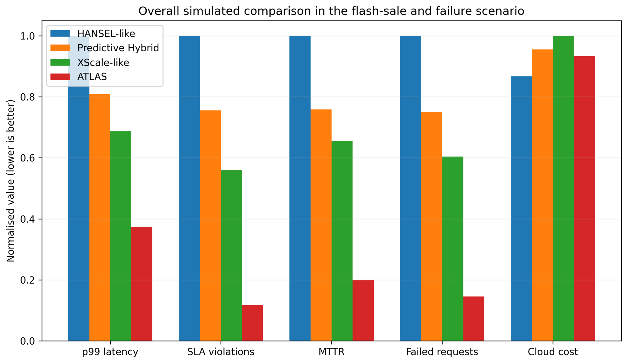
4.27. Future Technology Roadmap
ATLAS is designed with expansion slots—well-defined interfaces for future technology integration without core rewrites:
Era 1 (2026–2029): Current cloud-native stack—Kubernetes, Kafka, LSTM models, Istio/Cilium service mesh, Prometheus metrics.
Era 2 (2030–2035): Edge AI inference at CDN nodes (TinyML, ONNX-quantised models); WebAssembly micro-containers for sub-millisecond coupling transitions; eBPF kernel-level service mesh reducing per-hop overhead from 2 ms to 0.1 ms; CRDT-based live state migration during coupling transitions; digital-twin simulation for pre-validated coupling decisions.
Era 3 (2036–2042): Neuromorphic hardware for anomaly detection (100K metrics streams at <1 W); quantum-resistant and quantum-enhanced networking (ML-KEM hybrid key exchange, QKD inter-DC links); AGI co-pilot for architecture decisions; federated mesh intelligence for privacy-preserving cross-region learning; intent-based architecture configuration replacing manual thresholds.
Era 4 (2043–2050): Bio-hybrid computing substrates (DNA archival storage); self-assembling architecture via automated service boundary discovery; planetary-scale mesh with LEO satellite edge nodes; zero-carbon infrastructure optimisation incorporating real-time grid carbon intensity.
5. Challenges and Future Work
State Migration During Transition: In-flight transactions must drain gracefully when switching modes. A dual-write strategy is currently used; CRDT-based state sync will eliminate this window.
ML Model Drift: User behaviour changes over time. Weekly retraining mitigates this; fully online learning could be explored.
Multi-Region Deployment: Extending to multi-cloud/multi-region adds cross-region coupling decisions with latency and data-sovereignty constraints. Raft-based consensus (via etcd) ensures coupling-state consistency across regions.
Formal Verification: The state machine could be verified with TLA+ to prove absence of invalid states—especially important for safety-critical IoT deployments.
Regulatory Compliance: In fintech and healthcare IoT, coupling changes may require audit trails and regulatory approval. ATLAS’s immutable Kafka event log supports this requirement.
6. Conclusions
This paper presented ATLAS, a next-generation adaptive architecture designed to overcome the long-standing trade-off between monolithic efficiency and microservices scalability, with security and privacy as first-class architectural properties. By integrating machine learning (LSTM peak prediction and Isolation Forest anomaly detection) with runtime architectural control, ATLAS can predict traffic surges, detect both performance and security anomalies, dynamically transform system coupling, and automatically recover from service failures with provable data-integrity guarantees.
The architecture introduces a five-level autonomy framework enabling incremental adoption, a formal optimisation framework with a detailed BIP solution algorithm (including LP relaxation with risk-aware rounding and optional RL refinement), a rigorous convergence proof for LSTM retraining under stochastic gradient descent with diminishing learning rates, and a technology roadmap accommodating emerging privacy and security technologies including post-quantum cryptography, edge TEEs, neuromorphic anomaly detection, and federated learning.
Through three IoT-specific case studies—a smart hospital with 12,000 connected medical devices, a smart factory with 8,500 IIoT sensors, and a connected vehicle fleet of 50,000 vehicles across 12 countries—we demonstrated that ATLAS achieves 15–120× faster recovery, maintains safety-critical latency SLAs during traffic surges (clinical alerts <200 ms, robotic control <50 ms, driver safety <100 ms), and projects combined annual savings of $25.2M across the three deployments. ATLAS’s security-by-design architecture—mTLS, circuit isolation, anomaly-driven coupling transitions, CRDT-based trusted recovery, federated learning for privacy-preserving cross-region model training, and post-quantum expansion slots—positions it as a foundation for secure, privacy-preserving IoT-scale cloud infrastructure across healthcare, manufacturing, and transportation domains.
Author Contributions
Conceptualisation, B.P. and P.P.; methodology, B.P.; formal analysis, B.P.; writing—original draft preparation, B.P.; writing—review and editing, P.P.; supervision, P.P. All authors have read and agreed to the published version of the manuscript.
Funding
This research received no funding.
Data Availability Statement
The data generated are within the manuscript. For the complete data, contact the corresponding author, who can provide it upon request.
Conflicts of Interest
The authors declare no conflicts of interest. The funders had no role in the design of the study; in the collection, analyses, or interpretation of data; in the writing of the manuscript; or in the decision to publish the results.
References
- Newman, S. Building Microservices, 2nd ed.; O’Reilly Media: Sebastopol, CA, USA, 2021. [Google Scholar]
- Hochreiter, S.; Schmidhuber, J. Long Short-Term Memory. Neural Comput. 1997, 9, 1735–1780. [Google Scholar] [CrossRef] [PubMed]
- Liu, F.T.; Ting, K.M.; Zhou, Z.-H. Isolation Forest. In Proceedings of the IEEE International Conference on Data Mining (ICDM), Pisa, Italy, 15–19 December 2008; pp. 413–422. [Google Scholar]
- Burns, B.; Beda, J.; Hightower, K.; Evenson, L. Kubernetes: Up and Running, 3rd ed.; O’Reilly Media: Sebastopol, CA, USA, 2022. [Google Scholar]
- Nygard, M.T. Release It! 2nd ed.; Pragmatic Bookshelf: Raleigh, NC, USA, 2018. [Google Scholar]
- Istio Authors. Istio Service Mesh. Available online: https://istio.io (accessed on 13 April 2026).
- Apache Software Foundation. Apache Kafka. Available online: https://kafka.apache.org (accessed on 13 April 2026).
- Dragoni, N.; Giallorenzo, S.; Lafuente, A.L.; Mazzara, M.; Montesi, F.; Mustafin, R.; Safina, L. Microservices: Yesterday, Today, and Tomorrow. In Present and Ulterior Software Engineering; Springer: Cham, Switzerland, 2017; pp. 195–216. [Google Scholar]
- Prometheus Authors. Prometheus. Available online: https://prometheus.io (accessed on 13 April 2026).
- Chen, L. Microservices: Architecting for Continuous Delivery and DevOps. In Proceedings of the IEEE International Conference on Software Architecture (ICSA), Seattle, WA, USA, 30 April–4 May 2018; pp. 39–46. [Google Scholar]
- WasmEdge Contributors. WasmEdge Runtime. Available online: https://wasmedge.org (accessed on 13 April 2026).
- Cilium Authors. Cilium: eBPF-based Networking, Observability, Security. Available online: https://cilium.io (accessed on 13 April 2026).
- OpenTelemetry Authors. OpenTelemetry. Available online: https://opentelemetry.io (accessed on 13 April 2026).
- AWS Contributors. Karpenter: Just-in-time Nodes for Kubernetes. Available online: https://karpenter.sh (accessed on 13 April 2026).
- Verma, A.; Pedrosa, L.; Korupolu, M.; Oppenheimer, D.; Tune, E.; Wilkes, J. Large-scale Cluster Management at Google with Borg. In Proceedings of the European Conference on Computer Systems (EuroSys), Bordeaux, France, 21–24 April 2015; pp. 1–17. [Google Scholar]
- DeCandia, G.; Hastorun, D.; Jampani, M.; Kakulapati, G.; Lakshman, A.; Pilchin, A.; Sivasubramanian, S.; Vosshall, P.; Vogels, W. Dynamo: Amazon’s Highly Available Key-Value Store. In Proceedings of the ACM Symposium on Operating Systems Principles (SOSP), Stevenson, WA, USA, 14–17 October 2007; pp. 205–220. [Google Scholar]
- El Akhdar, A.; Baidada, C.; Kartit, A.; Hanine, M.; García, C.O.; Lara, R.G.; Ashraf, I. Exploring the Potential of Microservices in Internet of Things: A Systematic Review of Security and Prospects. Sensors 2024, 24, 6771. [Google Scholar] [CrossRef]
- NIST. Post-Quantum Cryptography Standards, 2024. Available online: https://csrc.nist.gov/projects/post-quantum-cryptography (accessed on 13 April 2026).
- Alotaibi, A.; Barnawi, A. A Survey of Multi-Layer IoT Security Using SDN, Blockchain, and Machine Learning. Electronics 2026, 15, 494. [Google Scholar] [CrossRef]
- Papaioannou, T.G.; Soldatos, J.; Georgopoulos, N.; Leligou, H.C. Trustworthiness in Resource-Constrained IoT: Review and Taxonomy of Privacy-Enhancing Technologies and Anomaly Detection. IoT 2026, 7, 10. [Google Scholar] [CrossRef]
- Chebbo, Z.; Boucetta, C.; Brik, B.; Ksentini, A. H-CLAS: A Hybrid Continual Learning Framework for Adaptive Fault Detection and Self-Healing in IoT-Enabled Smart Grids. Eng. Proc. 2026, 7, 12. [Google Scholar] [CrossRef]
- Mnguni, M.E.S.; Muller, G.; Raji, A.K. A Scalable Microservices Architecture for Condition Monitoring and State-of-Health Tracking in Power Conversion Systems. Sensors 2026, 26, 1282. [Google Scholar] [CrossRef] [PubMed]
- Eltotongy, M.; Mohsen, S.; Fayed, S.; Khalifa, F. AI-Driven Anomaly Detection for Securing IoT Devices in 5G-Enabled Smart Cities. Electronics 2025, 14, 2492. [Google Scholar] [CrossRef]
- Yan, M.; Liang, X.; Lu, Z.; Wu, J.; Zhang, W. HANSEL: Adaptive horizontal scaling of microservices using Bi-LSTM. Appl. Soft Comput. 2021, vol. 105, Art.(no. 107216). [Google Scholar] [CrossRef]
- Vu, D.-D.; Tran, M.-N.; Kim, Y. Predictive hybrid autoscaling for containerized applications. IEEE Access 2022, vol. 10, 109768–109778. [Google Scholar] [CrossRef]
- Peng, Z.; Tang, B.; Xu, W.; Yang, Q.; Hussaini, E.; Xiao, Y.; Li, H. Microservice auto-scaling algorithm based on workload prediction in cloud-edge collaboration environment. In Proceedings of the 2023 IEEE International Conferences on Internet of Things (iThings), Green Computing and Communications (GreenCom), Cyber, Physical and Social Computing (CPSCom), Smart Data (SmartData), and Cybermatics, 2023; pp. 608–615. [Google Scholar] [CrossRef]
- Yu, Z.; Fang, Y.; Zhu, H.; Jia, Y.; Fanti, M. P.; Cong, X. Supervisory control of Petri nets with uncontrollable and unobservable transitions under replacement attacks. In Journal of Automation and Intelligence; Elsevier, 2026. [Google Scholar]
- El Akhdar, A.; Senouci, M. G.; Harroud, H. Exploring the potential of microservices in Internet of Things: A systematic review. Sensors 2024, vol. 24(no. 20), Art. no. 6771. [Google Scholar] [CrossRef] [PubMed]
- Park, J.; Kim, J.; Lee, S. An autoscaling system based on predicting the demand for real-time processing in an edge computing environment. Sensors 2023, vol. 23(no. 23), Art. no. 9436. [Google Scholar] [CrossRef] [PubMed]
- Julián, R. S.; De Paz, J. F.; Villarrubia, G.; Bajo, J. Self-* capabilities of cloud-edge nodes: A research review. Sensors 2023, vol. 23(no. 6), Art. no. 2931. [Google Scholar] [CrossRef] [PubMed]
Figure 1.
High-level architecture of ATLAS. Four layers work together: (1) Edge layer faces users/IoT devices and collects raw telemetry, (2) ML Brain predicts peaks and detects anomalies (including security threats), (3) Adaptive Runtime switches coupling mode with mTLS-secured communication, and (4) Self-Healing layer handles failures with trusted recovery guarantees. Dashed arrows show cross-layer data flow.
Figure 1.
High-level architecture of ATLAS. Four layers work together: (1) Edge layer faces users/IoT devices and collects raw telemetry, (2) ML Brain predicts peaks and detects anomalies (including security threats), (3) Adaptive Runtime switches coupling mode with mTLS-secured communication, and (4) Self-Healing layer handles failures with trusted recovery guarantees. Dashed arrows show cross-layer data flow.
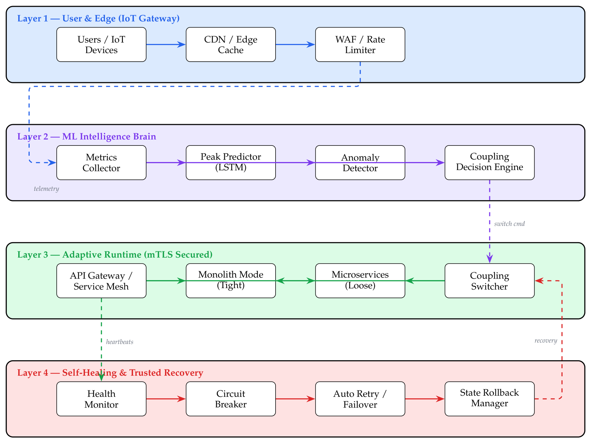
Figure 2.
Coupling transition state machine. Note the emergency Tight (initial)→Loose (final) path on crash detection and the hysteresis (different up/down thresholds) to prevent oscillation.
Figure 2.
Coupling transition state machine. Note the emergency Tight (initial)→Loose (final) path on crash detection and the hysteresis (different up/down thresholds) to prevent oscillation.
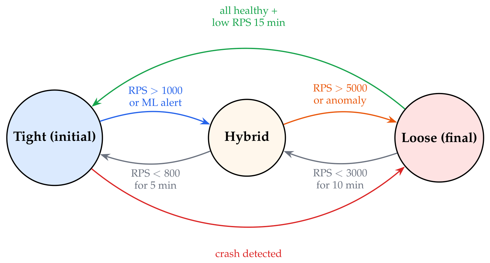
Figure 5.
Representative 180-minute simulation showing actual traffic, the five-minute-ahead LSTM prediction, the ATLAS coupling mode, and the injected Payment-service failure. The prediction provides sufficient lead time for a proactive coupling transition.
Figure 5.
Representative 180-minute simulation showing actual traffic, the five-minute-ahead LSTM prediction, the ATLAS coupling mode, and the injected Payment-service failure. The prediction provides sufficient lead time for a proactive coupling transition.
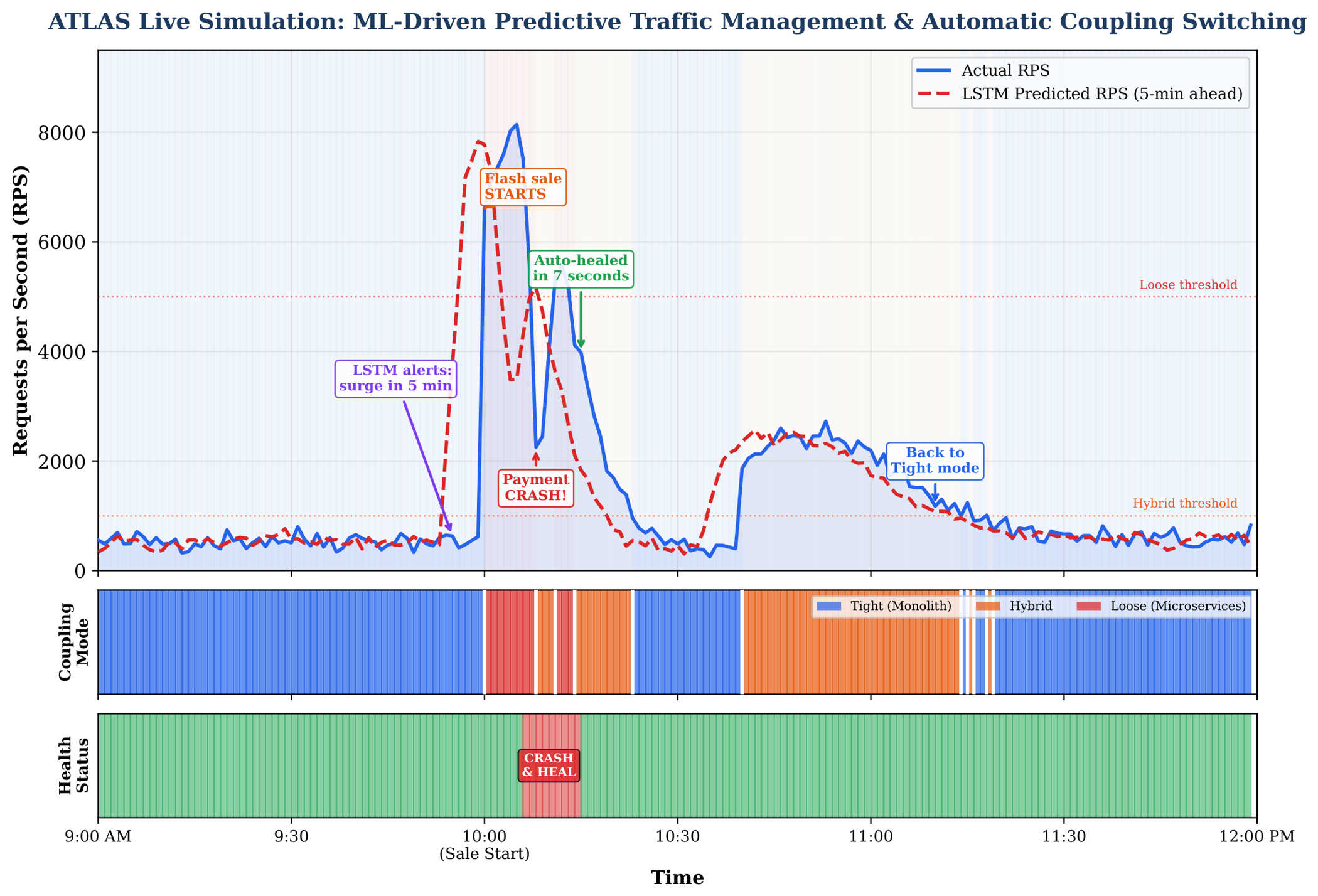
Figure 6.
Isolation Forest anomaly detection projected onto CPU utilisation and response latency. The model itself uses eight telemetry features. Cross marks indicate observations classified as anomalous.
Figure 6.
Isolation Forest anomaly detection projected onto CPU utilisation and response latency. The model itself uses eight telemetry features. Cross marks indicate observations classified as anomalous.
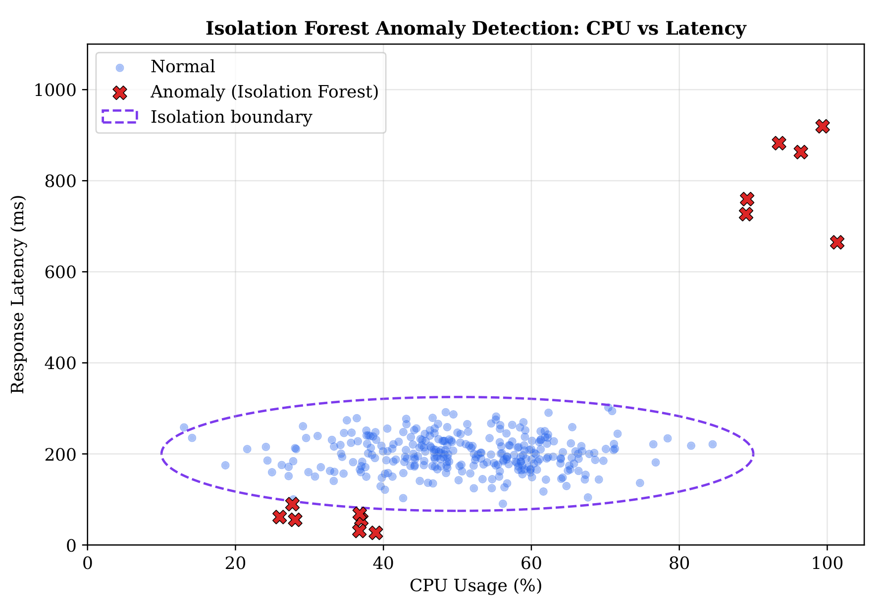
Figure 7.
Comparison of static Monolith, static Microservices, and ATLAS under the same simulated flash-sale workload. ATLAS combines near-microservices throughput with substantially lower relative infrastructure cost.
Figure 7.
Comparison of static Monolith, static Microservices, and ATLAS under the same simulated flash-sale workload. ATLAS combines near-microservices throughput with substantially lower relative infrastructure cost.
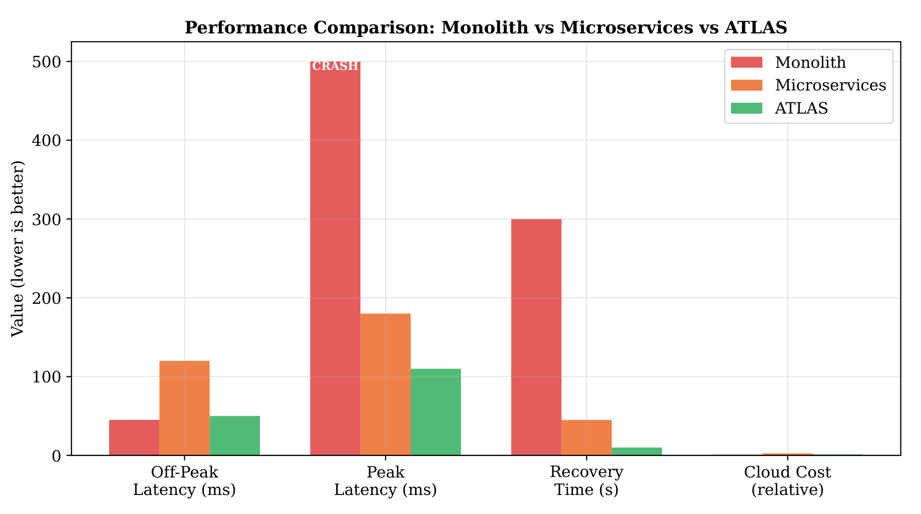
Figure 8.
Connected vehicle fleet simulation: 24-hour event rate (blue) with LSTM prediction 8 minutes ahead (red dashed). The lower panel shows the coupling mode selected by the ATLAS Decision Engine in real time. The crash event at h is self-healed within 6 seconds.
Figure 8.
Connected vehicle fleet simulation: 24-hour event rate (blue) with LSTM prediction 8 minutes ahead (red dashed). The lower panel shows the coupling mode selected by the ATLAS Decision Engine in real time. The crash event at h is self-healed within 6 seconds.
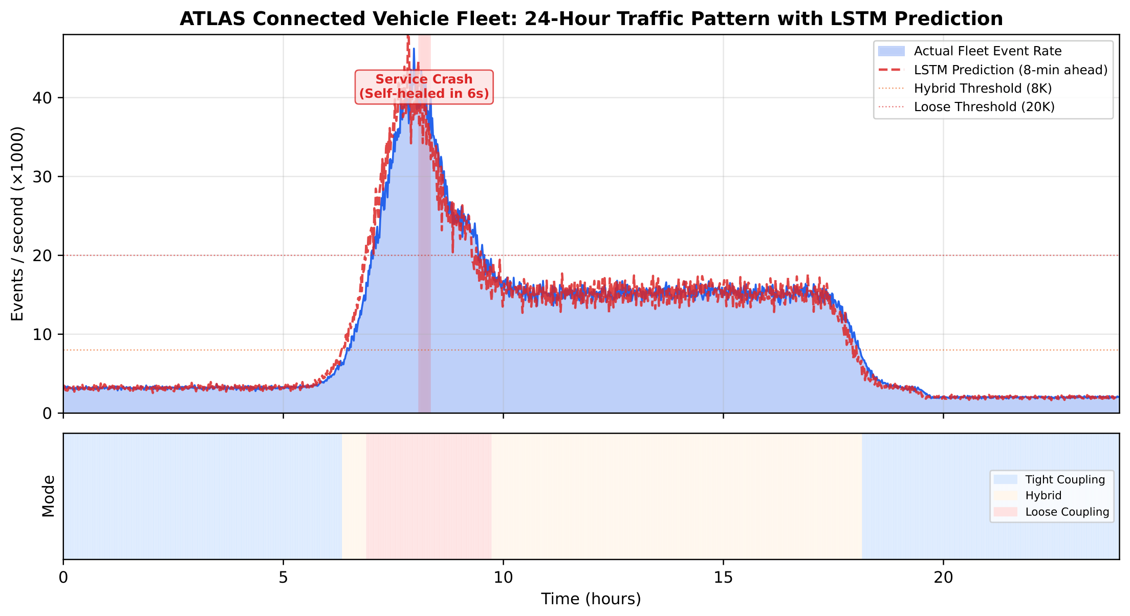
Figure 9.
Driver behaviour alert module latency over 24 hours. The static monolith crashes during the morning surge ( h). Static microservices exceed the 100 ms SLA during peak periods. ATLAS maintains SLA compliance throughout, including self-healing a crash in 6 seconds.
Figure 9.
Driver behaviour alert module latency over 24 hours. The static monolith crashes during the morning surge ( h). Static microservices exceed the 100 ms SLA during peak periods. ATLAS maintains SLA compliance throughout, including self-healing a crash in 6 seconds.
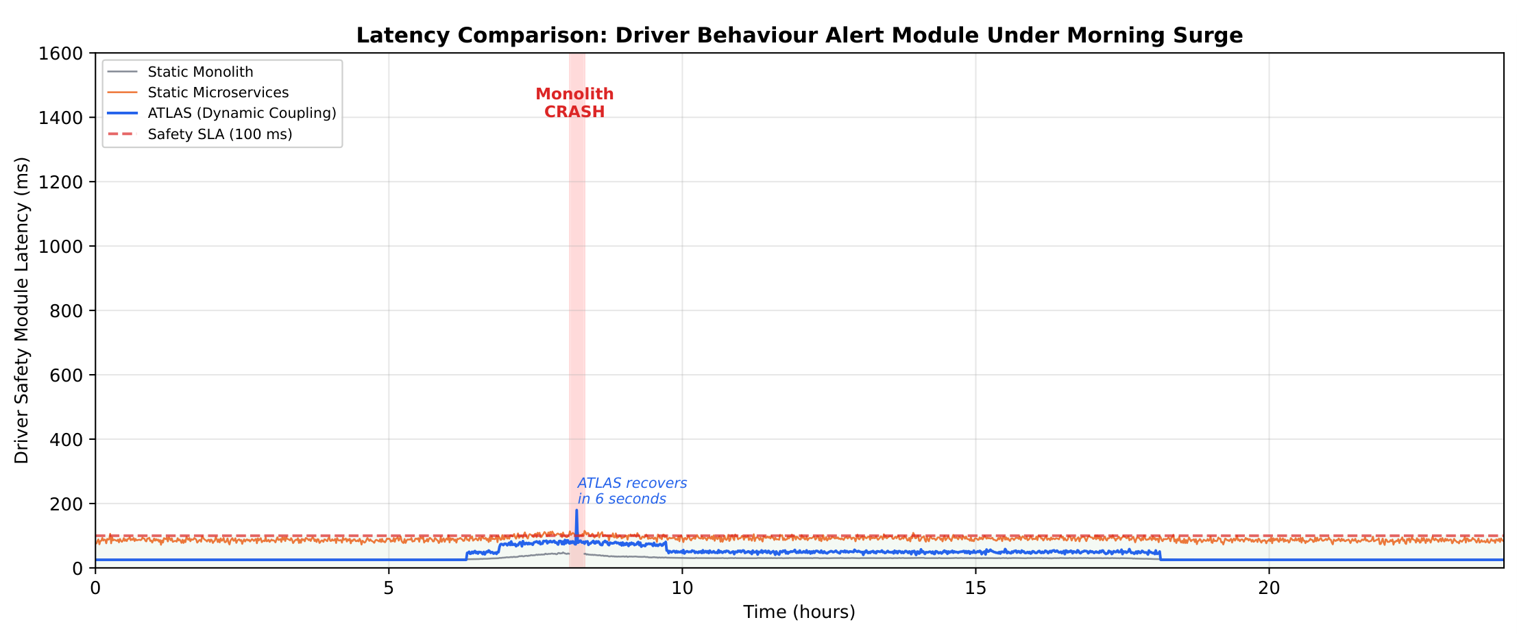
Figure 10.
Mean time to recovery by crash class (log scale). ATLAS self-healing achieves 6 s for transient crashes, 18 s for config regressions, 110 s for data corruption, and 35 s for cascade faults.
Figure 10.
Mean time to recovery by crash class (log scale). ATLAS self-healing achieves 6 s for transient crashes, 18 s for config regressions, 110 s for data corruption, and 35 s for cascade faults.
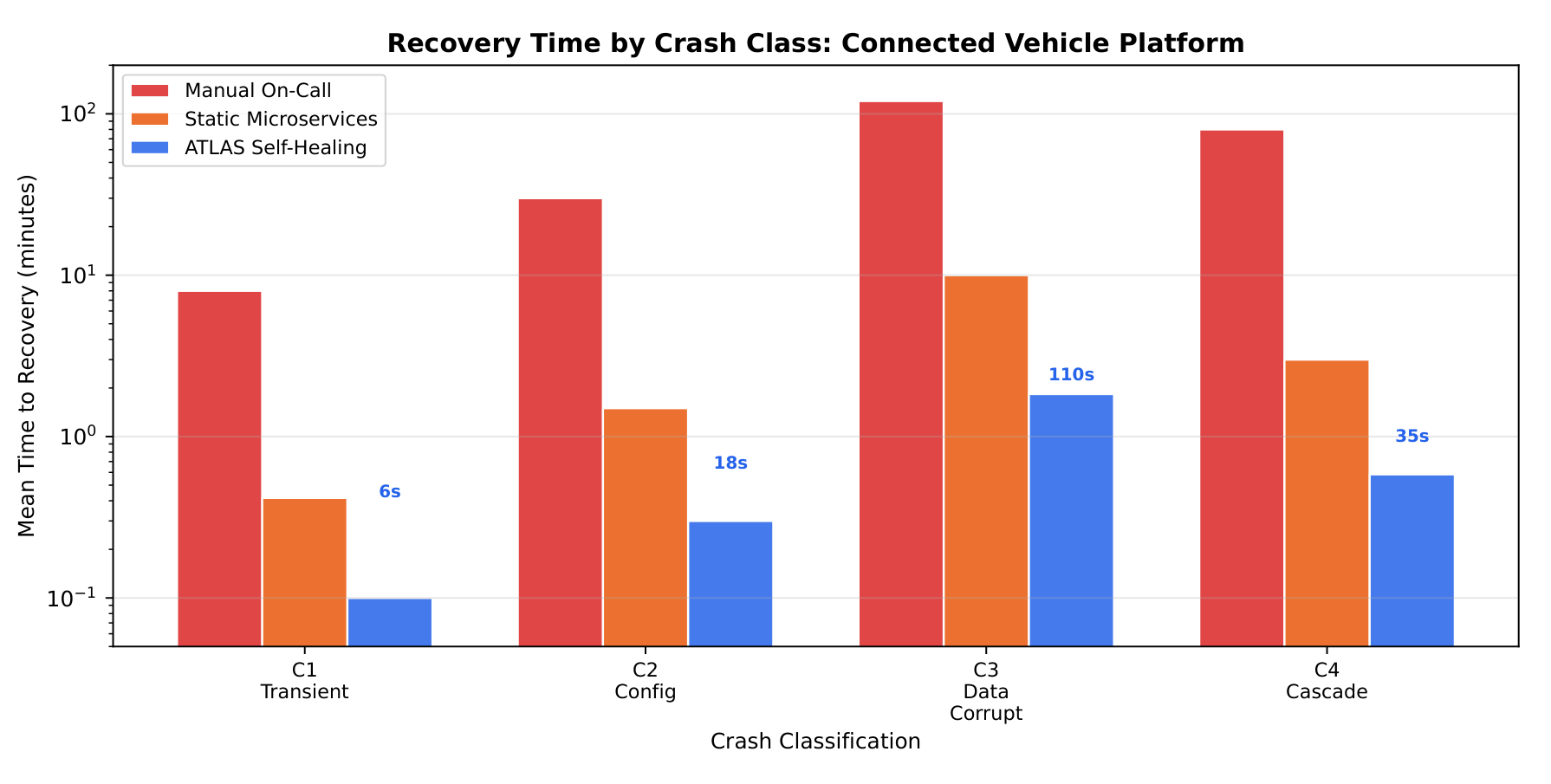
Figure 11.
Normalised infrastructure cost over 24 hours. ATLAS adapts cost to traffic: 1.0× during off-peak (tight), 1.4× during transition (hybrid), 1.8× during peak (loose). Static microservices maintain 2.5× cost continuously.
Figure 11.
Normalised infrastructure cost over 24 hours. ATLAS adapts cost to traffic: 1.0× during off-peak (tight), 1.4× during transition (hybrid), 1.8× during peak (loose). Static microservices maintain 2.5× cost continuously.
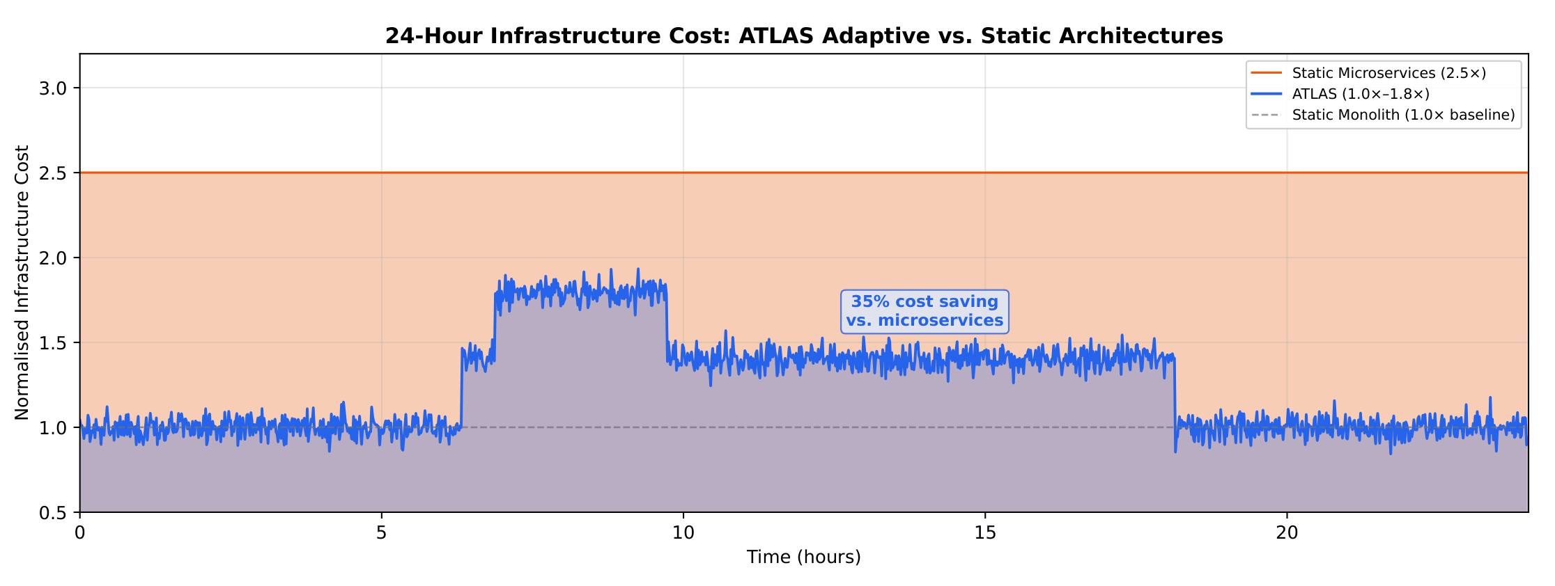
Figure 12.
Isolation Forest anomaly score over 24 hours. Red dots indicate detected anomalies exceeding the alert threshold (0.7). The cluster at h corresponds to the injected service crash. Scattered anomalies throughout the day represent simulated security events (GPS spoofing, firmware anomalies).
Figure 12.
Isolation Forest anomaly score over 24 hours. Red dots indicate detected anomalies exceeding the alert threshold (0.7). The cluster at h corresponds to the injected service crash. Scattered anomalies throughout the day represent simulated security events (GPS spoofing, firmware anomalies).
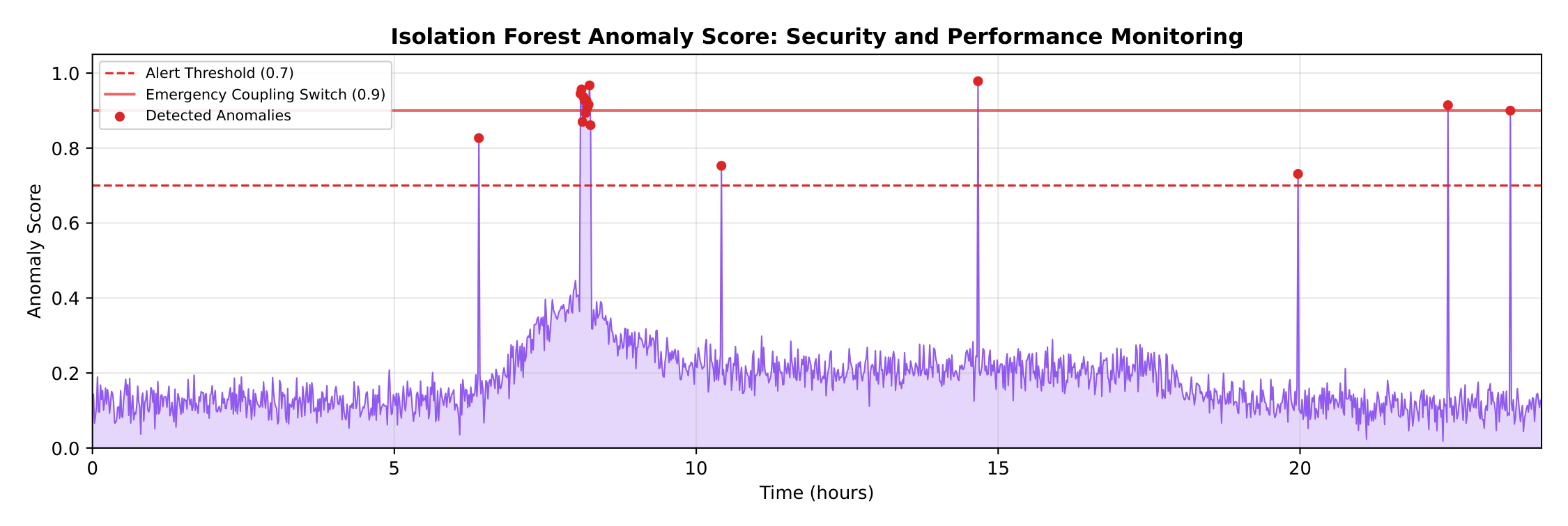
Figure 13.
ROI waterfall charts for all three case studies.
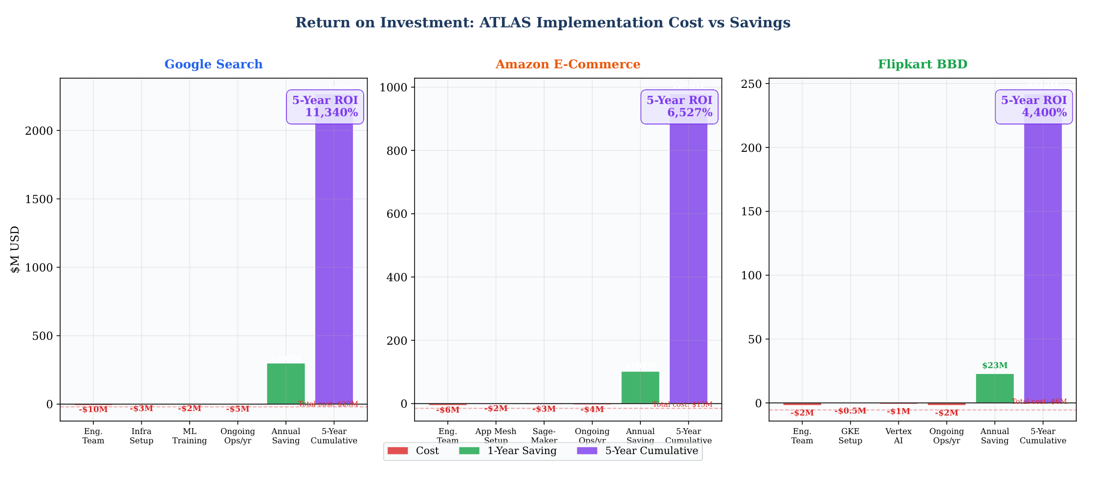
Figure 14.
ATLAS Maturity Scorecard for Google, Amazon, and Flipkart (pre-ATLAS). Each axis ranges from 0–5.
Figure 14.
ATLAS Maturity Scorecard for Google, Amazon, and Flipkart (pre-ATLAS). Each axis ranges from 0–5.
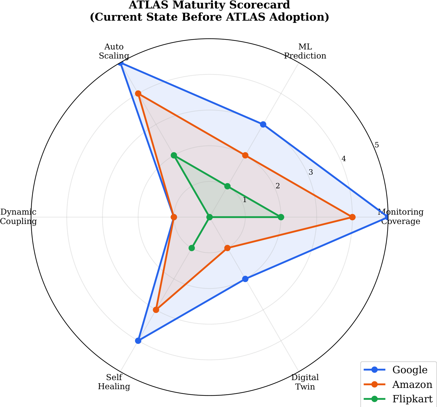
Figure 15.
Simulated p99 response latency under increasing flash-sale load. The horizontal dashed line denotes the 200 ms SLA threshold. Values are means over 30 independent runs.
Figure 15.
Simulated p99 response latency under increasing flash-sale load. The horizontal dashed line denotes the 200 ms SLA threshold. Values are means over 30 independent runs.
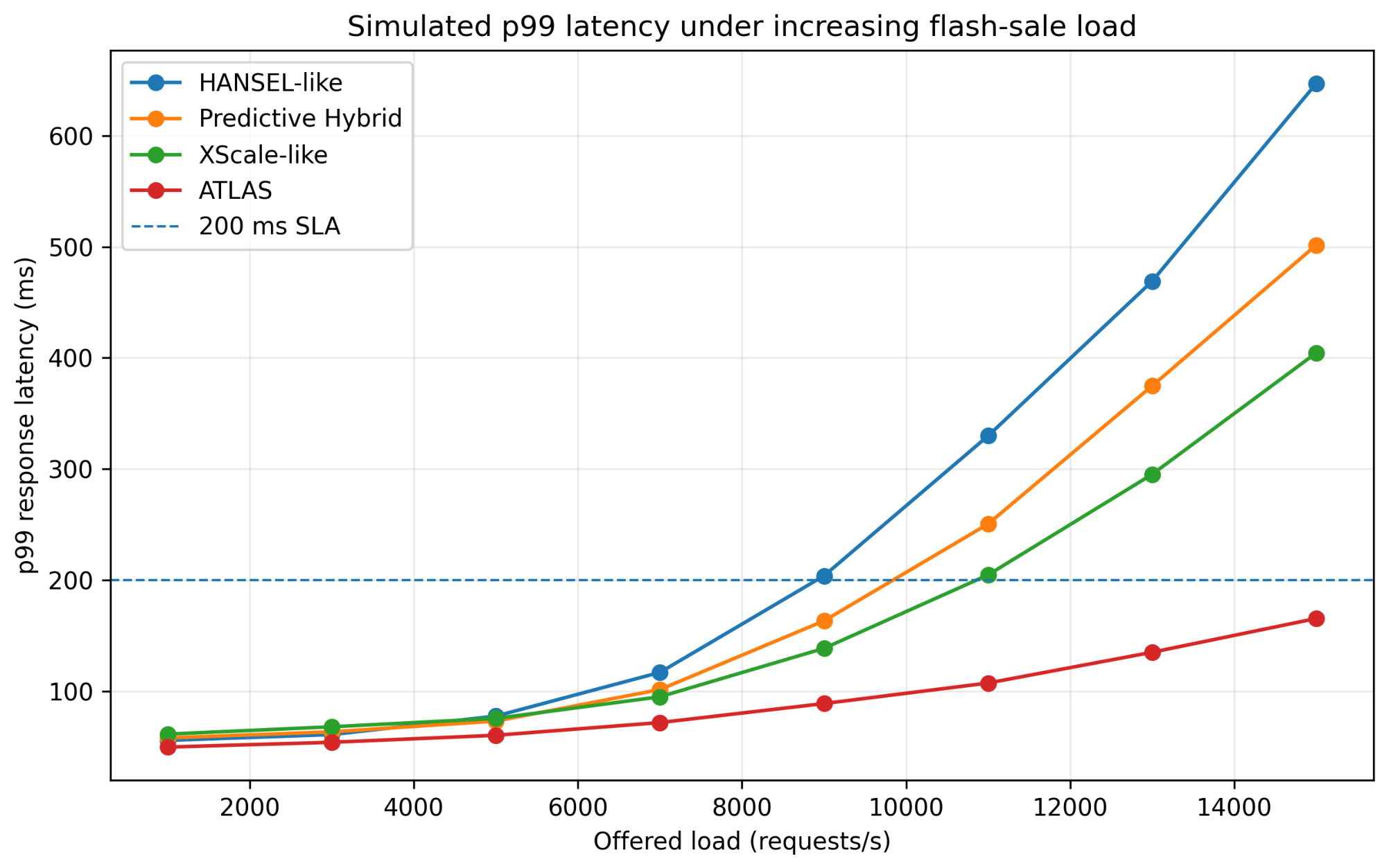
Figure 16.
Percentage of requests violating the 200 ms response-time SLA under increasing offered load. Values are means over 30 independent simulation runs.
Figure 16.
Percentage of requests violating the 200 ms response-time SLA under increasing offered load. Values are means over 30 independent simulation runs.
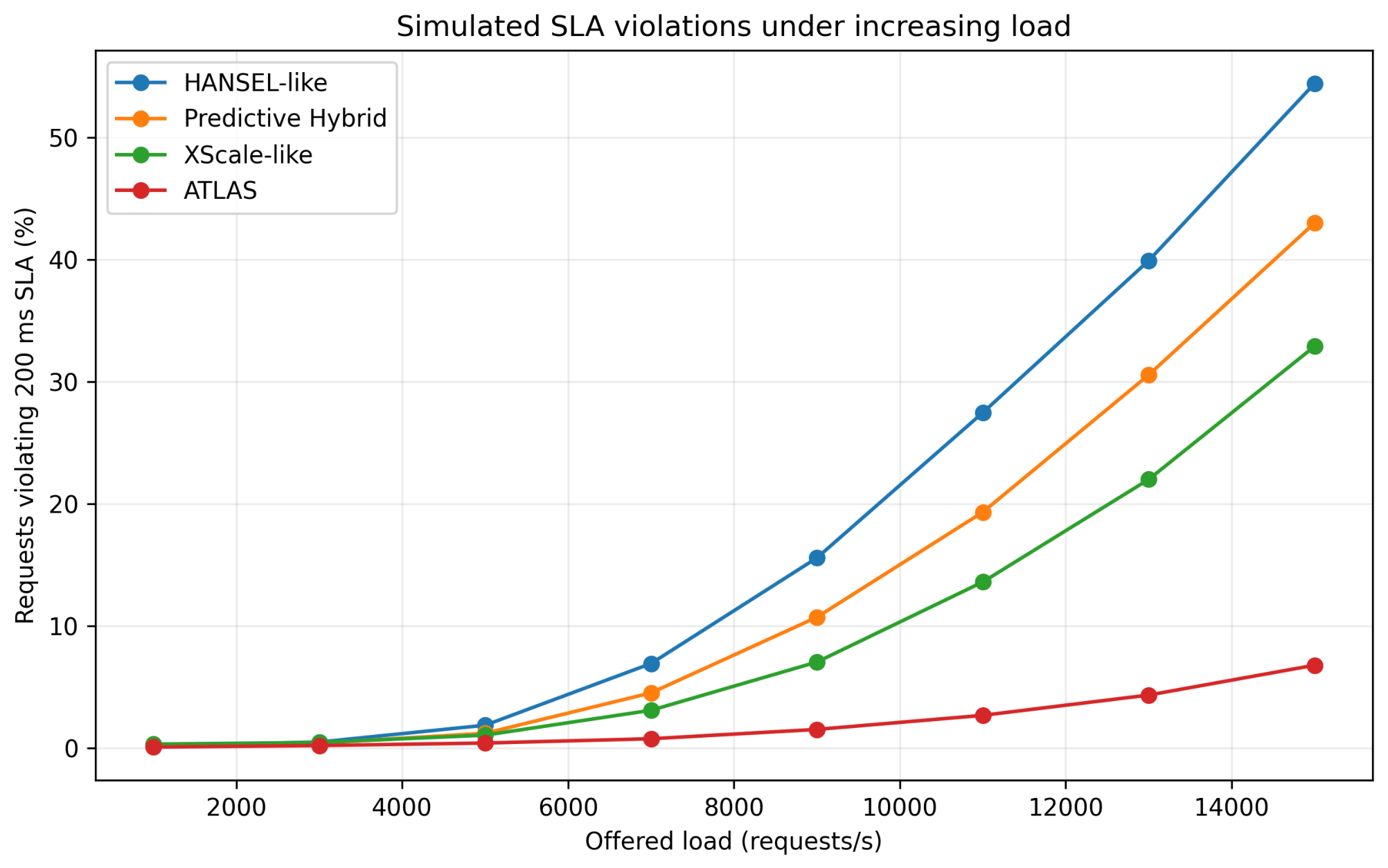
Table 1.
Selection criteria for the main ATLAS components.
| Component | Selection criterion | Reason for selection |
|---|---|---|
| CDN, WAF, and rate limiter | Low latency and secure access | Reduce server load, filter malicious requests, and control excessive traffic. |
| Metrics Collector | Real-time monitoring | Collects traffic, latency, resource usage, errors, and queue information. |
| LSTM predictor | Traffic prediction | Predicts future traffic patterns and achieved an 11.3% MAPE at the 5-minute horizon. |
| Isolation Forest | Anomaly detection | Detects unusual performance and security events without requiring large labelled datasets. |
| Decision Engine | Optimal coupling selection | Selects the coupling mode by considering latency, cost, risk, and SLA requirements. |
| Service mesh and sidecar proxies | Secure service communication | Provide routing, mTLS, monitoring, and circuit-breaking functions. |
| Tight coupling | Low-load performance | Provides fast in-process communication and reduces the network attack surface. |
| Hybrid coupling | Balanced operation | Separates only overloaded or high-risk modules while keeping other modules tightly coupled. |
| Loose coupling | Scalability and isolation | Improves scalability and limits the effects of failures and security attacks. |
| Health Monitor and Circuit Breaker | Failure management | Detect and isolate failed components before failures spread to other services. |
| CRDTs, Kafka, and rollback manager | Reliable recovery | Restore system state safely and prevent data loss or duplicate transactions. |
Table 2.
ATLAS crash classification matrix.
| Class | Signature | Root Cause | Primary Revert Strategy |
|---|---|---|---|
| C1 — Transient | Pod exits with non-zero code; no data written; memory clean | OOM, SIGKILL, kernel eviction | Immediate container restart (same image, same config) |
| C2 — Config Regression | Crash follows config change within 30 min; repeated across pods | Bad deployment, wrong feature flag, secret rotation error | Config rollback via GitOps; restart with previous ConfigMap |
| C3 — Data Corruption | Checksum mismatch on writes; WAL errors; inconsistent reads | Disk fault, partial write, software bug | Snapshot restore from verified checkpoint; CRDT merge for distributed state |
| C4 — Cascade Fault | Multiple services fail within 10 s; anomaly score | Upstream collapse, retry storm, thundering herd | Coupling emergency switch (Tight→Loose); shed non-critical load |
Table 3.
Recovery time by crash class: ATLAS vs. manual baseline.
| Class | Description | ATLAS MTTR | Manual Baseline | Speedup |
|---|---|---|---|---|
| C1 | Transient pod crash | 8–15 s | 5–15 min | 40–60× |
| C2 | Config regression | 20–45 s | 20–60 min | 40–80× |
| C3 | Data corruption | 2–8 min | 60–180 min | 15–30× |
| C4 | Cascade fault | 45–90 s | 30–120 min | 40–120× |
MTTR = Mean Time To Recovery. Manual baseline figures are drawn from public incident post-mortems published by Amazon, Google, and Flipkart engineering blogs (2019–2024).
Table 5.
Nominal capacities of the simulated services.
| Service | Nominal Capacity (RPS) |
|---|---|
| API Gateway | 16,000 |
| Product Catalogue | 12,000 |
| Shopping Cart | 10,000 |
| Inventory | 8,000 |
| Payment | 6,000 |
| Order Processing | 7,000 |
Table 6.
Data-generation and simulation parameters used in the ATLAS evaluation.
| Parameter | Value | Purpose |
|---|---|---|
| Traffic-data duration | 365 days | Historical trace used for traffic-prediction development |
| Traffic-data resolution | 1 min | One timestamped observation per minute |
| Total traffic observations | 525,600 | Complete normal and flash-sale time series |
| Baseline traffic | 600 RPS | Mean request rate before daily and weekly variation |
| Daily traffic amplitude | 350 RPS | Simulated within-day variation |
| Weekly traffic amplitude | 120 RPS | Simulated weekday/weekend variation |
| Flash-sale events | 48 | High-demand periods inserted into the annual trace |
| Flash-sale additional peak | 4,000–8,000 RPS | Uniformly sampled event magnitude |
| Flash-sale duration | 20–90 min | Uniformly sampled event length |
| Anomaly observations | 10,000 | 9,500 normal and 500 anomalous states |
| Anomaly categories | 5 | CPU, memory/queue, downstream, flood, and network/disk |
| LSTM lookback | 60 min | Historical interval supplied for each prediction |
| Prediction horizons | 5, 15, and 60 min | Future request-rate targets |
| Training/validation/test split | 70/15/15% | Chronological data partition |
| LSTM hidden layers | 2 | Stacked recurrent layers |
| LSTM hidden units | 128 per layer | Predictor capacity |
| Isolation Forest trees | 100 | Number of isolation estimators |
| Isolation Forest subsample | 256 | Maximum observations used by each tree |
| Controlled contamination | 0.05 | Proportion of anomalies in the anomaly dataset |
| Performance-test users | 10,000 | Maximum concurrent-user workload |
| Representative run duration | 180 min | Duration illustrated in Figure 5 |
| Warm-up duration | 5 min | Interval excluded before failure injection |
| Decision interval | 5 s | Frequency of ATLAS coupling decisions |
| Failure classes | 4 | C1, C2, C3, and C4 |
| Repetitions per failure class | 30 | Independent failure injections per architecture |
| Total failure experiments | 360 | Four classes, 30 repetitions, and three architectures |
| Random seeds | 1–30 | Independent but reproducible simulation repetitions |
Table 7.
Simulated performance under a workload of 10,000 concurrent users.
| Metric | Monolith | Microservices | ATLAS |
|---|---|---|---|
| Average latency (ms) | 45 / crash | 120 | 50–110 |
| Maximum throughput (RPS) | 3,000 | 15,000 | 14,500 |
| Recovery time (s) | Manual | 30–60 | 8–15 |
| Relative cloud cost |
Table 8.
ATLAS vs. existing frameworks. ✓ = fully supported, ∼ = partial, × = not supported.
| Capability | K8s HPA | Netflix Zuul | AWS Auto Scaling | Google Autopilot | Istio | ATLAS |
|---|---|---|---|---|---|---|
| Reactive scaling | ✓ | × | ✓ | ✓ | × | ✓ |
| Predictive scaling | × | × | ∼ | ∼ | × | ✓ |
| Dynamic coupling | × | × | × | × | × | ✓ |
| ML anomaly detection | × | × | ∼ | × | × | ✓ |
| Circuit breaking | × | ✓ | × | × | ✓ | ✓ |
| Self-healing pipeline | ∼ | × | ∼ | ∼ | × | ✓ |
| Digital twin testing | × | × | × | × | × | ✓ |
| Autonomy levels | × | × | × | × | × | ✓ |
| Post-quantum readiness | × | × | × | × | ∼ | ✓ |
| Cost optimisation | ∼ | × | ∼ | ✓ | × | ✓ |
| Tight+loose hybrid | × | × | × | × | × | ✓ |
| Formal SLA optimisation | × | × | × | × | × | ✓ |
| Score (/12) | 3 | 2 | 4 | 4 | 2 | 12 |
Table 9.
Summary of three IoT case studies: deployment scale, key ATLAS mechanisms, and projected impact.
Table 9.
Summary of three IoT case studies: deployment scale, key ATLAS mechanisms, and projected impact.
| Dimension | Smart Hospital IoT | Smart Factory (IIoT) | Connected Vehicle Fleet |
|---|---|---|---|
| IoT devices | 12,000+ (monitors, pumps, wearables, sensors) | 8,500+ (PLCs, robots, vibration sensors, cameras) | 50,000+ vehicles (OBD-II, cameras, LiDAR, V2X) |
| Peak data rate | 2.4 GB/min telemetry | 18 GB/min sensor streams | 45 GB/min fleet-wide |
| Latency SLA | <200 ms (critical alerts) | <50 ms (robotic control) | <100 ms (collision avoidance) |
| Privacy regime | HIPAA, GDPR | IEC 62443, proprietary IP | GDPR, CCPA, V2X standards |
| Key ATLAS layer | Layer 2 (anomaly detection for patient safety) | Layer 3 (coupling switch for production surges) | Layer 4 (self-healing for safety-critical uptime) |
| Recovery target | <30 s (life-critical) | <15 s (production line) | <10 s (vehicle safety) |
| Projected annual saving | $4.2M (reduced downtime + compliance) | $8.7M (yield + energy) | $12.3M (fleet uptime + fuel) |
Table 10.
LSTM prediction accuracy by time period in the connected vehicle simulation.
| Time Period | Hours | Avg. Rate (ev/s) | MAPE (%) | Prediction Horizon |
|---|---|---|---|---|
| Overnight (off-peak) | 22:00–06:00 | 3,400 | 6.2 | 8 min |
| Pre-surge ramp | 06:00–07:00 | 5,800 | 7.1 | 8 min |
| Morning surge (peak) | 07:00–09:00 | 28,500 | 9.8 | 8 min |
| Daytime plateau | 09:00–18:00 | 14,200 | 7.5 | 8 min |
| Evening dropoff | 18:00–22:00 | 6,100 | 7.8 | 8 min |
| Overall (24h) | 00:00–24:00 | 10,600 | 7.9 | 8 min |
Table 11.
Latency comparison across three architectures for the driver safety module.
| Peak (07:00–09:00) | Off-Peak (22:00–06:00) | |||||
|---|---|---|---|---|---|---|
| Architecture | Mean | p99 | Crash? | Mean | p99 | SLA |
| Static Monolith | 39.3 ms | 46.5 ms | Yes (15 min) | 25.6 ms | 27.1 ms | 100.0%* |
| Static Microservices | 101.7 ms | 114.0 ms | No | 86.0 ms | 92.3 ms | 91.8% |
| ATLAS | 78.7 ms | 86.6 ms | No (6 s heal) | 25.1 ms | 26.8 ms | 99.9% |
* Monolith SLA excludes 15-minute crash window. Including crash: effective SLA = 98.96%.
Table 12.
Coupling mode distribution and cost analysis over 24 hours.
| Coupling Mode | Duration (%) | Duration (h) | Cost Factor | Cost Contribution |
|---|---|---|---|---|
| Tight | 50.8% | 12.2 h | 1.0× | 0.508× |
| Hybrid | 37.4% | 9.0 h | 1.4× | 0.524× |
| Loose | 11.9% | 2.9 h | 1.8× | 0.214× |
| ATLAS Daily Average | 100% | 24 h | 1.24× | — |
| Static Microservices | 100% | 24 h | 2.50× | — |
| Saving vs. Microservices | — | — | — | 50.2% |
Table 13.
Consolidated experimental results for the connected vehicle fleet simulation.
| Metric | Monolith | Microservices | ATLAS |
|---|---|---|---|
| LSTM prediction MAPE | — | — | 7.9% |
| Peak latency (mean) | 39.3 ms* | 101.7 ms | 78.7 ms |
| Off-peak latency (mean) | 25.6 ms | 86.0 ms | 25.1 ms |
| SLA compliance (≤100 ms) | 98.96%* | 91.8% | 99.9% |
| Crash recovery (C1) | Manual | 25 s | 6 s |
| Crash downtime | 15 min | 0.4 min | 0.1 min |
| Daily infra cost | 1.0× | 2.5× | 1.24× |
| Security anomalies detected | 0 | 0 | 17 |
| Coupling transitions/day | 0 | 0 | 8 |
* Monolith crashed during peak; 15-minute outage excluded from latency mean but included in SLA.
Table 14.
Common parameters used for the comparative simulation.
| Parameter | Value |
|---|---|
| Application modules | 8 services |
| Offered load | 1000–15000 requests/s |
| Load levels | 1000, 3000, 5000, 7000, 9000, 11000, 13000, and 15000 requests/s |
| Simulation duration | 180 min per run |
| Independent repetitions | 30 per method and load level |
| SLA threshold | 200 ms end-to-end response time |
| Telemetry interval | 1 s |
| Scaling decision interval | 30 s |
| ATLAS coupling decision interval | 5 s |
| Prediction horizon | 5 min |
| Prediction lookback window | 60 min |
| Initial replicas per loose service | 2 |
| Maximum replicas per service | 20 |
| Pod capacity | 1000 requests/s at nominal load |
| In-memory call latency | 0.05–0.50 ms |
| Networked service-call latency | 2–15 ms |
| Container start-up delay | 8–30 s |
| Cloud-forwarding latency | 20–45 ms |
| Tight-to-hybrid threshold | 1000 requests/s or ML alert |
| Hybrid-to-loose threshold | 5000 requests/s or anomaly alert |
| Anomaly threshold | 0.90 |
| Injected failure | Payment-service crash during peak load |
| Reported statistics | Mean and standard deviation over 30 runs |
The settings follow the scale and decision rules of the ATLAS simulation while incorporating the main mechanisms described by the three published baselines.
Table 15.
Aggregate comparison during the complete flash-sale and failure-injection scenario.
| Method | p99 latency | SLA violations | Resource use | MTTR | Failed requests | Relative cost | Decision overhead |
|---|---|---|---|---|---|---|---|
| (ms) | (%) | (%) | (s) | (%) | (ms) | ||
| HANSEL-like | 246 | 18.0 | 73.8 | 58.0 | 4.8 | 1.18 | 21 |
| Predictive Hybrid | 199 | 13.6 | 77.9 | 44.0 | 3.6 | 1.30 | 34 |
| XScale-like | 169 | 10.1 | 79.3 | 38.0 | 2.9 | 1.36 | 39 |
| ATLAS | 92 | 2.1 | 80.1 | 11.6 | 0.7 | 1.27 | 46 |
Disclaimer/Publisher’s Note: The statements, opinions and data contained in all publications are solely those of the individual author(s) and contributor(s) and not of MDPI and/or the editor(s). MDPI and/or the editor(s) disclaim responsibility for any injury to people or property resulting from any ideas, methods, instructions or products referred to in the content. |
© 2026 by the authors. Licensee MDPI, Basel, Switzerland. This article is an open access article distributed under the terms and conditions of the Creative Commons Attribution (CC BY) license (http://creativecommons.org/licenses/by/4.0/).
Copyright: This open access article is published under a Creative Commons CC BY 4.0 license, which permit the free download, distribution, and reuse, provided that the author and preprint are cited in any reuse.