
Submitted:
12 March 2026
Posted:
17 March 2026
You are already at the latest version
Abstract
Draft pick value charts are widely used by NFL teams to evaluate trade proposals during the draft. Traditional charts provide point estimates for the relative value of each selection but do not quantify the uncertainty associated with those values. This paper introduces a statistical framework for estimating the uncertainty in draft pick values using historical trade data. Starting from the Rich Hill draft chart as a prior mean valuation, deviations between observed trade outcomes and chart values are analyzed to estimate the variability associated with each pick. Because individual picks have limited observations, a correlation structure between neighboring selections is introduced through a custom kernel function. Kernel regression is then applied to produce smooth and stable estimates of the standard deviation associated with each pick. The proposed framework also allows for an empirical comparison between widely used draft value charts. Using historical trade data, the Rich Hill chart is shown to provide a better baseline representation of observed trade behavior than the traditional Jimmy Johnson chart. The resulting model provides probabilistic confidence intervals for draft pick values and enables the evaluation of trades in terms of statistical percentiles. Model calibration is assessed using normalized residuals, log-likelihood, and confidence interval coverage. The results demonstrate that the proposed approach produces well-calibrated uncertainty estimates while preserving the empirical structure of draft trades.
Keywords:
draft pick valuation
; uncertainty quantification
; kernel regression
; correlation structure
1. Introduction
As soon as the Super Bowl ends each year, attention across the football world shifts to free agency and the NFL Draft. Media and fans begin projecting trades, often relying on publicly available trade charts as reference. Beyond the public gaze, each team uses its own trade chart.
The Jimmy Johnson trade chart was created in the 1990s to provide a simple “currency” for valuing draft picks consistently across teams, and it quickly became widely adopted. Over the years, changes in the league, such as the creation of compensatory picks (1993), the introduction of the current CBA (2011), and the ability to trade those picks (2024), have pushed teams to update their charts.
At least four major documented attempts [1] have been made to analyze past trades and determine the “true” value of each draft pick, most notably by Rich Hill [2]. Each team has certainly modified, improved, or perhaps even fully replaced the classic Jimmy Johnson chart. However, according to former Patriots head coach Bill Belichick, all teams remain “more or less on the same page” [3] when it comes to the value of draft picks.
The appearance of different models raises the question: is the Jimmy Johnson chart truly outdated? The Open Trade Project is the result of that enterprise. Unlike the charts from Jimmy Johnson and Rich Hill, which assign a single value to each pick, our model explicitly quantifies uncertainty. In simple terms, rather than identifying a single “bullseye” value for each pick, we examine the distribution of values around that point, using data from past trades.
This paper begins with a simple model that can be used to evaluate the “transacted value” of each pick in a trade. That model is then applied to assess the performance of the Jimmy Johnson and Rich Hill charts from 2012 to 2025, identifying the Rich Hill chart as a significant improvement. Finally, we develop a statistical model to quantify the uncertainty in the value of each pick, extending the analysis of trades from a binary “winner or loser” framework to one expressed in terms of percentile outcomes.
In this paper, an effort is made to use non-technical language wherever possible, anticipating that many readers will be football enthusiasts or members of the media. However, full scientific rigor is necessary; therefore, the authors attempt to guide the non-technical audience through the essential portions of the text without compromising understanding.
2. Proposing a Model to Evaluate Every Trade
It is appropriate to begin with the usual procedure for proposing or evaluating a trade. Our model will be developed using the trade between the Tennessee Titans and the Seattle Seahawks in the 2025 NFL Draft (Table 1) as an example. Based on the Jimmy Johnson chart, the Titans gave up 550 points and received 560 points, and therefore “won” the trade by 10 points. Using the Rich Hill chart instead, the Titans “lost” the trade by 7 points.1
This example clearly illustrates that the Jimmy Johnson and Rich Hill charts result in different outcomes depending on the picks involved. Prior to proposing any modifications or improvements, it is convenient to evaluate and compare the performance of the two models. That investigation is carried out in the next section. Also, it is worth mentioning that the numerical scales of the Jimmy Johnson and Rich Hill charts are not directly comparable: they represent different arbitrary currencies.
2.1. Dataset assumptions
In order to evaluate past trades systematically, we need a consistent model to process each transaction. Before constructing such model, several assumptions are made to narrow and standardize the dataset:
- No trades involving players are considered; the dataset consists exclusively of pick-for-pick swaps.
- No trades involving future picks are considered.
- The complete dataset includes trades from 2002 (the year of the most recent NFL expansion) through 2025.
- Compensatory picks (including Resolution JC-2A) are treated as regular picks.
- No round distinctions are made. For example, the last pick of the first round is labeled #32 and the first pick of the second round is labeled #33. This ensures consistency across drafts, especially given that the number of compensatory picks varies from year to year.
- Individual exceptions (such as forfeited picks) are treated as “ghost” selections.2
- This analysis does not attempt to evaluate players or post-draft player success; only the valuation of picks and trades is modeled.
2.2. Trade Parity Model - A Prelude to Evaluating the Jimmy Johnson and Rich Hill Charts
We proceed to develop the model used to analyze individual trades. Each trade consists of a transaction, and the goods being transacted are draft picks. The idea behind trade charts (or any mathematical model, in that regard) is to create a currency to evaluate those transactions. Evaluation of a trade using the Jimmy Johnson or Rich Hill charts mostly results in a clear winner (for example, Table 1). Trades are rarely even, i.e., the picks transacted by both teams rarely amount to equal values. This is actually expected if the model describes each pick as a rigid value.
Our approach is fundamentally different. Rather than treating picks as fixed, rigid values, we decompose the value of each individual pick into two components:
- The first component is the “prior” or expected value. We assume this value is supplied by whichever trade chart is being used. For pick n, this is denoted by .
- The second component represents the uncertainty, fluctuation, or deviation. This term allows us to incorporate external factors that may influence each trade. For pick n, this is denoted by .
The idea behind separating expected value and uncertainty is best illustrated through the evaluation of the trade shown in Table 1:
Where the symbol ⇔ indicates a “transaction", the left side relates to pick 35 and the right side relates to the combination of picks 52 and 82.
The choice of trade chart determines the value of for each pick. The uncertainty terms are not known a priori. Introducing uncertainty allows us to make the central assumption of our model: that all trades are exact. In other words, each team gives and receives picks whose true total values are equal, even though those values may differ from their expected values due to uncertainty. Under this assumption, each trade becomes an equality, which we call the value equation:
The model and the assumption of exact trades are independent of the choice of trade chart. The next step is to determine the uncertainty associated with each pick. To illustrate, consider again the trade in Table 1 using the Jimmy Johnson chart. The Titans surrendered two picks, worth 560 points in total, and received a single pick worth 550 points. Substituting the appropriate values into Equation 2 gives
Where values are in Jimmy Johnson points. This may be rewritten as
In our model, since trades are exact, the terms “loss” and “profit” do not apply. Our goal is simply to determine the uncertainty associated with each pick. Mathematically, in this example we have one equation with three unknowns, so additional assumptions are required to obtain a solution. Our next assumption is straightforward: the uncertainty value for each pick is proportional to its prior value. To illustrate the feasibility of this assumption, we propose an example solution which satisfies Equation 4:

Table 2.
Example solution for pick uncertainty (), for the trade shown in Table 1.
Table 2.
Example solution for pick uncertainty (), for the trade shown in Table 1.
| Pick number (n) | Mean value () | Uncertainty () | Uncertainty (% of ) |
|---|---|---|---|
| 35 | 550 | 30 | 5.45% |
| 52 | 380 | 5 | 1.31% |
| 82 | 180 | 15 | 8.33% |
Does it make sense that the absolute uncertainty of pick 82 is greater than that of pick 52, even if pick 52 is expected to be worth more points than pick 82? Not really. The inconsistency of that solution is also clear when we evaluate the uncertainties as percentages of prior values. In our case, the uncertainty for pick 82 is 8% of its expected value, while the uncertainties for picks 35 and 52 fall at 5% and below 2% of the respective prior values.
By enforcing proportionality, we guarantee that the total uncertainty is distributed fairly across all picks involved. Mathematically, this results in
Here, absolute values are used to ensure that the uncertainties entering the proportionality relationships are positive. For example, from Equation 3 we see that, since the Seahawks lost the trade, the uncertainty terms for the picks sent by Seattle ( and ) are negative. Conversely, the profit in the transaction, experienced by Tennessee, is attributed entirely to pick 35, so is positive. Although we have noted that, under the assumption of exact trades, the notions of “loss” and “profit” are not meaningful in a strict sense, the winner–loser identification still determines the signs of the uncertainty terms.
A direct consequence of the proportionality assumption is that the actual transaction value must lie between the prior values of the picks sent and received. Substituting prior values into Equation 5 results in
The combination of the value equation and the proportionality equations (6) results in a system with three equations and three unknowns. Solving these equations simultaneously produces the uncertainty values shown in Table 3.
As expected, the calculated uncertainty values for picks 52 and 82 are negative, and the uncertainty for pick 35 is positive. The transacted value for each pick is reconstructed using the calculated uncertainties and the prior means. According to the two assumptions, pick 35 transacted for 554.95 points (instead of the 550 points predicted by the Jimmy Johnson chart). The combination of picks 52 and 82 transacted for exactly the same value.
Tennessee sent pick 35, originally valued at 550 points, and received 554.95 points in return. Likewise, Seattle sent picks 52 and 82 (valued at 560 points) and received 554.95 points in return. The ratio between absolute uncertainty and prior value for each pick is the same, demonstrating the application of the proportionality assumption (in contrast to Table 2).
In subsequent sections, these uncertainty terms are treated as realizations of symmetric random deviations around zero. This reflects the assumption that trades do not systematically over- or under-value picks on average.
2.3. Generalization of the Trade Parity Model
The non-technical reader may skip to the next section without any loss of understanding.
The trade parity model is now generalized to account for transactions involving any number of picks. The generalized value equation is
where S is the set of picks sent (i picks) and R is the set of picks received (j picks). The generalized proportionality equations are
Absolute values are included for generality; the algorithm that implements the model determines which uncertainty values are positive and which are negative. By construction, this system of equations always has a unique solution.
Each trade produces equations, and solving the resulting linear system yields individual uncertainty values, one for each pick involved in the transaction. From this point forward, no additional reference will be made to “winner”, “loser”, “profit”, or “loss”.
3. Evaluation of the Jimmy Johnson and Rich Hill Charts
To accurately compare the Jimmy Johnson and Rich Hill charts, we must select an appropriate subset of our dataset. The Jimmy Johnson chart was developed in the 1990s, whereas the Rich Hill chart was first made public in 2017 and was designed specifically to reflect changes introduced by the 2011 CBA.
Our trade parity model was applied to both the Jimmy Johnson and Rich Hill charts, using draft trades from 2012–2025 (post–2011 CBA). A total of 318 trades resulted in 1101 uncertainty observations for individual picks. The reconstructed transacted values are shown in Figure 1 (Jimmy Johnson) and Figure 2 (Rich Hill).
Visual inspection suggests that the dispersion of picks around the expected mean is greater in the Jimmy Johnson chart (i.e., the vertical spread of values for individual picks is larger). In Figure 2, the observations cluster more tightly around the mean values. This suggests that the Rich Hill model provides a better fit.
However, it must be noted that the scales of the two charts are not equal. In the Jimmy Johnson chart, the maximum pick is worth 3000 points, whereas in the Rich Hill chart it is worth 1000 points (also, as noted previously, the “points" in the Jimmy Johnson and Rich Hill charts are two entirely different currencies). As a result, direct visual comparison of the plots may be misleading.
To enable a meaningful comparison between the two charts, a scale-invariant error metric is required. Direct measures such as the root mean square error (RMSE) depend on the magnitude of the underlying scale and therefore cannot be used to compare models expressed in different units. A normalized metric is therefore necessary to evaluate how well each chart represents the empirical trade data.
The RRMSE relative root mean square error is a variation of the common RMSE, where residuals are normalized (allowing comparison between models of different scales, such as the Jimmy Johnson and Rich Hill charts). It represents the “dispersion" of observations around the projected mean and shows how well the model describes the empirical observations. First, the RRMSE can be calculated for each pick in each chart – allowing direct comparison between the same pick in both charts.
The discussion presented in this section is highly relevant to our audience; however, the non–technical readers may skip the equations for RRMSE without loss of understanding.
The RRMSE for pick j is given by
where
- j is the draft pick number,
- is the number of observations involving pick j,
- is the transacted value of pick j in observation i,
- is the mean value predicted by the trade value model for pick j (prior mean),
- is the relative error of the model for that observation.
The RRMSE values for each pick are shown in Figure 3. RRMSE is consistent not only across the two charts but also across different picks within the same chart. For example, the Jimmy Johnson chart produces high dispersion for many late-round picks, indicating that it describes late-round trades less accurately than early– and mid–round trades.
A similar trend appears in the Rich Hill chart: picks in the later rounds also exhibit higher dispersion. However, compared with the Jimmy Johnson chart, the Rich Hill chart reduces the spread of late–round observations around their prior means, even though late–round picks still display greater variability. Overall, the Rich Hill chart resulted in smaller RRMSE for 167 picks (out of 261 total).
The RRMSE analysis may be extended to simultaneous observations of all picks:
where
- P is the total number of draft picks considered,
- is the number of observations involving pick j,
- is the total number of observations,
- is the observed value of pick j in observation i,
- is the mean value predicted by the trade value model (prior mean).
The Rich Hill chart results in a global RRMSE value of 1.6125, compared to 3.9984 for the Jimmy Johnson chart. These results confirm the visual interpretation suggested in Figure 3 is correct: the Rich Hill chart significantly outperforms the Jimmy Johnson chart for trades from 2012–2025, considering not only individual picks but the entire distribution of observations across all picks.
3.1. Improving the Rich Hill Chart: Toward Quantifying Uncertainty in Draft Picks
Up to this point, this paper has focused on evaluating existing trade charts. The Rich Hill chart is widely regarded as a substantial improvement over the Jimmy Johnson chart, despite the absence of any detailed public study directly comparing the two. Our model fills that gap in the literature and provides clear evidence of the Rich Hill chart’s superiority.
Although no public information exists regarding how the Rich Hill chart was constructed, it does provide a better explanation of past trades. This naturally leads to the following question: Is it possible to further improve the Rich Hill chart?
The answer to that question is directly connected to our analysis of RRMSE values. A better model produces smaller errors, both for individual picks and in the aggregate. This has already been achieved by the Rich Hill chart. A perfect model, by contrast, would produce no error at all—meaning that every observation would be perfectly explained by the prior, with all uncertainty terms equal to zero. Improving the Rich Hill chart, in the same way that Rich Hill improved upon the Jimmy Johnson chart, consists of finding a chart that yields even smaller errors.
However, since no model is perfect, observations for each pick will always exhibit some spread around the prior mean. We accept this fact and propose a different type of improvement: instead of attempting to eliminate the error, we embrace it. In practical terms, this means:
- Accepting the Rich Hill chart as a strong baseline;
- Quantifying the uncertainty, i.e., estimating the spread of observations around the prior values with sufficient statistical confidence.
This is precisely what was emphasized in the introduction: rather than searching for a new bullseye, we focus on the spread of observations around the accepted bullseye (the Rich Hill chart).
3.2. Are NFL Draft Trades a Zero–Sum Game?
Initially, our assumption of exact trades implies that the buyer and seller teams receive exactly the same value, even though each individual pick may not transact for its nominal (prior) value. Once again, it does not make sense to evaluate trades in the traditional manner — for example, to say “The Titans won the trade by 10 points” (see Table 1).
Instead, if our approach is successful, we will obtain a distribution for the value of each pick. This will allow us to convert individual observations into statements such as “The selling team received a 76th percentile value for pick 34.” These percentile–based statements, in turn, should enable us to construct a fair grading scale – one that captures trades that are favorable (or unfavorable) for either team without relying on the traditional zero–sum interpretation.
4. Uncertainty Quantification of Draft Picks
Although draft value charts are widely used in practice, relatively little academic work has examined the statistical uncertainty associated with draft pick valuations. Existing studies typically focus on expected value estimation or trade fairness metrics rather than the probabilistic dispersion of pick values. The present work contributes to this literature by explicitly modeling the uncertainty structure of draft pick values using a correlation–based framework.
We now proceed to investigate the uncertainty in the value of each pick. The starting point is the Rich Hill chart; its values (or prior values) are taken as true. Our empirical (trade) observations then serve as the basis for estimating the uncertainty associated with each pick. At first glance, the most straightforward idea would be to treat these observations as samples for each pick and compute a Standard error (SE).
It is important to emphasize that the reconstructed deviations, , are not direct empirical observations. Instead, they are values inferred by solving the trade parity model under the assumption that trades represent approximately rational exchanges between teams. Consequently, the statistical analysis in this section evaluates the internal consistency of the model and the trade charts with the historical trade dataset. In other words, the deviations should be interpreted as model–implied observations rather than raw empirical measurements.
Obtaining independent observations for individual draft picks is inherently difficult. In a typical NFL draft, teams select approximately once per round, meaning that nearby picks rarely appear together in the same trade. As a result, the deviation associated with a given pick is often inferred indirectly from the structure of the trade rather than observed in isolation. This structural property of the draft introduces strong dependence between neighboring picks and further motivates the use of a correlation–based modeling framework.
When we consider the number of picks (261) and the total number of observations (1101), a secondary problem is evident: most picks have very few observations, and several picks have none at all. Standard error estimates are unreliable for such small sample sizes and become reasonably stable only when the number of observations is sufficiently large (commonly on the order of 20–30 per pick), due to the behavior of the sampling distribution of the mean [4].
Additionally, estimating the standard error for individual picks fails to account for the correlation between picks. It is reasonable to assume, for example, that the observations for pick 15 are significantly influenced by those for pick 14, and less influenced by those for, say, pick 20. However, the very existence of correlation between picks actually helps us: despite the limited number of observations, it is still possible to accurately estimate the uncertainty for each pick, provided that we can obtain a good estimate of that correlation.
4.1. Prior Correlation Structure
Starting from the base assumption that neighboring picks are correlated, we proceed to define a correlation structure. This process requires substantial football intuition; in particular, the structure must satisfy some intuitive principles:
- A pick is most strongly correlated with its immediate neighbors, and the influence of other picks decreases as their distance from the original pick increases. For example, pick 7 is more influenced by pick 6 than by pick 10.
- Because the value of draft picks declines sharply with increasing pick number, early picks are more distinct than later picks. Consequently, only a small number of neighboring picks should meaningfully influence the value of pick 7.
- In contrast, the difference between early and late selections within the seventh round is relatively small. Late–round picks are therefore influenced by a larger number of neighboring picks, and they are also more strongly influenced by those neighbors.
The non–technical reader may skip to section “Illustrating the correlation structure" without any loss of understanding.
We define the correlation between two draft picks i and j using a modified squared–exponential function [5] with a variable length scale [6]. This function resembles the standard squared–exponential kernel used in Gaussian processes:
where the length scale grows exponentially with the pick index:
and the parameters are defined as follows:
- are the pick indices,
- is the base length scale for early picks,
- is a scaling factor that controls the exponential growth of the length scale,
- N is the total number of picks (261).
This kernel produces correlations between 0 and 1; in that sense, it behaves similarly to the Pearson correlation coefficient. The parameters and are free hyperparameters and may be optimized or chosen based on domain intuition. In this study, we set and .
A heatmap illustrating the resulting correlation structure is shown in Figure 4. The correlation kernel is symmetric, i.e., the effect of pick i on pick j is equal to the effect of pick j on pick i. The correlation matrix is 261 by 261.
The kernel function defines the prior correlation structure between the deviations () associated with each pick. In other words, it encodes the assumption that deviations in the transacted value of nearby picks tend to move together. If pick i exhibits unusually high or low realized value relative to the Rich Hill chart, neighboring picks are expected to show similar behavior, with the strength of this relationship decreasing as the distance between picks increases.
4.2. Illustrating the Correlation Structure
Some examples illustrate that the correlation function indeed satisfies the principles outlined earlier:
- The correlation between picks 1 and 3 is 0.14, while the correlation between picks 1 and 5 is less than 0.01. This reflects that pick 1 is only meaningfully influenced by a few of its neighbors (picks 2, 3, and 4).
- The correlation between picks 40 and 42 is 0.55, whereas the correlation between picks 40 and 44 is around 0.1. This shows that immediate neighbors exert a stronger influence as the pick number increases, and that a larger set of nearby picks affects the value of the base pick.
- The correlation between picks 220 and 250 is 0.71, and the correlation between picks 249 and 250 exceeds 0.99. This demonstrates that late–round picks are strongly affected by many nearby selections (even those in adjacent rounds) and that neighboring picks become increasingly less distinguishable in terms of value.
4.3. Distributional Assumptions
Let denote the observed transacted value associated with pick i, and let denote the value predicted by the Rich Hill draft chart. The deviation is defined as
Because the Rich Hill values are treated as fixed prior means, the deviations capture the randomness in realized trade values.
We adopt the working assumption that the vector of deviations
follows a multivariate normal distribution
where is the covariance matrix. The covariance matrix is parameterized as
where is the correlation kernel defined in Equation 11, and represents the standard deviation associated with pick i.
This assumption should be interpreted as a modeling approximation rather than a strict claim about the true distribution of trade values. The multivariate normal model is adopted because it provides a tractable probabilistic framework with well–understood properties for constructing confidence intervals and evaluating model calibration.
4.4. Estimation of Standard Errors
We wish to determine the standard deviation for each pick, despite the limited number of observations. The kernel function introduces correlation between picks, effectively increasing the amount of information available for each pick by borrowing strength from its neighbors.
Although standard error estimates for picks with few observations are not highly accurate, they are still useful as initial estimates. These preliminary results are shown in Table A1 (Appendix). For now, the standard errors for picks without any observations are left blank; these will be inferred later by the Kernel Regression algorithm.
4.5. Estimation of Standard Deviations
Starting from the prior means (given by the Rich Hill chart), the prior correlation structure (defined earlier and assumed to be correct), and rough estimates of standard deviations for most picks (the preliminary standard error values), we proceed under the assumption that the Rich Hill prior means are accurate. Several approaches may be used to estimate the standard deviations. In this paper, we compare the performance of four machine learning methods: Kernel Regression, Maximum Likelihood Estimation (MLE), Random Forest Regression, and Gradient–boosting Regression.
Despite their differing implementations, all four methods share the same goal: to use the empirical observations (our dataset of past trades), combined with the prior information (mean values, correlation structure, and preliminary standard error estimates), to update the uncertainty estimates by computing a standard deviation for each pick. The relative performance of these methods is quantifiable. In the next section, we describe the method selected for this paper (Kernel Regression) and compare its performance with the alternatives.
4.6. Model Assumptions
The statistical framework used in this study relies on the following assumptions, conveniently summarized below:
- The Rich Hill draft chart provides the prior mean value for each pick.
- Observed trade values fluctuate around these means due to team–specific valuation differences, strategic considerations, and informational asymmetries.
- Deviations from the chart are modeled as random variables with mean zero.
- Nearby draft picks exhibit correlated deviations, reflecting the similarity in expected player value across adjacent selections.
- The deviation vector is modeled using a multivariate normal distribution with covariance structure defined by the correlation kernel.
- Preliminary standard deviation estimates are obtained from historical observations when available, and Kernel Regression is used to produce smooth estimates for all picks.
4.7. Kernel Regression Estimation
The non–technical reader may skip to the next section without any loss of understanding.
Among the four methods evaluated, Kernel Regression was selected due to its strong empirical performance and its ability to produce smooth and stable uncertainty estimates across picks while respecting the prior correlation structure defined earlier. A smooth output is especially important given the lack of observations for certain picks, as well the variability in standard error values. As mentioned previously, since the number of observations associated with individual picks is limited, direct estimation of the variance for each pick would be unstable. Instead, we estimate the variance by borrowing information from nearby picks using a correlation–weighted averaging procedure, explored in detail in [7] and [8].
Kernel regression is applied only to picks for which a preliminary standard deviation estimate is available from empirical observations. Let denote the set of picks with observed standard deviation estimates. The smoothed estimate for pick k is computed using only those picks in . The variance at pick k is therefore estimated as
Where:
- is the preliminary standard deviation estimate for pick i, obtained from the available deviation observations.
- is the universe of observations for picks.
This procedure ensures that only data–inferred uncertainty estimates influence the smoothing process. Picks without observations receive their standard deviation estimates entirely through the correlation–weighted interpolation from neighboring picks.
This estimator produces a smooth uncertainty profile across draft picks, while allowing the variance to vary flexibly depending on the empirical structure of the uncertainty values. The Kernel Regression algorithm was implemented in MATLAB, according to the procedure outlined in [9].
4.8. Evaluation Metrics
To evaluate the quality of the estimated standard deviations, we analyze normalized uncertainty values defined as
Under the working multivariate normal assumption introduced earlier, these normalized values should approximately follow a standard normal distribution if the uncertainty estimates are well calibrated. Three metrics are used to assess model performance.
4.8.1. Root Mean Square Error of Normalized Values
This metric differs from the relative root mean square error (RRMSE) introduced earlier. Whereas the RRMSE measures the dispersion of reconstructed transaction values around chart predictions, the RMSE of normalized values evaluates whether the estimated standard deviations correctly scale the deviation observations.
Values close to 1 indicate that the predicted standard deviations have the correct scale.
4.8.2. Log-Likelihood
Assuming normally distributed uncertainty values, the log-likelihood of the data is
The log-likelihood measures how probable the observed deviation values are under the assumed normal distribution with estimated standard deviations. Larger values indicate that the estimated uncertainties provide a better statistical explanation of the observed deviations. Higher values correspond to better probabilistic calibration.
4.8.3. Confidence Interval Coverage
Finally, we compute the empirical coverage of the nominal confidence intervals:
This metric measures how frequently the observed deviations fall within the predicted 95% confidence intervals. If the uncertainty estimates are well calibrated, approximately 95% of observations should satisfy this condition.
4.9. Model Performance
For the Kernel Regression model, the evaluation metrics are
The normalized RMSE close to unity and the empirical coverage near the nominal level indicate that the model provides well–calibrated uncertainty estimates across draft picks. A comparison between the different statistical methods investigated in the current paper is summarized in Table 4.
Kernel regression was selected because it achieved the best balance between calibration and stability. The RMSE of normalized residuals is closest to the ideal value of 1, and the empirical coverage of the 95% confidence interval is close to the nominal level. Tree-based methods such as random forest and gradient boosting produced less stable uncertainty estimates, while the maximum likelihood approach tended to overestimate uncertainty, resulting in excessively wide confidence intervals.
5. Uncertainty Results
The standard deviation values for all picks are shown in Table A1 (Appendix). The standard deviation estimates are smoother than the initial estimates for standard error, as shown in Figure 5.
Confidence intervals (95%) are shown for first round picks (Figure 6) and second round picks (Figure 7).
The calculation of standard deviations finally allows us to develop our own procedure to evaluate grades, outlined below:
- Charting the picks involved in each trade;
- Applying the trade parity model to determine the uncertainty in each pick;
- Calculating the z-score for each pick, along with the percentile for the transacted values.
The results for the example trade introduced earlier (Table 1) are shown in Table 5. More examples are shown in the Appendix. 3
These percentile values quantify the relative favorability of the transaction for each pick. For example, the Titans transacted pick 35 at approximately the 18th percentile of its expected value distribution, indicating a relatively unfavorable outcome compared with typical transactions involving that pick.
5.1. Temporal Stability Validation
To evaluate the stability of the estimated uncertainty structure, the model was trained using two different datasets: trades from 2012–2024 and trades from 2012–2025. The resulting standard deviation estimates were then compared. Ideally, estimates should be stable, i.e., adding one year of data should not significantly change the estimates.
Figure 8 shows the relationship between the two sets of estimates. The close alignment of the points along the 45–degree line indicates that the estimated uncertainty structure is highly stable and does not depend strongly on the inclusion of the most recent season of data.
Quantitatively, the correlation between the two sets of estimates, is in excess 0.999. The root mean square difference between the two vectors is 0.08596 Rich Hill points, and the mean absolute change is 0.04837 points. The median relative change across picks is 3.85%, with a maximum relative change of 13.65%. These small differences indicate that the estimated uncertainty structure is highly stable with respect to the addition of the 2025 trades. The smoothing procedure captures persistent features of draft pick valuation rather than noise specific to a single season.
5.2. Grading
The original objective of the Open Trade Project was to develop a grading scheme that incorporates uncertainty in draft pick values while also accounting for contextual aspects of buyer and seller behavior. Although the grading scale itself is not part of the methodological contribution of this work, it is briefly described here for completeness and for readers interested in the practical application of the model.
The grading algorithm combines three components with adjustable weights:
- Percentile scores for each draft pick, computed using the posterior standard deviations obtained through Kernel Regression;
- A distance correction, which adjusts grades according to the distance between the top pick transacted by each team;
- A late–round adjustment that accounts for the decreasing distinctiveness of picks in the later rounds of the draft.
The distance correction affects buyer and seller teams differently. For the seller, trading down a small number of selections results in a positive adjustment, reflecting the assumption that moving slightly down the draft board can be preferable to selecting from a similar group of players at the original position. For the buyer, the adjustment increases with the distance moved up the draft board; larger trade–ups are treated more leniently, reflecting the strategic motivation for acquiring a specific player.
The late–round adjustment relaxes grades for both teams as the pick number increases. Later rounds typically exhibit greater uncertainty in player evaluation and a larger pool of similarly graded prospects. Consequently, trades involving late round picks are evaluated less strictly, even when the exchanged value deviates from the nominal chart valuation.
Table 6 shows an extended version of the earlier example, including the resulting grades for both teams. In this case, the Seahawks receive a slightly more lenient evaluation, largely due to the distance correction associated with the trade–down.
Additional trade examples, including their corresponding grades, are provided in the Appendix. An earlier version of the grading algorithm was implemented prior to the 2025 NFL Draft to generate trade cards evaluating draft transactions in real time. Consistent with the goals of the Open Trade Project, the underlying tool used to generate these cards is publicly available, allowing users to simulate draft trades and obtain corresponding grades. Additional information is available at x.com/theopentrade.
6. Conclusion
This study introduces a statistical framework for quantifying the uncertainty associated with NFL draft pick values. While traditional draft value charts provide deterministic point estimates, real trade outcomes exhibit substantial variability due to differences in team evaluations, strategic considerations, and market dynamics.
Starting from the Rich Hill draft chart as a prior mean valuation, historical trade data were analyzed to estimate the variability associated with each draft selection. Because individual picks have limited observations, a correlation structure between neighboring picks was introduced, and Kernel Regression was used to produce smooth and stable estimates of the standard deviation associated with each pick.
In addition, an empirical comparison between the two most widely cited draft value charts – the Jimmy Johnson and Rich Hill charts – was conducted using historical trade data. The results indicate that the Rich Hill chart provides a closer representation of observed trade behavior, producing smaller relative errors and a better overall fit to the empirical distribution of trades.
The resulting model allows draft pick values to be interpreted probabilistically rather than deterministically. By combining prior mean values, estimated standard deviations, and a correlation structure across picks, the framework enables the construction of confidence intervals and the evaluation of trades in terms of statistical percentiles.
Empirical evaluation shows that the model produces well–calibrated uncertainty estimates, with normalized residuals close to their expected distribution and confidence interval coverage near the nominal level. These results suggest that the proposed approach captures important features of draft trade behavior while remaining statistically consistent.
Future work could extend this framework by incorporating additional factors such as team–specific valuation patterns, draft class strength, or the treatment of future draft picks. More broadly, the approach demonstrates how uncertainty quantification can enhance traditional sports analytics models by moving beyond point estimates toward fully probabilistic evaluation methods.
7. Copyright and Legal Disclaimer
This research is an independent academic study and is not affiliated with, endorsed by, or sponsored by the National Football League (NFL) or any of its member teams. All team names, trademarks, and draft references are used solely for descriptive and scholarly purposes.
The analysis presented in this paper is based on publicly available information and historical draft trade data. The results are intended for academic discussion and statistical analysis only and should not be interpreted as representing the views, strategies, or internal valuation models of any NFL organization.
Funding
The authors received no financial support for the research, authorship, and/or publication of this article.
Conflicts of Interest
The authors declare no potential conflicts of interest with respect to the research, authorship, and publication of this article.
Table A1.
Estimated Standard error (SE) and Standard deviation (SD) obtained by Kernel Regression by pick number. N/A indicates a lack of observations for the corresponding pick.
Table A1.
Estimated Standard error (SE) and Standard deviation (SD) obtained by Kernel Regression by pick number. N/A indicates a lack of observations for the corresponding pick.
| Picks 1–44 | Picks 45–88 | Picks 89–132 | Picks 133–176 | Picks 177–220 | Picks 221–261 | ||||||||||||
|---|---|---|---|---|---|---|---|---|---|---|---|---|---|---|---|---|---|
| Pick | SE | SD | Pick | SE | SD | Pick | SE | SD | Pick | SE | SD | Pick | SE | SD | Pick | SE | SD |
| 1 | N/A | 16.14 | 45 | 1.40 | 3.08 | 89 | 2.34 | 3.05 | 133 | 0.86 | 0.80 | 177 | N/A | 0.37 | 221 | 0.36 | 0.18 |
| 2 | N/A | 16.14 | 46 | 3.42 | 3.06 | 90 | 9.97 | 3.05 | 134 | 0.59 | 0.78 | 178 | 0.30 | 0.36 | 222 | 0.08 | 0.18 |
| 3 | 16.14 | 16.13 | 47 | 5.06 | 2.95 | 91 | 1.27 | 2.95 | 135 | 1.08 | 0.76 | 179 | 0.26 | 0.36 | 223 | N/A | 0.17 |
| 4 | N/A | 16.39 | 48 | 2.22 | 2.65 | 92 | 2.26 | 2.78 | 136 | 0.72 | 0.73 | 180 | 0.21 | 0.35 | 224 | 0.09 | 0.17 |
| 5 | N/A | 20.93 | 49 | 1.40 | 2.38 | 93 | 1.26 | 2.58 | 137 | 0.98 | 0.70 | 181 | 0.34 | 0.34 | 225 | 0.17 | 0.17 |
| 6 | 13.29 | 29.20 | 50 | 1.65 | 2.50 | 94 | 2.16 | 2.39 | 138 | N/A | 0.68 | 182 | 0.13 | 0.34 | 226 | 0.10 | 0.17 |
| 7 | 54.26 | 37.82 | 51 | 0.63 | 3.13 | 95 | 1.66 | 2.25 | 139 | 0.68 | 0.65 | 183 | 0.30 | 0.33 | 227 | 0.18 | 0.16 |
| 8 | N/A | 38.47 | 52 | 4.66 | 4.00 | 96 | 3.20 | 2.12 | 140 | 0.16 | 0.63 | 184 | 0.21 | 0.33 | 228 | 0.15 | 0.16 |
| 9 | N/A | 18.19 | 53 | 8.86 | 4.58 | 97 | 2.80 | 2.00 | 141 | 0.62 | 0.62 | 185 | 0.41 | 0.32 | 229 | 0.18 | 0.16 |
| 10 | 12.02 | 11.35 | 54 | 4.47 | 4.64 | 98 | 1.17 | 1.86 | 142 | 0.44 | 0.60 | 186 | 0.36 | 0.32 | 230 | 0.14 | 0.16 |
| 11 | 5.57 | 12.11 | 55 | 2.89 | 4.31 | 99 | 2.43 | 1.73 | 143 | 0.48 | 0.59 | 187 | 0.25 | 0.31 | 231 | 0.29 | 0.16 |
| 12 | 22.38 | 13.58 | 56 | 5.11 | 3.90 | 100 | 1.22 | 1.60 | 144 | 0.38 | 0.59 | 188 | 0.34 | 0.31 | 232 | 0.03 | 0.16 |
| 13 | 10.76 | 12.49 | 57 | 2.23 | 3.65 | 101 | 0.80 | 1.51 | 145 | 0.52 | 0.58 | 189 | 0.62 | 0.31 | 233 | 0.13 | 0.15 |
| 14 | 9.37 | 9.98 | 58 | 2.55 | 3.60 | 102 | 1.38 | 1.45 | 146 | 0.48 | 0.58 | 190 | 0.20 | 0.30 | 234 | N/A | 0.15 |
| 15 | 7.30 | 8.41 | 59 | 5.40 | 3.74 | 103 | 0.69 | 1.43 | 147 | 1.36 | 0.57 | 191 | 0.34 | 0.30 | 235 | 0.09 | 0.15 |
| 16 | 7.03 | 8.62 | 60 | 2.57 | 3.96 | 104 | 1.44 | 1.45 | 148 | 0.94 | 0.56 | 192 | 0.14 | 0.30 | 236 | 0.04 | 0.15 |
| 17 | N/A | 11.49 | 61 | 2.17 | 4.12 | 105 | 1.25 | 1.47 | 149 | 0.34 | 0.55 | 193 | 0.10 | 0.29 | 237 | 0.14 | 0.15 |
| 18 | 17.51 | 14.71 | 62 | 10.63 | 4.04 | 106 | 1.31 | 1.49 | 150 | 0.35 | 0.53 | 194 | 0.84 | 0.29 | 238 | 0.09 | 0.15 |
| 19 | N/A | 13.47 | 63 | 2.05 | 3.70 | 107 | 3.97 | 1.49 | 151 | 0.88 | 0.51 | 195 | 0.04 | 0.29 | 239 | 0.30 | 0.15 |
| 20 | N/A | 8.43 | 64 | 1.78 | 3.25 | 108 | 0.79 | 1.45 | 152 | 0.42 | 0.50 | 196 | 0.45 | 0.28 | 240 | 0.08 | 0.15 |
| 21 | 5.53 | 6.94 | 65 | 1.04 | 2.90 | 109 | 1.26 | 1.39 | 153 | 0.23 | 0.48 | 197 | 0.12 | 0.28 | 241 | 0.13 | 0.15 |
| 22 | 7.16 | 7.29 | 66 | 4.66 | 2.69 | 110 | 1.23 | 1.30 | 154 | 0.56 | 0.47 | 198 | 0.32 | 0.27 | 242 | N/A | 0.14 |
| 23 | 9.40 | 7.55 | 67 | 2.29 | 2.57 | 111 | 1.03 | 1.20 | 155 | 0.59 | 0.45 | 199 | 0.30 | 0.27 | 243 | 0.15 | 0.14 |
| 24 | N/A | 6.79 | 68 | 2.14 | 2.43 | 112 | 1.37 | 1.09 | 156 | 0.22 | 0.44 | 200 | 0.25 | 0.27 | 244 | 0.29 | 0.14 |
| 25 | 4.78 | 5.61 | 69 | 2.68 | 2.25 | 113 | N/A | 0.99 | 157 | 0.13 | 0.44 | 201 | 0.19 | 0.26 | 245 | 0.04 | 0.14 |
| 26 | 6.43 | 4.88 | 70 | 2.65 | 2.03 | 114 | 0.44 | 0.91 | 158 | 0.32 | 0.43 | 202 | 0.13 | 0.26 | 246 | N/A | 0.14 |
| 27 | 2.53 | 4.43 | 71 | 1.36 | 1.84 | 115 | 0.79 | 0.84 | 159 | 0.34 | 0.43 | 203 | 0.08 | 0.25 | 247 | N/A | 0.14 |
| 28 | 5.17 | 4.25 | 72 | 1.02 | 1.73 | 116 | 0.68 | 0.80 | 160 | 0.32 | 0.43 | 204 | 0.35 | 0.25 | 248 | 0.12 | 0.14 |
| 29 | 3.11 | 4.41 | 73 | 0.51 | 1.73 | 117 | 0.53 | 0.78 | 161 | 0.26 | 0.43 | 205 | N/A | 0.24 | 249 | 0.03 | 0.14 |
| 30 | 5.12 | 4.71 | 74 | 2.53 | 1.83 | 118 | 0.72 | 0.78 | 162 | 0.37 | 0.43 | 206 | 0.53 | 0.24 | 250 | 0.14 | 0.14 |
| 31 | 6.20 | 4.80 | 75 | 2.23 | 1.96 | 119 | N/A | 0.79 | 163 | 0.96 | 0.43 | 207 | 0.36 | 0.24 | 251 | N/A | 0.14 |
| 32 | 4.39 | 4.58 | 76 | 2.13 | 2.07 | 120 | 0.59 | 0.81 | 164 | 0.31 | 0.44 | 208 | 0.41 | 0.23 | 252 | 0.06 | 0.14 |
| 33 | 2.44 | 4.40 | 77 | 2.50 | 2.13 | 121 | 0.71 | 0.83 | 165 | 0.69 | 0.44 | 209 | 0.11 | 0.23 | 253 | N/A | 0.14 |
| 34 | 6.28 | 4.37 | 78 | 2.45 | 2.14 | 122 | 0.99 | 0.85 | 166 | 0.51 | 0.44 | 210 | N/A | 0.22 | 254 | N/A | 0.14 |
| 35 | 3.99 | 4.32 | 79 | 1.65 | 2.14 | 123 | 1.40 | 0.86 | 167 | 0.31 | 0.44 | 211 | 0.30 | 0.22 | 255 | N/A | 0.14 |
| 36 | 3.42 | 4.20 | 80 | 1.81 | 2.14 | 124 | 0.99 | 0.87 | 168 | 0.43 | 0.44 | 212 | 0.10 | 0.21 | 256 | 0.30 | 0.14 |
| 37 | 5.15 | 4.00 | 81 | 2.34 | 2.17 | 125 | 1.05 | 0.87 | 169 | 0.53 | 0.43 | 213 | 0.11 | 0.21 | 257 | N/A | 0.14 |
| 38 | 3.30 | 3.62 | 82 | 2.64 | 2.22 | 126 | 1.04 | 0.86 | 170 | 0.57 | 0.43 | 214 | 0.12 | 0.20 | 258 | N/A | 0.14 |
| 39 | N/A | 3.11 | 83 | 1.45 | 2.29 | 127 | 0.05 | 0.85 | 171 | 0.31 | 0.42 | 215 | 0.09 | 0.20 | 259 | N/A | 0.14 |
| 40 | 2.03 | 2.91 | 84 | 2.03 | 2.38 | 128 | 0.31 | 0.85 | 172 | 0.33 | 0.41 | 216 | 0.35 | 0.20 | 260 | N/A | 0.14 |
| 41 | 1.44 | 3.16 | 85 | 3.26 | 2.49 | 129 | 1.74 | 0.84 | 173 | 0.55 | 0.41 | 217 | 0.22 | 0.19 | 261 | N/A | 0.14 |
| 42 | 6.09 | 3.44 | 86 | 3.49 | 2.63 | 130 | 0.60 | 0.83 | 174 | 0.34 | 0.40 | 218 | 0.24 | 0.19 | |||
| 43 | 3.68 | 3.44 | 87 | 1.23 | 2.79 | 131 | N/A | 0.83 | 175 | 0.36 | 0.39 | 219 | 0.13 | 0.19 | |||
| 44 | 3.03 | 3.23 | 88 | 1.43 | 2.95 | 132 | 1.00 | 0.81 | 176 | 0.79 | 0.38 | 220 | 0.17 | 0.18 | |||
Table A2.
Percentiles and grades for the 2022 Vikings–Packers trade. The Packers received a more lenient grade due to trading up a large distance (19 picks), despite transacting both picks for less than 10th percentile values.
Table A2.
Percentiles and grades for the 2022 Vikings–Packers trade. The Packers received a more lenient grade due to trading up a large distance (19 picks), despite transacting both picks for less than 10th percentile values.
| Vikings receive | Packers receive |
|---|---|
| Pick 53 (8.26%) | Pick 34 (99.16%) |
| Pick 59 (7.29%) | |
| Grade: 99.5• | Grade: 35.6• |
Table A3.
Percentiles and grades for the 2025 Chiefs–Eagles trade. In this example, the grade for the Chiefs gets a significant boost due to trading down a single pick.
Table A3.
Percentiles and grades for the 2025 Chiefs–Eagles trade. In this example, the grade for the Chiefs gets a significant boost due to trading down a single pick.
| Eagles receive | Chiefs receive |
|---|---|
| Pick 31 (61.24%) | Pick 32 (38.61%) |
| Pick 164 (44.31%) | |
| Grade: 41.1• | Grade: 98.2• |
Table A4.
Percentiles and grades for the 2025 Colts–Rams trade. In this example, the late–round corrections, as well as the distance correction for the seller, result in significantly more lenient grades.
Table A4.
Percentiles and grades for the 2025 Colts–Rams trade. In this example, the late–round corrections, as well as the distance correction for the seller, result in significantly more lenient grades.
| Colts receive | Rams receive |
|---|---|
| Pick 127 (51.31%) | Pick 117 (48.22%) |
| Pick 190 (50.91%) | |
| Grade: 84.8• | Grade: 67.3• |
References
- Mark Puleo. What is the Jimmy Johnson trade value chart for NFL Draft picks? And is it still reliable? — nytimes.com. https://www.nytimes.com/athletic/5426403/2024/04/25/nfl-draft-trade-value-chart-jimmy-johnson-explained/. [Accessed 03-03-2026].
- Rich Hill. Creating a brand new NFL Draft Value Trade Chart — patspulpit.com. https://www.patspulpit.com/2017/4/23/15398184/2017-nfl-draft-creating-a-brand-new-nfl-draft-value-trade-chart. [Accessed 03-03-2026].
- https://www.nbcsports.com/nfl/profootballtalk/rumor-mill/news/bill-belichick-draft-trade-chart-has-changed-but-most-teams-are-on-the-same-page. [Accessed 03-03-2026].
- Roger Berger and George Casella. Statistical Inference. Duxbury Press, Florence, AL, 2 edition, June 2001.
- Carl Edward Rasmussen and Christopher K I Williams. Gaussian processes for machine learning. Adaptive Computation and Machine Learning series. MIT Press, London, England, November 2005.
- Sami Remes, Markus Heinonen, and Samuel Kaski. Non-stationary spectral kernels. In I. Guyon, U. Von Luxburg, S. Bengio, H. Wallach, R. Fergus, S. Vishwanathan, and R. Garnett, editors, Advances in Neural Information Processing Systems, volume 30. Curran Associates, Inc., 2017.
- E. A. Nadaraya. On estimating regression. Theory of Probability & Its Applications, 9(1):141–142, January 1964. [CrossRef]
- Geoffrey S. Watson. Smooth regression analysis. Sankhyā: The Indian Journal of Statistics, Series A (1961-2002), 26(4):359–372, 1964.
- Ivanka Horova, Jan Kolacek, and Jiri Zelinka. Kernel smoothing in matlab: Theory and practice of kernel smoothing. World Scientific Publishing, Singapore, Singapore, September 2012.
| 1 | The representation shown in Table 1 is the most usual way of representing a trade: which picks are received by each team. By the Jimmy Johnson chart, the Seahawks receive less value than was sent, and therefore “lost" the trade. Throughout this paper, our representation of trades will consistently follow that pattern. |
| 2 | For example, the Miami Dolphins forfeited their first-round pick in 2023 (#20). The position of each subsequent pick is kept unchanged, even though, sequentially, #21 would otherwise become #20, and so on. |
| 3 | As described in a previous footnote, the percentiles actually indicate how much value the selling team got from their picks, even if those appear in the buyer column. |
Figure 1.
Transacted values and expected values for the Jimmy Johnson chart (2012-2025).
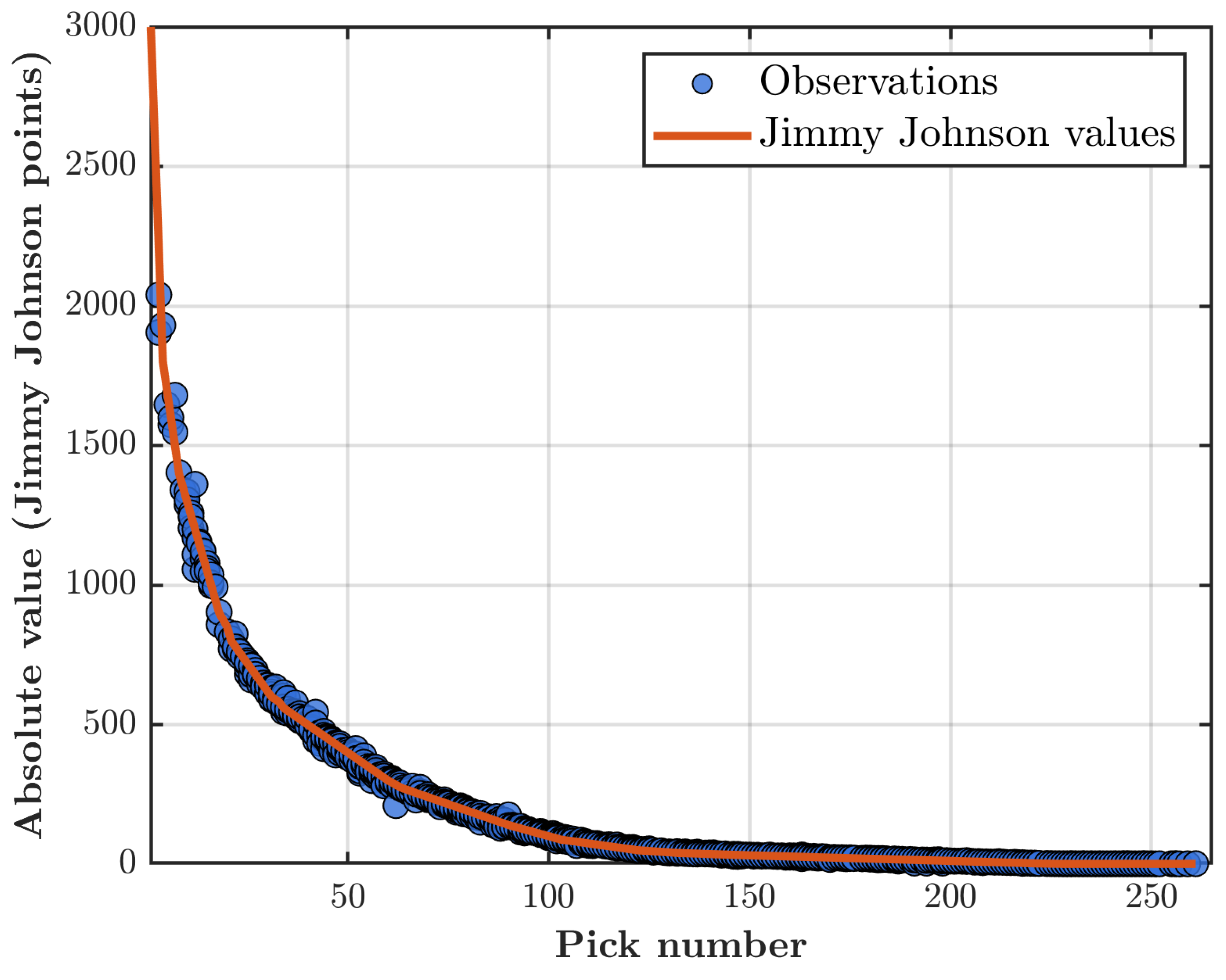
Figure 2.
Transacted values and expected values for the Rich Hill chart (2012-2025).
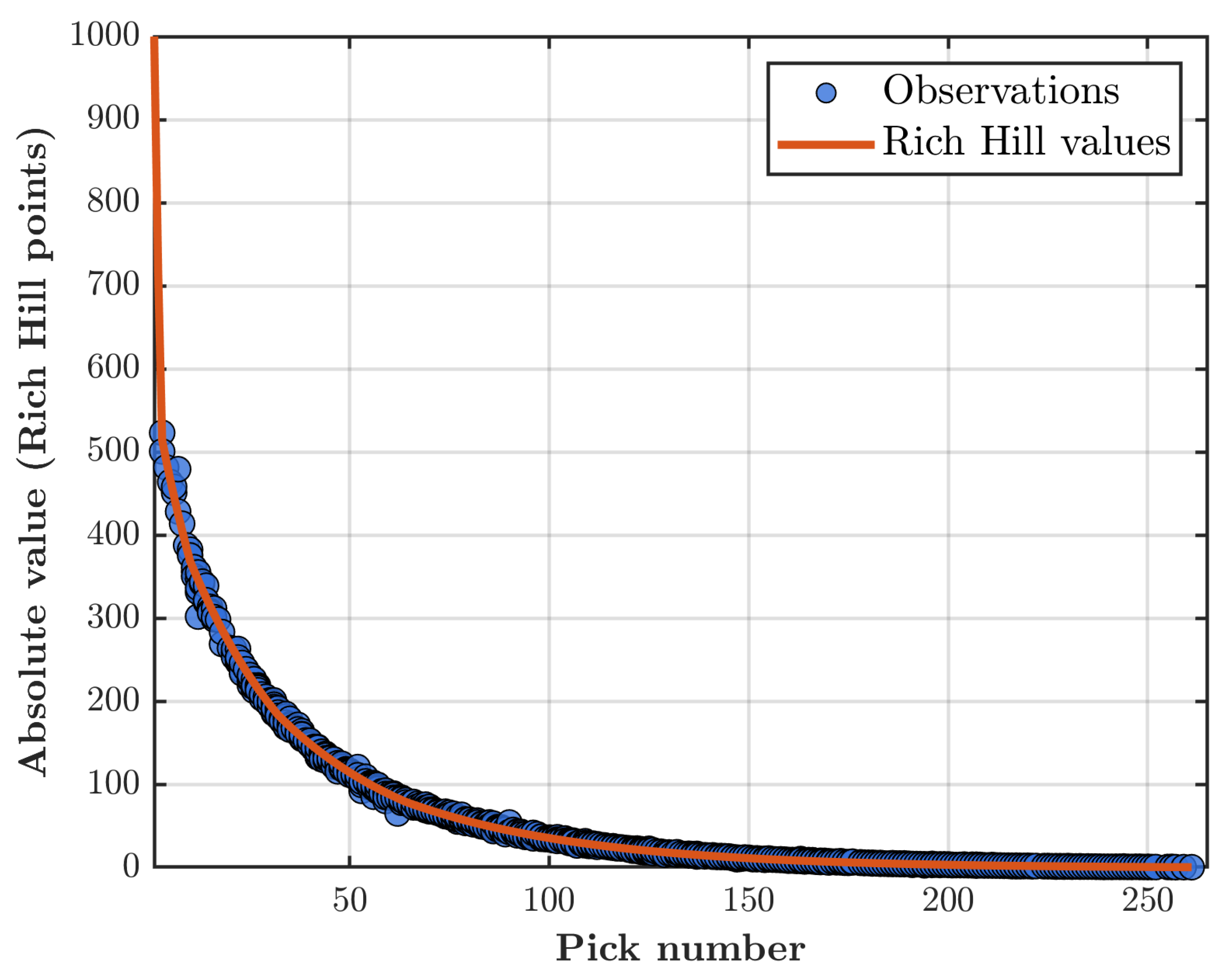
Figure 3.
Comparison of RRMSE values for each pick in the Jimmy Johnson and Rich Hill charts.
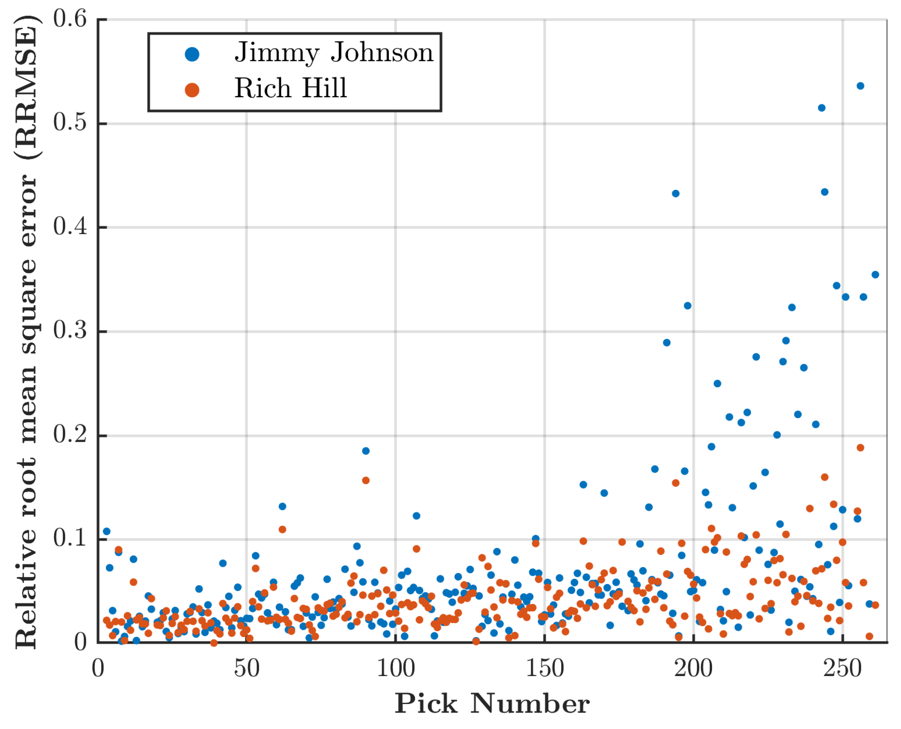
Figure 4.
Heatmap for the custom correlation kernel with variable length scale.
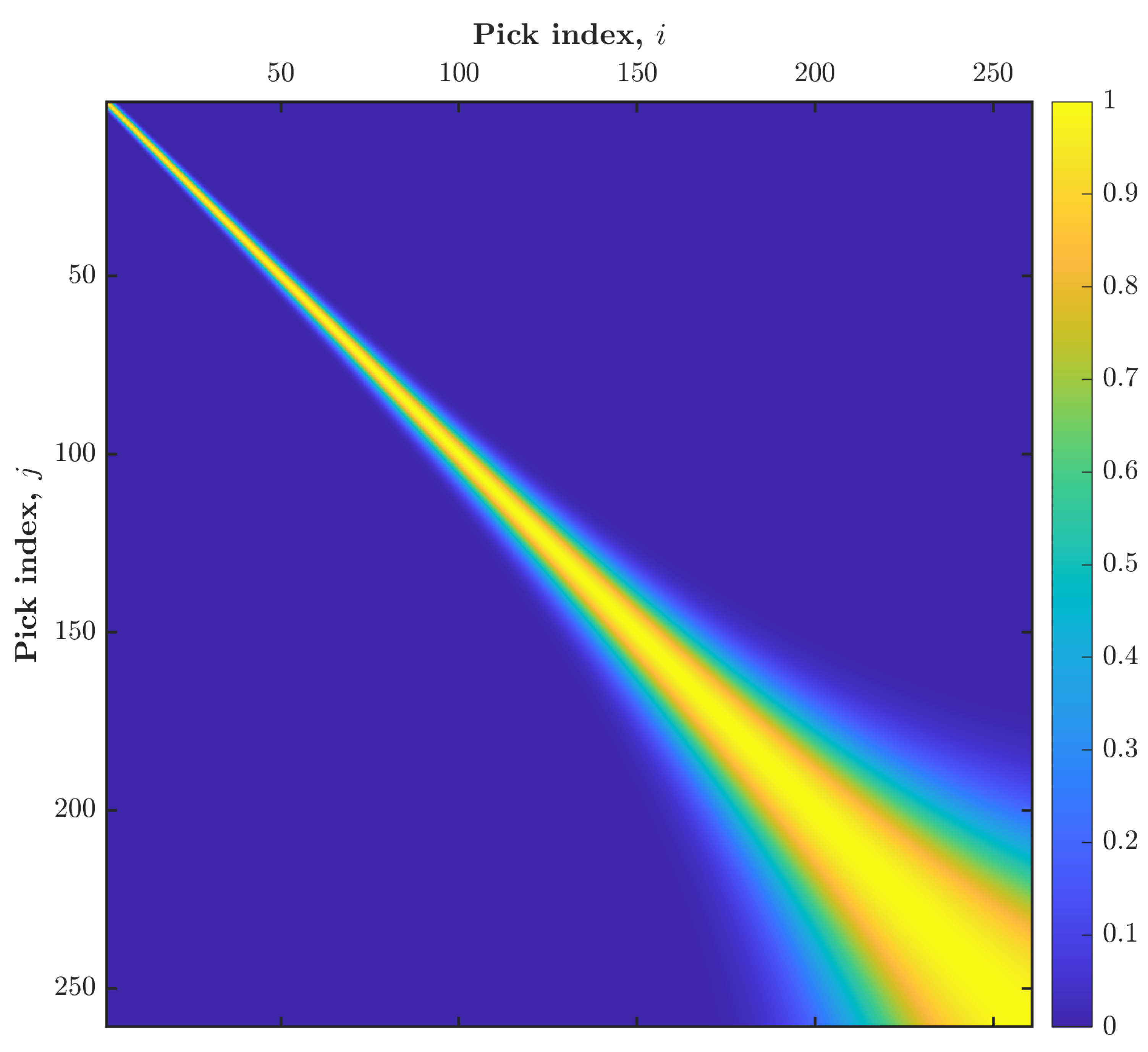
Figure 5.
Comparison between preliminary standard error estimates and the smoothed posterior standard deviation estimates obtained through kernel regression.
Figure 5.
Comparison between preliminary standard error estimates and the smoothed posterior standard deviation estimates obtained through kernel regression.
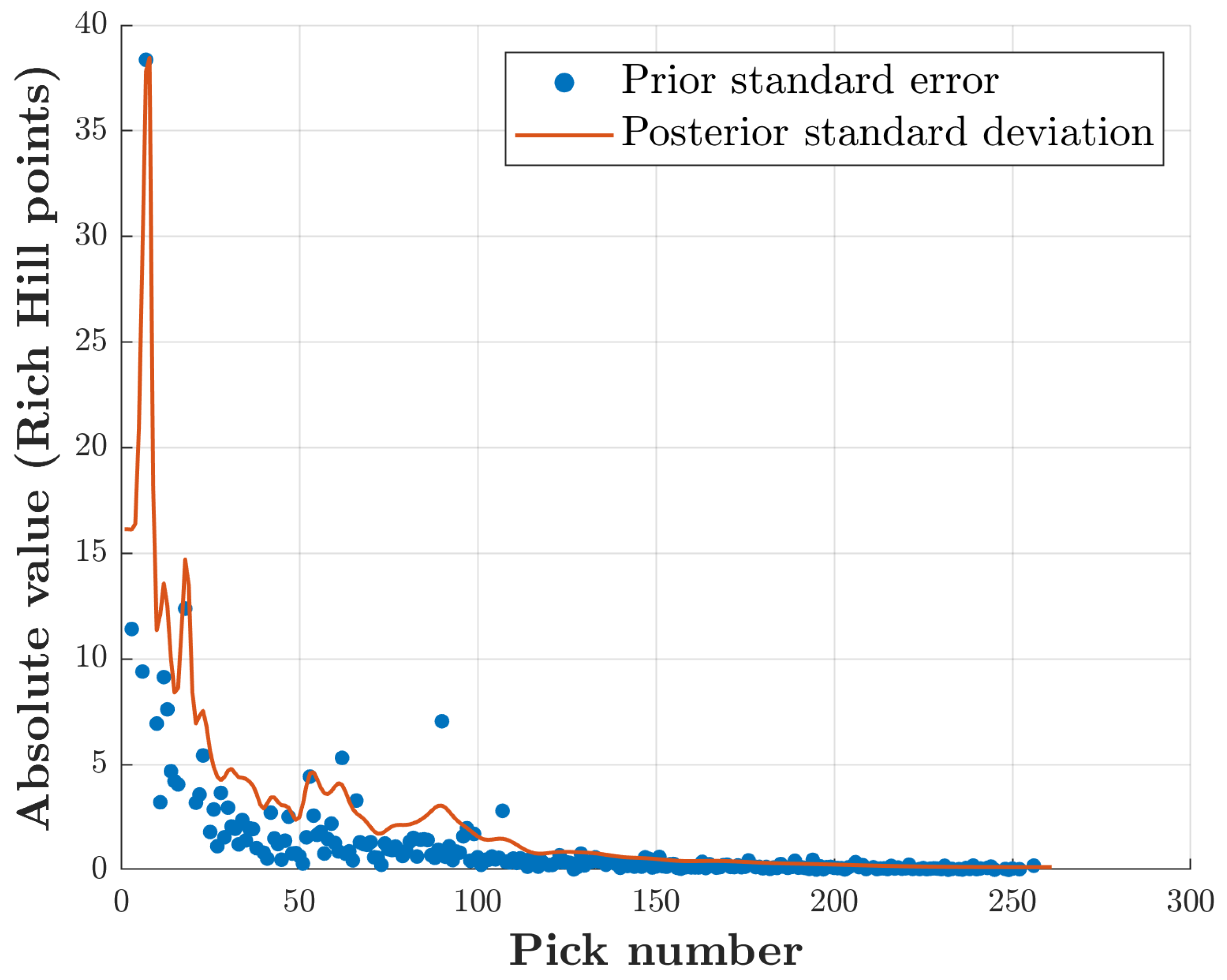
Figure 6.
Confidence intervals (95%) for the transacted values of first round picks.
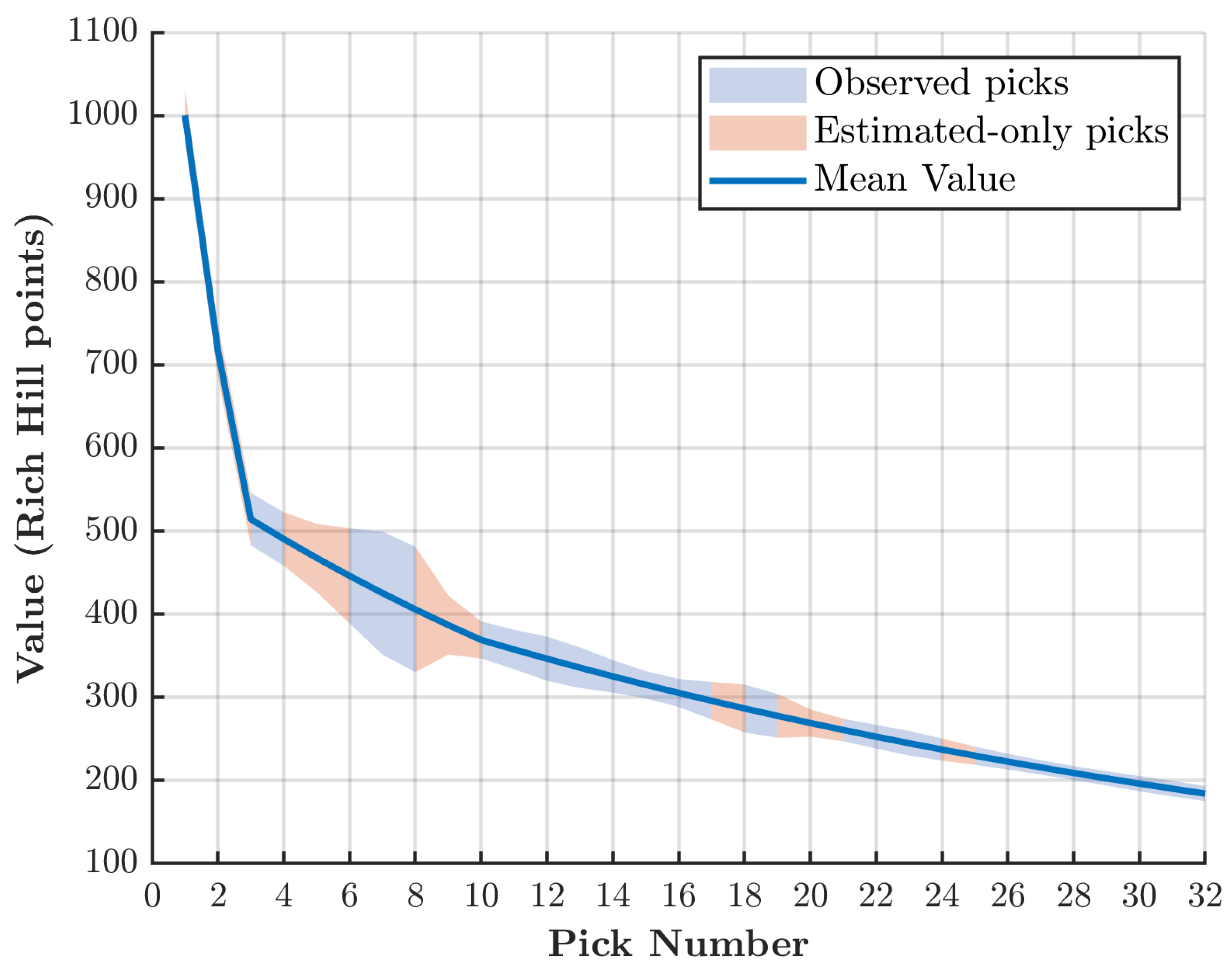
Figure 7.
Confidence intervals (95%) for the transacted values of second round picks.
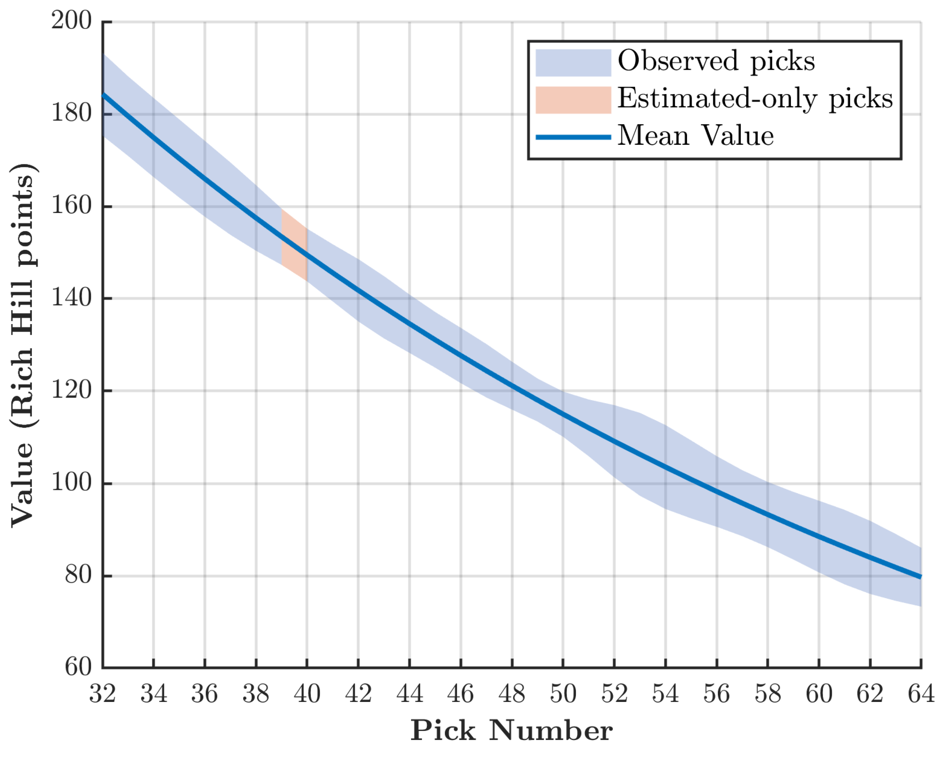
Figure 8.
Comparison of posterior standard deviation estimates obtained using datasets ending in 2024 and 2025. Each point corresponds to the two estimated standard deviations for each pick.
Figure 8.
Comparison of posterior standard deviation estimates obtained using datasets ending in 2024 and 2025. Each point corresponds to the two estimated standard deviations for each pick.
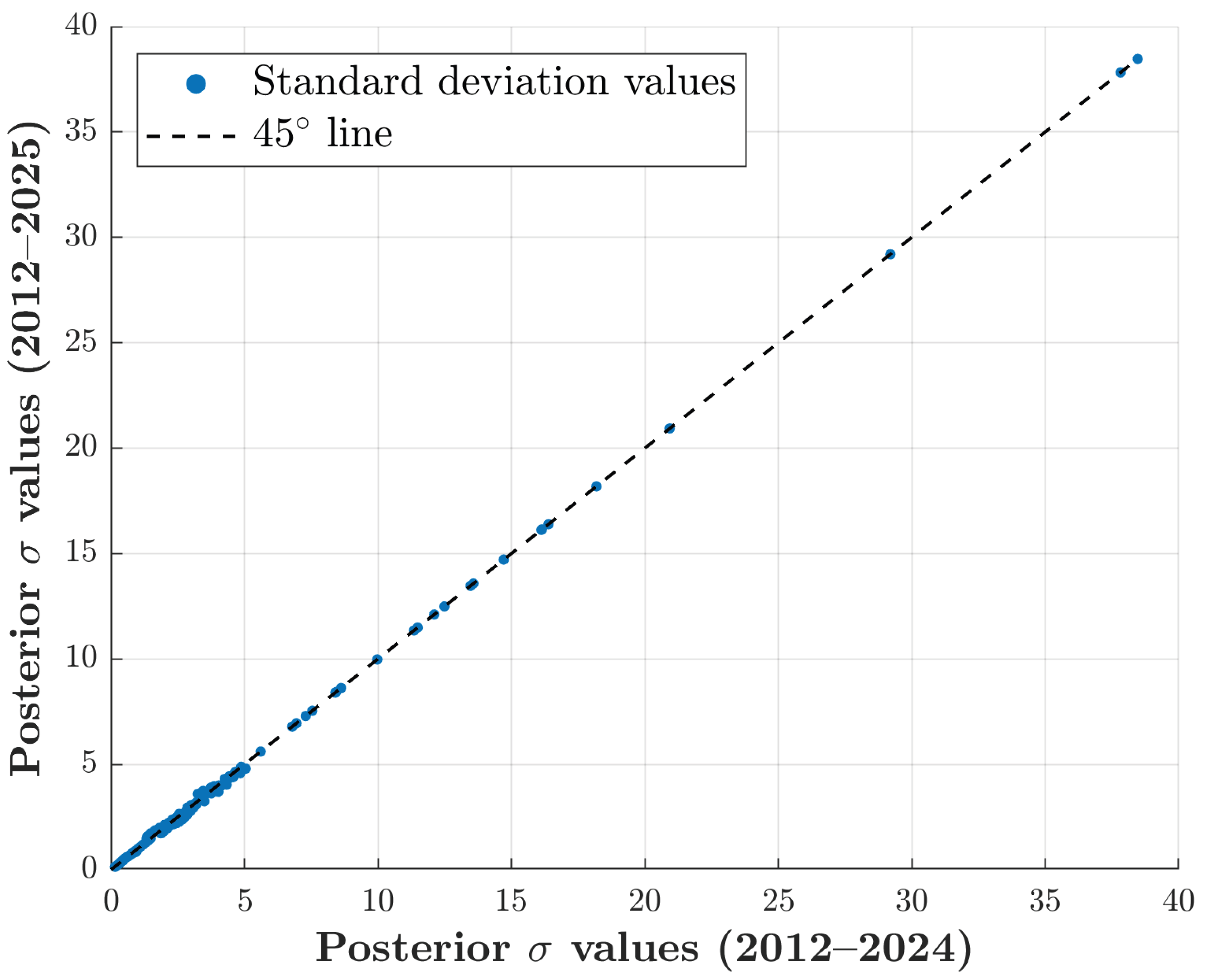
Table 1.
Titans-Seahawks trade (2025 NFL Draft). Values in parentheses correspond to the Jimmy Johnson chart; values in red are from the Rich Hill chart.
Table 1.
Titans-Seahawks trade (2025 NFL Draft). Values in parentheses correspond to the Jimmy Johnson chart; values in red are from the Rich Hill chart.
| Seahawks receive | Titans receive |
|---|---|
| Pick 35 (550 points) (170) | Pick 52 (380 points) (109) |
| Pick 82 (180 points) (54) |
Table 3.
Solution for pick uncertainty (), calculated from the proportionality assumption, for the trade shown in Table 1.
Table 3.
Solution for pick uncertainty (), calculated from the proportionality assumption, for the trade shown in Table 1.
| Pick number (n) | Mean value () | Uncertainty () | Uncertainty (% of ) | Transacted value |
|---|---|---|---|---|
| 35 | 550 | +4.95 | 0.9% | 554.95 |
| 52 | 380 | -3.42 | 0.9% | 376.58 |
| 82 | 180 | -1.63 | 0.9% | 181.63 |
Table 4.
Performance comparison of machine learning methods used to estimate standard deviations of draft pick values.
Table 4.
Performance comparison of machine learning methods used to estimate standard deviations of draft pick values.
| Metric | Kernel Regression | MLE | Random Forest | Gradient Boosting |
|---|---|---|---|---|
| Log-likelihood | -1451.1 | -1451.3 | -1404.9 | -1406.5 |
| RMSEz | 0.9287 | 1.1084 | 1.0804 | 1.0482 |
| Coverage95 | 0.9464 | 0.9840 | 0.9183 | 0.9219 |
Table 5.
Percentiles for the transacted value of each pick in the 2025 Titans-Seahawks trade.
| Seahawks receive | Titans receive |
|---|---|
| Pick 35 (18.31%) | Pick 52 (73.45%) |
| Pick 82 (71.04%) |
Table 6.
Percentiles for the transacted value of each pick in the 2025 Titans–Seahawks trade.
| Seahawks receive | Titans receive |
|---|---|
| Pick 35 (18.31%) | Pick 52 (73.45%) |
| Pick 82 (71.04%) | |
| Grade: 54.6• | Grade: 78.9• |
Disclaimer/Publisher’s Note: The statements, opinions and data contained in all publications are solely those of the individual author(s) and contributor(s) and not of MDPI and/or the editor(s). MDPI and/or the editor(s) disclaim responsibility for any injury to people or property resulting from any ideas, methods, instructions or products referred to in the content. |
© 2026 by the authors. Licensee MDPI, Basel, Switzerland. This article is an open access article distributed under the terms and conditions of the Creative Commons Attribution (CC BY) license (http://creativecommons.org/licenses/by/4.0/).
Copyright: This open access article is published under a Creative Commons CC BY 4.0 license, which permit the free download, distribution, and reuse, provided that the author and preprint are cited in any reuse.