

Submitted:
13 September 2026
Posted:
15 September 2026
You are already at the latest version
Abstract
In this paper, we consider the properties of the following objects: plafal and geo-space (a general overview). As an application of the created theory, the proof of the equality of complexity classes P and NP will be given. The geo-plafal is a kernel (computational template) of the proof; Khomchenko’ scientific school (the constructive theory of serendipity approximations), Stepanets’ scientific school and the Bogolyubov principle of the decay of correlations for an infinite three-dimensional systems is a shell of the proof.
Keywords:
plafal
; plafale
; the theory of plafales
; P vs NP problem
MSC: Primary: 00-02; 00A05; 68Q15; Secondary: 00A71; 08-00; 18A05; 18A10; 37-00; 54-00; 65D99; 65Y20; 68Q25
1. Introduction
The first edition of [1] is published in March 2011. The publication’s goal is the creation of a new theory in mathematics, where the central object is a plafal1. The second edition of [2] is published in February 2013. After the report at the 42nd Polish Conference on Mathematics Applications [3], it is necessary to create applications based on the theory of plafales. Here we will provide the R·D process.
Finite element method. There are created mathematical models of serendipity finite elements: a new approach to construction basis and field functions. A quadruple role of the basis functions of serendipity finite elements is shown [4,5].
IT (finite element method as an algorithmic support). Due to solving the non-standard Dirichlet boundary value problem [4], using the components of the theory of plafales (to obtain the surface of the temperature field in three-dimensional space), there is developed a software for testing non-stationary temperature fields [6].
Cryptography. In September 2014 there is created a symmetric-key algorithm “ECLECTIC-DT-1” [7]. Algorithm’s characteristics: block length is 128 bits, key length is 256 bits, 14 rounds. Let us show the algorithm’s indicators. Upper bounds of practical security: (against differential cryptanalysis [8]), (against linear cryptanalysis [9]). Upper bounds of provable security (for the first four rounds): and . In December 2018 there is created a symmetric-key algorithm “STEEL” [10]. Algorithm’s characteristics: block length is 128 bits, key length is 256 bits, 14 rounds. Algorithm’s indicators: and .
Note. Editions [1] and [2] are the bases of the theory of plafales. The paper presents the “linear passage”: all objects are introduced to prove P = NP as soon as possible. The theory has to be taken into consideration starting from this paper.
2. Concept of the Plafal
We will use a framework “Standard By Default” [11]. A mathematical entity is described as -standard according to the following rules: a set, monoid, topological space, poset, family, graph, diagram, cardinal, ordinal etc. is standard when it is small; a category, groupoid, multicategory, locally ordered category etc. is standard when it is light; for , an n-category is standard when it is n-moderate. A mathematical entity is described as -standard according to the following rules: an ∞-groupoid is standard when it is small; an -category is standard when it is light; for , an -category is standard when it is n-moderate. A function, relation, subset, functor, natural transformation etc. is always standard.
Definition 1.
A plafal is a tuple and is denoted by or , where is a simple graph2, , is a collection of arbitrary -standard, is a collection of correspondences such that we have -standard, , here is a collection of arbitrary -standard that correspond to the vertices; we have -standard, , here is a collection of arbitrary -standard that correspond to the edges. Generally, is called a vertex of the plafal and is denoted by ; is called an edge of the plafal and is denoted by . By we denote a collection of vertices, by we denote a collection of edges. Between and , which are connected by , there is not necessarily a logical relation. If and , then we say that is a trivial plafal and write ∗PF. So, .
For example, the representation of on a vector space is a type of [12].
Remark 1. and . We can operate with and that contain the same entities. Agreement. We claim that , , , . Let us introduce the following notation. is a collection of plafales. is a collection of simple graphs as supports of .
Claim 2.1.
are categories.
Proof.
Let us show for . , , , . □
Let us provide a definition of the plafal within the framework of category theory.
Definition 2.
A plafal is a tuple , where is a 1-dimensional abstract simplicial complex (considering as a category), here is a discrete category of arbitrary -standard, is functor between and such that the above correspondences (see definition 2.1) are performed and morphisms of simplices of and identity morphisms of enteties of are realized.
Definition 3.
Labeled plafal is a type of the plafal, where all or some of vertices and/or edges are enumerated. We have , here and ; , here and ; are substitutions3. By we denote a labeled plafal, k is a quantity of enumerated vertices; l is a quantity of enumerated edges. In the case of , the plafal does not contain enumerated vertices. In the case of , the plafal does not contain enumerated edges. In the case of , we claim that . By τ we denote a vertex with assigned number (), by ς we denote an edge with assigned number ().
Notice that a graph labeling is a type of such that . We consider a labeled trivial plafal as a graph labeling. τ and ς do not necessarily coincide with a number of a graph labeling. Evidently, we can use the following configurations: and .
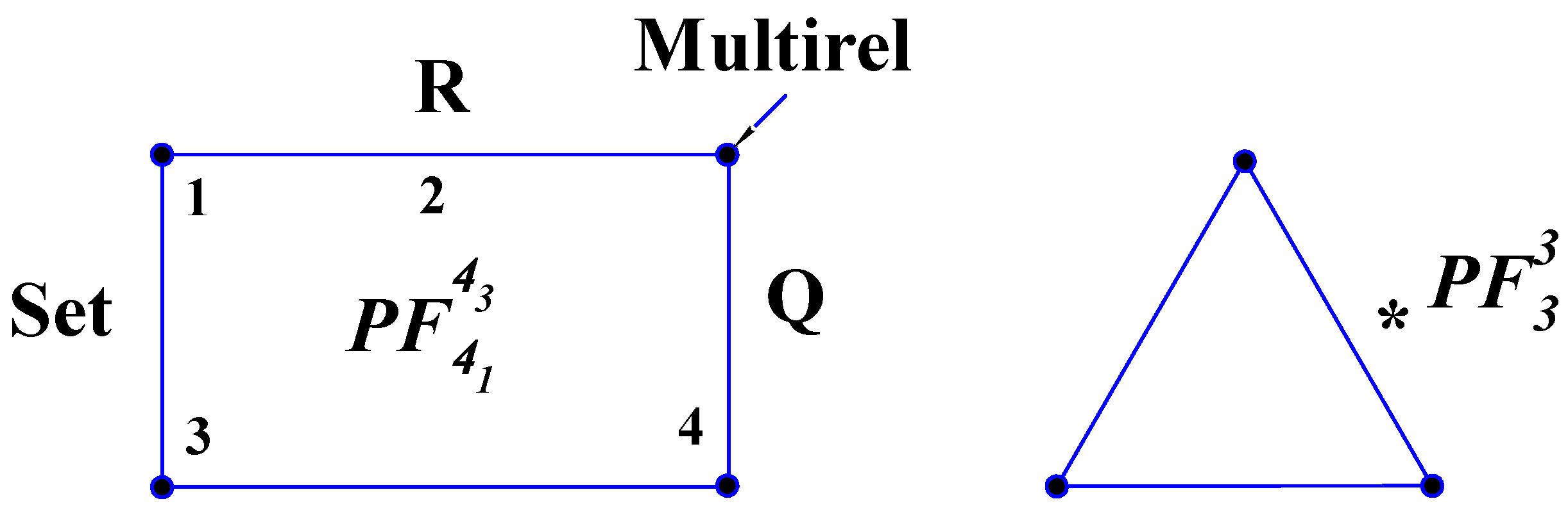
The illustrations of plafales and graphs are given for the reader’s perception.
Figure 1.
. Vertices: (for three vertices), the category of small sets and small multirelations. Edges: the category of sets, the set of real numbers, the set of rational numbers, . Three vertices are enumerated, one edge is enumerated. ∗ is a trivial plafal.
Figure 1.
. Vertices: (for three vertices), the category of small sets and small multirelations. Edges: the category of sets, the set of real numbers, the set of rational numbers, . Three vertices are enumerated, one edge is enumerated. ∗ is a trivial plafal.
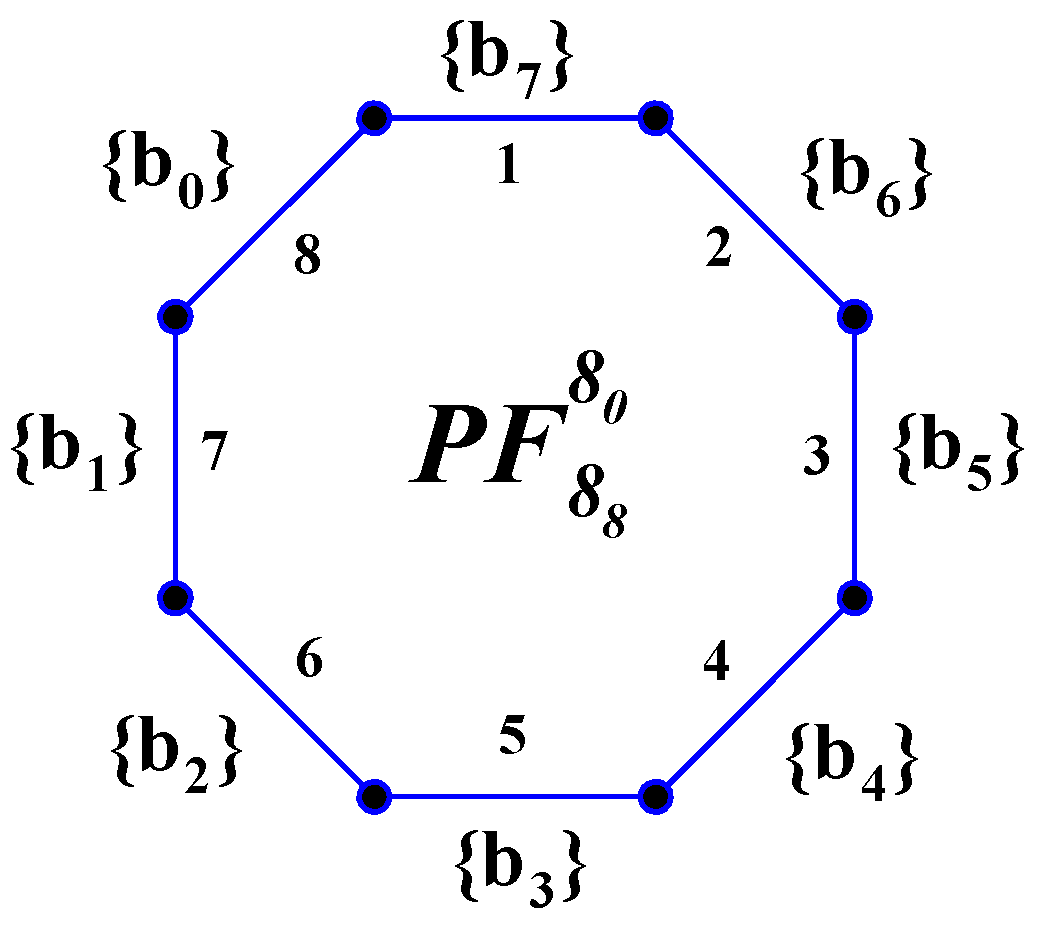
Let us give an example in cryptography [7,10]. For a byte we have the following configurations: ς and .
Figure 2.
. Eight edges are enumerated. The plafal does not contain enumerated vertices.
Definition of an ∗-plafal can be formulated by analogy with the plafal, taking into account we have -standard and we have -standard.
Remark 2.∗-plafales and their properties will be the object of another paper.
3. The Category of Plafales and Operations
Definition 4.
A plafal morphism is a tuple of maps’s collections such that
-
(1) , f is a graph morphism (an abstract simplicial map);(2) : and .Note that (2) is performed in accordance with (1).
The example is given in Figure 3.
Claim 3.1.
Plafales and plafal morphisms form the category Plafales, together with the componentwise compositions and identities . The proof is left to the reader.
Definition 5.
is called an empty plafal and is denoted by , here is the empty graph4 (the initial object in the categories of simple graphs (SimpGph)).
Claim 3.2.
In Plafales, there’re no initial and terminal objects.
Proof.
Initial. Omitted. Terminal. In SimpGph, there’s no terminal object. □
Definition 6.
A product of two plafales is defined by the graph product and the following condition holds:
-
(i) and .Notice that (i) is realized in accordance with ∏.
Definition 7.
A coproduct of two plafales is defined by the graph coproduct and the following condition holds:
-
(i) in the general case, is a coproduct of categories.Let us remark that (i) is performed in accordance with ∐.
Claim 3.3.
In Plafales, the (co)-product of any two plafales does not always exist.
Proof.
It is sufficient to consider and as collections of objects of the category of fields. □
Corollary 1.
Plafales is not a (quasi)-topos. The proof is streightforward.
3.1. Basic Operations
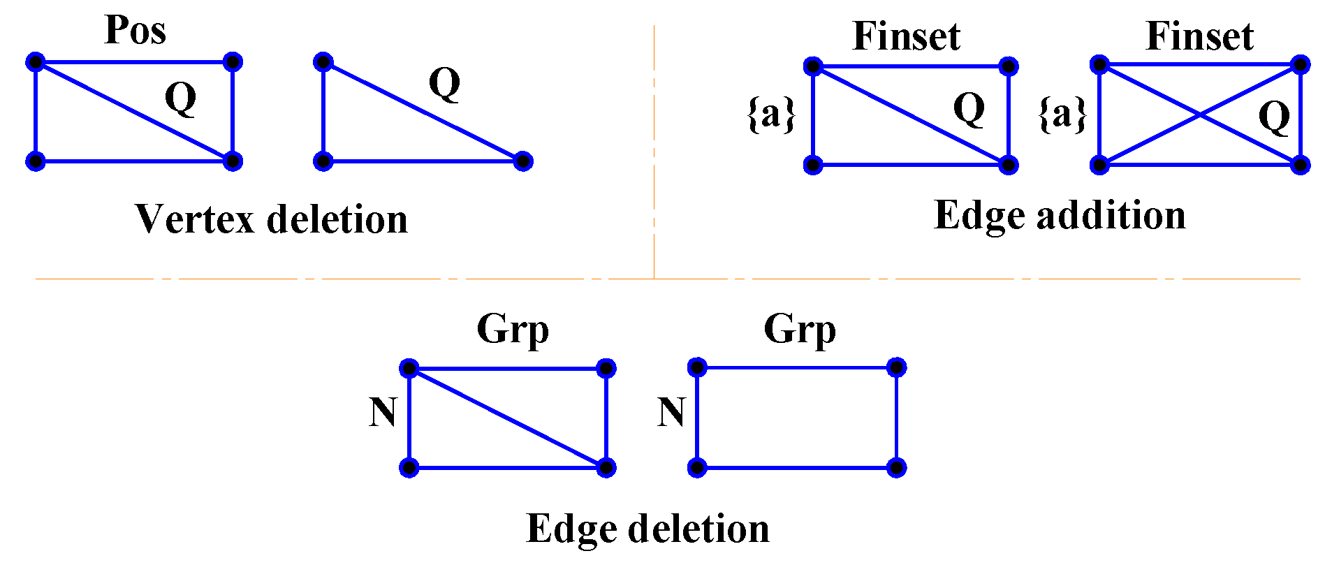
Elementary operations
1. Vertex deletion . 2. Edge deletion . 3. Edge addition .
Figure 4.
Elementary operations.
Advanced operations
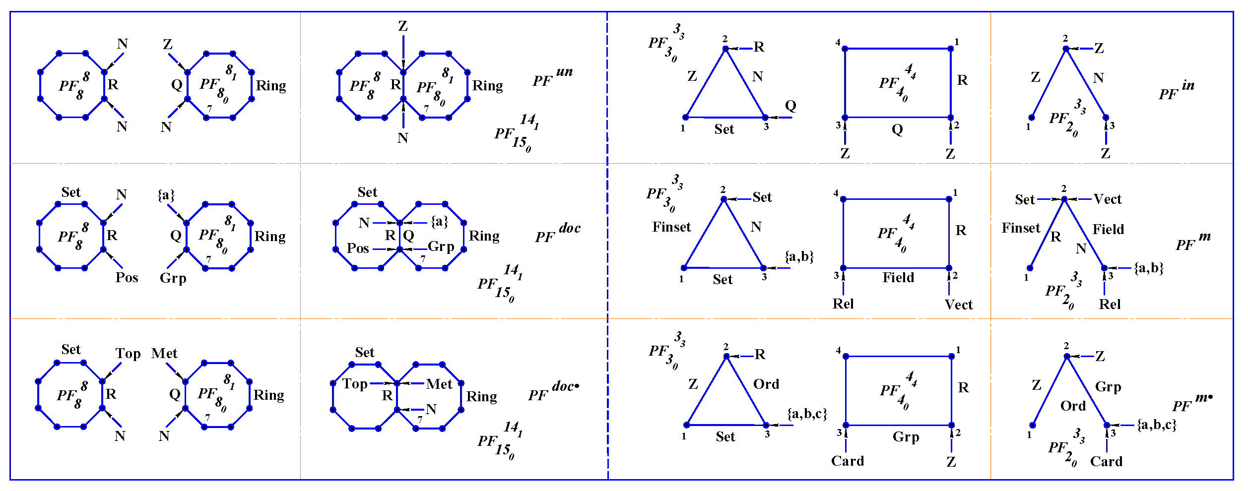
Let us introduce the following notation. is a plafal with assigned number. In the general case, and are the components of and respectively. Let us remark that and are not the entities with specified numbers.
In definitions 3.9 – 3.14, we will use . In definitions 3.9 – 3.11, conditions (i) are performed in accordance with the union of graphs . In definitions 3.12 – 3.14, conditions (i) are realized in accordance with the intersection of graphs .
Definition 8.
A union of plafales is defined by and the following condition holds:
- (i) and .
Definition 9.
A docking of plafales is defined by and the following condition holds:
- (i) and .
Definition 10.
A docking• of plafales is defined by and the following condition holds:
Definition 11.
An intersection of plafales is defined by and the following condition holds:
- (i) and .
Definition 12.
A merger of plafales is defined by and the following condition holds:
- (i) and .
Definition 13.
A merger• of plafales is defined by and the following condition holds:
- (i) Condition (i) of definition 3.12 is performed for common vertices and for common edges; condition (i) of definition 3.13 is realized for common vertices and for common edges.
Agreement7. In definitions 3.10, 3.13, in the case of the chain of operations: , , and taking into account permutations for , we get , where For the same reason, this is performed for .
On the other hand, definitions 3.9 – 3.14 can be formulated in the following form: in general, .
Figure 5.
Advanced operations.
In the case of labeled plafales, and are not labeled plafales, but they can be transformed into the specified types.
Definition 14.
A product• of two plafales is defined by the graph product and the following condition holds:
-
(i) , -standard.(i) is realized in accordance with ∏. The mentioned can be different.
We stress that is a particular case of .
Definition 15.
A decomposition of plafales is a collection of maps such that and the following conditions hold:
-
(i) for k-vertices, which were located at the common vertice, of k-decomposited graphs we have: corresponds to one of the above vertices (k-variations) and there is a collection of arbitrary -standard that correspond to remaining -vertices. By the same argument, this is performed for l-edges;(ii) and remain unchanged;
where is an operation of the decomposition of graphs; here is a collection of and is a collection of for respectively.
Remark 3. The other types of operations will be discussed in a further paper.
4. Geo-Space
Definition 16.
A geo-space is a tuple and is denoted by , where U is a universe of -standard such that .
The objects of the following type , which will be represented in this section, are implemented in . means that U is located outside of . Let us provide a visual perception by analogy in CS. is a directory and U is a collection of external files.
4.1. Geo-Plafal
Let us give a definition of a geometric representation of in .
Definition 17.
is a geo-plafal and is denoted by , is the geometric realization of G in such that in accordance with .
Let us give a comment to definition 4.2. We use the metric or coherent topologies.
On the other hand, can be formulated by analogy with definition 2.1.
Definition 18.
is a geo-plafal and is denoted by or , where is a 1-dimensional simplicial (topological) complex8, , , is a collection of arbitrary -standard, is a collection of correspondences such that we have -standard, , here is a collection of arbitrary -standard that correspond to the vertices; we have -standard, , here s a collection of arbitrary -standard that correspond to the edges. Generally, is called a vertex of the geo-plafal and is denoted by ; is called an edge of the geo-plafal and is denoted by . By we denote a collection of vertices, by we denote a collection of edges. Between and , which are connected by , there is not necessarily a logical relation. If and , then we say that is a trivial geo-plafal and write ∗. So, .
Remark 4. and . We can operate with and that contain the same entities. Claim 2.2, definition 2.3 and definition 2.4 are performed for . Agreement. We claim that , , . By we denote a collection of geo-plafales. By we denote a collection of as supports of geo-plafales.
Definition 19.
A geo-plafal morphism is a tuple of maps’s collections such that
-
(1) , ϑ is a morphism between polyhedra;(2) : and .Note that (2) is realized in accordance with (1).
Claim 4.1.
Geo-plafales and geo-plafal morphisms form the category Geo-Plafales, together with the componentwise compositions and identities . The proof is left to the reader.
Definition 20.
A product of two geo-plafales is defined by the product of polyhedra and the following condition holds:
-
(i) , .Notice that (i) is realized in accordance with ∏.
Definition 21.
A coproduct of two geo-plafales is defined by the disjoint union of polyhedra and the following condition holds:
-
(i) in the general case, is a coproduct of categories.Let us remark that (i) is performed in accordance with ∐.
Claim 4.2.
It is easily proved that such that and is a collection of identity functors, here SCpx is the category of abstract simplicial complexes, Top is the category of topological spaces. Note that advanced operations are performed for geo-plafales. The reader will have no difficulty in showing that , where is a 1-dimensional cellular complex.In Geo-plafales, there’re no initial and terminal objects. The (co)-product of any two geo-plafales does not always exist. Geo-plafales is not a (quasi)-topos. The proof is similar to the proofs in the section 3.
4.2. Point
Definition 22.
is a limit point and is denoted by , where is a limit point in , here is a correspondence such that . If (a singleton in ), then we say that is a trivial point and write ∗.
Agreement. We claim that . By we denote a collection of limit points in . By we denote a collection of limit points in as supports of .
Definition 23.
A morphism is a tuple of maps’s collections such that
-
(1) ;(2) .Note that (2) is performed in accordance with (1).
Claim 4.3.
and morphisms form the category PFpl.
Proof. 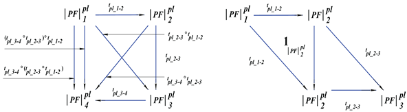
. We get the following commutative diagrams:
□
Remark 5. The concept of with isolated points and the concept of a flickering point, as a superposition of limit and isolated points, will be discussed elsewhere.
4.3. Manifold
Definition 24.
is a manifold and is denoted by , where M is a topological manifold in , here is a correspondence such that . If (an object of 9), then we say that is a trivial manifold and write ∗.
Agreement. We note that . By we denote a collection of manifolds in . By we denote a collection of manifolds in as supports of .
Remark 6. The concept of (open) cover of M (including the relationship with (pre)-sheaf) and a collection of arbitrary , which corresponds to , will be the object of another paper.
Definition 25.
A morphism is a tuple of maps’s collections such that
-
(1) , ϱ is a morphism between topological manifolds;(2) .Notice that (2) is realized in accordance with (1).
Claim 4.4.
and morphisms form the category PFM. Omitted.
Definitions 4.6 and 4.7 (in terms of the product manifold and the disjoint union of topological manifolds) and results of claim 4.8 are performed for .
4.4. Dynamical System
Let us summarize and use the results of [13,14].
Definition 26.
is a dynamical system and is denoted by d, where is a locally compact space satisfies the second axiom of countability and undergoes homeomorphic transformations, here G is a topological group; Ω is a collection of identity functors and results of advanced operations.
Definition 27.
A homomorphism d is a tuple of maps’s collections such that
-
(1) , Φ is a homomorphism between dynamical systems: , μ is a continuous mapping and , is a homomorphic mapping;(2) Δ is a collection of maps between and .Let us remark that (2) is realized in accordance with (1).
The category of dynamical systems is not considered in this paper.
Perspective
Plafal (∗-plafal) complex and plafal (∗-plafal) cell complex are generalizations of the plafal (∗-plafal), and this will be the object of another paper. We will give a short description. For any abstract simplicial complex (n-dimensional cell complex) let there be a correspondence between each face (k-skeleton) and -standard ( respectively).
5. p = np
The proof of the equality of complexity classes P and NP will be given in a constructive way using the apparatus of the constructive theory of serendipity approximations (CTSA)10 [4,15–24]. The total volume of CTSA is about 1000 papers (they can be traced evolutionarily by the indicated references). In the general case, by S we denote an instance of an NP-complete problem. Using the deterministic Turing machine (DTM), C is a type of S with answer “Yes” after the checking, otherwise is . We will operate with a plane in . By we denote this topological subspace. Note that theorem 5.1 is a theoretical model of P = NP; the implementation model of theorem 5.1 on the DTM will be described.
Theorem 5.1.
Based on the theory of plafales, there exists an algorithm that allows to identify all instances of the Boolean satisfiability problem in polynomial time.
Proof. 1st stage. Computational template (CT).
Let us consider the following labeled geo-plafal: , where SFE is a serendipity finite element (square ) on N vertices (nodes)11. Vertices are evenly spaced on the boundary of SFE () by the rule
So, i, is a linear combination such that , , where t is time; .
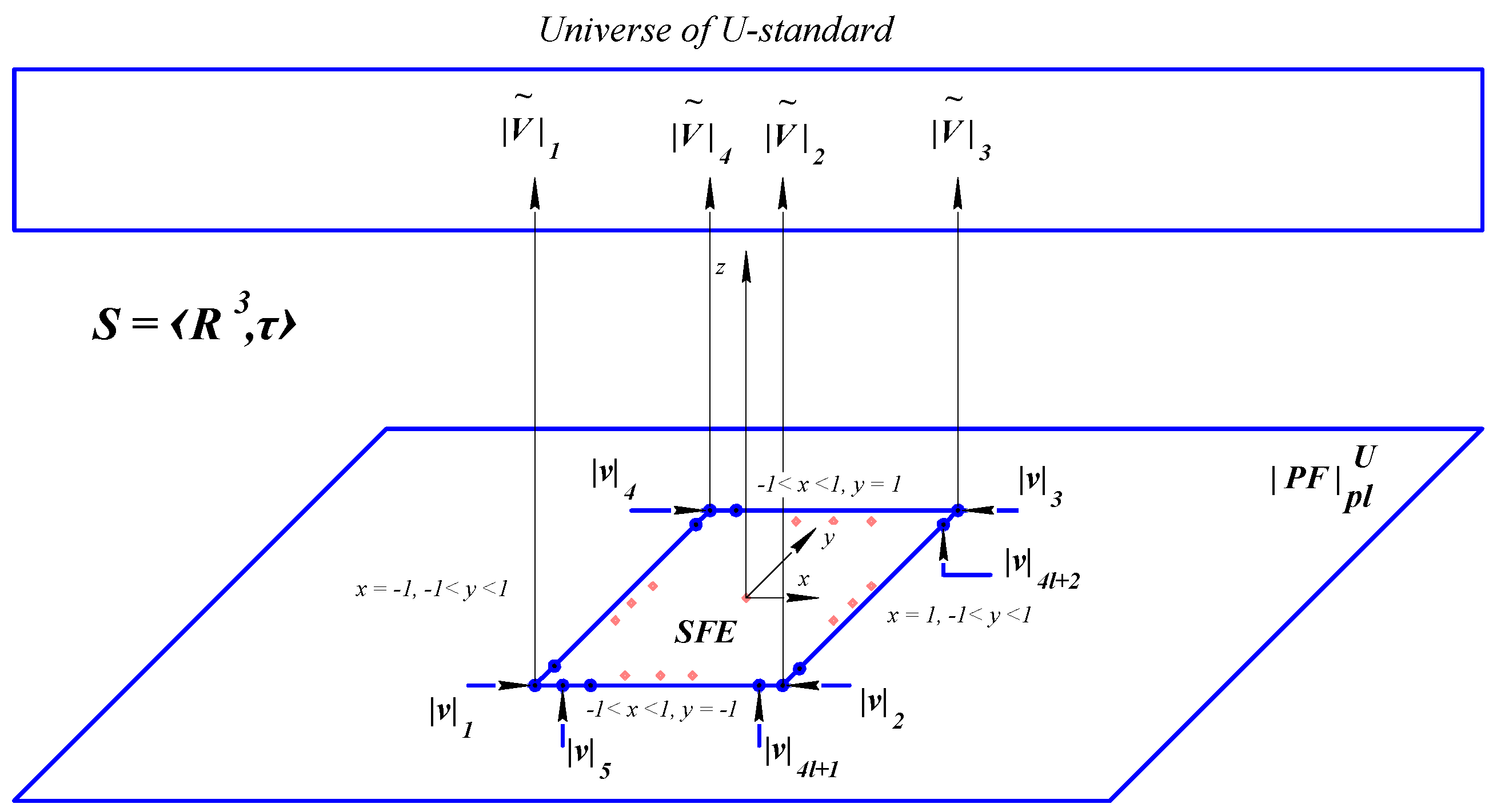
2nd stage. Relationship between and basis function (BF)12 . Let us consider the word over a given alphabet. Then to each corresponds a unique “weight” ; however , here G is the area of D, where N is a quantity of instances of the Boolean satisfiability problem. Hence to each corresponds a unique collection of the basis functions (UCBF) in the CTSA. A relationship between the word and UCBF is structurally shown13.
3rd stage. The analysis of the field function (FF)14. Let us configure the CT. To be precise, (or ). So, we get i.
We will operate with the non-standard Dirichlet boundary value problem [4]. such that Let us comment. For C we get , otherwise is (see Figure 7).
- Taking into account the field function and , let us provide the claim, which is a generalization of the results of Ph. D. thesis [19].
Claim 5.2.
In general, for SFE on N vertices the condition of invariant of the field function (stability of the FF w.r.t. the BF) is the following system
Proof.
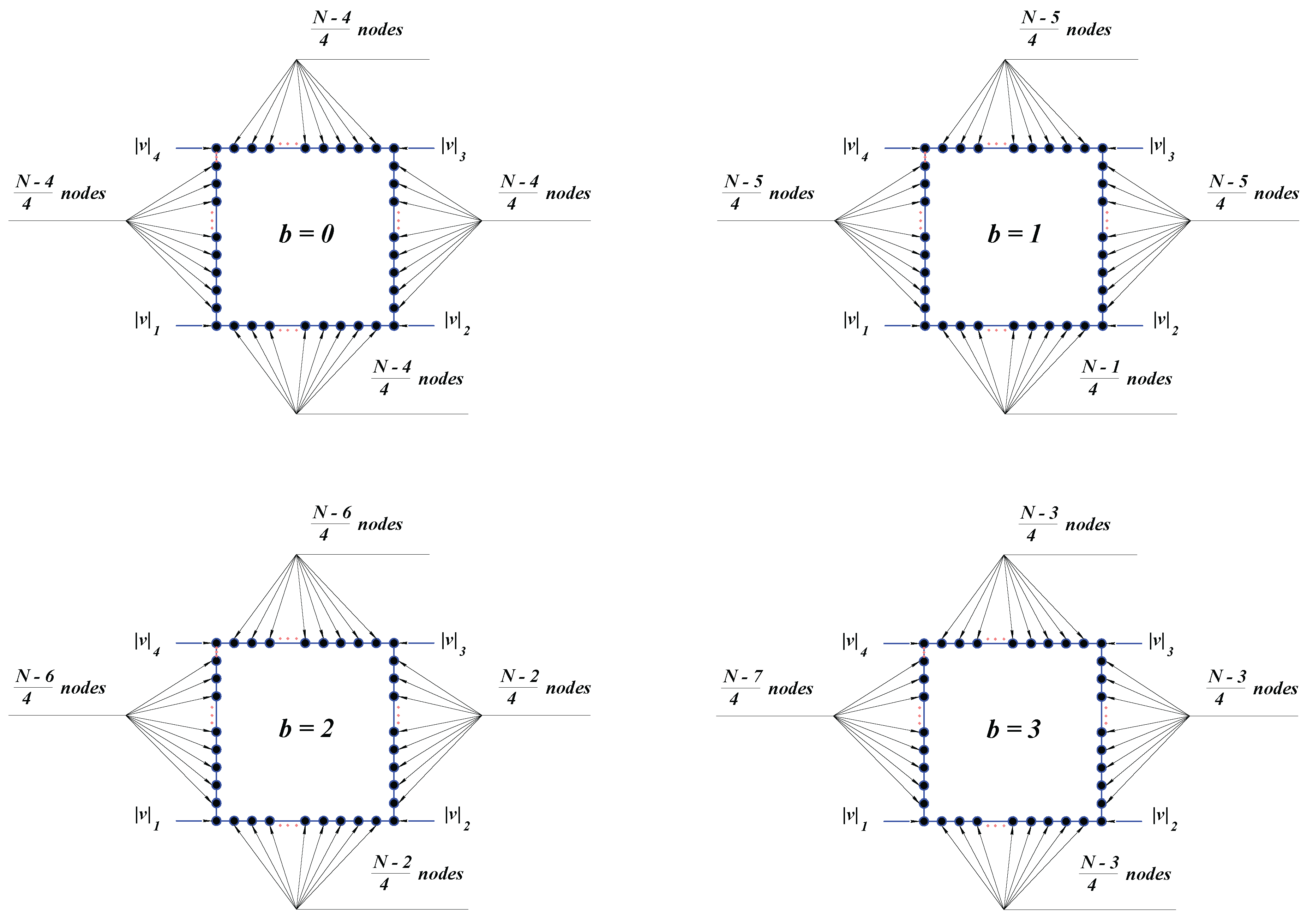
For SFE on 8 nodes the above condition is [4,19]. Let us consider the BF of SFE on N nodes in the following representation: such that Let us show the rule of arrangement of the number of nodes. (see Figure 8). In the case of , b nodes are spaced on b sides of SFE.
is a collection of the basis functions of SFE on 8 nodes [4,17,22]. Therefore, , , , , , , . Let us show one of the collections of the basis functions for SFE·8.
Let us introduce the following system.
Using , we have . Let us remark that , , , .
Taking into account the above condition for SFE·8 and the properties of the BF: we get
and in accordance with coordinates of in we have . Our goal is that the choice of the basis functions is insignificant. So, the expected value of difference of two field functions with different collections of the basis functions is equal to zero. To do that, let us show for the first equation of . and , then , where is a quantity of nodes on the side of SFE (see ).
Let us show for . , here are coordinates in . Thus we obtain . □
Remark 7. There is an additional condition of symmetry of boundary values in some nodes for SFE·12 with n-parametric interpolation () and SFE·16 [19].
Further, we will use the results of Stepanets’ school15. Let us provide the results of [26]. Let be a set of all sequences of nonnegative numbers such that . Let r be a positive number and is a set of all nonincreasing sequences of positive numbers such that . In the case of , we have the following condition: . Denote by a collection of n different integers and for any and , set
and
(i) Let and . Then such that
is determined by
The exact upper bound is realized by the sequence from :
(ii) Let and . Then is performed the following equality
here is the biggest natural number such that
The exact upper bound is realized by the sequence from :
Note. 1. , here is a polynomial. 2. Since solutions of these extremal problems may be of an independent interest, in the paper [26], the authors propose a new method of finding these solutions, which leads to the required result by essentially shorter and more transparent way.
Let us combine all of the above into the following provisions. It is easily shown that the conditions of [26] can be implemented for the field function . Indeed, and it is clear that in the case of values from (6) of . This means that the results of [26] provide an effective tool for the analysis of the field function16. The above results give an opportunity to make the estimate for (word length).
Ideology of P = NP. Due to checking the first M instances (see 1st stage: configuration of nodes) with total computational complexity of , we can identify instances without checking them17, here M is polynomially bounded. Agreement. Without loss of generality it can be assumed that a functional type of is not principled; all required are defined at time . Note that this configuration is an example of the soft mathematical modeling [25].
Let us implement the results of claim 5.2. We can assume without loss of generality that , where is a stabilization function.
Claim 5.3.
The value of the field function at the barycentre18 equals , here , see (i).
Proof.
It is easily shown that , where . Taking into account , by induction, we obtain the statement. □
Corollary 2.
We get , and equals , here , see (ii). The proof is omitted.
Remark 8. Claim 5.3 links two scientific schools: CTSA and Stepanets’ school.
Using claim 5.3, corollary 5.4 and the results of the Bogolyubov principle of the decay of correlations for an infinite three-dimensional systems [27], [28] for the FF (see Figure 7), we have the following system for determination of here .
Let us comment. (4) is the initial-value problem of the BBGKY hierarchy19. Taking into account , for operators (which is defined by the Poisson bracket of free particles with boundary conditions on ) and (in the case of ) we get
Each particle is characterized by the phase coordinates
for impulses : Also for (4) we take into account s-particles correlation functions [27], so
The chaos condition for s-particles correlation functions is as follows [27]:
Note that (5.4) can be obtained on the basis of the solutions of Liouville’s equations.
For a metrizable space the following condition holds: existence of the space of sequences of integrable translation-invariant functions [27]. is a phase space: each z-axis at the node is a particle of unit mass and diameter such that . For (5) we have: taking into account the subscript from (5.1) – (5.4), we operate with (see ★) and define , the number of r is polynomially bounded. For (6) we have are indistinguishable and we take into account . This implies that, .
Let us consider the total computational complexity. 1. Checking the first M instances with total computational complexity of (see ideology of P = NP). 2. The analysis of : 2a. checking with total computational complexity of . 2b. determination of with total computational complexity of . Notice that we use the apparatus of for determination of , instead of item 1, because we use the results of Stepanets’ school (see (i) and (ii)). 2c. Consider the segment as , here each of contains l values such that ; where are polynomials. Determination of each is realized due to permutation with previously defined (we take evenly spaced representatives from each including endpoints) with total computational complexity of . Thus we have leveled the surplus of instances of the Boolean satisfiability problem, so P = NP. □
5.1. The Implementation Model of Theorem 5.1 on the DTM
Using the DTM with polynomial memory, we cannot print on tape all instances of the Boolean satisfiability problem in polynomial time, but we can numerate them on tape in polynomial time. We will operate with polynomially bounded collection of computable values (including () representatives from each (see 2c)) such that the relevant collection of computable “weights” is given (see 2nd stage), is a numerated instance from , is a numerated instance from P.
Using theorem 5.1, we cannot make a permutation between two numerated instances, which are not the representatives from each , because a priori we take into account their unique “weights” (see 2nd stage). Since we operate with polynomial memory, we use the above collection of computable values for the field function.
5.2. General Comments
Section 2.
Certainly, we consider a plafal as a deep extension of decorated graph.
Section 5.
1. To avoid conflicts, we operate only with universe of the Boolean satisfiability problem, where the implementation model of theorem 5.1 is an emulator. That is why, theorem 5.1 is not a universal algorithm (specifically, for the TSP). We work with computable values in , but not with universe of directly.
2. Constructive theory of serendipity approximations. Let us show the procedure of constructing of the basis function in accordance with (customised BF).
(1) ⇒ (2), where is a weighted coefficient, and are given loads of well-known basis functions and respectively. This is a comment for the 2nd st.
Let us provide an alternative apparatus for (see 2nd, 3rd stages). We can use a substitute basis function . Let us show the key properties. and , where is the Kronecker delta, here i is a number of function and k is a number of node.
Historical background. Dual role of the basis functions of serendipity finite elements is proved by O. Zienkiewicz (1968). His group constructed a biquadratic basis (SFE·8), but Zienkiewicz’s paradox is formed: in some nodes exist negative loads (unnatural spectrum). In 1982 Khomchenko constructed a 13-parametric bicubic basis (SFE·12) with positive loads [20,21], thus Zienkiewicz’s paradox was solved. Methods of constructing alternative (physically correct) bases are presented in [16].
3. The paper is performed in the spirit of “The science absolute of space: independent of the truth or falsity of Euclid’s axiom XI (which can never be decided a priori)” by J. Bolyai: rigorism that is tailored to the reader’s background.
4. The article was 16 years in the making. AI was not used.
Perspective. Using the quantum Turing machine (QTM), theorem 5.1 is performed for (here is a vector in Hilbert space (see 1st stage)).
5.3. Appendix
Let us give a strengthening of the results [26] in the case of .
Let be a set of all sequences of real numbers such that
and . Let also N be a fixed positive integer and be a set of all nonincreasing sequences of nonnegative numbers such that .
Denote by a collection of n different integers and for any and , set
and
Lemma 1.
Let . Then for any
In this case, the exact upper bound on the right-hand side of the relation (5.6) is realized by the sequence such that
Proof.
Let be a set of all sequences such that . Then
Indeed, let . We construct a sequence such that .
Step 1. If , then represent the number in the form , where . Consider the sequence such that
Since , we have , , and . If , then we set .
Step 2. If , we represent the number in the form , where . Consider the sequence such that
Similarly, we have , , and . If , then we set .
Step N. Continuing this procedure, at Nth step we finally construct the sequence such that , and . Setting we see that it satisfies all the necessary relations.
By virtue of (5.5), for any sequence we have
To finish the proof it is sufficient to make sure that the sequence of the form (5.7) belongs to the set and
□
Acknowledgments
Mathematics: A. N. Khomchenko (D. Sc., Petro Mohyla Black Sea National University), V. V. Lyubashenko (D. Sc., Institute of Mathematics of the NAS of Ukraine), A. A. Novikov (Ph. D., Novikov Labs), O. V. Rybak (Ph. D., Kyiv Polytechnic Institute), A. L. Shydlich (D. Sc., Institute of Mathematics of the NAS of Ukraine). Cryptography: L. V. Kovalchuk (D. Sc., Kyiv Polytechnic Institute). Thank you for your critical comments and consultations. Personal participation: O. Borisenko, D. Chibisov, A. Druz, A. Evseev, A. Kulyeshov, M. Malaev, J. Milej, V. Obod, A. Sinchuk, O. Topchyi, W. Topolski, R. Valiullin, M. Vialkov, Yazeed Abdulrahman. I am really grateful for your help.
List of Key Terms
– plafal; ∗ – trivial plafal; – plafal with assigned number
– vertex of the plafal; – edge of the plafal; – collection of -standard
– collection of ; – collection of plafales
τ – vertex with assigned number; ς – edge with assigned number
– labeled plafal; – empty plafal
– product of plafales; – coproduct of plafales
– union of plafales; – docking of plafales
– intersection of plafales; – merger of plafales
– geo-space; – geo-plafal; ∗ – trivial geo-plafal
– product of geo-plafales; – coproduct of geo-plafales
– limit point in ; ∗ – trivial point in
– manifold in ; ∗ – trivial manifold in
d – dynamical system; – plane in
| 1 | The singular form is a plafal or a plafale. Pl: plafales. |
| 2 |
G is a 1-dimensional abstract simplicial complex that does not contain an isolated vertex. Generally, v is a vertex of , e is an edge of . V is a collection of vertices, E is a collection of edges. For G we have the following: a vertex is a singleton; an edge is an unordered pair. |
| 3 |
is a bijection iff ; is an injection iff . is a bijection iff ; is an injection iff . |
| 4 |
(see definition 2.1). |
| 5 |
r is a quantity of common vertices. |
| 6 |
t is a quantity of common edges. |
| 7 | We use this agreement only as a recommendation. |
| 8 |
is a polyhedron that does not contain an isolated vertex. Generally, is a vertex of , is an edge of . is a collection of vertices, is a collection of edges. |
| 9 |
is the category of topological manifolds. |
| 10 | Constructive theory of serendipity approximations is a branch of Bernstein’s school of constructive function theory and A. N. Khomchenko is the founder of this scientific school [20,21]. Note. S. N. Bernstein presented in a constructive way (1912) the Weierstrass theorem (1885). |
| 11 | Serendipity finite element is a finite element that does not contain interior nodes. |
| 12 | Let us show the key properties of the basis function. and , where is the Kronecker delta, here i is a number of function and k is a number of node. |
| 13 | In fact, this relationship acts as a “lock” (hard model [25]) such that ↔ UCBF. This enables us to determine based on , here is a value of the FF at a given node . |
| 14 | The field function (interpolant) makes an interpolation on the boundary of SFE and an approximation inside of SFE. |
| 15 | In the series of works, O. I. Stepanets’ and his successors study approximation properties of the spaces introduced by Stepanets’. Problems of finding exact values of n-term approximations of q-ellipsoids in the spaces considered are reduced to some extremal problems for series with terms that are determined as a product of elements of two nonnegative sequences one of which is fixed and another varies on certain set. |
| 16 | We are able to evaluate all “fluctuations” of the field function (according to all possible shifts). |
| 17 | We are able to level the specified surplus of instances, N (see 2nd stage). We are interested in the case when M instances is a collection of (see preamble). Our goal is to determine a position number of C in instances or to identify that all instances are . |
| 18 | Taking into account the results of Khomchenko’s school and Mbius’s problem (1827), we are able to manage the integral characteristics of the basis function at the barycentre. |
| 19 | The Bogolyubov (Bogoliubov) - Born - Green - Kirkwood - Yvon hierarchy. |
References
- Topchyi, D. The theory of plafales, 1st edition; Best Global Publishing: UK, 2011; 634 p. [Google Scholar]
- Topchyi, D. The theory of plafales, 2nd edition; Best Global Publishing: UK, 2013; 695 p. [Google Scholar]
- Topchyi, D. The theory of plafales: applications of new cryptographic algorithms and platforms in military complex, IT, banking system, financial market. In 42nd Polish Conference on Mathematics Applications; Polish Academy of Sciences: Warsaw, 2013; p. 58. [Google Scholar]
- Topchyi, D. Models of the serendipity family, methods and software for testing non-stationary physical fields. Ph. D. thesis, Mykolaiv, 2017. 152 p. [Google Scholar]
- Topchyi, D. The theory of plafales: quadruple role of the basis functions of serendipity finite elements. Review of results. Scientific Works of Vinnytsia National Technical University, 2016, no. 2, pp. 72 – 78.
- Topchyi, D. The software “Testing of non-stationary temperature fields with dynamic thermoelements”. Electronic scientific journal “Branch aspects of technical sciences”, Publishing house INGN, 2015, iss. 4 (46), pp. 27 – 37.
- Topchyi, D. The theory of plafales: cryptographic complex “ECLECTIC-DT-1”. UK, Chipmunkapublishing, 2015, 65 p.
- Lai, X.; Massey, J. L.; Murphy, S. Markov ciphers and differential cryptanalysis. Advances in Cryptology, EUROCRYPT’91, Proceedings. Springer Verlag, 1991, pp. 17 – 38.
- Matsui, M. Linear cryptanalysis methods for DES cipher. Advances in Cryptology, EUROCRYPT’93, Proceedings. Springer Verlag, 1994, pp. 386 – 397.
- Topchyi, D. The theory of plafales: symmetric-key algorithm “STEEL”. 72 p. [CrossRef]
- Levy, P. B. Formulating categorical concepts with classes. arXiv:1801.08528. [CrossRef]
- Gelfand, I. M.; Ponomarev, V. A. Gabriel’s theorem is also true for representations of equipped graphs by relations. Funct. Anal. Appl. 1981, 15, 71–72. [Google Scholar] [CrossRef]
- Barbashin, E. A. On homomorphisms of dynamical systems. Mat. Sb. (N. S.) 1950, 27, 455–470. [Google Scholar]
- Barbashin, E. A. On homomorphisms of dynamical systems 2. Mat. Sb. (N. S.) 1951, 29, 501–518. [Google Scholar]
- Astionenko, I. A.; Litvinenko, Ye. I.; Khomchenko, A. N. Cognitive-graphic analysis of hierarchical bases of finite elements; Oldi-plus, 2019; 259 p. [Google Scholar]
- Astionenko, I. A.; Litvinenko, Ye. I.; Khomchenko, A. N. Construction of the multiparameter polynomials by the bicubic element of serendipity family. Scientific reports of Belgorod State University. 2009; 5, pp. 15–31.
- Astionenko, I. A. Models of approximation of functions by multiparameter polynomials of the serendipity family. Ph. D. thesis, Kherson, 2011. 180 p. [Google Scholar]
- Huchek, P. Y. Development of geometric models and computer programs for function restoration problems. Ph. D. thesis, Kherson, 1998. 162 p. [Google Scholar]
- Kamaeva, S. O. Geometric models and methods of the constructive restoration of physical fields. Ph. D. thesis, Kharkiv, 2010. 218 p. [Google Scholar]
- Khomchenko, A. N. FEM: some probabilistic questions. VINITI: 1213, 1982, 9 p.
- Khomchenko, A. N. FEM: stochastic approach. VINITI: 5167, 1982, 7 p.
- Khomchenko, A. N.; Tuluchenko, G. Y. Geometric modeling on discrete elements; Oldi-plus, 2007; 270 p. [Google Scholar]
- Litvinenko Ye, I. Mathematical models and algorithms of computer diagnostics of physical fields. Ph. D. thesis, Kherson, 1999. 172 p. [Google Scholar]
- Tuluchenko, H. Y. Geometric modeling of scalar fields by the method of the averaging of adaptive invariant templates. Dr. thesis, Kherson, 2008. 425 p. [Google Scholar]
- Arnold, V. I. Hard and soft mathematical models. MCCME, 2008, 32 p.
- Stepanets’, O. I.; Shydlich, A. L. On one extremal problem for positive series. Ukr. Math. J. 2005, 57, 1968–1976. [Google Scholar] [CrossRef]
- Gerasimenko, V. I.; Shtyk, V. O. The Bogolyubov principle of the decay of correlations for an infinite three-dimensional systems. Reports of the National Academy of Sciences of Ukraine, 2008, vol. 3, pp. 7 – 13.
- Gerasimenko, V. I.; Gapyak, I. V. Advances in theory of evolution equations of many colliding particles. Modern problems of mathematics and its applications. Proceedings of the Institute of the NAS of Ukraine, 2023, vol. 20, iss. 1, pp. 729 – 804.
Figure 3.
Condition 1. The image of under the strict homomorphism is . Condition 2. U is a functor; g is a homomorphism of groups.
Figure 3.
Condition 1. The image of under the strict homomorphism is . Condition 2. U is a functor; g is a homomorphism of groups.
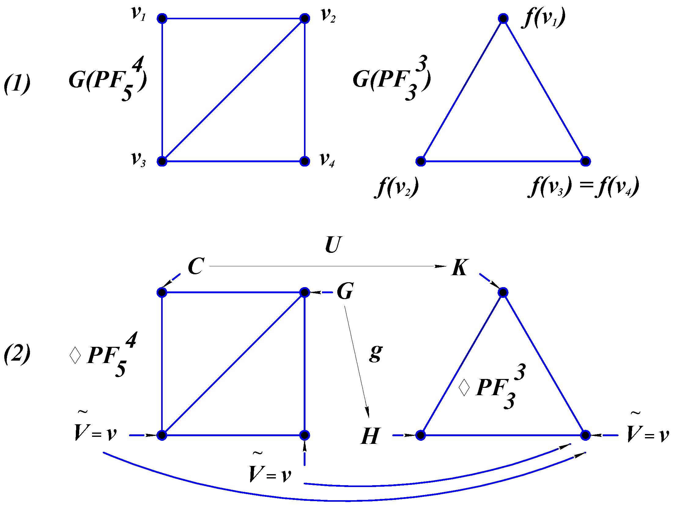
Figure 7.
The field function.
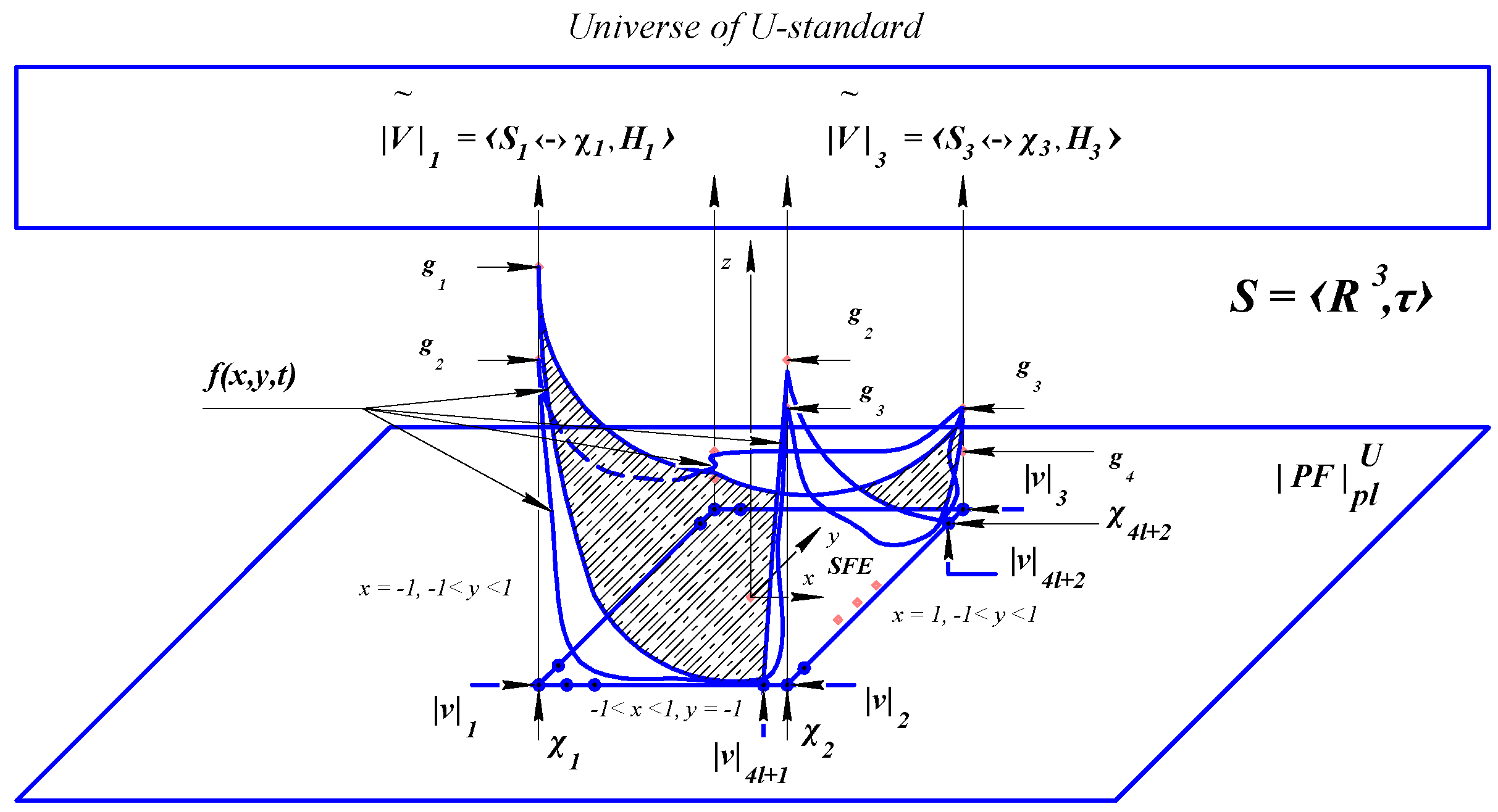
Figure 8.
Configuration of nodes.
Disclaimer/Publisher’s Note: The statements, opinions and data contained in all publications are solely those of the individual author(s) and contributor(s) and not of MDPI and/or the editor(s). MDPI and/or the editor(s) disclaim responsibility for any injury to people or property resulting from any ideas, methods, instructions or products referred to in the content. |
© 2026 by the authors. Licensee MDPI, Basel, Switzerland. This article is an open access article distributed under the terms and conditions of the Creative Commons Attribution (CC BY) license (http://creativecommons.org/licenses/by/4.0/).
Copyright: This open access article is published under a Creative Commons CC BY 4.0 license, which permit the free download, distribution, and reuse, provided that the author and preprint are cited in any reuse.