

Submitted:
26 February 2026
Posted:
03 March 2026
You are already at the latest version
Abstract
In this work, we present a generic classification of a class of n-dimensional piecewise smooth vector fields known as refractive systems. Our purpose is to characterize the local structural stability of refractive fold-folds of elliptic type. To this end, we reduce the study of such piecewise smooth vector fields to the analysis of the first return maps and their structural stability. Normal forms for such systems are also provided.
Keywords:
piecewise smooth vector fields
; structural stability
; singularities
MSC: 34A36; 34D30; 37C10; 37G05
1. Introduction
The theory of dynamical systems is a powerful tool for the study of systems whose state changes over time. Today, this theory is well developed for smooth systems. However, several problems are modeled by systems that exhibit discontinuous behavior, such as systems that involve friction or impact. Examples of such systems arise in control theory [1], biology [2] and various other areas.
In this text, we work with local properties and therefore we use the notion of germs of mappings and vector fields. Let p be a point and let A and B be two neighborhoods of p (in some global topological space). We say that and are germ-equivalent at p if there exists a neighborhood of p such that f and g coincide on C. As the name suggests, germ-equivalence is an equivalence relation. A germ of a function at p is its equivalence class in the germ-equivalence. The germ of f at p is denoted by or, in the extensive notation, . If we require that , we denote . A representative of a germ is a (global) function that belongs to this equivalence class.
Throughout this text, unless stated otherwise, we do not make distinction between functions and germs of functions. Germs of functions and germs of vector fields will be referred simply by functions and vector fields, respectively, if there is no risk for ambiguity.
Let be the function defined by We define the set
which separates the space in the two open regions
Let X and Y be two smooth (class , r large enough) vector fields around the origin. We define a piecewise smooth vector field by
The set is called switching boundary or simply boundary.
Let be an open set with compact closure containing the origin. Denote by , or simply , the set of smooth vector fields in U. Endow with the topology. We consider the space of piecewise smooth vector fields defined in U being with the product topology.
The points where are called tangency points (or Σ-singularities) of X. Here denotes the Lie derivative of relative to X at p.
A point that satisfies and is called a fold point. If , we say that p is a visible fold while if , p is said to be an invisible fold of X. If and , we say that p is a cusp point of X.
In an analogous way, we define fold and cusp points of Y. However, the inequalities of visibility are reversed: for visible folds and for invisible folds.
A point is called a fold-fold point if it is a fold of both vector fields X and Y. A fold-fold point p is called hyperbolic if it is a visible fold of both fields, elliptic if it is an invisible fold of both fields, and parabolic if it is a visible fold of one field and an invisible fold of the other (Figure 1).
Definition 1.
A refractive system is a piecewise smooth vector field satisfying for all .
In a refractive system, there are no sliding or escaping regions, only crossing regions and tangency points. Also, if a point in the boundary is a tangency point of one of the fields, then it must be a tangency point of the other.
A local trajectory of through a point is a curve that satisfies and . A local orbit of a point is the image of a local trajectory of this point. The orientation of an orbit is the orientation induced by the trajectory.
For refractive systems, we define local trajectories as follows.
Definition 2.
Let be a refractive vector field defined in . A local trajectory of Z through a point is a curve satisfying
- (i)
- If (respect. ) then is the usual trajectory of X (respect. Y) through the point p in (respect. ).
- (ii)
- If is a crossing point1 then, in the case , we define for and for , where and are the usual trajectories of the fields X and Y through p. An analogous definition can be done when .
- (iii)
- For tangency points, if it is possible to extend the definitions of the trajectories at points of the boundary near p, then the local trajectory is defined as being this extension. If it is not possible to extend the definition, we define the local trajectory of p as being the constant curve .
Let and be two refractive vector fields defined in the open sets and , respectively, both sets containing the origin. We say that and are Σ-equivalent if there exists a homeomorphism that preserves the boundaries (i.e., ) and carries orbits of to orbits of preserving the orientation of the orbits.
We say that a refractive vector field Z is (globally) structurally stable if there exists a neighborhood of Z such that every refractive system in B is -equivalent to Z.
The definition of local -equivalence is analogous to the definition above, just considering h as a germ of homeomorphism.
A germ of a refractive vector field is said to be structurally stable if it admits a structurally stable representative.
It is worth to say that the definition of structural stability above is relative to the space of refractive vector fields. Some fold-folds are structurally stable in the space of refractive systems (as we will see later) whereas fold-folds are never structurally stable in the context of general vector fields.
For definitions on general theory of piecewise smooth dynamical systems (Filippov systems) we refer the reader to the texts [3,4], for example, and references therein.
The main motivation for the study of refractive systems comes from the work of Ivar Ekeland [5] about Variational Calculus published in 1977. In this work, the author establishes results on existence of solutions for a one-dimensional variational problem and presents a local classification of what are now called refractive systems in the plane. In 1984, Fopke Klok [6] studied the same problem for two-dimensional systems, adding a homogeneity hypothesis to the system.
Another example of an application of refractive systems arises when we consider a discontinuous ODE of order
where and
for and smooth functions.
When we introduce the variables for and , the resulting system is a first-order refractive ODE. This type of system appears, for instance, when we work with forces () including friction in the system. Another example where this type of construction appears is in the modeling of blocks over surfaces in motion. This model is used in the study of earthquakes. See [7,8,9] for more details.
A recent study that uses the construction above was done by Jacquemard, Pereira and Teixeira [10] in the so-called relay systems. These systems can be described by the equation
where are smooth functions and .
This paper is organized as follows. In Section 2, we describe the main results and the methodology used in this paper. In Section 3, we prove that the structural stability of the fields can be reduced to the structural stability of the first return maps. In Section 4, we find the series expansion of the first return maps up to the second-order terms. In Section 5, Section 6, Section 7 and Section 8, we prove the main results of this text.
This work presents the results obtained in Siller’s doctoral thesis [11], where the proofs of the main results and the methodology of this paper are developed.
2. Main Results
Throughout the next sections, denotes the j-th coordinate of x, that is, if then . and denote the sets and respectively.
In this text, we are concerned with local structural stability of n-dimensional refractive fold-fold systems around the origin.
Denote by the space of germs of fold-fold refractive vector fields at . Every hyperbolic refractive fold-fold has the same topological behavior around the origin. It is not difficult to find a local -equivalence between any two hyperbolic refractive fold-folds. The same occurs with the parabolic ones. Therefore, the hyperbolic and parabolic refractive fold-folds are structurally stable on .
On the other hand, the behavior of the elliptic refractive fold-folds is more complicated and their classification is not trivial. The main purpose of this work is to characterize the structural stability of these systems. To this end, it is natural to reduce the study of the systems to the analysis of their first return maps.
Let be the space of germs of elliptic refractive fold-fold systems at . When we take a system we can assume, without loss of generality, that it satisfies:
- (P1)
- Z is a germ of a system around the origin;
- (P2)
- and therefore the boundary is ;
- (P3)
- The set of tangency points of Z is ;
- (P4)
- The field Y is ;
- (P5)
- The last coordinate of the field X is .
Below we briefly discuss these properties.
The first two properties are already considered since the beginning of this text. For the property (P3), the set of tangency points of Z is a codimension-one submanifold of and, by a smooth change of variables, it can be assumed to be . The property (P4) is known as Vishik Normal Form of Y. See [12,13] for more details.
The Property (P5) is non-trivial. Since Z is a refractive system, we have that
However, it may fail to hold for points outside the boundary. As the origin is a fold point of X, the -th coordinate of X satisfies and
Moreover, from (P3), for . So
and therefore . By the Implicit Function Theorem, there exists a smooth function such that
So, the set of points x near the origin where is the codimension-one submanifold
After the change of variables
for the points where , the manifold M becomes
Then the -th coordinate of X can be written as for some smooth and positive function .
Define the positive scalar function by
for and otherwise. Since in the boundary and it is piecewise smooth, the function s is clearly continuous and positive near origin.
Multiplying the field X by s, we have that becomes for all x near the origin and therefore we have Property (P4).
Since X is a fold at the origin, the trajectory of each point (unless the tangency points) hits the boundary at another point (Figure 2). For the tangency points, we define . The function is a map associated to X that satisfies
- is an involution, that is, ;
- is smooth. It can be seen applying the change of coordinates given by Vishik in [13], noticing that in these coordinates the involution becomes the smooth functionand then returning to the original coordinates.
- , where denotes the set of fixed points of .
In an analogous way, we can define the involution associated to Y. From (P4), is the involution
Denote the set of fixed points of . Let
The first return map of Z is the application given by
Remark 1.
For the region , the first return map is defined as . However, such map is conjugate to defined on and therefore they are topologically equivalent. Hence we can restrict the domain of the first return map to the set .
Since , the map can be written
where is a function. In Section 4 we study the series expansion of .
So, each can be associated to a smooth function . The main result is described in terms of such mappings.
Theorem 1.
The field is structurally stable on if, and only if, either
- (a)
- (Regular case), or
- (b)
- (Singular case) and F is hyperbolic at 0.
Here, the hyperbolicity of F is understood in the sense of vector fields, that is, all the eigenvalues of its derivative have nonzero real parts. For this reason, from now on, F is regarded as a vector field on .
The proof of this theorem is divided in the following three lemmas.
Lemma 1
(Regular case). If then Z is structurally stable on .
Lemma 2
(Singular case). If and F hyperbolic at 0, then Z is structurally stable on .
Lemma 3
(Converse). If and F is non-hyperbolic at 0, then Z is not structurally stable on .
The normal forms are expressed in the following result.
Theorem 2.
[Normal Forms] A field is structurally stable if, and only if, it is Σ-equivalent to one of the following normal forms
- (a)
- Regular case: with ;
- (b)
-
Singular case: for somewith hyperbolic and .
Where .
The particular case of Theorems 1 and 2 for dimension 3 was already proved by Buzzi, Medrado and Teixeira in [14]. The authors reduce the study of elliptic refractive fold-folds to the analysis of the associated first return maps. For the regular case, the authors have proved that the first return map is conjugate to its linear part and therefore it is structurally stable. The main tool used in the proof is a result in [15] which states that every planar diffeomorphism with linear part is conjugate to this linear part. However, such result actually does not hold in general. A counterexample is given by the map which has the curve as an invariant set. The orbits of the points on this curve converge (in positive or negative time) to the origin, whereas the orbits of its linear part are parallel to the x-axis.
Here we use the same methodology as in [14]. For the regular case, we prove that the first return map is conjugate to its linear part. We introduce an additional hypothesis that allows us to construct a conjugacy between the first return map and its linear part. For the singular case, we prove that the first return maps are conjugate to their perturbations. The proofs of Lemmas 1 and 2 are given in Section 5 and Section 6, respectively.
3. First Return Maps
In this section, we establish the equivalence between the structural stability of an elliptic refractive system and of its first return map.
For each , denote by its first return map. Since the trajectories depend continuously on the vector fields, the application j is continuous.
Let be the space of germs of involutions on such that . Denote by the space of compositions
As observed in the previous section, we assume that the functions in are restricted to the region .
To prove the main result of this section, we use the lemma below. The proof of this lemma is similar to that given in [14], adapted to arbitrary dimension.
Lemma 4.
Let . The systems and are Σ-equivalent at the origin if and only if and are conjugate.
Proof.
Suppose and are -equivalent and let h be a -equivalence between these fields. The boundary is invariant by h. We claim that h restricted to conjugate and .
Indeed, let . The orbit of leaving p intersects again at the point . As h is an equivalence between and , the orbit of through intersects at . On the other hand, by the definition of , the orbit of through intersects at . It follows that . The same argument applied to and shows that . Therefore
and and are conjugate.
Conversely, assume that some homeomorphism conjugates and . Denote by the flow of , for . For each point near the origin, define and such that
Let be the functions satisfying
that is, is the time that the trajectory of takes to reach again by the field . Define
For , set . This function is clearly continuous.
Now define analogous functions and for the field , that is, satisfying
The function defined by
is continuous and it is easy to show that is the inverse of the function H around the origin. So H is a local homeomorphism over and is a -equivalence between the fields and .
In the same way, we define obtaining a function H defined in a neighborhood of the origin. The function H coincides with when restricted to and with when restricted to . Hence H is continuous and, applying the same argument to , we conclude that H is a local homeomorphism around the origin. Therefore H is the desired -equivalence and it follows that and are -equivalent. □
Let be the involution in given by
By Lemma 4 and Property (P4), for each map in there exists a change of coordinates so that it can be written as for some involution .
The main result of this section follows.
Theorem 3.
Let . If is structurally stable on , then Z is structurally stable on .
Proof.
Suppose that is structurally stable on . Then there exists an open set containing such that all are conjugate to . By the continuity of j, there exists an open containing Z such that . It follows, by Lemma 4, that every is -equivalent to Z and therefore Z is structurally stable on . □
The converse of Theorem 3 also holds, however this assertion is not applied here and we do not prove it. A proof for the two-dimensional case can be found in [14].
4. Series Expansion of First Return Maps
Recall that the first return map associated with an elliptic refractive field is a map of the form , where is an involution with . It follows that can be written as
We can write in the following way
where we decompose the last coordinate in terms that contain exactly one factor and terms that contain at least two factors in the series expansion of . We also require that .
Computing the last coordinate of the expansion of , we have
As is an involution, is the identity function and therefore
So
for all x near the origin. When , we have
By the continuity of the right-hand side expression, this equality also holds when . Replacing , it follows that
As f is continuous and , we conclude that f is identically zero. Therefore the involution has the following format
In the case where all are zero in (2), the map can be written as
where A is an matrix. Rewrite in the following form
The first coordinate of is
But as is an involution, and therefore
and
What interests us is expression (4). Clearly, the same arguments hold for all coordinates and therefore we have
The last coordinate of is given by
and therefore follows
The next sections are devoted to prove Lemmas 1, 2 and 3 and Theorem 2.
5. Lemma 1
In the following sections, we are restricting the diffeomorphisms to the region . From (3), the first return maps can be written as
For satisfying the conditions of Lemma 1, we have
To prove Lemma 1, we use the following auxiliary result.
Lemma 5.
Consider a diffeomorphism φ with the format (6). The linear part of φ is given by
where . If , then φ is locally conjugate to its linear part.
Proof
(Proof of Lemma 1). Let be as in Lemma 1. The linear part of is the transformation with . By Lemma 5, is conjugate to its linear part.
There exists such that every map in with has its linear part having the form with . Again by Lemma 5, is conjugate to its linear part.
Therefore, is conjugate to for all with . It follows that is structurally stable on and, by Theorem 3, Z is structurally stable on . □
The remainder of this section is devoted to the proof of Lemma 5.
Consider a diffeomorphism as in (6). Its linear part is given by (7) and suppose that . The following lemma reduces the form of (7) to a simpler one.
Lemma 6.
The linear transformation is conjugate to
Proof.
Take a change of variables that preserves the -axis and sends the vector to . □
Therefore, from now on, we will suppose that the derivative has the form given in (8).
For each , define the following function
We extend for all in the following way
where is the -th iterate of . For each x, the curve is the union of straight line segments connecting to for . The function is continuous in x and t and smooth when . The curves are right-differentiable in t for all x.
The notation does not create ambiguity with the notation of the iterates , since both definitions coincide when . It is worth noting that, despite the notation, the curves are not flows of vector fields, since we cannot guarantee the relation when a and b are not integers.
Lemma 7.
For each , the transformation is a diffeomorphism around the origin.
Proof.
For , we have
Then
So and the result follows by the Inverse Function Theorem. The result for follows immediately. □
Define the transversal to the map (that is, the vectors are transverse to in a neighborhood of the origin). Let
(Figure 3). The following lemma states that the orbits of points near the origin always cross this transversal.
Lemma 8.
There exists a neighborhood V of the origin such that for all there exists an integer with (see Figure 3).
The proof of the lemma above depends on the following algebraic result.
Lemma 9.
Let and be two sequences of real numbers satisfying
- label=
- for all .
- lbbel=
- for some .
- lcbel=
- for some .
Then .
Proof.
Consider the sequence . This sequence satisfies
Let
We have that .
Notice that the fixed points of are 0 and and that between these two values. We must have for all i. Indeed, otherwise we would have which would imply , contradicting the condition a.
If then . If then and therefore exists such that . So is increasing for i large enough and it is bounded by 1. Therefore the sequence is convergent. It is easy to see that .
So, for small enough, there exists such that for all . Then
for all . Therefore
when as we want to demonstrate. □
Proof
(Proof of Lemma 8). Let V be a bounded neighborhood of the origin such that for all . As the closure of V is compact, there exists some constant such that for all .
Let . Define the sequences and as being the first and the n-th coordinate of the terms of the orbit , that is, and . Define also the sequences and such that , , and (we can assume that V is small enough such that is always positive).
We have
and
Taking V smaller if necessary, we can assume that for all i. We know that and, supposing that for some j, we have
since the function is increasing in the interval . It follows, by induction, that and then for all i with . Notice that the sequences and satisfy the hypothesis of Lemma 9 and therefore . It implies that there exists such that and therefore , as we want to demonstrate. □
By the same arguments as above, we can prove
Lemma 10.
For all there exists an integer such that .
From Lemmas 8 and 10, it follows that the orbit of each point in V crosses (in positive or negative time) the transversal .
Thus, it is possible to define two functions and such that . In other words, for each point , the curve intersects the transversal at the point and at time . These functions are clearly continuous.
Define
where . This function is continuous and well-defined in a neighborhood V of the origin intersected with .
We prove that the function h can be extended continuously to the region (taking V smaller, if necessary), and this extension conjugates the map with its linear part . To do it, we need a sequence of lemmas.
Lemma 11.
The function π is locally Lipschitz at the origin2.
Proof.
Let and write .
Consider a bounded neighborhood V of the origin such that the orbit of every point in crosses the transversal , that and the angle between and is less than for all .
Since the closure of this neighborhood is compact and F is continuously differentiable, there exists a constant such that for all , where denotes the usual norm in the space of matrices. This implies that
Take two points and in and let . Consider the reparametrizations and of the curves and , respectively, such that its derivatives in the first coordinate are equal to 1, that is, and .
Consider the function . For each t, there exists such that the curve is a line segment for all time between t and . This segment connects points of the form and for some integer . Let be the vector in the direction of this segment such that its first coordinate is 1 (that is, is the right derivative of in t). In the same way, we define the vector for the curve . For sufficiently small, we have
However, for each , the vector has the form for some . It follows that
So
If , then is a decreasing function in the interval .
In the other hand, if , we have
Then
for . By the same argument for , we have
Since the neighborhood V is bounded, the function is bounded and therefore there exists such that
Finally, consider the points , and . They form a triangle with .
We have , . Then
This estimation holds for any two initial points and so the proof is reached. □
Lemma 12.
There exists a neighborhood of the origin in which the function π satisfies
for all in this neighborhood.
Proof.
Consider a bounded neighborhood V of the origin such that for all (remember we are assuming by (8)).
As F is continuously differentiable and V has compact closure, there exist constants such that and for all . So we have
for . We can assume, without loss of generality, that .
If is the angle between and , we have that
and this inequality holds for all . Remember that by (6). It means that the angle between and the horizontal hyperplane containing x is less than .
Therefore, the point must satisfy
By intersecting V with the region where , we have the left-hand inequality.
On the other hand, let be the reparametrization of by the first coordinate, that is, the and have the same image and . From (9) we have that
where denotes the right-derivative of . Hence
and therefore
By intersecting the neighborhood with the region where , we obtain the right-hand inequality. The case is analogous. □
Lemma 13.
The function is locally Lipschitz at the origin
Proof.
Let V be a bounded neighborhood of the origin such that for all . We also assume that V satisfies the conditions of Lemma 12. There exist constants such that and in V.
Let and in V. We assume, without loss of generality, that .
Define the curves
the function difference and
The curves and v are right-differentiable and we denote by its right-derivatives, respectively. The notation denotes the right-derivative of with respect to time t.
We want to maximize the value of for each t. From Lemma 12, for , we have
Therefore, for ,
The curve hits the transversal in time for . Then and . Since , then
We also have
From
it follows that
Since and , it follows that the function is Lipschitz in V. □
From the Lemmas 11, 12 and 13, it follows:
Corollary 1.
The function is locally Lipschitz at the origin.
We now combine the previous Lemmas to show that h is well behaved.
Lemma 14.
The function h is locally Lipschitz at the origin.
Proof.
This follows straightforwardly from Corollary 1. □
Finally, we prove the main lemma of this section.
Proof
(Proof of Lemma 5). From Lemma 14, we can extend the function h continuously to the region . This extension is clearly a local homeomorphism around the origin. We claim that h conjugates the diffeomorphisms and .
First, notice that (Lemma 6). If , then and therefore . If , we have
and
which finishes the proof. □
The proof of Lemma 5 concludes the proof of Lemma 1.
6. Lemma 2
The approach for Lemma 2 is somehow similar to that done for Lemma 1. We define the curves and associated with the first return map and one of its perturbations, and find a neighborhood of the origin whose boundary is transverse to these curves. By using this curves we find a local conjugacy between the maps defined when . Our final step is to extend this conjugacy continuously to the region . Since the maps are the identity when restricted to the region , this extension is a local conjugacy of the maps in the space .
Consider satisfying the conditions of Lemma 2. Write . From (3) and (5), we have that has the form
where A is an hyperbolic matrix and . Assume, without loss of generality, that and
where all eigenvalues of have positive real parts and all eigenvalues of have negative real parts. Let .
Consider a region around the origin homeomorphic to intersected with such that its boundary is written as , where , is homeomorphic to , is homeomorphic to ( and are the sphere and the disk of dimension k, respectively; see Figure 4) and such that the orbits of in (respect. ) point inward V (respect. outward V), that is, the vectors are transverse and point inward (respect. outward) of V when (respect. ).
To show that it is possible to choose such a region, notice that we want to find a region whose boundary is transverse to the vectors . As we have the constraint , this is equivalent to finding a region whose boundary is transverse to the vectors . As F is a hyperbolic vector field, there exists a change of variables that transform the field F to the linear field (Hartman-Grobman Theorem). Since has the format (), the region satisfies those conditions for the first m coordinates of this system and the region for the last coordinates. In this way, our desired region is . Finally return to the original coordinates to obtain the desired region.
We assume that the region V is small enough such that all arguments from now on hold.
Now, we consider a small perturbation of written as with
where is an matrix with eigenvalues all having positive real parts, is an matrix with eigenvalues all having negative real parts and is a real number.
We may assume that is topologically equivalent to F and the orbits of are transverse to the boundary of V, always pointing inward V in and outward in .
Let and be the maps associated to and as done in Section 5. For each , there exists an unique point and a non negative real number such that
Observe that the functions and are continuous.
Define the function by
The function h is a local homeomorphism around the origin and conjugates and in the region . We need to extend the function h continuously to .
To do this, consider with sufficiently small. Consider the curve , take its orthogonal projection to and reparametrize the time by . The resulting curve satisfies
where . So, the curve can be seen as an approximation of the solution of the ODE
on by the Euler method.
Notice that, by (3), the last coordinate of F has the form
and therefore is invariant under the field F.
Restricting F to , we have that F is a continuously differentiable vector field defined in the compact region . So the curves given by the Euler method converge uniformly to the solutions of (10) (see [16], for instance) and therefore the curve converge uniformly to this solution when .
Let and be the flows of F and , respectively. Define as the time that the flow reaches the boundary in negative time, that is, . The extension of h to the region is given by
However, this function is not well defined on the entire region . The function is not defined when , the unstable manifold of the origin relative to the field F. Thus, our next step is to extend h continuously to the whole region .
To this end, notice that the vector field F restricted to is hyperbolic and hence structurally stable. Then F and , when restricted to , are topologically equivalent (since they are sufficiently close) and therefore there exists a change of coordinates such that on .
Lift to dimension n by defining
Applying the change of coordinates H to , we obtain the new map .
Writing , we have on . Now, we apply the same arguments as above to find the function h which conjugates the maps F and . In this case, the change of coordinates given in (11) reduces to the identity. We can easily extend h to defining . Returning to the original coordinates via , we obtain the desired conjugacy between the original maps.
It proves that is conjugate to all of its perturbations in and therefore it is structurally stable. It concludes the proof of Lemma 2.
7. Lemma 3
Consider a piecewise smooth vector field satisfying the hypotheses of Lemma 3. To prove Lemma 3, we show that it is possible to perturb the system Z in such a way that the first return map is not topologically equivalent to . It follows, from Lemma 4, that this perturbation is not -equivalent to Z and therefore Z is not structurally stable on .
We know that the first return map has the form
where
is a non-hyperbolic matrix. Let be the involution associated to the field X. Define the function as the "first return time", that is,
for all , where denotes the flow of X. The series expansion of is given by the following lemma.
Lemma 15.
, where is the n-th coordinate of X.
Proof.
When , the function is equal zero, then for some .
Consider an small and let V be a neighborhood of such that for all . Take and let be the trajectory of p by the field X. We can assume that for all . We have
for all . It follows that
Then
Taking ,
As
taking the limit, we have
Since , it follows that
□
The following result relates the series expansion of the field with the expansion of its first return map.
Lemma 16.
Write with
where and let with
and being matrices. Then and .
Proof.
Let and , and denote
the j-th columns of and , respectively. We want to show that for every .
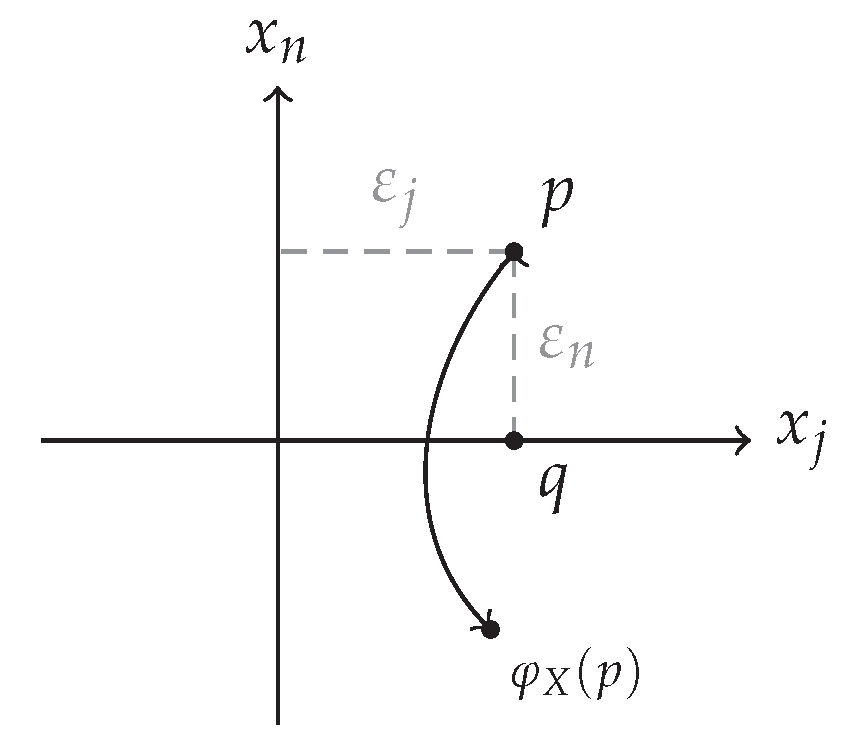
Take a neighborhood V of the origin such that for all for some (it is possible to do this since X is smooth). Fix and consider the points
and
( in the j-th entry and in the n-th entry) with and positives and near enough to zero such that the orbit of p by the field X stays inside V until it touches again the boundary (Figure 5).
Let be the trajectory of X through p:
Then
We have
Since
It follows that
Dividing both sides by , we have
Letting and noticing that
(the last equality is Lemma 15 applied to the tangency point q instead of the origin) and that , we have that
and therefore
On one hand, we have
On the other hand,
Then
and therefore , proving the first equality.
Consider now a point near the origin and let be the trajectory of X through p. Write . Since is a trajectory of X, the last two coordinates of satisfy:
Therefore, the series expansion of the solution is given by
The trajectory touches the boundary when . It occurs at the time
So that, touches at the point
Thus
and therefore
This completes the proof. □
Finally, we prove Lemma 3.
Proof
(Proof of Lemma 3). Consider as in conditions of Lemma 3. We may write
with and . Define as
where is the identity matrix. Then
Define and . By Lemma 16, we have with
(Remember that ). There exists an such that, for all , the matrix is hyperbolic. When , the eigenvalues of whose real part is equal to zero, now have negative real part in and when , they have positive real part in . Consequently, the maps cannot be topologically equivalent for and and therefore, by Lemma 4, the perturbations for cannot be -equivalents to those with . Then it follows that Z is not structurally stable, as we want to demonstrate. □
The proof of this lemma concludes the proof of Theorem 1.
8. Normal Forms
We now prove Theorem 2.
Proof
(Proof of Theorem 2). The fields given in Theorem 2 are structurally stable by Lemma 16 and Lemmas 1 and 2.
If is structurally stable then, by Theorem 1, Z must belong either to the regular or to the singular case. In the regular case, and are conjugate to (8), therefore Z and are -equivalent and we are done. In the singular case, Let be written in the following form
with hyperbolic, and . Let be the field
Define the family of systems
All systems are refractive and for all with A given by Lemma 16 not depending on t.
If were not conjugate to , there would exist a such that is not structurally stable on . This contradicts Theorem 1 and therefore is conjugate to and, by Lemma 4, Z is -equivalent to . □
References
- Brogan, W. Modern Control Theory; Prentice Hall, 1991. [Google Scholar]
- Wang, D.; Luo, S.; Li, W. Global Dynamic Analysis of a Discontinuous Infectious Disease System with Two Thresholds. Internat. J. Bifur. Chaos Appl. Sci. Engrg. 2022, 32, 2250215. [Google Scholar] [CrossRef]
- Filippov, A. Differential Equations With Discontinuous Righthand Sides; Mathematics and its Aplications; Springer Netherlands, 1988. [Google Scholar]
- Guardia, M.; Seara, T.; Teixeira, M. Generic bifurcations of low codimension of planar Filippov systems. J. Differential Equations 2011, 250, 1967–2023. [Google Scholar] [CrossRef]
- Ekeland, I. Discontinuités de champs hamiltoniens et existence de solutions optimales en calcul des variations. Publ. Math. Inst. Hautes Etudes Sci. 1977, 5–32. [Google Scholar] [CrossRef]
- Klok, F. Broken solutions of homogeneous variational problems. J. Differential Equations 1984, 55, 101–134. [Google Scholar] [CrossRef]
- Hogan, S. On the Dynamics of Rigid-Block Motion Under Harmonic Forcing. Proc. R. Soc. Lond. A 1989, 425, 441–476. [Google Scholar] [CrossRef]
- Spanos, P.; Koh, A. Rocking of Rigid Blocks Due to Harmonic Shaking. J. Eng. Mech. 1984, 110, 1627–1642. [Google Scholar] [CrossRef]
- Yim, C.; Chopra, A.; Penzien, J. Rocking Response of Rigid Blocks to Earthquakes. Earthquake Engineering and Structural Dynamics 1980, 8, 565–587. [Google Scholar] [CrossRef]
- Jacquemard, A.; Pereira, W.; Teixeira, M. Generic Singularities of Relay Systems. J. Dyn. Control Syst. 2007, 13, 503–530. [Google Scholar]
- Siller, T. Bifurcações Genéricas em Sistemas Refrativos Elípticos. PhD thesis, Universidade Estadual de Campinas, 2025. [Google Scholar]
- Castro, M.; Martins, R.; Novaes, D. A Note on Vishik’s Normal Form. J. Differential Equations 2021, 281, 442–458. [Google Scholar] [CrossRef]
- Vishik, S. Vector Fields Near the Boundary of a Manifold. Vestinik Moskov. Univ. Ser. I. Mat. Mekh. 1972, 27, 21–28. [Google Scholar]
- Buzzi, C.; Medrado, J.; Teixeira, M. Generic Bifurcation of Refracted Systems. Adv. Math. 2013, 234, 653–666. [Google Scholar] [CrossRef]
- Teixeira, M. Sur la 2-détermination de certains difféomorphismes. C. R. Acad. Sc. Paris 1982, 294, 545–548. [Google Scholar]
- Kress, R. Numerical Analysis; Graduate Texts in Mathematics; Springer New York, 1998. [Google Scholar] [CrossRef]
| 1 | A point is said a crossing point of if . For refractive systems, this is equivalent to . |
| 2 | A function f is said locally Lipschitz at p if there exists some neighborhood V of p such that f restricted to V is Lipschitz. |
Figure 1.
Examples of fold-folds.
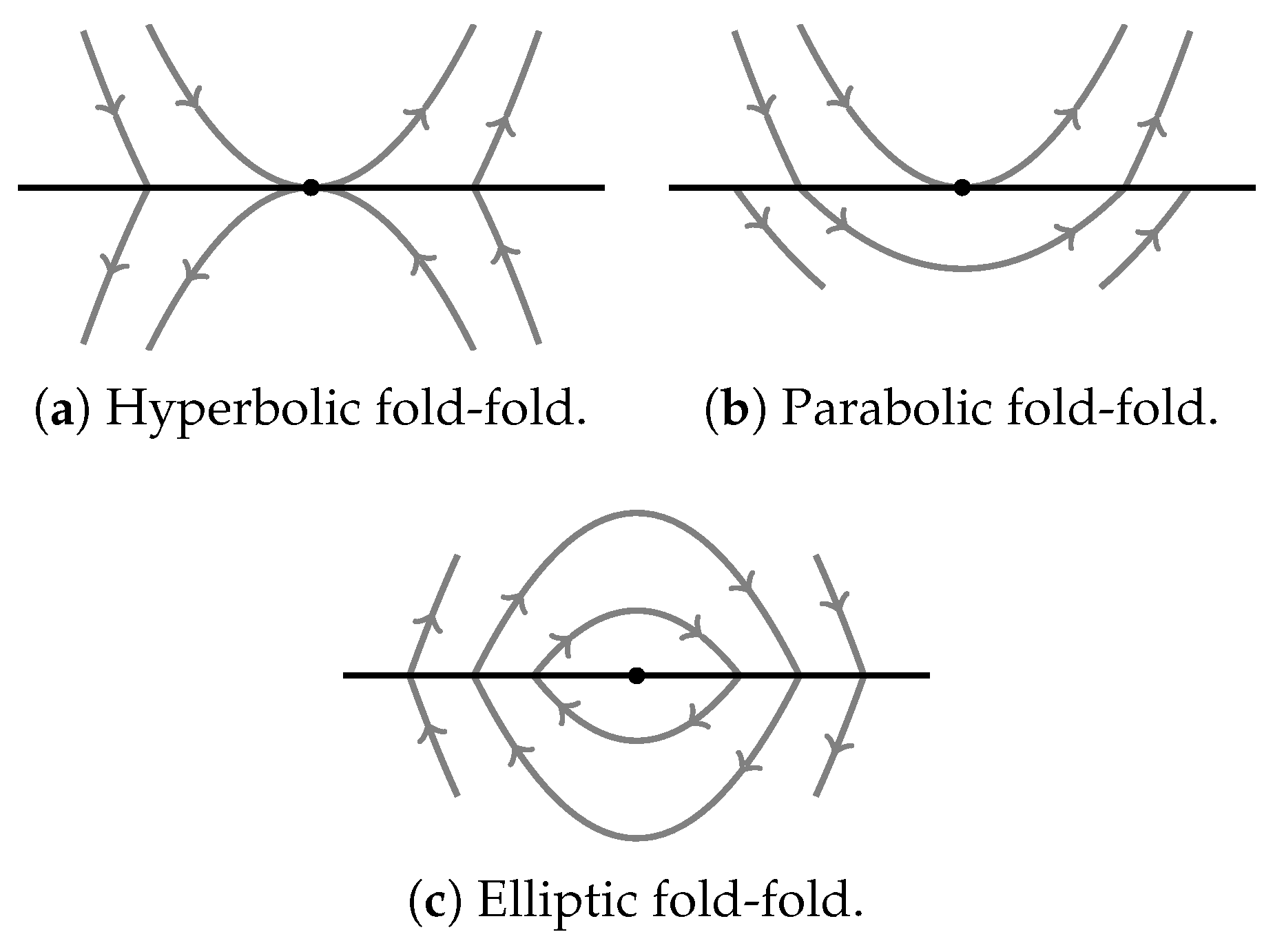
Figure 2.
Involution associated to X. The trajectory of x hits again in the point .
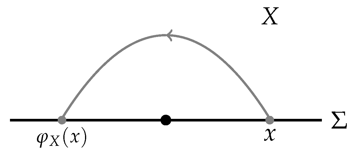
Figure 3.
The construction of Lemma 8.
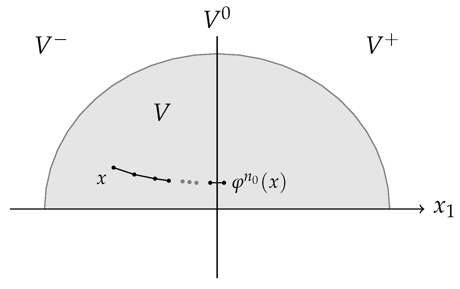
Figure 4.
Regions V, , and .
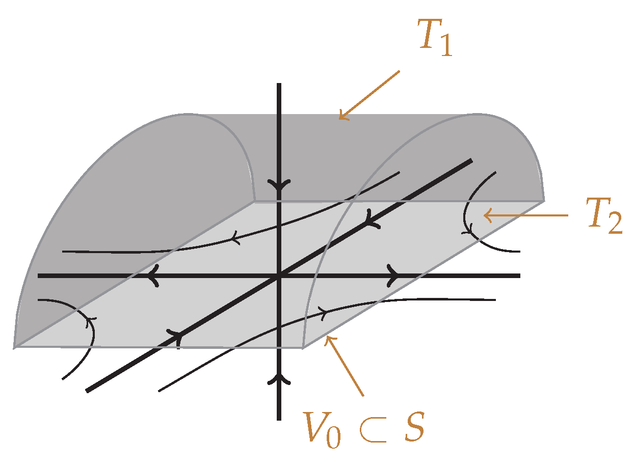
Figure 5.
Construction in the proof of Lemma 16.
Disclaimer/Publisher’s Note: The statements, opinions and data contained in all publications are solely those of the individual author(s) and contributor(s) and not of MDPI and/or the editor(s). MDPI and/or the editor(s) disclaim responsibility for any injury to people or property resulting from any ideas, methods, instructions or products referred to in the content. |
© 2026 by the authors. Licensee MDPI, Basel, Switzerland. This article is an open access article distributed under the terms and conditions of the Creative Commons Attribution (CC BY) license (http://creativecommons.org/licenses/by/4.0/).
Copyright: This open access article is published under a Creative Commons CC BY 4.0 license, which permit the free download, distribution, and reuse, provided that the author and preprint are cited in any reuse.