

Submitted:
26 February 2026
Posted:
27 February 2026
You are already at the latest version
Abstract
Melanoma remains the most lethal form of skin cancer, responsible
for the majority of skin cancer-related fatalities despite its relatively
low incidence \cite{milton2018}. Melanoma can spread to different parts
of the body if it is not identified and treated in its early stages. In
\cite{kumar2021, kumarVatsa2022} previous work on melanoma
classification, the VGG16 architecture of the CNN performed better on the
cancer dataset than any other popular network.
%
The early detection of melanoma by analyzing skin lesion images aims to
enhance early diagnosis and accessibility. However, a significant challenge
arises when incorporating demographic factors as biases in training data,
as they can lead to disparities in model performance across different
populations. These biases often stem from the underrepresentation of
certain demographic groups in medical datasets, leading to lower accuracy
for underserved communities. Such disparities can have serious
consequences, including delayed diagnoses and inadequate treatment
recommendations, further increasing healthcare inequities
\cite{dietterich2000}. Therefore, this study examines the effects of
demographic factors such as age, gender, and data scalability on the early
detection of melanoma. It also evaluates and compares two distinct deep
learning approaches for classifying melanoma from dermoscopic images and
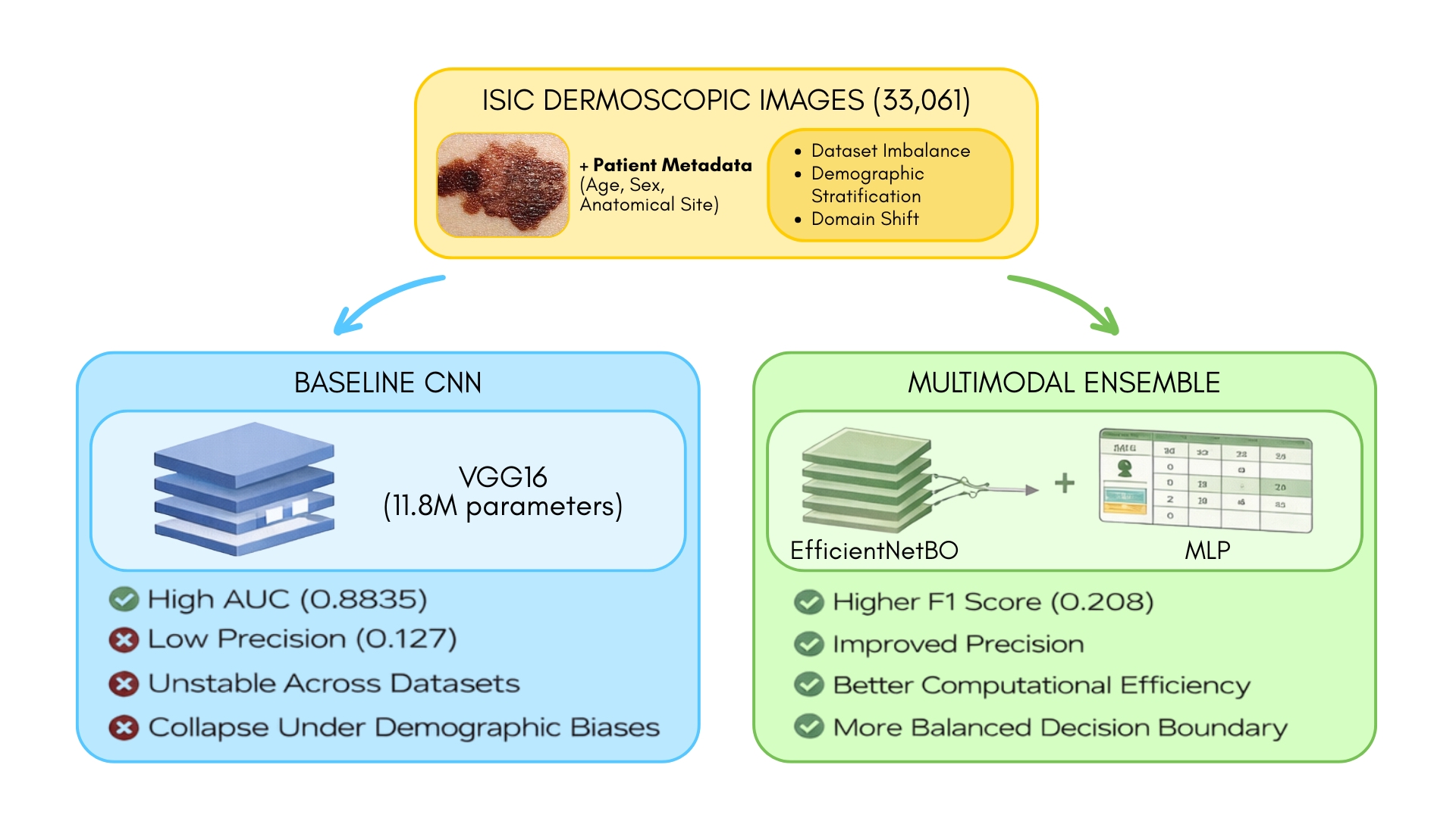
associated patient metadata. The first experiment establishes a baseline
using a VGG-16 convolutional neural network (CNN) trained via transfer
learning. The second, expanded experiment introduces a novel multimodal
ensemble model that synergistically combines an EfficientNetB0 CNN with a
Multi-Layer Perceptron (MLP) to process both image and tabular data
concurrently.
Keywords:
skin cancer
; melanoma
; classification
; CNN
; VGG16
; ensemble
; performance Analysis
1. Introduction
Melanoma is one of the most dangerous types of skin cancer. Although it is less common than other types of skin cancer, it spreads rapidly. It develops in the cells (melanocytes) that produce melanin. The exact cause of the disease is not clear, but it is known that exposure to ultraviolet radiation from sunlight or other sources increases the risk of developing melanoma. The aggressive nature of melanoma, characterized by rapid metastasis, shows the critical importance of early detection. When diagnosed at localized stages, survival rates exceed 95%, but this plummets below 25% once the cancer spreads [10,13]. Traditional diagnostic approaches relying on visual inspection and biopsy suffer from subjectivity, with studies showing dermatologist accuracy ranging between 60-90% [7,22]. This diagnostic variability, combined with global shortages of specialists, creates significant barriers to equitable access to healthcare.
Cancer cells can appear on the skin as a mole from birth or as a result of skin damage [9]. Melanoma can spread to different parts of the body (eyes, ears, gingiva of the upper jaw, tongue, lips, etc.) if it is not identified and treated in its early stages. It most commonly occurs on the chest and legs for men and primarily on the legs for women [9]. Additionally, the occurrence of melanoma has increased by 4-5% in predominantly fair-skinned populations in Europe and America [7,13].
Historically, limited computing power and small datasets constrained early melanoma detection efforts. Today, advances in deep learning and larger dermoscopic datasets have substantially improved performance, with CNNs achieving dermatologist-level accuracy in controlled settings [12,23]. However, recent advancements in artificial intelligence have demonstrated considerable potential in addressing these challenges. Convolutional Neural Networks (CNNs) have achieved diagnostic performance comparable to board-certified dermatologists by automating the analysis of dermoscopic features [10]). Transfer learning approaches using pre-trained models, such as VGG16, have proven particularly effective, outperforming traditional machine learning methods in melanoma classification tasks [8]. Additionally, significant challenges persist, including class imbalance in training datasets and limited generalizability across diverse patient demographics. The International Skin Imaging Collaboration (ISIC) dataset, although comprehensive, contains fewer than 2% malignant samples in some subsets, which may bias model performance [12,20].
Furthermore, ensemble modeling has recently been seen as a powerful tool in machine learning, where multiple models are combined to improve performance, robustness, and generalization compared to any single model. This approach is particularly valuable in complex and high-stakes domains like healthcare, where the consequences of misclassification can be severe. In our previous research, neural networks were used to detect melanoma by analyzing skin lesion images to enhance early diagnosis and accessibility. However, a significant challenge arises when incorporating demographic factors such as race and gender, as biases in training data can lead to disparities in model performance across different populations. These biases often stem from the underrepresentation of certain demographic groups in medical datasets, leading to lower accuracy for underserved communities. Such disparities can have serious consequences, including delayed diagnoses and inadequate treatment recommendations, further increasing healthcare inequities [15,18,19,20,21].
This study builds upon established CNN architectures while introducing novel methodological improvements. By implementing an approach that combines VGG16 with optimized fully connected layers and demographic stratification, we address critical limitations in current systems. The research utilizes a substantial dataset of dermoscopic images from ISIC, carefully balanced and segmented by gender and race to account for known epidemiological variations in melanoma presentation [11,21]. Through rigorous evaluation using AUC-ROC, F1-scores, and sensitivity-specificity analysis, we demonstrate significant improvements over existing benchmarks while maintaining clinical interpretability. The ultimate goal is to develop a scalable diagnostic tool that reduces reliance on invasive procedures and expands access to expert-level skin cancer screening. Therefore, this study examines the effects of demographic factors such as age, gender, and data scalability on the early detection of melanoma. It extends [8]’s previous findings. It classifies malignant and benign images using CNN’s VGG16 and multimodal ensemble model that synergistically combines an EfficientNetB0 CNN with a Multi-Layer Perceptron (MLP) architecture under diverse cases.
This paper is organized into sections, where Section 1 explains the fundamental reasons and available statistics on melanoma skin cancer patients, as introduced in the introduction. Furthermore, the available findings of others are briefly described in Section 2, Background. Section 3 provides the datasets and their statistical significance related to this study, as outlined in the Materials and Methods. The corresponding findings and their discussions are presented in Section 4 of the Results and Discussion section. Finally, Section 5 concludes with the findings of the experiments.
2. Background
Artificial intelligence has had a widespread impact, and its applications have reached multiple domains. As research continues to flourish, novel techniques are proving to be more efficient and effective. The medical industry is no exception, and state-of-the-art medical image classification techniques have reached, and in some cases, even surpassed human capabilities.
The application of deep learning to medical image analysis has revolutionized dermatological diagnostics in recent years. CNNs have emerged as the dominant architecture due to their ability to automatically extract hierarchical features from dermoscopic images without manual feature engineering [10]. This capability proves particularly valuable in melanoma detection, where subtle variations in lesion morphology require sophisticated pattern recognition. Transfer learning techniques, where models pretrained on large datasets like ImageNet are fine-tuned for medical applications, have addressed historical challenges of limited labeled medical data [8]. For instance, the VGG16 architecture has demonstrated exceptional performance in skin lesion classification, achieving superior accuracy compared to shallower networks when adapted through careful layer freezing and retraining strategies.
Despite these advances, significant hurdles remain in developing clinically robust systems. Dataset imbalance represents a persistent challenge, with malignant samples often underrepresented in training collections [12]. This imbalance can lead to models with high specificity but poor sensitivity—a dangerous combination in medical diagnostics, where false negatives carry severe consequences. Recent work has employed various techniques to mitigate this issue, including the generation of synthetic data through Generative Adversarial Networks and the strategic oversampling of minority classes [22]. Additionally, the integration of patient metadata such as age, gender, and lesion location has shown promise in improving model performance, reflecting known epidemiological patterns of melanoma presentation [9].
The clinical implementation of these technologies has begun to show a measurable impact. Several studies have documented how AI-assisted diagnosis can improve accuracy among both specialists and general practitioners [11,20]. In some cases, the combination of algorithmic analysis with clinician expertise has achieved diagnostic performance that surpasses that of the approach used independently. However, concerns remain regarding model interpretability and the need for systems that provide not just predictions but clinically actionable insights [13]. As the field progresses, the focus has shifted from pure accuracy metrics to developing robust, fair, and deployable systems that can integrate seamlessly into diverse healthcare environments.
In recent years, the increase in computational power coupled with the abundance of data has led to deep learning models becoming more efficient. The most common algorithms used in medical image classification are Convolutional Neural Networks (CNNs).
CNNs are a type of artificial neural network that is focused on the classification of images [10,20,22]. The primary limitation of artificial neural networks in handling image datasets is that the computational complexity increases significantly with large amounts of data. The training becomes exceedingly slow and leads to poor performance. Convolutional neural networks are different from traditional neural networks in that each neuron within any given layer will only connect to a small region of the layer preceding it [10]. This means that the overall complexity of computation is greatly reduced, and the entire network performs better. The architecture consists of three main layers, which may be repeated: the convolutional layer, the pooling layer, and the fully connected layer.
Figure 1 illustrates the main functionality of the three layers of the CNN. The first layer is the convolutional layer, which calculates the output of neurons connected to local regions. Next, the pooling layer down-samples the neurons, further reducing the neurons in that activation. Finally, the fully connected layer performs the same functions as the artificial neural networks do. Thus, convolutional neural networks can perform image classification with lower computational complexity while still achieving high accuracy.
Since pre-trained CNNs have developed skills in tasks like pattern recognition and edge detection, transfer learning can fine-tune the pre-trained model for more specific tasks. VGG16 is a deep convolutional neural network that is considered one of the best computer vision models to date. The VGG16 model comprises multiple convolutional, pooling, and fully connected layers that enable state-of-the-art edge detection and pattern recognition. This architecture achieved the highest score on the ImageNet dataset. The ImageNet Large Scale Visual Recognition Challenge (ILSVRC) focuses on evaluating models on object detection and image classification. The dataset is open source and available for public access. In previous work performed by [8], it was observed that a model using the pre-trained weights of VGG16 performed better on the cancer dataset than any other popular network.
Significant work has been conducted in image classification for cancerous cells. [11] produced work that showed the effect that neural networks have on cancer classification. They used a novel deep learning approach to the problem by using multiple CNN models. The achieved AUC (area under ROC curve) was 0.72. In [12], created a model that can recognize skin lesions and detect the presence of cancerous tissues. He applied CNNs with transfer learning in his approach, which is similar to our approach. [22] viewed Artificial Intelligence (AI) as an ancillary tool for professionals to aid them in their decision-making. They used multiple deep learning algorithms to create an effective model. 73.9% of non-medical professionals changed answers from non-malignancy to malignancy, increasing their accuracy.
The significant difference between CNN and other ANN algorithms is that CNNs allow to implement features specific to images in the architecture itself, which makes it optimal for image detection. CNNs enable the use of partially connected layers, which improves overall performance metrics and reduces the total number of parameters required.
Ensemble methods offer a promising solution to these challenges by combining diverse models to mitigate the limitations of individual approaches. For instance, the strength of an ensemble depends on the diversity of its models and their ability to correct each other’s errors, which is particularly relevant in melanoma detection [16]. Lesions can vary significantly in appearance based on factors like body location and skin type. For example, acral lentiginous melanoma, a rarer but aggressive form of melanoma, is more commonly found on the palms, soles, and under the nails, particularly in darker-skinned individuals. By training an ensemble of models to classify lesions not only by malignancy but also by location, we can better capture the nuanced ways melanoma presents across diverse populations. This approach could enhance early detection strategies and enable more personalized treatment recommendations [17,18].
Moreover, ensemble methods have shown that combining models can improve both predictive accuracy and uncertainty estimation, making them more reliable for critical applications like medical diagnosis [18]. In the context of melanoma detection, this means that ensembles could not only improve diagnostic accuracy but also provide confidence estimates that help healthcare professionals make more informed decisions. Additionally, efficient techniques for training ensembles address the computational challenges often associated with combining multiple models, making them more accessible for real-world applications [18,19]. By utilizing these advancements, we can develop more equitable and effective tools for melanoma detection, ensuring that all populations, regardless of demographic factors, benefit from the latest advancements in machine learning.
3. Materials and Methods
Every year, the International Skin Imaging Collaboration (ISIC) announces contests and competitions aimed at creating new algorithmic techniques for the detection and classification of skin diseases. The dataset used for this research was the public repository of ISIC. This study considered five diverse datasets. The dataset distribution of Dataset 1 through Dataset 5 is illustrated in Figure 2 [1,2,3,4,5,6]. The datasets have been divided into training, testing, and validation, with a 60-20-20 split. The distribution of benign and malignant images in the five datasets has been illustrated in Figure 2(a) for training images, Figure 2(b) for test images, and Figure 2 (c) for validation images. There are significant differences in datasets 1, 4, and 5. Datasets 4 and 5 are the worst combinations for the overall datasets. Dataset 5 exhibits a considerable difference in the number of benign and malignant images, rendering its results unreliable [1,2,3,4,5,6].
Table 1 lists the number of images for the training, test, and validation datasets for datasets 1 through 5 [1,2,3,4,5]. The training dataset comprises 75% of the images, whereas the test and validation datasets contain 12.5% of the total images, except for dataset 5. Dataset 5 comprises 50% of the total images for training and 25% for the test and validation datasets.
Figure 3(a) demonstrates the gender distribution of dataset 1. In contrast, Figure 3(b) and Figure 3(c) show the distribution of males and females versus age for the test and training datasets of dataset 1, respectively. Based on this distribution, the number of images for males and females in different age groups differs between the training and test datasets in dataset1. The lighter hue of bars in Figure 3(c) shows the training dataset and its distribution. Additionally, the darker bars in Figure 3(b) show the distribution of the testing dataset.
The descriptive statistics of the test and training datasets for Dataset 1, broken down by gender, are depicted in Figure 4(b) and Figure 4(c), respectively. Figure 4(a) shows the combined statistical distribution of the male and female datasets for both the test and training sets. Figure 4(b) shows the testing dataset, where most images are of males rather than females. In Figure 4(a), Figure 4(b), and Figure 4(c), the distribution of the data by gender and age is shown. The green triangle inside the boxes shows the mean value of the approximate ages of males and females in dataset 1, and the horizontal line shows us the median age.
In total, dataset 1 contains 33061 dermoscopic images to measure and compare the performance of CNN. Each image was preprocessed before feeding it into the neural network. These images are converted to grayscale and further normalized.
The VGG16 of Convolutional Neural Network was used as the base classification model for this study. In previous work [8], a conclusion was reached that a CNN architecture using the VGG16 performs better on the melanoma dataset than other popular image classification networks. For this experiment, we added a fully connected layer to the VGG16 architecture to custom-train the weights as per our dataset.
Moreover, the hyperparameters are tuned, and improvements in performance metrics, including accuracy, F1 scores, and the area under the ROC curve, are observed. Additionally, various activation functions, such as ReLU, sigmoid, and SoftMax, are employed to achieve improved values of the performance metrics. The loss function used in this model uses binary cross-entropy. This was chosen to solve a binary classification problem (malignant versus benign). The Stochastic Gradient Descent (SGD) function is used to optimize the model.
In this experiment, five different datasets are used to measure the performance metrics, including the F1 score, of the VGG16 architecture of CNN. To determine the best combination of datasets and corresponding F1 score, the model is trained on Dataset 1 and tested on all five datasets (Dataset 1 through Dataset 5) [1,2,3,4,5] separately for a fair measure. To further improve the model’s performance by fine-tuning its hyperparameters, the datasets are divided based on gender and race. This is done to find the correlation between the gender and race of a person with melanoma identification [14].
Additionally, a second experiment builds upon the expanded experiment, introducing a novel multimodal ensemble model that synergistically combines an EfficientNetB0 CNN with a Multi-Layer Perceptron (MLP) to process both image and tabular data concurrently. It utilizes the images from Dataset 1 [1,6], which comprises dermoscopic images in JPEG format with a standard resolution of 256x256 pixels. Accompanying the image data is a CSV file containing tabular metadata for each case. The key features considers in this study which includes patient-level information (patient_id, sex, and age_approx), skin lesion information (anatom_site_general_challenge (the anatomical location of the lesion)) and target labels (target, a binary indicator where 1 represents malignant melanoma and 0 signifies a benign lesion) [18].
A comprehensive data preprocessing pipeline was developed for the new ensemble model. The tabular metadata went through several transformation steps for the MLP model:
- Categorical Encoding: To handle non-numeric features, one-hot encoding was applied to the anatomical location of the lesion and patient_id columns. This converts each category into a new binary feature, preventing the model from assuming an ordinal relationship between the categories.
- Binary Mapping: The sex feature was mapped to numerical values (male : 1, female : 0)
- Handle Missing Values: Missing values in the sex and age_approx columns were imputed with -1 and 0, respectively, to ensure data integrity.
- The age_approx feature was normalized by dividing by its maximum value, scaling the data to a range between 0 and 1.
After these steps, irrelevant columns (diagnos, benign_malignant, etc.) were dropped, resulting in a final feature vector of 2064 dimensions for each patient case.
The images were loaded with OpenCV and converted from the BGR color space to RGB to match the standard convention for models pre-trained on ImageNet. Afterwards, for the VGG-16 baseline model, images were resized to 128x128 pixels. For the multimodal ensemble model, a higher resolution of 256x256 pixels is used.
Thereafter, the complete dataset was partitioned into training and testing sets using a . This resulted in samples for the training set and samples for the test set. Additionally, of the training data was reserved for validation.
Moreover, to enhance classification performance by leveraging patient metadata, a multimodal ensemble architecture was implemented. The model consists of two parallel sub-networks that process the image and tabular data independently before combining their outputs for a final prediction.
The proposed ensemble model integrates an image-processing CNN and a tabular-data processing MLP.
- Image Sub-network (CNN): An EfficientNetB0 model, pre-trained on ImageNet, was employed as the backbone. The convolutional base was used for feature extraction, and the output of the base was passed through a GlobalAveragePooling2D layer to reduce the spatial dimensions into a feature vector, which was then fed into a Dense layer with four output units. This architecture fine-tunes the EfficientNetB0 architecture for our specific task.
- Tabular Sub-network (MLP): A simple MLP was used to process the 2064-dimensional tabular feature vectors. It consists of an input layer, a Dense layer with eight neurons and ReLU activation, and a final Dense layer with four neurons and ReLU activation.
- Fusion and Classification: The 4-unit output tensors from both the CNN and MLP sub-networks were concatenated along their feature axis, resulting in a combined 8-unit feature vector. This fused vector was then passed through a final two-layer classifier: a Dense layer with four units (ReLU activation) followed by the output Dense layer with a single neuron and a sigmoid activation function, which produces the final probability of malignancy.
A key advantage of this architecture is its efficiency. The entire ensemble model contains only 4.03 million trainable parameters, nearly a third of the VGG-16 baseline (∼ 11.8 million parameters), despite processing higher-resolution images and an additional stream of tabular data. A diagram of the whole model architecture is shown in Figure 5.
The model is implemented in Python using TensorFlow. The model was compiled with the Adam optimizer and binary cross-entropy loss function. To address the severe class imbalance in the dataset, class weights were applied during training, assigning a weight of 50 to the minority (malignant) class and a weight of 1 to the majority (benign) class. The model was trained with a batch size of 128. Early stopping was employed, monitoring the validation F1 score with a patience of 20. The training process was halted after 26 epochs as the model’s performance on the validation set ceased to improve.
4. Results and Discussions
The CNN’s VGG 16 model architecture includes thirteen convolutional layers, five pooling layers, and three dense layers. The model was trained for 503 epochs, and training was stopped early after 26 epochs since it converged. This model uses a sigmoidal activation function and the SGD optimizer.
When the VGG16 model is trained on Dataset 1 and evaluated across datasets Dataset 1 through Dataset 5, the model performance metric values are listed in Table 2 and illustrated in Figure 6. It performed best on its test dataset (accuracy: 89.58%, recall: 0.5010) but exhibited a sharp decline in generalization to external datasets. On the balanced Dataset 2, performance dropped to near-random levels (accuracy: 49.03%, ROC AUC: 0.4932), likely due to the interaction between class weighting during training and the balanced class distribution of Dataset 2. Interestingly, the model achieved relatively strong performance on Dataset 3 (accuracy: 77.90%, F1-score: 0.7535), suggesting partial feature transferability when the domain characteristics were more aligned with Dataset 1. However, on Dataset 4 and Dataset 5, recall collapsed (0.1749 and 0.0000, respectively), with the model entirely failing to detect malignant samples in Dataset 5. These results highlight that while VGG16 trained on Dataset 1 can capture features useful for some external datasets, its cross-dataset generalization is highly inconsistent and sensitive to dataset-specific characteristics such as class imbalance and image domain differences. Additionally, if there are more images or a balanced dataset, the model might perform even better on other datasets as well.
When the VGG16 model is trained on Dataset 2 and evaluated across datasets Dataset 1 through Dataset 5, the model performance metric values are listed in Table 3 and illustrated in Figure 7. The VGG16 model demonstrated excellent in-domain performance on Dataset 2 (accuracy: 88.52%, recall: 0.8974, F1-score: 0.8859), confirming its ability to classify malignant and benign cases within a balanced dataset effectively. However, performance degraded substantially on external datasets. On Dataset 1, accuracy remained relatively high (88.28%), but recall fell sharply to 0.0782, suggesting a strong bias toward benign predictions in this heavily imbalanced dataset. On Dataset 3, the model’s accuracy dropped to 55.10%, with modest recall (0.1433), indicating difficulty transferring to a dataset with similar class proportions but distinct domain characteristics. Dataset 4 exhibited slightly better overall accuracy (77.17%), yet malignant detection remained minimal (recall: 0.0296). On Dataset 5, the model achieved a very high apparent accuracy (95.53%) but failed to identify malignant cases (recall: 0.0000), reflecting a collapse to predicting only the majority class. These results indicate that while training on a balanced dataset like Dataset 2 improves within-domain classification, it does not guarantee robust cross-dataset generalization, especially in the presence of severe class imbalance or domain shift.
When the VGG16 model is trained on Dataset 4 and evaluated across datasets Dataset 1 through Dataset 5, the model performance metric values are listed in Table 4 and illustrated in Figure 8. This VGG16 model exhibited poor malignant case detection both in-domain (Dataset 4) and across external datasets. On its test split (Dataset 4), overall accuracy was moderate (83.26%), but recall and F1-score were both 0.0000, indicating a complete failure to identify malignant samples despite a relatively high ROC value (0.7316). On Dataset 1, accuracy was deceptively high (97.76%), but recall remained near zero (0.0068), reflecting a strong bias toward benign predictions in this heavily imbalanced dataset. Performance on the balanced datasets was similarly weak: Dataset 2 and Dataset 3 achieved accuracies of 49.14% and 53.01%, respectively, but with minimal recall (0.0130 and 0.0251, respectively), leading to very low F1-scores. On Dataset 5, the model reached its highest apparent accuracy (98.10%) but again failed to detect any malignant cases (recall: 0.0000). These results suggest that training on Dataset 4, a relatively small and imbalanced dataset, led to severe overfitting and an inability to generalize, with the model effectively collapsing into a benign-only prediction strategy across all domains.
When the VGG16 model is trained on Dataset 3 and evaluated across datasets Dataset 1 through Dataset 5, the model performance metric values are listed in Table 5 and illustrated in Figure 9. This VGG16 model achieved strong in-domain (Dataset 3) performance (accuracy: 92.88%, recall: 0.9303, F1-score: 0.9252, ROC: 0.9821), reflecting effective learning within this relatively balanced dataset. However, its generalization to other datasets varied significantly. On Dataset 1, the model achieved high accuracy (94.77%) but with a low recall of 0.1228, suggesting a bias toward benign predictions in this heavily imbalanced dataset. On Dataset 2, performance degraded sharply (accuracy: 38.84%, recall: 0.2633, F1-score: 0.2977), indicating difficulty transferring to a dataset with similar class proportions but differing visual or annotation characteristics. Testing on Dataset 4 resulted in moderate accuracy (62.83%) but poor malignant detection (recall: 0.2661), and on Dataset 5, although overall accuracy was 71.88%, the model completely failed to identify malignant samples (recall: 0.0000). These findings suggest that while training on Dataset 3 produces a model capable of excellent within-dataset performance, it struggles with external datasets, particularly those with severe imbalance or substantial domain differences, highlighting the persistent challenge of cross-dataset generalization in melanoma classification.
When the VGG16 model is trained on Dataset 5 and evaluated across datasets Dataset 1 through Dataset 5, the model performance metric values are listed in Table 6 and illustrated in Figure 10. This VGG16 model tests across Dataset 1 through Dataset 5, and the VGG16 model showed a complete collapse in malignant case detection. Even on its test split (Dataset 5), the model achieved perfect accuracy (100%) but a recall of 0.0000 and F1-score of 0.0000, indicating that it predicted only the majority (benign) class. This behavior persisted across all external datasets: Dataset 1 (accuracy: 98.24%), Dataset 2 (50.00%), Dataset 3 (52.06%), and Dataset 4 (80.50%) all exhibited zero recall and F1-scores despite superficially high or moderate accuracy values. These results suggest that training on Dataset 5, a small and highly imbalanced dataset, led to extreme overfitting and a trivial decision boundary biased toward benign classifications. Consequently, the model failed to generalize meaningfully to any dataset, including its own, underscoring the limitations of using small, skewed datasets for training deep learning models in melanoma detection.
Subsequently, the experiment conducts a subset analysis using only the male and female cohorts separately from Dataset 1. Using these cohorts, we then repeat the procedure, to test for these gender differences.
When the VGG16 model is trained on the female-only cohort of Dataset 1 and evaluated across all other datasets, the VGG16 model achieved high accuracy with images of the same dataset but completely failed to detect malignant cases despite the class weights. The model performance metric values are listed in Table 7 and illustrated in Figure 11. The female-only test dataset achieved a classification accuracy of 98.73%, but the F1 score of zero indicates that it only predicted the benign class. Testing on the male-only cohort of Dataset 1, the VGG16 model produces similar results. On Dataset 2, accuracy is near chance at 49.79%, with near-zero recall and a very low F1-score. This suggests the pattern of guessing benign did not translate to more balanced datasets. Dataset 3 and Dataset 4 produce moderate accuracies but still have a very low recall. This highlights how class imbalance in training data can lead to less transfer when other datasets have different distributions.
When the VGG16 model is trained on the male-only cohort of Dataset 1 and evaluated across all other datasets, the VGG16 model showed similar behavior to the female-trained model, which includes high in-cohort accuracy but a complete failure to detect malignant cases. This likely reflects the already limited number of malignant samples in Dataset 1 being further reduced by gender-based stratification, leaving the model with insufficient examples to learn meaningful malignant features. The model performance metric values are listed in Table 8 and illustrated in Figure 12.
The performance of the baseline VGG16 and the proposed multimodal ensemble model is evaluated on the held-out test set using performance metrics, which include Loss, Binary Accuracy, AUC, Precision, Recall, and F1 Score. The evaluation results for both models are presented in Table 9 and illustrated in Figure 13.
The results (Table 9) demonstrate that the multimodal ensemble model represents a more balanced and efficient solution than the VGG-16 baseline, achieving a superior F1 Score with significantly fewer computational resources.

Table 9.
VGG16 versus Ensemble Model Comparison
| Datasets Metrics |
VGG16 Model | Ensemble Model |
|---|---|---|
| Loss | 0.2407 | 0.2755 |
| Binary Accuracy | 0.8958 | 0.9570 |
| AUC | 0.8835 | 0.6866 |
| Precision | 0.1270 | 0.1898 |
| Recall | 0.5010 | 0.2323 |
| F1 Score | 0.1926 | 0.2080 |
Table 10.
Hyperparameter values of VGG16 and Ensemble Model
| Models Model Stats. |
VGG16 Model | Ensemble Model |
|---|---|---|
| Trainable Parameter | ||
| Batch Size | 64 | 128 |
| Image Size | 128 | 256 |
The VGG-16 model established a firm baseline in two key areas: AUC (0.8835) and Recall (0.5010). Its high recall indicates it is sensitive, correctly identifying over 50% of malignant cases. However, this sensitivity comes at a severe cost to precision (0.1270), meaning it generated a very high number of false positives. In contrast, the multimodal ensemble model shows marked improvements in several areas. Its F1 Score of 0.2080 surpasses the baseline, indicating a better balance between precision and recall. This was achieved while using a more computationally efficient architecture (4.0M vs. 11.8M parameters) and leveraging higher-resolution input images (256x256 vs. 128x128). The model’s high binary accuracy (0.9570) is notable, although primarily driven by its correct classification of the abundant benign samples.
A critical point of divergence remains the AUC. The VGG-16’s high AUC suggests it is fundamentally better at distinguishing between the classes across all decision thresholds. The ensemble model’s lower AUC of 0.6866, while an improvement over initial training runs, indicates that its probability scores are not as well-calibrated for separating the classes. It achieves a good operating point (as shown by the F1-score) but lacks the overall discriminative power of the VGG-16. Thus, the ensemble model has more clearly identified characteristics of malignant images.
5. Conclusions
This study investigated two critical challenges in the deep learning-based classification of melanoma: the brittleness of models against domain shift and the potential for multimodal architectures to improve performance. Our first experiment systematically revealed the profound limitations of a standard VGG-16 model in cross-dataset generalization. When trained on one data source and tested on others, the model’s performance was highly inconsistent and often collapsed entirely, particularly in its ability to recall malignant cases. This failure occurred regardless of whether the training data was balanced or imbalanced, underscoring that models can easily overfit to dataset-specific visual characteristics and are not inherently robust enough for deployment across varied clinical environments.
Building on these findings, our second experiment demonstrated that a more sophisticated approach—a multimodal ensemble model combining an EfficientNetB0 CNN with an MLP for patient metadata—can offer a more balanced and computationally efficient solution. This ensemble model surpassed the VGG-16 baseline in F1-score and precision, proving that integrating non-image data provides valuable context that helps create a more robust decision boundary. Critically, it achieved this with nearly a third of the trainable parameters, highlighting a path toward more effective and scalable models. The success of this approach suggests that overcoming the domain shift problem highlighted in our first experiment may require not just better training strategies, but architectures that are less reliant on visual features alone.
Despite its advantages, our proposed ensemble model is not without its own limitations. Its significantly lower AUC and recall compared to the VGG-16 baseline indicate that while its specific decision threshold is well-balanced (leading to a higher F1-score), its fundamental ability to rank cases by their probability of malignancy is still suboptimal. This trade-off between a high-recall, low-precision “screening” model (VGG-16) and a balanced, higher-precision “diagnostic aid” model (the ensemble) is a key finding of this work.
Future research should focus on merging the strengths of both approaches. A crucial next step is to explore whether the multimodal ensemble architecture, when trained on an aggregation of diverse datasets, can overcome the generalization failures seen in the first experiment. Additionally, implementing advanced loss functions like focal loss or exploring more sophisticated data fusion mechanisms could help elevate the ensemble model’s AUC and recall, potentially creating a single model that is not only balanced and efficient but also possesses the high sensitivity and robust generalization required for real-world clinical application.
Author Contributions
All authors contributed equally in this manuscript.
Funding
This research has not been supported by external funding.
Informed Consent Statement
Humans has not been involved in this rearch experiments.
DURC Statement
Current research is limited to the Early detection of Melanoma Skin Cancer, which is beneficial in early detection through the demoscopic images and does not pose a threat to public health or national security. Authors acknowledge the dual-use potential of the research involving image analysis using neural network based algorithms and confirm that all necessary precautions have been taken to prevent potential misuse. As an ethical responsibility, authors strictly adhere to relevant national and international laws about DURC. Authors advocate for responsible deployment, ethical considerations, regulatory compliance, and transparent reporting to mitigate misuse risks and foster beneficial outcomes.
Acknowledgments
We gratefully acknowledge the support of the Research Release Time and Grant-in-Aid of Gildart Haase School of Computer Sciences & Engineering, Fairleigh Dickinson University, Teaneck, New Jersey 07666, USA. Additionally, we greatly appreciate the support of other members of Deep Chain (DC) Lab
Conflicts of Interest
Declare conflicts of interest or state “The authors declare no conflicts of interest.” Authors must identify and declare any personal circumstances or interest that may be perceived as inappropriately influencing the representation or interpretation of reported research results. Any role of the funders in the design of the study; in the collection, analyses or interpretation of data; in the writing of the manuscript; or in the decision to publish the results must be declared in this section. If there is no role, please state “The funders had no role in the design of the study; in the collection, analyses, or interpretation of data; in the writing of the manuscript; or in the decision to publish the results”.
References
- Dataset 1. Available online: https://www.kaggle.com/competitions/siim-isic-melanoma-classification/data.
- Dataset 2. Available online: https://www.kaggle.com/datasets/drscarlat/melanoma.
- Dataset 3. Available online: https://www.kaggle.com/datasets/hasnainjaved/melanoma-skin-cancer-dataset-of-10000-images.
- Dataset 4. Available online: https://www.kaggle.com/datasets/wanderdust/skin-lesion-analysis-toward-melanoma-detection?select=skin-lesions.
- Dataset 5. Available online: https://www.kaggle.com/datasets/nodoubttome/skin-cancer9-classesisic.
- Dataset 6. Available online: https://challenge.isic-archive.com/data/.
- Kaggle Website. Available online: https://www.cancer.org/cancer/melanoma-skin-cancer.html.
- Kumar, A.; Vatsa, A. Untangling Classification Methods for Melanoma Skin Cancer. In Frontiers in Big Data, Data Mining, and Management; 2022; Volume 5. [Google Scholar] [CrossRef]
- Milton, M. A. A. Automated skin lesion classification using ensemble of deep neural networks. in isic 2018: skin lesion analysis towards melanoma detection challenge. in ISIC 2018 (Barcelona) 2018, 225–228. [Google Scholar]
- O’shea, K.; Nash, R. “An Introduction to Convolutional Neural Networks”; 2015. [Google Scholar] [CrossRef]
- Guo, Y.; Ashour, A. Multiple Convolutional Neural Network for Skin Dermoscopic Image Classification. Available online: https://arxiv.org/ftp/arxiv/papers/1807/1807.08114.pdf.
- Chang, H. “Skin cancer reorganization and classification with deep neural network”. Available online: https://arxiv.org/ftp/arxiv/papers/1703/1703.00534.pdf.
- Kosary, Carol L.; Altekruse, Sean F.; Ruhl, Jennifer; Lee, Richard; Dickie, Lois. “Clinical and prognostic factors for melanoma of the skin using SEER registries: collaborative stage data collection system, version 1 and version 2.”. Cancer 2014, 120 Suppl 23, 3807–14. [Google Scholar] [CrossRef] [PubMed]
- Yuan, Tze-An; Lu, Yunxia; Edwards, Karen; Jakowatz, James; Meyskens, Frank L.; Liu-Smith, Feng. “Race-, Age-, and Anatomic Site-Specific Gender Differences in Cutaneous Melanoma Suggest Differential Mechanisms of Early- and Late-Onset Melanoma”. Int. J. Environ. Res. Public Health. [CrossRef]
- Dietterich, T. G. Ensemble Methods in Machine Learning. In Multiple Classifier Systems, MCS 2000. Lecture Notes in Computer Science; Springer: Berlin, Heidelberg.; vol 1857. [CrossRef]
- Breiman, Leo. Random Forests. Available online: https://www.stat.berkeley.edu/~breiman/randomforest2001.pdf.
- Chen, Tianqi; Guestrin, Carlos. “XGBoost: A Scalable Tree Boosting System”. In KDD ’16: Proceedings of the 22nd ACM SIGKDD International Conference on Knowledge Discovery and Data Mining; pp. 785–794. [CrossRef]
- Fort, Stanislav; Hu, Clara Huiyi; Lakshminarayanan, Balaji. “Deep Ensembles: A Loss Landscape Perspective”. Available online: https://openreview.net/forum?id=r1xZAkrFPr.
- Huang, Gao; Li, Yixuan; Pleiss, Geoff; Liu, Zhuang; Hopcroft, John; Weinberger, Kilian. “Snapshot Ensembles: Train 1, get M for free”. 10.48550/arXiv.1704.00109. [CrossRef]
- Vieira, Jonathan; Mendonca, Fábio; Morgado-Dias, Fernando. Deep Learning Approaches for Skin Lesion Detection. Electronics vol. 14(no. 14), 2785, 2025. [CrossRef]
- Ali, R.; Hardie, R. C.; Narayanan Narayanan, B.; De Silva, S. “Deep Learning Ensemble Methods for Skin Lesion Analysis towards Melanoma Detection”. 2019 IEEE National Aerospace and Electronics Conference (NAECON), Dayton, OH, USA, 2019; pp. 311–316. [Google Scholar] [CrossRef]
- Han, Seung Seog; Park, Ilwoo; Chang, Sung Eun; Lim, Woohyung; Kim, Myoung Shin; Park, Gyeong Hun; Chae, Je Byeong; Huh, Chang Hun; Na, Jung-Im. “Augmented Intelligence Dermatology: Deep Neural Networks Empower Medical Professionals in Diagnosing Skin Cancer and Predicting Treatment Options for 134 Skin Disorders”. Journal of Investigative Dermatology 2020, Vil. 140(No. 9), 1753–1761. [Google Scholar] [CrossRef] [PubMed]
- Vatsa, A. SDFS: A Standardization Technique for Nonparametric Analysis. International Journal on Engineering, Science and Technology (IJonEST) 2021, Vol. 3(No. 1), 30–43. Available online: https://ijonest.net/index.php/ijonest/article/view/31. [CrossRef]
Figure 1.
CNN Architecture.
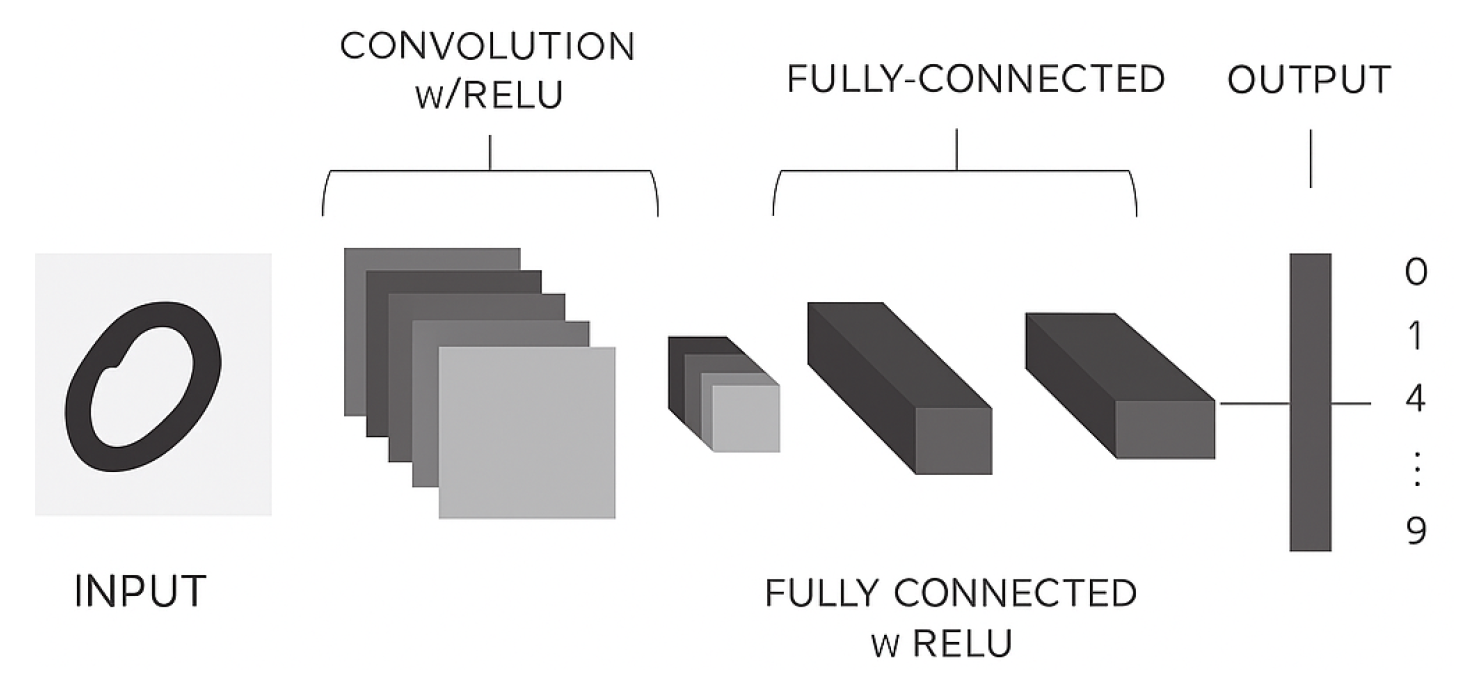
Figure 2.
Distribution of Malignant and Benign images for Datasets 1 through 5.: (a) Training. (b) Test. (c) Validation dataset.
Figure 2.
Distribution of Malignant and Benign images for Datasets 1 through 5.: (a) Training. (b) Test. (c) Validation dataset.
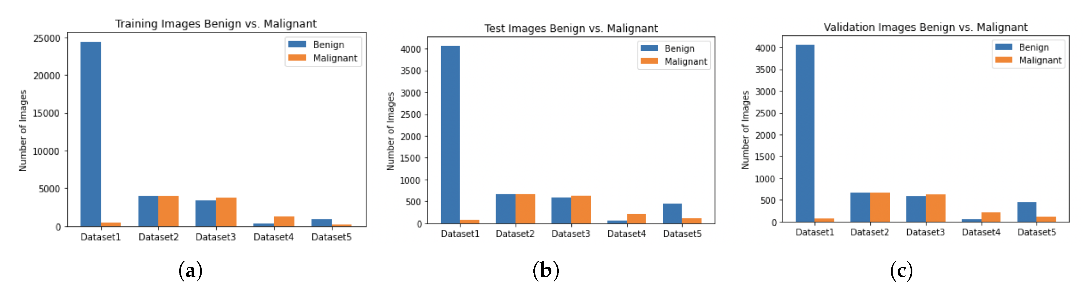
Figure 3.
Distribution of age of males and females in dataset 1.: (a) Dataset 1. (b) Test Dataset. (c) Training Dataset.
Figure 3.
Distribution of age of males and females in dataset 1.: (a) Dataset 1. (b) Test Dataset. (c) Training Dataset.
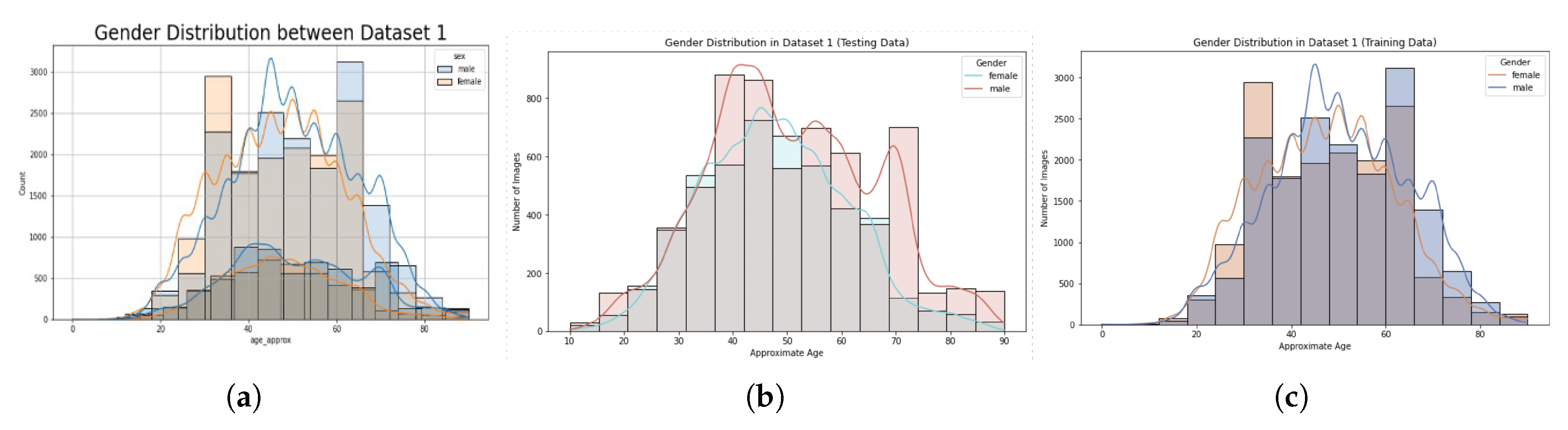
Figure 4.
Descriptive statistics of males and females in dataset 1.: (a) Training and test dataset for male and female corresponding to age. (b) Training and test dataset for male and female corresponding to age. (c) Training dataset age and gender.
Figure 4.
Descriptive statistics of males and females in dataset 1.: (a) Training and test dataset for male and female corresponding to age. (b) Training and test dataset for male and female corresponding to age. (c) Training dataset age and gender.
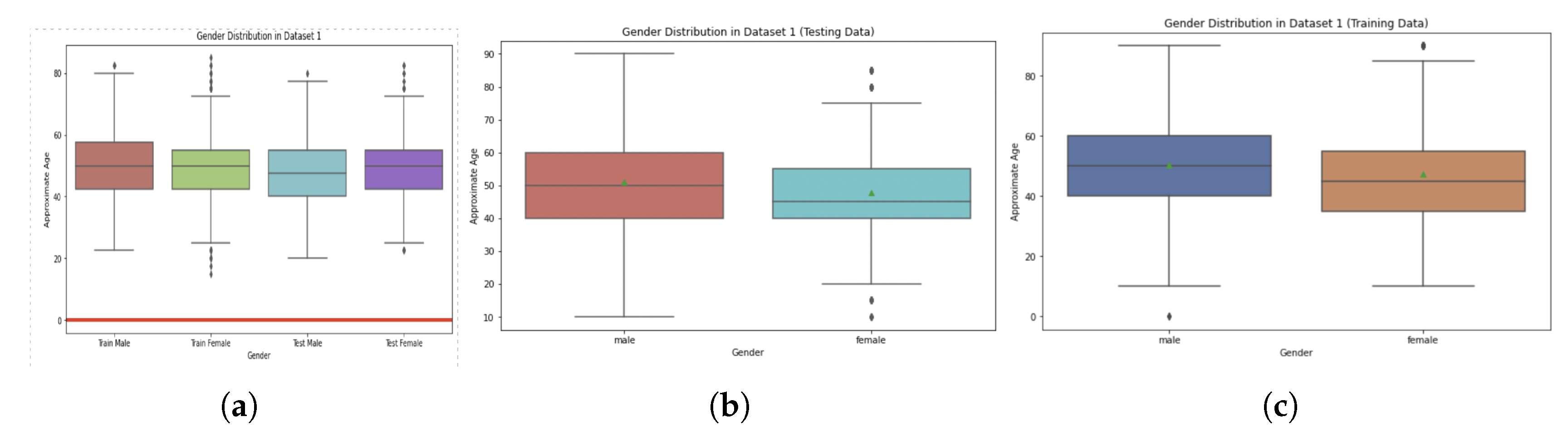
Figure 5.
Ensemble Model Architecture.
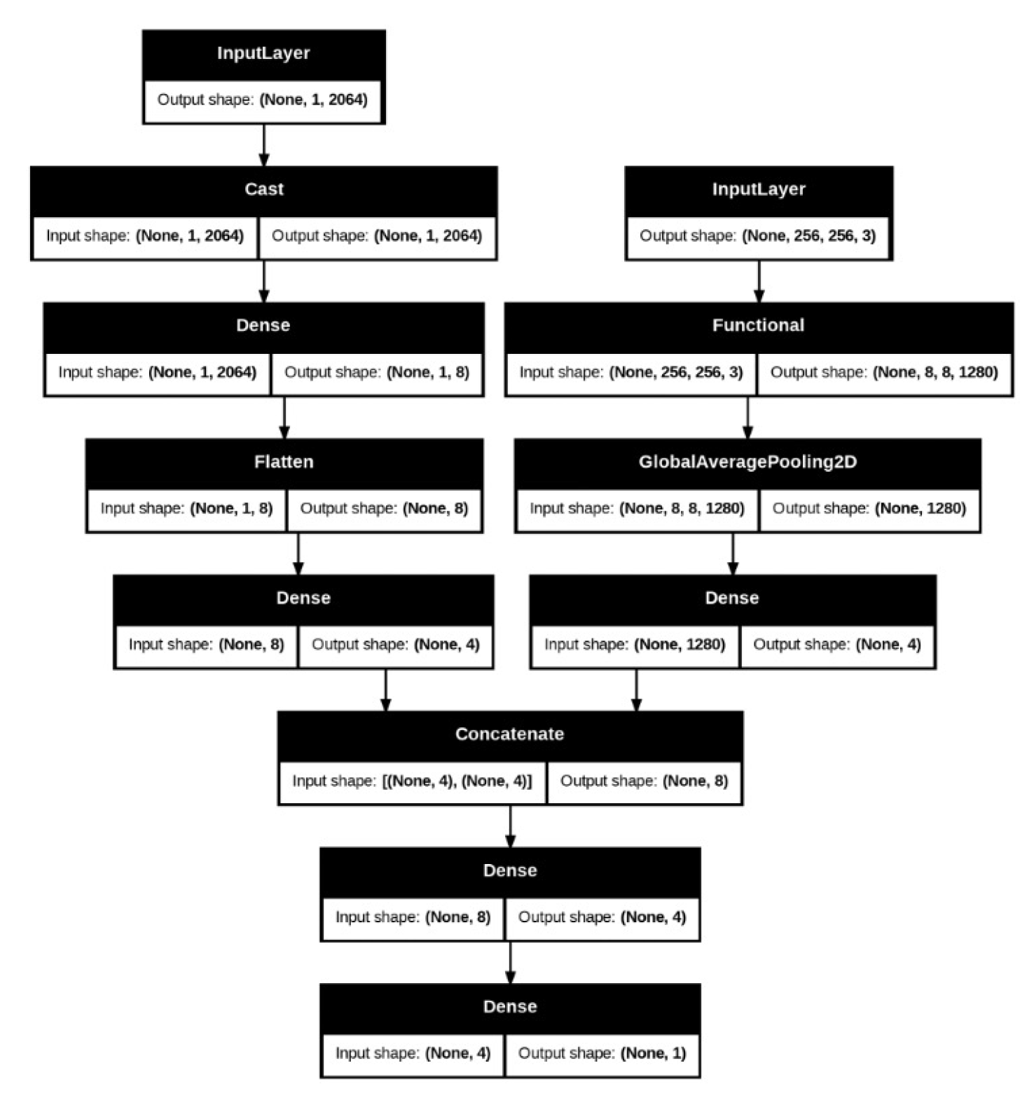
Figure 6.
Performance metrics for the CNN’s VGG16 Model Trained on Dataset 1 and tested on the other five Datasets.
Figure 6.
Performance metrics for the CNN’s VGG16 Model Trained on Dataset 1 and tested on the other five Datasets.
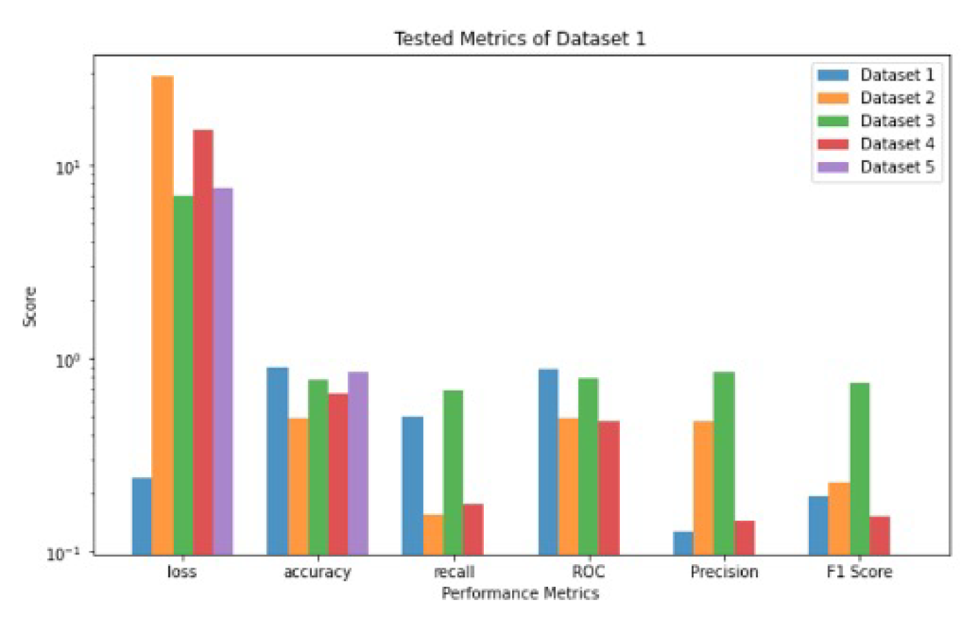
Figure 7.
Performance metrics for the CNN’s VGG16 Model Trained on Dataset 2 and tested on the other five Datasets [1,2,3,4,5].
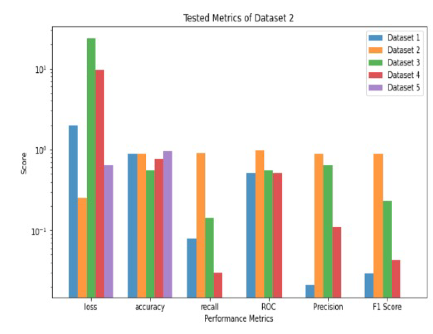
Figure 8.
Performance metrics for the CNN’s VGG16 Model Trained on Dataset 4 and tested on the other five Datasets.
Figure 8.
Performance metrics for the CNN’s VGG16 Model Trained on Dataset 4 and tested on the other five Datasets.
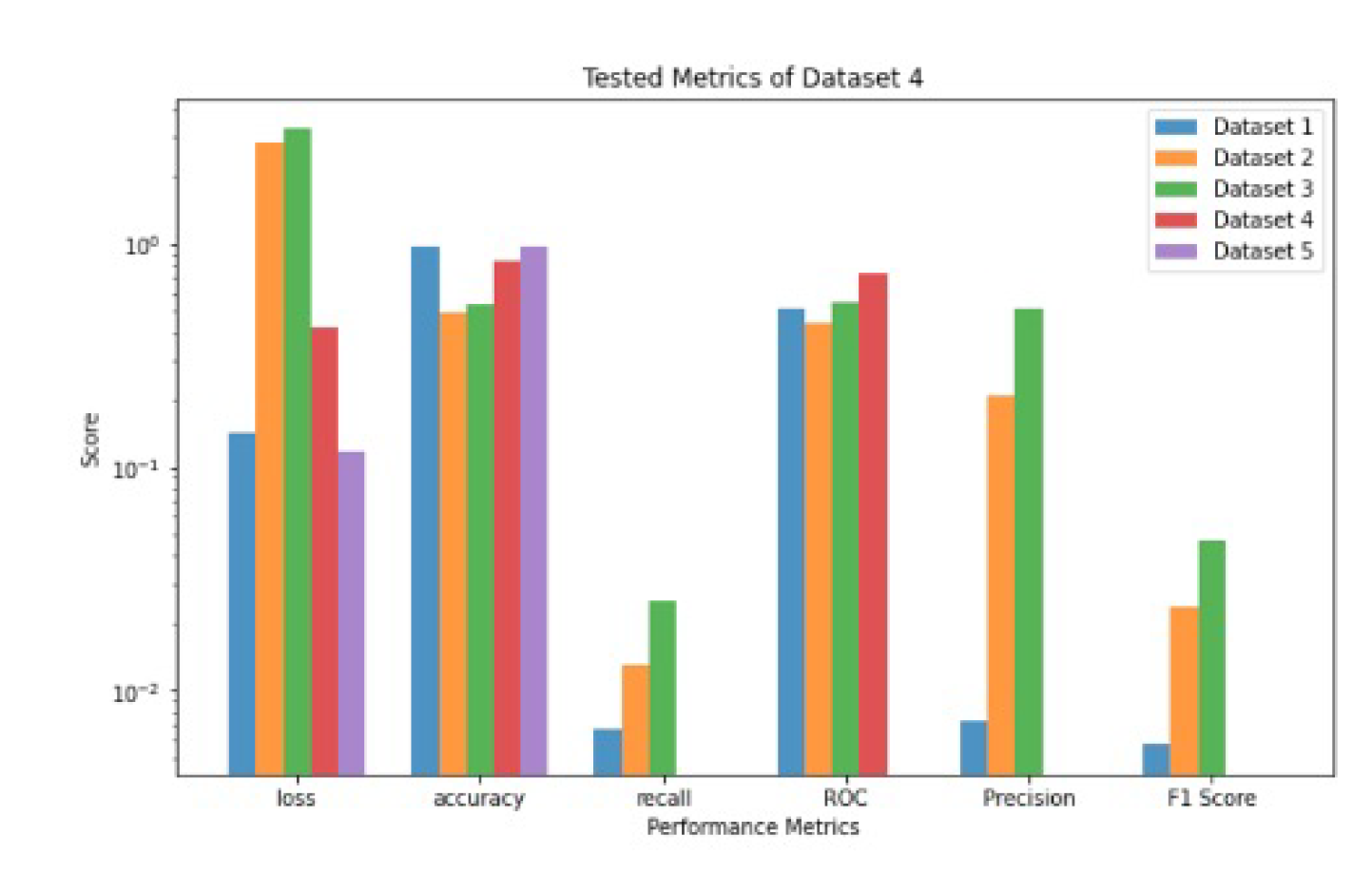
Figure 9.
Performance metrics for the CNN’s VGG16 Model Trained on Dataset 3 and tested on the other five Datasets [1,2,3,4,5].
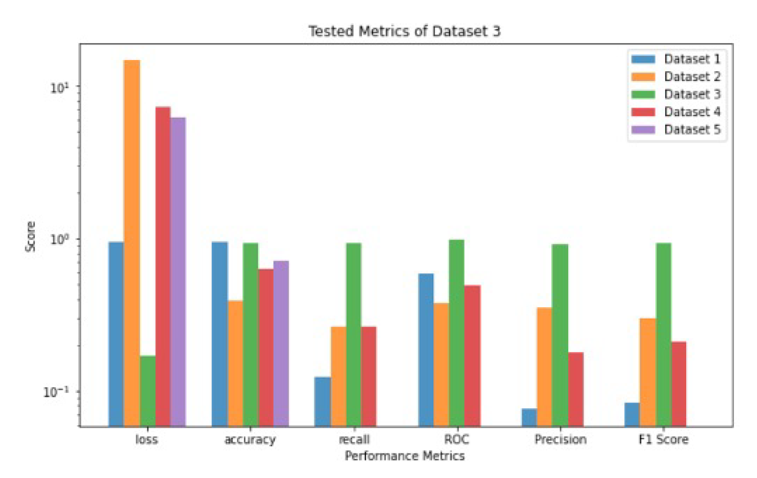
Figure 10.
Performance metrics for the CNN’s VGG16 Model Trained on Dataset 5 and tested on the other five Datasets [1,2,3,4,5].
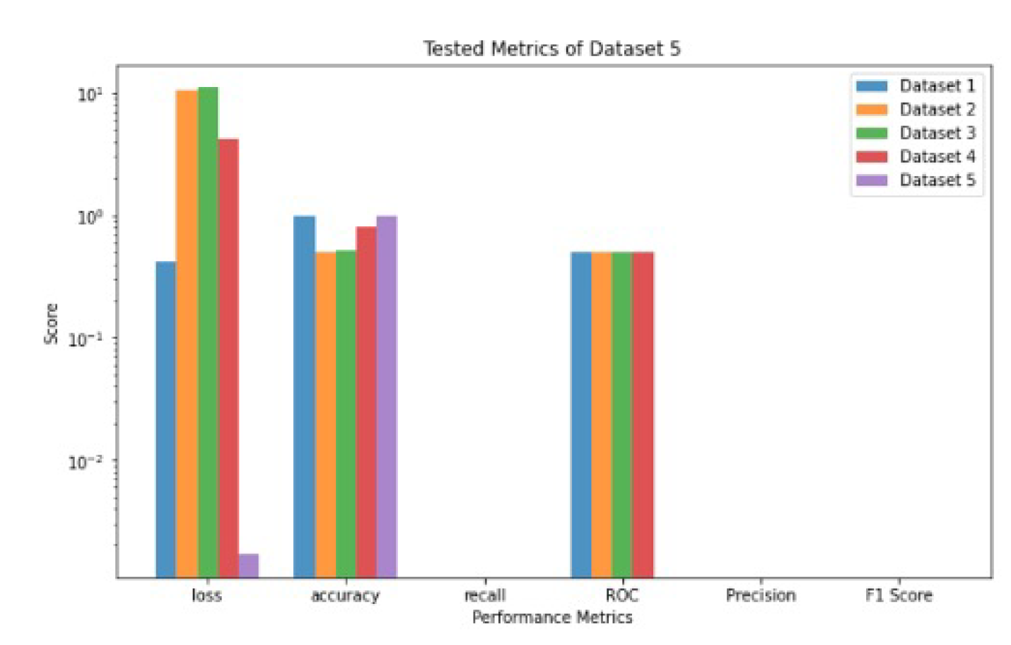
Figure 11.
Performance metrics values for Dataset 1 and trained on females only and tested on the other five Datasets [1,2,3,4,5].
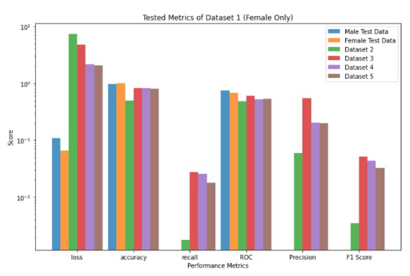
Figure 12.
Performance metrics values for Dataset 1 and trained on males only and tested on the other five Datasets [1,2,3,4,5].
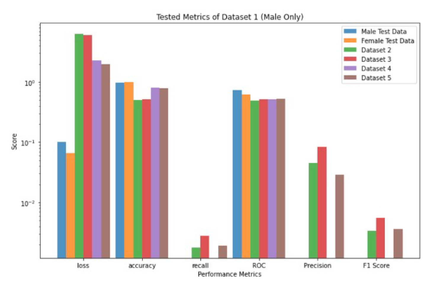
Figure 13.
Performance comparison between VGG16 and the Ensemble Model: (a) performance metrics. (b) trainable parameters.
Figure 13.
Performance comparison between VGG16 and the Ensemble Model: (a) performance metrics. (b) trainable parameters.
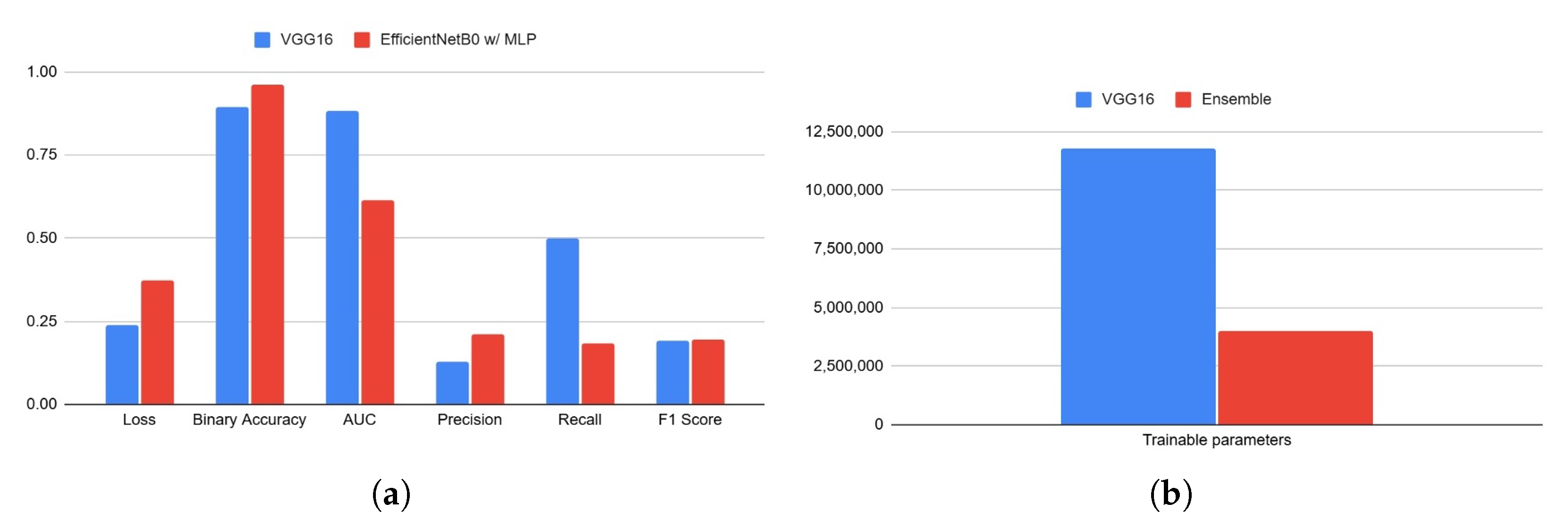
Table 1.
The split of datasets for training, testing, and validation.
| Datasets | Training (75%) | Test (12.5%) | Validation (12.5%) | Total | ||||
|---|---|---|---|---|---|---|---|---|
| Malignant | Benign | Malignant | Benign | Malignant | Benign | Benign | Malignant | |
| Dataset 1 | 438 | 24406 | 73 | 4068 | 73 | 4068 | 32542 | 584 |
| Dataset 2 | 4005 | 4005 | 668 | 668 | 668 | 668 | 5341 | 5341 |
| Dataset 3 | 3750 | 3453 | 625 | 576 | 625 | 576 | 5000 | 4605 |
| Dataset 4 | 1218 | 280 | 204 | 47 | 204 | 47 | 1626 | 374 |
| Dataset 5 | 220 | 901 | 109 | 450 | 109 | 450 | 1801 | 438 |
Table 2.
The performance metrics of CNN’s VGG16 use a sigmoidal activation function, trained on Dataset 1 and tested on the other five datasets [1,2,3,4,5].
| Metrics Datasets |
Loss | Accuracy | Recall | ROC | Precision | F1 Score |
|---|---|---|---|---|---|---|
| Dataset 1 | 0.2407 | 0.8958 | 0.501 | 0.8835 | 0.127 | 0.1926 |
| Dataset 2 | 28.7647 | 0.4903 | 0.1558 | 0.4932 | 0.4728 | 0.2294 |
| Dataset 3 | 7.0176 | 0.779 | 0.6786 | 0.7904 | 0.8532 | 0.7535 |
| Dataset 4 | 15.3016 | 0.66 | 0.1749 | 0.4702 | 0.1444 | 0.1521 |
| Dataset 5 | 7.6494 | 0.8487 | 0 | 0 | 0 | 0 |
Table 3.
The performance metrics of CNN’s VGG16 use a sigmoidal activation function, trained on Dataset 2 and tested on the other five datasets [1,2,3,4,5].
| Datasets Metrics |
Loss | Accuracy | Recall | ROC | Precision | F1 Score |
|---|---|---|---|---|---|---|
| Dataset 1 | 1.9952 | 0.8828 | 0.0782 | 0.5073 | 0.021 | 0.0293 |
| Dataset 2 | 0.2522 | 0.8852 | 0.8974 | 0.9617 | 0.8779 | 0.8859 |
| Dataset 3 | 23.521 | 0.551 | 0.1433 | 0.546 | 0.6417 | 0.2301 |
| Dataset 4 | 9.7817 | 0.7717 | 0.0296 | 0.5116 | 0.1101 | 0.0431 |
| Dataset 5 | 0.6277 | 0.9553 | 0 | 0 | 0 | 0 |
Table 4.
The performance metrics of CNN’s VGG16 use a sigmoidal activation function, trained on Dataset 4 and tested on the other five datasets [1,2,3,4,5].
| Datasets Metrics |
Loss | Accuracy | Recall | ROC | Precision | F1 Score |
|---|---|---|---|---|---|---|
| Dataset 1 | 0.1432 | 0.9776 | 0.0068 | 0.5132 | 0.0074 | 0.0058 |
| Dataset 2 | 2.7951 | 0.4914 | 0.013 | 0.4382 | 0.2089 | 0.0239 |
| Dataset 3 | 3.2474 | 0.5301 | 0.0251 | 0.5436 | 0.5072 | 0.047 |
| Dataset 4 | 0.4208 | 0.8326 | 0 | 0.7316 | 0 | 0 |
| Dataset 5 | 0.1167 | 0.981 | 0 | 0 | 0 | 0 |
Table 5.
The performance metrics of CNN’s VGG16 use a sigmoidal activation function, trained on Dataset 3 and tested on the other five datasets [1,2,3,4,5].
| Datasets Metrics |
Loss | Accuracy | Recall | ROC | Precision | F1 Score |
|---|---|---|---|---|---|---|
| Dataset 1 | 0.9409 | 0.9477 | 0.1228 | 0.5913 | 0.0764 | 0.083 |
| Dataset 2 | 14.6906 | 0.3884 | 0.2633 | 0.3746 | 0.3538 | 0.2977 |
| Dataset 3 | 0.1711 | 0.9288 | 0.9303 | 0.9821 | 0.9212 | 0.9252 |
| Dataset 4 | 7.285 | 0.6283 | 0.2661 | 0.4922 | 0.1797 | 0.2105 |
| Dataset 5 | 6.1814 | 0.7188 | 0 | 0 | 0 | 0 |
Table 6.
The performance metrics of CNN’s VGG16 use a sigmoidal activation function, trained on Dataset 5 and tested on the other five datasets [1,2,3,4,5].
| Datasets Metrics |
Loss | Accuracy | Recall | ROC | Precision | F1 Score |
|---|---|---|---|---|---|---|
| Dataset 1 | 0.4198 | 0.9824 | 0 | 0.5 | 0 | 0 |
| Dataset 2 | 10.5211 | 0.5 | 0 | 0.5 | 0 | 0 |
| Dataset 3 | 11.0315 | 0.5206 | 0 | 0.5 | 0 | 0 |
| Dataset 4 | 4.2657 | 0.805 | 0 | 0.5 | 0 | 0 |
| Dataset 5 | 0.0017 | 1 | 0 | 0 | 0 | 0 |
Table 7.
The performance metrics values for females only for dataset-1.
| Datasets Metrics |
Loss | Accuracy | Recall | ROC | Precision | F1 Score |
|---|---|---|---|---|---|---|
| MaleTestData | 0.1077 | 0.9745 | 0 | 0.7539 | 0 | 0 |
| FemaleTestData | 0.0659 | 0.9873 | 0 | 0.6763 | 0 | 0 |
| Dataset 2 | 7.3955 | 0.4979 | 0.0018 | 0.4846 | 0.0599 | 0.0035 |
| Dataset 3 | 4.7162 | 0.817 | 0.0275 | 0.5931 | 0.5408 | 0.0519 |
| Dataset 4 | 2.1413 | 0.817 | 0.0254 | 0.5247 | 0.2031 | 0.044 |
| Dataset 5 | 2.0699 | 0.8002 | 0.0181 | 0.5331 | 0.2 | 0.033 |
Table 8.
The performance metrics values for males only for dataset-1 [1].
Table 8.
The performance metrics values for males only for dataset-1 [1].
| Datasets Metrics |
Loss | Accuracy | Recall | ROC | Precision | F1 Score |
|---|---|---|---|---|---|---|
| MaleTestData | 0.1006 | 0.9769 | 0 | 0.7435 | 0 | 0 |
| FemaleTestData | 0.0658 | 0.9884 | 0 | 0.6218 | 0 | 0 |
| Dataset 2 | 6.3705 | 0.4989 | 0.0018 | 0.4932 | 0.0449 | 0.0034 |
| Dataset 3 | 6.0307 | 0.5202 | 0.0028 | 0.5156 | 0.0828 | 0.0055 |
| Dataset 4 | 2.2841 | 0.812 | 0 | 0.5209 | 0 | 0 |
| Dataset 5 | 1.9608 | 0.7979 | 0.0019 | 0.5261 | 0.0286 | 0.0036 |
Disclaimer/Publisher’s Note: The statements, opinions and data contained in all publications are solely those of the individual author(s) and contributor(s) and not of MDPI and/or the editor(s). MDPI and/or the editor(s) disclaim responsibility for any injury to people or property resulting from any ideas, methods, instructions or products referred to in the content. |
© 2026 by the authors. Licensee MDPI, Basel, Switzerland. This article is an open access article distributed under the terms and conditions of the Creative Commons Attribution (CC BY) license.
Copyright: This open access article is published under a Creative Commons CC BY 4.0 license, which permit the free download, distribution, and reuse, provided that the author and preprint are cited in any reuse.