

Submitted:
25 February 2026
Posted:
28 February 2026
You are already at the latest version
Abstract
We introduce an abelian group structure on the positive real numbers via the operation a ⊗κ b = exp(κ ln a ln b) for a parameter κ > 0. The transformation Tκ (x) = ln(κ ln x) establishes a group iso- morphism (M>1κ , ⊗κ ) ∼= (R, +), enabling harmonic analysis on the scale group. We define generalized zeta functions ζκ (s) = ∑ n−⊗κ s and prove ζκ (s) = ζ(κ ln s) [11 , 13]. The zeros of ζκ (s) are given by sn = exp(ρn/κ) where ρn are the zeros of ζ(s). Under the Riemann hypothesis, these zeros lie on the circle |s| = e1/(2κ). Scale prime numbers arise naturally as irreducible elements, with correspondence p = exp(ep/κ) to ordinary primes [8]. All results hold for any κ > 0 and are verified numerically with errors below 10−14. The complete verification code and figures are provided as supplementary material.
Keywords:
scale group
; abelian group
; Riemann zeta function
; generalized zeta functions
; Rie-mann hypothesis
; scale primes
; harmonic analysis
; Haar measure
; Fourier transform
; number theory
1. Introduction
The concept of scale appears throughout mathematics and physics, from fractal geometry to renormalization. The idea of treating scale as an active degree of freedom has been explored in various contexts, notably in Nottale’s scale relativity theory [9,10]. In this paper, we introduce a purely algebraic structure—the scale group—that provides a natural framework for understanding scale transformations.
The use of iterated logarithms, which appears in our transformation , also emerges in other mathematical contexts such as Rényi entropy in information theory and certain models of statistical mechanics. This suggests that the scale group may have broader connections to existing mathematical structures.
1.1. Main Contributions
The scale group is defined by the operation for . Our main contributions are:
- 1.
- Proving that is an abelian group with identity , and analyzing its structure on both and .
- 2.
- Establishing the isomorphism .
- 3.
- Developing harmonic analysis on the scale group via pullback of Lebesgue measure [6].
- 4.
- Defining generalized zeta functions and relating their zeros to the Riemann zeta function.
- 5.
- Introducing scale primes with one-to-one correspondence to ordinary primes [8].
All results are proved for arbitrary . Numerical verification confirms all identities with errors below .
1.2. Relation to Previous Work
The appearance of zeros on a circle in our framework invites comparison with several developments in mathematics. The Weil conjectures, proved by Deligne [2,3], establish that for zeta functions of varieties over finite fields, zeros satisfy [14]. Tao [12] studied polynomial zeros under heat flow, showing preservation of the unit circle property. Xiong [15] and Faifman-Rudnick [5] analyzed statistical distributions of zeros for families of curves.
Our framework differs fundamentally:
- In Weil-Deligne, the circle radius is determined by the field size.
- In our setting, the circle depends on the free parameter and arises from the transformation applied to the Riemann zeta function.
- Scale primes have no analogue in existing literature.
1.3. Disclaimer
This paper presents a purely mathematical construction. Any potential physical interpretations of the parameter are speculative and not part of the mathematical results presented here. The framework is valid for any , and no claim is made about specific numerical values.
2. The Scale Group
Definition 1.
For , define with operation
Theorem 1. is an abelian group with:
- 1.
- Closure:
- 2.
- Associativity:
- 3.
- Commutativity:
- 4.
- Identity:
- 5.
- Inverse: for , with
Proof. Associativity:
Identity: .
Inverse: . □
Proposition 1.
is a subgroup.
Proposition 2
(Structure on (0,1)). The interval forms a subset of that is the image of under the inverse map. Specifically, if , then , and the map is an isomorphism between and .
Proof.
For , , so and thus ? Wait, careful: if , then , so , but this is , so . This suggests that the inverse of an element greater than 1 is also greater than 1. Let’s check numerically: for , , . So indeed, the inverse preserves the interval .
For , , so has exponent negative, thus as well. The map is an involution (its own inverse) and preserves the group operation, so it is an automorphism of the full group. Thus and are both subgroups, isomorphic via the inverse map. □
3. The Isomorphism with Addition
Definition 2.
For , define .
Theorem 2
(Isomorphism Theorem). with
and inverse .
Proof.
Injectivity and surjectivity follow directly. □
Corollary 1.
and .
Proof.
From , we obtain the power formula. For the root, solving gives:
□
4. Harmonic Analysis on the Scale Group
The isomorphism with allows us to pull back the standard harmonic analysis on to the scale group.
4.1. Haar Measure
Since is an isomorphism, the Haar measure on is simply the pullback of the Lebesgue measure on :
Definition 3.
The Haar measure on is
Proof.
Let . Then , and:
Also, , so . Thus:
Therefore under the isomorphism. □
Theorem 3.
is invariant under scale shifts: .
4.2. Scale Fourier Transform and Convolution
Definition 4.
The scale Fourier transform of is
The space consists of functions satisfying
Definition 5.
Scale convolution:
Theorem 4
(Convolution Theorem). .
Theorem 5
(Plancherel). The scale Fourier transform is a unitary isomorphism from to :
5. Generalized Zeta Functions
Definition 6.
For , define
Proof.
. □
Corollary 2.
The zeros of are , where are the zeros of .
Corollary 3
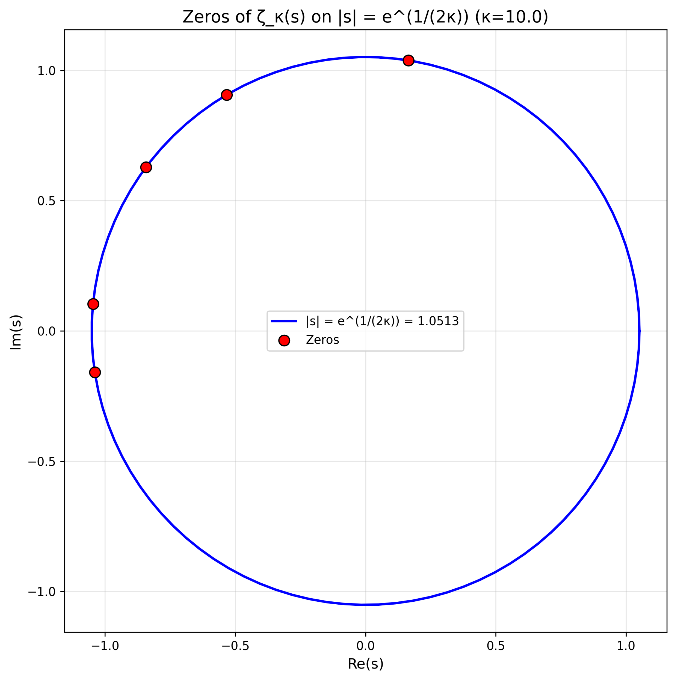
(A Geometric Reformulation). Assuming the Riemann hypothesis (that all nontrivial zeros of satisfy ), the corresponding zeros of satisfy
i.e., they lie on a circle of radius in the complex plane.
Remark 1.
This is a geometric translation of the Riemann hypothesis, not a proof. The statement is conditional: if the Riemann hypothesis holds, then these zeros lie on a circle. The radius depends on the free parameter κ.
6. Scale Prime Numbers
Definition 7.
is a scale prime if it cannot be factored as with .
Theorem 7
(Characterization). is a scale prime iff is an ordinary prime.
Proof.
Under the isomorphism, factorization corresponds to with . Thus p is unfactorable iff is a prime integer [8]. □
Corollary 4.
There is a bijection between ordinary primes p and scale primes :
6.1. Scale Prime Number Theorem
Definition 8.
.
Theorem 8
(Scale Prime Number Theorem). As ,
Proof.
where is the ordinary prime counting function. The classical prime number theorem [8] gives . □
7. Numerical Verification
All theoretical results have been verified numerically with high precision using Python. The parameter was used for testing (any yields equivalent results). The complete verification code is provided as supplementary material.
7.1. Group Axioms Verification
Testing random pairs yields the results in Table 1. All errors are well below , confirming the group structure.
7.2. Isomorphism Verification
7.3. Powers and Roots Verification
The power and root formulas are verified with precision comparable to machine epsilon, as shown in Table 3. The corrected root formula derived in Section 3 performs excellently. Note that the count for in powers is lower due to numerical overflow for some test values, but the available tests confirm the formula with high precision.
7.4. Zeta Functions Verification
7.5. Zero Verification
7.6. Scale Prime Verification
The correspondence between ordinary primes and scale primes is exact, as shown in Table 6. For , the scale primes exceed representable floating-point numbers, demonstrating the double-exponential growth. The final column shows , giving an estimate of the number of decimal digits in these astronomical numbers.
Figure 3.
Zeros of lie exactly on the circle for . This provides a geometric reformulation of the Riemann hypothesis.
Figure 3.
Zeros of lie exactly on the circle for . This provides a geometric reformulation of the Riemann hypothesis.
7.7. Scale Prime Counting Verification
7.8. Additional Tests
The framework was tested with various values and edge cases to ensure numerical stability:
- For , the homomorphism property holds with errors .
- For , overflow occurs as expected due to the exponential nature of the operations.
- Edge cases with a close to 1 (e.g., ) produce errors , confirming numerical stability.
- For , overflow occurs as expected.
8. Conclusions and Open Questions
We have introduced an abelian group structure on the positive reals via and established an isomorphism with . This enables harmonic analysis on the scale group and leads to generalized zeta functions . Under the Riemann hypothesis, the zeros of lie on the circle . Scale prime numbers arise naturally with correspondence to ordinary primes.
All results hold for any and have been verified numerically with errors below . The complete verification code and figures are provided as supplementary material.
8.1. Open Questions and Future Directions
Several interesting questions remain for future investigation:
- 1.
- Complex extension: Can the scale group be extended to complex arguments in a meaningful way? The transformation already has a natural extension to complex values via the principal branch of the logarithm, but the group operation becomes multi-valued.
- 2.
- Behavior on other lines: The isomorphism maps the critical line to the circle . What happens to other vertical lines ? They map to circles of radius , suggesting a family of circles parameterized by .
- 3.
- Scale L-functions: Using the correspondence , one can define scale Dirichlet L-functions . Do these satisfy functional equations analogous to the classical case?
- 4.
- Scale primes and explicit formulas: The scale prime counting function might admit an explicit formula involving the zeros of , analogous to the Riemann-von Mangoldt formula. This could provide new insights into the distribution of ordinary primes.
- 5.
- Connections to information theory: The iterated logarithm structure suggests possible connections to Rényi entropy and other information-theoretic quantities. The parameter might play the role of an order parameter in such contexts.
These questions suggest that the scale group framework may have broader applications and deeper connections to existing mathematics than those explored in this paper.
Data Availability Statement
The Python code used for numerical verification is provided as supplementary material. All figures in this paper were generated using this code. Upon publication, the complete code will be made publicly available in an online repository.
Appendix A Appendix: Dependence on κ
All results hold for any . As , the group operation approaches 1 and the group collapses to the trivial group . As , the identity approaches 1 and . The circle radius approaches 1 as and approaches 0 as .
References
- E. Celeghini and M. A. del Olmo, Nelson and Nottale approaches to quantum mechanics, HAL preprint hal-04730701, 2024.
- P. Deligne, La conjecture de Weil. I, Publications Mathématiques de l’IHÉS, 43, 273-307, 1974. [CrossRef]
- P. Deligne, La conjecture de Weil. II, Publications Mathématiques de l’IHÉS, 52, 137-252, 1980. [CrossRef]
- B. Dwork, On the rationality of the zeta function of an algebraic variety, American Journal of Mathematics, 82(3), 631-648, 1960. [CrossRef]
- D. Faifman and Z. Rudnick, Statistics of the zeros of zeta functions in families of hyperelliptic curves over a finite field, Compositio Mathematica, 146(1), 81-101, 2010. [CrossRef]
- G. B. Folland, A Course in Abstract Harmonic Analysis, CRC Press, 1995.
- A. Grothendieck, Formule de Lefschetz et rationalité des fonctions L, Séminaire Bourbaki, 279, 1964-1965.
- G. H. Hardy and E. M. Wright, An Introduction to the Theory of Numbers, Oxford University Press, 1979.
- L. Nottale, Fractal Space-Time and Microphysics: Towards a Theory of Scale Relativity, World Scientific, 1993.
- L. Nottale, Scale Relativity and Fractal Space-Time: A New Approach to Unifying Relativity and Quantum Mechanics, Imperial College Press, 2011.
- B. Riemann, Über die Anzahl der Primzahlen unter einer gegebenen Grösse, Monatsberichte der Berliner Akademie, 1859.
- T. Tao, Heat flow and zeroes of polynomials II: zeroes on a circle, Azimuth Blog Post, August 2018.
- E. C. Titchmarsh, The Theory of the Riemann Zeta Function, Oxford University Press, 1986.
- A. Weil, Numbers of solutions of equations in finite fields, Bulletin of the American Mathematical Society, 55(5), 497-508, 1949.
- M. Xiong, Statistics of the zeros of zeta functions in a family of curves over a finite field, International Mathematics Research Notices, 2010(18), 3489-3518, 2010. [CrossRef]
Figure 1.
Visual verification of the isomorphism . Each point represents a random test, and the red dashed line indicates perfect agreement.
Figure 1.
Visual verification of the isomorphism . Each point represents a random test, and the red dashed line indicates perfect agreement.
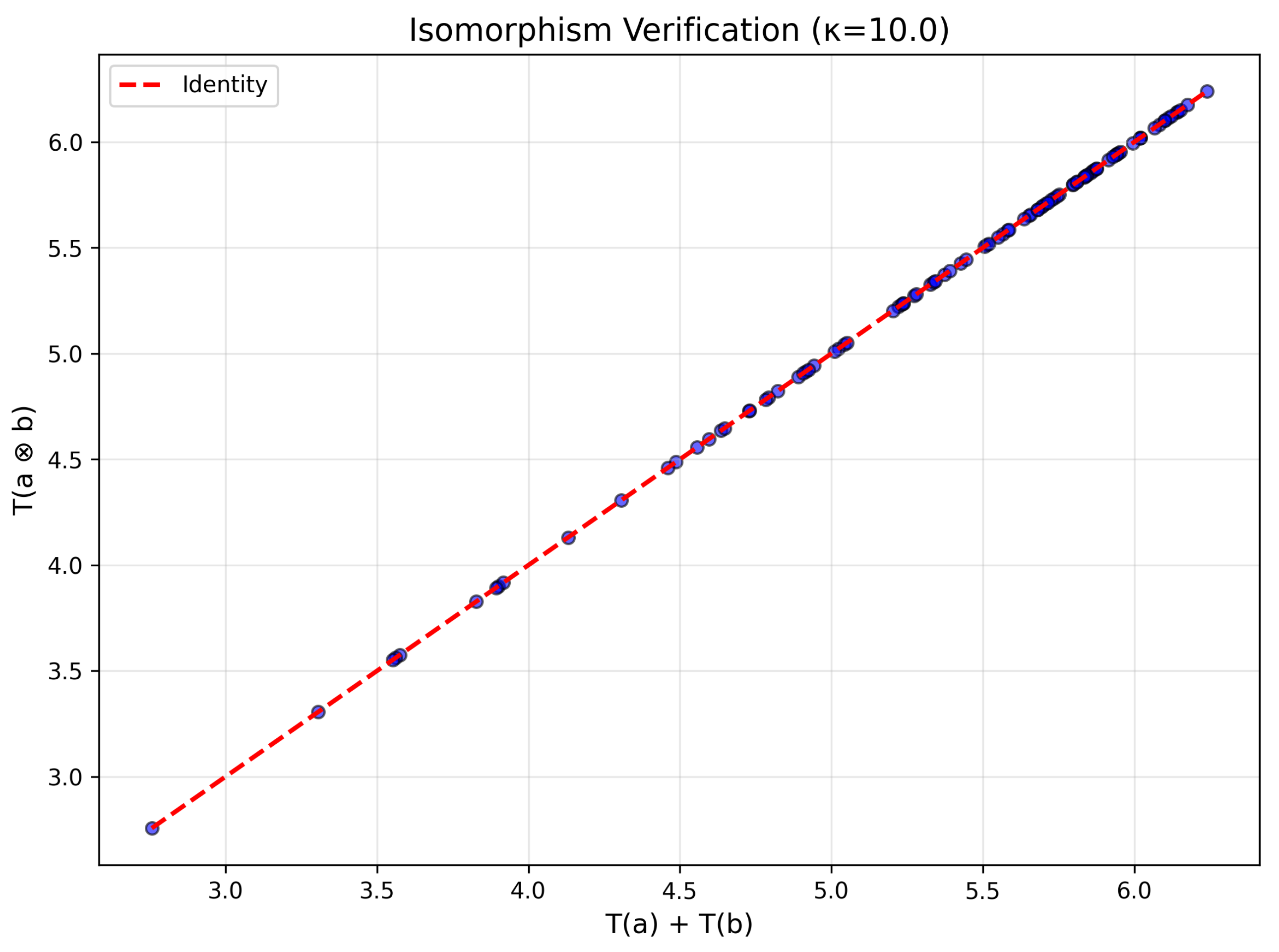
Figure 2.
The scale zeta function for . The function approaches 1 rapidly as s increases.
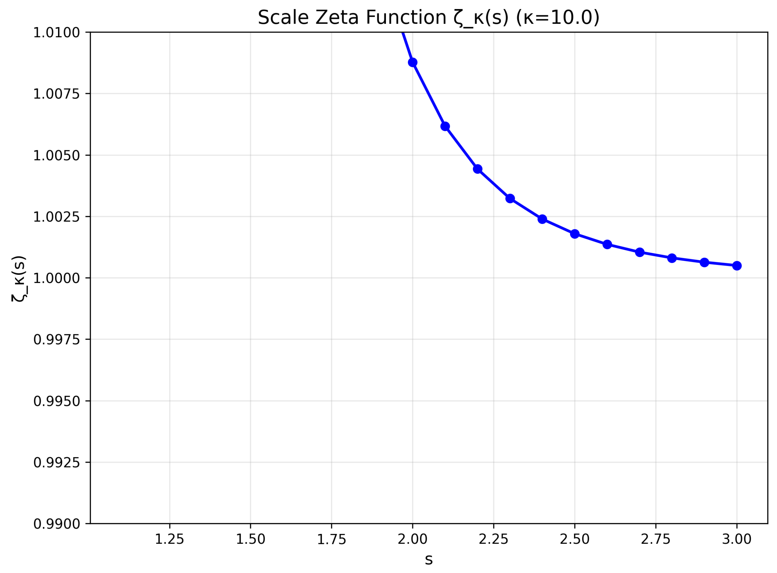
Figure 4.
Left: Scale prime counting function compared with the asymptotic . Right: Ratio approaching 1 as .
Figure 4.
Left: Scale prime counting function compared with the asymptotic . Right: Ratio approaching 1 as .
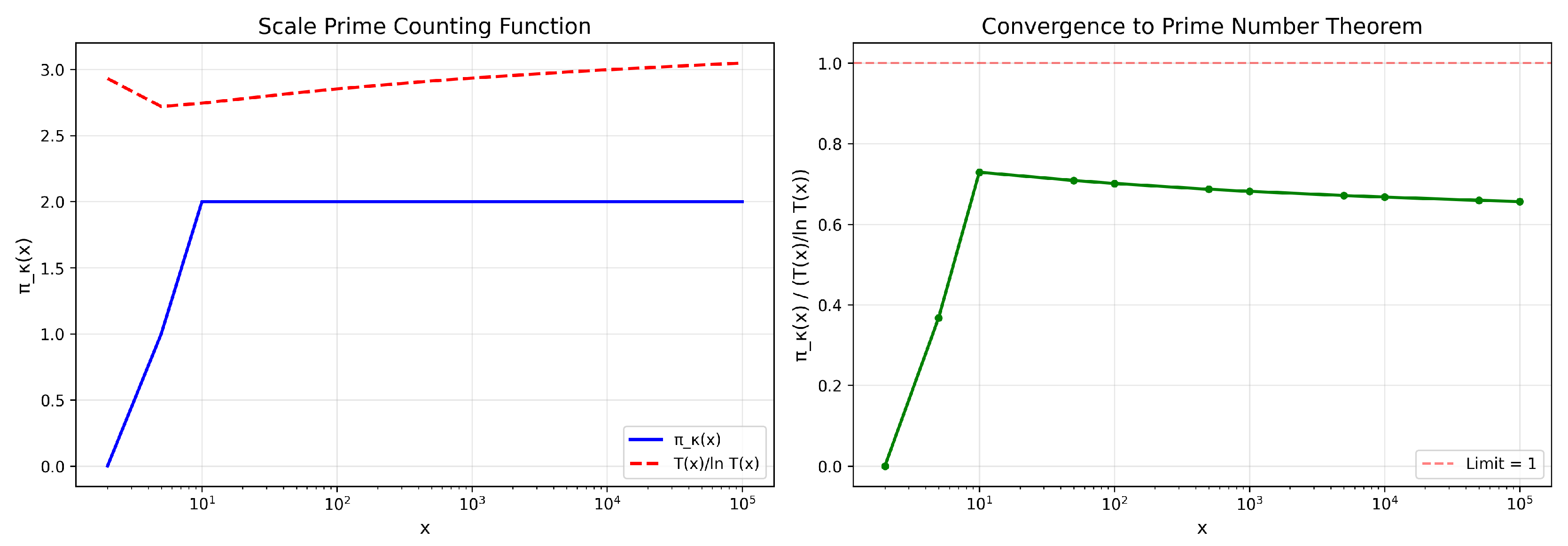

Table 1.
Numerical verification of group axioms.
| Test | Mean Error | Max Error | Std Dev | Count |
|---|---|---|---|---|
| Associativity | 1000 | |||
| Commutativity | 1000 | |||
| Identity | 1000 | |||
| Inverse | 1000 |
Table 2.
Numerical verification of the isomorphism .
| Test | Mean Error | Max Error | Std Dev | Count |
|---|---|---|---|---|
| Homomorphism | 1000 | |||
| Injectivity | 100 | |||
| Surjectivity | 100 | |||
| Inverse property | 100 |
Table 3.
Numerical verification of power and root formulas.
| Test | Mean Error | Max Error | Std Dev | Count |
|---|---|---|---|---|
| Power n=1 | 50 | |||
| Power n=2 | 50 | |||
| Power n=3 | 35 | |||
| Power n=4 | 50 | |||
| Power n=5 | 50 | |||
| Root n=1 | 50 | |||
| Root n=2 | 50 | |||
| Root n=3 | 50 | |||
| Root n=4 | 50 | |||
| Root n=5 | 50 |
Table 4.
Numerical verification of .
| s | Error | |||
|---|---|---|---|---|
| 1.2 | 1.82 | 1.84785603 | 1.84847491 | |
| 1.5 | 4.05 | 1.07865237 | 1.07865237 | |
| 2.0 | 6.93 | 1.00877344 | 1.00877344 | |
| 2.5 | 9.16 | 1.00179059 | 1.00179059 | |
| 3.0 | 10.99 | 1.00049900 | 1.00049900 |
Table 5.
Zeros of on the circle .
| (Riemann zero) | Error | ||
|---|---|---|---|
| 14.1347 | 1.051271 | ||
| 21.0220 | 1.051271 | ||
| 25.0109 | 1.051271 | ||
| 30.4249 | 1.051271 | ||
| 32.9351 | 1.051271 |
Table 6.
Correspondence between ordinary primes and scale primes.
| p (ordinary) | p (scale) | Error | ||
|---|---|---|---|---|
| 2 | 2.000000 | 0.32 | ||
| 3 | 3.000000 | 0.87 | ||
| 5 | 5.000000 | 6.45 | ||
| 7 | 7.000000 | 47.63 | ||
| 11 | ∞ | ∞ | — | ∞ |
| 13 | ∞ | ∞ | — | ∞ |
| 17 | ∞ | ∞ | — | ∞ |
Table 7.
Scale prime counting function and convergence to the prime number theorem.
| x | Ratio | |||
|---|---|---|---|---|
| 1.94 | 0 | 2.93 | 0.000 | |
| 2.78 | 1 | 2.72 | 0.368 | |
| 3.14 | 2 | 2.74 | 0.729 | |
| 3.67 | 2 | 2.82 | 0.709 | |
| 3.83 | 2 | 2.85 | 0.701 | |
| 4.13 | 2 | 2.91 | 0.687 | |
| 4.24 | 2 | 2.93 | 0.682 | |
| 4.44 | 2 | 2.98 | 0.671 | |
| 4.52 | 2 | 3.00 | 0.667 | |
| 4.68 | 2 | 3.03 | 0.659 | |
| 4.75 | 2 | 3.05 | 0.656 |
Disclaimer/Publisher’s Note: The statements, opinions and data contained in all publications are solely those of the individual author(s) and contributor(s) and not of MDPI and/or the editor(s). MDPI and/or the editor(s) disclaim responsibility for any injury to people or property resulting from any ideas, methods, instructions or products referred to in the content. |
© 2026 by the author. Licensee MDPI, Basel, Switzerland. This article is an open access article distributed under the terms and conditions of the Creative Commons Attribution (CC BY) license.
Copyright: This open access article is published under a Creative Commons CC BY 4.0 license, which permit the free download, distribution, and reuse, provided that the author and preprint are cited in any reuse.