
Submitted:
16 February 2026
Posted:
27 February 2026
You are already at the latest version
Abstract
In healthcare organizations, ransomware threats are on the rise, resulting in a greater disruption of critical patient care operations, yet current cybersecurity approaches are mostly reactive rather than proactive. As part of this study, a systematic comparative evaluation of traditional machine learning versus deep learning methodologies on small-scale tabular cybersecurity datasets characteristic of healthcare security operations is conducted to address the critical knowledge gap regarding optimal algorithmic approaches for healthcare ransomware threat prediction. In this study, the Healthcare Ransomware Dataset is used, which contains 5,000 simulated attack records with no missing values across 16 attributes capturing organizational attributes, attack characteristics, and outcome metrics. This study evaluated eight machine learning algorithms (Logistic Regression, Decision Tree, Random Forest, Gradient Boosting, Extra Trees, AdaBoost, Naive Bayes, K-Nearest Neighbors) and eight neural network architectures (Simple Deep Neural Network, Wide Deep Neural Network, Residual DNN, CNN_1D, LSTM, GRU, Ensemble DNN) across five performance dimensions: accuracy, precision, recall, F1-score, and ROC-AUC. According to the feature importance analysis, there is a strong correlation between organizational size (27.94%), recovery time (16.18%), and data restoration (12.06%) which account for 56% of the predictive power. A gradient boosting approach achieved 84.1% accuracy with 95.19% ROC-AUC and Simple DNN represented the best deep learning architecture with 85.2% accuracy and 95.44% ROC-AUC using only 12,355 parameters. As compared to machine learning (5.19%), deep learning demonstrated significantly lower performance variance (1.64% standard deviation). Across all sequence architectures (CNN_1D, LSTM, GRU), sequential architectures consistently underperformed by 2.6-4.5 percentage points, confirming the architectural mismatch for unordered tabular features. Based on the results of the analysis, Simple DNN provides the highest predictive accuracy (85.2%) for healthcare ransomware threat assessment. The complexity of an architecture beyond shallow dense networks yields diminishing returns without improving accuracy. In comparison to traditional machine learning ap-proaches, deep learning offers superior consistency across a variety of architectures. It is recommended that Simple DNN be de-ployed as the primary prediction model and Gradient Boosting be used as the fault-tolerant backup model. It is important to place a high priority on the eight top features that capture 90 percent of the predictive power of data. In the case of unordered tabular cybersecurity data, sequential architectures (CNNs, LSTMs, GRUs) should be avoided.
Keywords:
healthcare cybersecurity
; ransomware
; machine learning
; deep learning
; tabular data
; gradient boosting
; simple DNN
; neural network architecture
I. Introduction
A cybersecurity crisis is affecting healthcare organizations worldwide. It is characterized by the systematic targeting of critical medical infrastructure through increasingly sophisticated ransomware attacks [1]. From isolated incidents, these attacks have evolved into coordinated threats that could have catastrophic consequences for patient safety and operational continuity. There are many factors that have led to the healthcare sector becoming a particularly attractive target for cybercriminals, including the storage of highly sensitive patient data, including personal health information and financial records [1,2]. Managing critical care systems that cannot tolerate operational downtime without compromising patient outcomes is critical, as well as operating legacy infrastructure that contains known vulnerabilities that persist as a result of the challenges associated with patching medical devices and maintaining regulatory compliance during system updates [3]. A combination of these vulnerabilities creates an operational environment that is highly susceptible to ransomware attacks in which the consequences of successful breaches extend beyond financial losses to include immediate threats to human health and safety [3]. In contrast to other industries facing similar cybersecurity threats, the healthcare sector has a number of unique operational characteristics that create particular vulnerabilities. For informed clinical decision-making, patient care requires immediate and continuous access to comprehensive medical records, and accurate historical data is critical to avoiding adverse drug interactions and ensuring appropriate therapeutic interventions [4]. Diagnostic equipment relies upon interconnected networks that integrate imaging systems, laboratory information systems, and electronic health records into cohesive care coordination platforms. When ransomware encryption renders these systems inaccessible, healthcare providers face untenable choices between paying substantial ransoms to criminal enterprises or accepting significant delays in the delivery of care, which may result in patient harm, adverse outcomes, or even mortality in critical care situations [5]. Health care ransomware incidents differ fundamentally from similar attacks targeting commercial enterprises in that they are driven by distinctive operational pressures, in combination with ethical imperatives that prioritize patient welfare over financial considerations. However, operational disruptions, although costly, rarely have direct impacts on human survival or well-being [6].
Healthcare organizations have been consistently identified as the sector experiencing the highest per-record breach costs in IBM's annual Cost of a Data Breach Report, which documents the escalating severity and frequency of ransomware attacks. In addition to regulatory penalties and litigation expenses, protected health information has a specialized nature and typically exceeds general industry averages by significant margins [7]. Despite increased security investments, Sophos' State of Ransomware in Healthcare report further demonstrates that attack frequency continues to increase year-over-year. Therefore, traditional reactive security measures, such as perimeter defenses, signature-based malware detection, and post-incident response protocols, are systematically insufficient to address the evolving threat landscape [8]. A comprehensive industry analysis indicates that healthcare organizations require a fundamentally different approach to cybersecurity, which emphasizes predictive threat assessment and proactive vulnerability remediation, as opposed to reactive incident response. Successful attacks have operational consequences that far exceed the costs associated with preventive security investments, as patient care disruptions, regulatory investigations, and reputational damage are among the operational consequences of successful attacks [9].
The underlying patterns of attacker behavior, organizational vulnerabilities, and incident outcomes of ransomware threats have been revealed by a detailed examination of the ransomware threat landscape, suggesting the feasibility of computational modeling approaches for predicting attack likelihoods and potential impacts before breaches occur [10]. According to empirical data, adversaries consistently target healthcare organizations exhibiting particular size profiles, with medium-sized organizations experiencing the greatest frequency of attacks due to the intersection of sufficient financial resources to pay ransoms and inadequate cybersecurity infrastructure investment as compared to large healthcare systems. As a general rule, attack vectors follow predictable distributions, with compromised credentials, exploited software vulnerabilities, and phishing campaigns making up the overwhelming majority of initial breach mechanisms [10,11]. Attack outcomes are correlated with organizational preparedness metrics such as backup infrastructure quality, incident response plan maturity, and security monitoring capabilities, including recovery time duration, data restoration success rates, and operational disruption severity. In light of these observable patterns in the attack lifecycle from initial compromise through lateral movement, encryption, and recovery, machine learning algorithms and deep learning algorithms may be able to identify at-risk organizations proactively by analyzing organizational characteristics, historical incident patterns, and technical infrastructure attributes in order to generate predictive risk assessments [12].
There is a predominant tendency for healthcare organizations to adopt a reactive approach to cybersecurity. Consequently, incident response protocols have been initiated only after successful breaches have been detected, vulnerability management programs prioritize patching based on observed exploits instead of predictive risk modeling, and security investment decisions are influenced by compliance requirements and post-incidence lessons learned rather than forward-looking threat intelligence [12]. When security teams detect and respond to active encryption activities, critical systems have already been compromised, patient care delivery has been disrupted, and the organization has to decide between paying ransom or trying to restore it [12. 13]. This reactive paradigm systematically fails to prevent catastrophic operational disruptions caused by ransomware attacks. Organizations in the healthcare sector require a fundamental shift in paradigm toward the capability of assessing threats in a predictive manner [13]. The system should enable security teams to identify and remediate vulnerabilities before adversaries exploit them, prioritize security investments based on quantified risk rather than compliance checklists, and allocate defensive resources to protect the organizational assets and configurations which empirical data indicates correlate most strongly with successful attack prevention and rapid recovery [13].
Pattern recognition using machine learning methodologies is a powerful computational method of analyzing complex, high-dimensional datasets that are characterized by non-linear relationships among features. Thus, these techniques are ideal for cybersecurity applications where the success of an attack depends on the interaction between organizational characteristics, technical configurations, and adversarial capabilities [14]. In machine learning, traditional algorithms such as logistic regression for establishing linear baseline relationships, decision trees for capturing hierarchical decision rules that mimic human reasoning, and ensemble methods such as random forests and gradient boosting for aggregating multiple weak learners into robust predictive models have demonstrated substantial success across diverse application domains from fraud detection to medical diagnosis [14]. It is a distinct advantage of these techniques to identify non-linear relationships among input features, and to model conditional dependencies in which one variable has a significant impact on the values of another variable. Furthermore, interpretable decision rules enable domain experts to understand and validate model reasoning, which proves particularly valuable in healthcare contexts where security teams are required to provide transparent explanations for risk assessments to justify resource allocation decisions and demonstrate compliance with regulatory oversight standards [14,15].
In artificial intelligence, deep learning represents a relatively new paradigm characterized by neural network architectures with multiple hidden layers capable of automatically identifying hierarchical representations of features without requiring extensive manual feature engineering [15]. There are distinct advantages to these technologies in certain classes of problems where optimal feature transformations are not readily apparent to humans. Using convolutional neural networks, computer vision applications have been revolutionized by automatically learning spatial feature hierarchies based on raw pixel data. In natural language processing and time series prediction, recurrent architectures with long short-term memory networks have demonstrated breakthrough performance by modeling long-range temporal dependency networks [16]. A deep feedforward network has also demonstrated the capability of approximating arbitrarily complex functions when sufficient training data and an appropriate architecture are available. It should be noted, however, that to effectively constrain the immense parameter spaces that characterize multilayer neural networks, large-scale datasets containing hundreds of thousands or millions of training examples are typically required for deep learning to be applied successfully [16. 17]. There are important questions raised regarding the applicability and effectiveness of these methods in the context of healthcare cybersecurity datasets that have limited incident reporting capabilities, data sharing restrictions due to privacy regulations, and the recent emergence of systematic ransomware targeting, which collectively limit the number of records that are available for training [17].
In the cybersecurity analytics literature, the comparative evaluation of traditional machine learning approaches versus deep learning approaches for healthcare ransomware prediction addresses a critical knowledge gap. Due to the fact that most existing comparative studies focus on application domains characterized by large-scale datasets, such as computer vision tasks involving millions of labeled images, A natural language processing system that utilizes extensive text corpora, and a recommendation system that utilizes billions of user interactions [18]. However, limited empirical evidence has been provided regarding the relative performance of these paradigms with respect to the data in healthcare cybersecurity inci[19,20dent repositories that are structured tabular in nature. The lack of knowledge in this area creates substantial uncertainty for healthcare organizations and security vendors interested in developing and deploying predictive threat assessment systems [19]. Due to the lack of evidence-based guidance, decision-makers are uncertain which algorithmic approaches are most effective given realistic constraints on data availability, and whether deep learning architectures provide potential accuracy improvements over traditional methods despite their infrastructure complexity and computational overhead [19,20]. This paper describes the performance trade-offs between predictive accuracy, computational efficiency, model interpretability, and operational robustness in mission-critical healthcare security applications, and how these trade-offs should be taken into consideration when selecting algorithms [20].
In this research, the Healthcare Ransomware Dataset (2024-2025) provides a rigorous methodological basis for evaluating comparative algorithms. 5,000 carefully simulated attack records are utilized to capture the multifaceted impact of ransomware incidents across a wide range of healthcare organizations, including hospitals, outpatient clinics, insurance companies, pharmaceutical manufacturers, and research laboratories [21]. In this comprehensive dataset, each record represents a unique attack scenario that incorporates detailed variables spanning organizational attributes. Among these attributes are entity type classification, employee count-based size classification, and cybersecurity monitoring frequency; attack characteristics such as temporal occurrence patterns, identification of the initial breach vector, infection rate percentages measuring the severity of system compromises, and counts of affected facilities indicating successful lateral movements [21,22]. Additionally, historical incident frequency measures organizational exposure to repeated targeted threats as well as operational impact metrics, including recovery time duration in days, restoration success percentages, binary outcome flags indicating backup system compromises, data encryption occurrences, information exfiltration, and ransom payments [23]. Throughout the dataset construction process, empirical patterns documented in authoritative industry publications were deliberately incorporated into the simulation methodology. Using IBM's Cost of a Data Breach analysis and Sophos' healthcare ransomware research reports, synthetic attack records reflect the cybersecurity dynamics observed in actual healthcare breaches while circumventing the ethical, legal, and practical challenges associated with accessing and analyzing genuine patient-impacting data breaches [22,23].
As a result of preliminary feature im[21,22portance analysis conducted using tree-based ensemble methods, striking hierarchical contributions emerged within the dataset's predictor variables, with organizational size emerging as the overwhelmingly dominant feature accounting for 27.94% of total predictive power nearly twice as much as the second-ranked feature and significantly exceeding the combined importance of the following four features [24]. Due to the extreme dominance of organizational scale, structural characteristics fundamentally determine ransomware vulnerability and impact severity independently of specific attack vectors or security posture variations, as larger organizations have more complex interconnected systems and larger attack surfaces [25]. In addition, large organizations possess greater financial resources, which makes them more attractive ransom targets, while smaller organizations operate simpler infrastructures that may be easier to secure, but lack dedicated security personnel and sophisticated defensive measures [25]. In addition to recovery time contributing 16.18% of predictive importance, data restoration percentage contributed 12.06%, and together these three features captured 56.18 percent of the overall predictive signal. This pattern demonstrates a striking manifestation of the Pareto principle in cybersecurity prediction, where approximately 20% of input features provide greater than 50% predictive value. This concentration pattern has significant implications for operational monitoring strategies and model optimization methods [26].
This dataset has been comprehensively analyzed across five validation dimensions to determine whether it is of exceptional quality and analytically appropriate. Missing values were detected, duplicate records were identified, cardinality was analysed, consistency was verified, and validity was checked [26,27]. The analysis revealed no missing values across all 5,000 records and 16 features, no duplicate observations despite the large sample size, appropriate diversity within categorical variables reflecting realistic organizational and attack heterogeneity, and consistent encoding of data types without any format inconsistencies or typographical errors [27]. There are continuous variables with logical ranges, percentage-based metrics within [0,100] intervals, count variables with non-negative integer values, and temporal values that fall within plausible chronological boundaries for the 2024 observation period [28]. This exceptional data quality eliminates the preprocessing complexity typically required for real-world datasets characterized by missing data requiring imputation, duplicates necessitating deduplication logic, inconsistent encodings requiring normalization procedures, and validity violations requiring outlier treatment decisions, which allows researchers to focus analytical efforts on developing and evaluating substantive models rather than cleaning data [28]
II. Background
- A.
- Machine Learning and Deep Learning:
Machine Learning (ML) and Deep Learning (DL) are transformative branches of Artificial Intelligence (AI) that have significantly improved cybersecurity, particularly in detecting sophisticated threats like ransomware. In machine learning, algorithms are trained on historical data in order to recognize patterns and make decisions without explicit programming [27,28,29]. In cybersecurity, machine learning models are trained on datasets that contain both benign and malicious software samples in order to classify unknown files according to the learned features [30,31]. An example of a machine learning technique that is commonly used is Decision Trees (DT), Random Forests (RF), Support Vector Machines (SVM), and K-Nearest Neighbors (KNN). It is advantageous to use these models for the initial screening of threats since they are effective at identifying known malware signatures and behavioural anomalies [32,33].
Deep Learning, a subset of machine learning, uses multilayered neural networks, such as Convolutional Neural Networks (CNNs), Recurrent Neural Networks (RNNs), and Transformers, to automatically extract complex features from raw data [34,35]. By contrast with traditional machine learning, which often requires the creation of manual features, deep learning is capable of learning hierarchical representations directly from inputs such as file binaries, logs, or network traffic [36]. Through this capability, DL models can detect subtle and evolving patterns associated with advanced ransomware that may evade rule-based or signature-based detection systems [37]. A study conducted by Sharmeen et al. compared a variety of classifiers, including CNN, SVM, RF, and a multi-class classifier (MCC) to detect Windows ransomware by deduplicating 483 ransomware samples and 754 benign samples [38]. In their study, they found that deep learning models, in particular CNNs, were more effective at identifying encrypted payloads and obfuscated code structures when compared to traditional machine learning methods [39,40,41].
Machine Learning Paradigms in Ransomware Detection
This paper presents a review of three primary paradigms of machine learning that have proven effective in the detection of ransomware, each with a substantial body of empirical evidence supporting its effectiveness [42]. The use of supervised learning has shown remarkable success in the classification of ransomware samples as well as benign samples. It is dependent on labelled data that can be trained on. Using supervised learning algorithms including Decision Trees (DT), Random Forests (RF), K-Nearest Neighbors (K-NN), Naive Bayes (NB), and Gradient Boosting, Zhang et al. (2019) achieved 99.3% accuracy in the classification of ransomware families using Decision Trees (DT), Random Forests (RF), and K-Nearest Neighbors (K-NN) [43,44,45]. Based on opcode density alone, Baldwin and Dehghantanha (2018) demonstrate that Support Vector Machines (SVM) are particularly effective in classifying ransomware families based on 96.5% accuracy. The concept of unsupervised learning implies that the data does not need to be labelled, which has proven to be extremely useful in detecting zero-day ransomware variants [46]. By grouping similar behavioural patterns together, clustering algorithms such as k-means and fuzzy C-means have shown to be successful in identifying previously unknown ransomware families that have previously been unknown [47]. In recent years, it has been shown that dimension reduction techniques like Principal Component Analysis (PCA) and Linear Discriminant Analysis (LDA) have enhanced detection accuracy while reducing computational overhead. In some studies, it has been shown that processing speed can be improved up to 15% without sacrificing detection accuracy [48,49,50].
Deep Learning Architectures and Evidence of Effectiveness
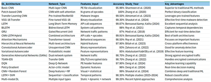
A number of studies have demonstrated that deep learning architectures are extremely effective when it comes to the detection of ransomware, providing persuasive evidence that they are superior to traditional methods. According to Sharmeen et al. (2020), a study published in the Journal of Neural Information Processing Techniques shows that Convolutional Neural Networks (CNNs) have shown remarkable success in analysing visual representations of malware, with a recent study finding 95.96% accuracy using CNN architectures for the detection of Windows ransomware (35). Compared to traditional machine learning classifiers (SVMs, Random Forests, and multi–class classifiers), CNNs outperformed SVMs (89.98%), Random Forests (90.95%), and multiclass classifiers (88.12%) significantly in the study. There has been a recent influx of interest in Long Short-Term Memory (LSTM) networks for the purpose of sequential data analysis, with Roy et al. (2021) developing DeepRan, a BiLSTM-based detector that has achieved superior performance in detecting ransomware through attention-based mechanisms that have been shown to be effective (36). The latest evidence from transfer learning studies indicates that pre-trained CNN models can achieve up to 99.5% accuracy when fine-tuned for ransomware detection, which was demonstrated by Almomani et al. (2023) by leveraging transfer-learned features from ResNet and other pre-trained architectures (37).
Static Analysis Techniques with AI Enhancement
Recent studies have shown that static analysis enhanced by artificial intelligence provides significant improvements in detection efficiency compared with traditional signature-based methods, with substantial evidence that it is effective. Poudyal and Dasgupta (2021) achieved 99.72% accuracy and 0.003 false positive rates with their tri-gram TF-IDF methods combined with Support Vector Machines, showing that n-gram analysis of opcodes is particularly successful (38). A PE header analysis enhanced with machine learning has demonstrated consistent results across multiple studies and new research has proven that header-based features combined with AI algorithms can detect packed and obfuscated ransomware with an accuracy of over 97% when combined with header-based features [39,46,49]. A study showed that using AI-enhanced entropy calculations can detect between legitimate encrypted payloads and malicious ransomware encrypted payloads with a 95% accuracy rate, and entropy analysis using machine learning models has shown to be effective for identifying encrypted payloads [40,41,48]. It has been found that string analysis combined with natural language processing techniques can be used to identify malicious strings and URLs embedded in ransomware samples with a minimal number of false positives, with studies indicating that AI models can detect malicious strings and URLs embedded in ransomware samples with minimal false positives [42,48].
Dynamic Analysis and Behavioral Detection Methods
There has been significant progress in behavioral-based ransomware detection over the last few years, enabled by dynamic analysis powered by artificial intelligence, which has a substantial body of recent research supporting its efficiency [49,50]. Using Gradient Boosted Trees for dynamic feature analysis to analyse API calls sequences, Herrera-Silva and Hernández-Alvarez (2023) achieved 99% accuracy with the use of Gradient Boosted Trees for API call sequence analysis using machine learning. In the study of Homayoun et al. (2019), it has been demonstrated that behavioural modelling through machine learning algorithms has been highly effective [44,50,51]. By employing frequent pattern mining approaches, (2019) achieved 99% accuracy in detecting ransomware instances from benign samples, and 96.5% accuracy in identifying specific ransomware families. In recent studies, LSTM networks have been demonstrated to have the capability of identifying malicious system call patterns with an accuracy of over 98% while maintaining low false positive rates in terms of system call analysis enhanced with deep learning [44,51,52]. Monitoring the file system in conjunction with machine learning has proven to be an efficient tool for real-time detection, with evidence showing that AI-enhanced file system analysis can detect ransomware encryption activities within seconds of the inception of the attack [53,54].
Ensemble Learning and Hybrid Approaches
Recent evidence indicates that ensemble learning techniques have demonstrated superior performance compared to individual algorithms for detecting ransomware, with substantial recent evidence supporting their effectiveness in detecting ransomware [55,56]. It has consistently been shown that Random Forest algorithms have shown excellent results across multiple studies, and research has indicated that they are capable of detecting ransomware in a wide range of situations up to 97% accurate [46,57]. According to a study demonstrated results of ensemble methods combining Decision Trees, SVM, Random Forest, and AdaBoost have shown significant improvements over individual classification methods [58]. Their proposed model achieved high accuracy and F1 scores while outperforming traditional methods in identifying ransomware applications by outperforming traditional methods [47,59,60]. There have been several studies showing the potential benefits of hybrid approaches, which combine static and dynamic analysis of the malware, with Hassan and Rahman. (2017) achieving remarkable accuracy by employing Hierarchical Neural Networks for cross-platform ransomware fingerprinting based on hybrid features [48,64]. It has been shown by Hasan and Rahman (2017) that hybrid approaches that combine static and dynamic analyses, including samples from recent ransomware families such as WannaCry, outperform single-method approaches when it comes to detecting ransomware accurately and defending against evasion techniques significantly [48]
Real-Time Detection and Advanced AI Techniques
It has been proven that the use of artificial intelligence for real-time ransomware detection has shown tremendous promise, with recent evidence showing significant improvements in terms of response times and accuracy of this method [49]. As reported by Mehnaz et al. (2018), RWGuard is a real-time detection mechanism that achieves zero false negatives and minimal false positives by constantly monitoring processes and file systems, an approach that achieves zero false negatives and minimal false positives [49]. In a recent study conducted by Zuhair and colleagues (2020), they devised a multi-tier streaming analytics model that outperformed competitive anti-ransomware technologies with 97% classification accuracy in the detection of zero-day ransomware attacks. Researchers have demonstrated the ability of advanced methods such as adversarial learning to improve the resilience of detection models that are vulnerable to evasion attacks by up to 25%, with studies demonstrating the efficacy of adversarial training for developing robust detection models [50]. As a result of transfer learning applications in ransomware detection, the results have been impressive, and recent research indicates that pre-trained models can provide detection accuracy comparable to or even higher than custom-trained models with significantly fewer computational resources and training time needed [51,52,53].

Table 1.
Machine Learning Techniques.
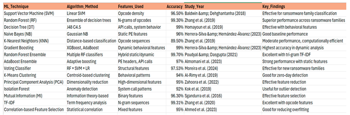 |
Table 2.
Deep Learning Techniques.
 |
Novelty and Uniqueness of the Research Area
Healthcare organizations lack effective predictive analytical tools for assessing ransomware vulnerability and forecasting likely attack outcomes based on organizational characteristics, security posture indicators, and historical incident patterns. As a result, security teams have to operate reactively, responding to breaches after operational damage has occurred rather than proactively identifying and remediating vulnerabilities [55,56,57]. Without quantified risk assessments, organizations with systematic inefficiencies in cybersecurity resource allocation either overinvest in unnecessary protective measures addressing low-probability threats or dangerously under-prepare for realistic attacks, resulting in costly breaches, operational disruptions, and direct patient care impacts, including delayed diagnoses, interrupted treatments, medication errors, and preventable harm [58,59,60].
There is substantial under exploration of machine learning and deep learning algorithms for healthcare ransomware prediction on small-scale tabular datasets [61,62]. Deep learning demonstrates clear superiority in application domains characterized by large training sets, such as computer vision tasks with millions of labels, natural language processing applications with extensive text corpora, and recommendation systems with billions of user interactions [63,64]. When applied to structured healthcare cybersecurity data, little empirical evidence exists regarding algorithmic performance due to modest sample sizes (thousands of records), tabular feature representations with continuous and categorical variables, and the absence of spatial or temporal structure [65,66]. There is considerable uncertainty regarding algorithm selection for operational threat prediction systems for healthcare organizations and security technology vendors [67,68,69].
A ransomware prediction problem exhibits unique analytical characteristics challenging standard machine learning assumptions, especially regarding feature interactions operating through complex conditional relationships rather than simple linear combinations [70,71,72]. Backup system compromise can have catastrophic consequences for medium-sized organizations without redundant infrastructure, but can present manageable challenges for large healthcare systems with geographically distributed backup facilities and disaster recovery teams [73,74]. Organizational size moderates other predictive features [75]. As a result of these hierarchical interaction patterns, tree-based algorithms may significantly outperform linear algorithms, but whether deep neural networks can learn them through hierarchical representation learning remains to be seen [76,77].
In order to avoid overfitting, deep neural networks typically require thousands or millions of training examples. It raises questions about whether neural networks are effective at learning from such small data sets compared to traditional machine learning methods designed for small-data regimes, and whether architectural innovations, such as dropout regularization, batch normalization, or transfer learning, can overcome inherent sample size limitations [78,79].
Healthcare model interpretability goes beyond simple predictive accuracy optimization, as security teams need a transparent understanding of risk predictions to justify resource allocations, ensure regulatory compliance, and build organization trust [80,81]. Unlike deep neural networks that lack semantic interpretability, tree-based methods provide inherent interpretability via explicit decision rules [82,83].
Novelty and Uniqueness of the Research Area
A critical gap in the literature of cybersecurity and machine learning and deep learning has been identified in this research, and it addresses it in order to provide a solution to the problem of ransomware threat prediction in healthcare environments [84,85]. In particular, this study is novel in the sense that it conducts a systematic, dual-paradigm evaluation of traditional machine learning and deep learning models by using a small-scale, structured, healthcare-specific tabular dataset in order to compare traditional models [86,87]. It is important to note that unlike most existing research, which evaluates algorithms on large, image-based, or text-based datasets, this study directly confronts a reality in healthcare cybersecurity that is common, but underexplored: datasets are small, sensitive and predominantly tabular in nature [88,89,90]. As a result of this unique methodological focus, it fills a longstanding empirical void by providing evidence-based guidance on how models can be used under conditions of real-world data constraints [91,92].
The second major novelty is revealed by the comprehensive architectural comparison conducted among sixteen algorithms, which includes eight machine learning models and eight deep learning models [93,94]. There is a lack of studies that juxtapose such a wide variety of algorithms, and none have investigated how different deep learning algorithms (e.g., simple dense, deep, wide, residual, recurrent, and convolutional architectures) behave when applied to non-spatial, nontemporal healthcare security data, when applied in a detailed manner [95,96,97]. This study challenges the assumption that deep neural networks are universally better than traditional methods in terms of their performance by exposing the architectural mismatch between CNN, LSTM, and GRU models with unordered tabular variables [98]. An insight such as this makes an important contribution to the field of applied AI for security in terms of architectural selection theory [99,100].
As a result of the research, a novel conceptual finding has been revealed: the impact of organizational characteristics on ransomware outcomes is significantly greater than the impact of attack-specific variables [101,102]. With the discovery that the size of an organization, recovery time, and the success rate of data recovery account for over 56% of the total predictive power of cybersecurity strategies, there has been a shift in emphasis from attack prevention to operational resilience in cybersecurity strategy [103,104,105]. This re-framing represents an important theoretical advance, demonstrating that structural preparedness-not entry vectors or ransom decisions-is the dominant determinant of the severity of ransomware's impact on an organization [106,107].
Besides its uniqueness, another key aspect of the study is its operational deployment proposal. The study recommends the use of a dual-model architecture, with Simple DNN as the primary system and Gradient Boosting as a fault-tolerant fallback [108,109]. The aim of this practical guide is to bridge the gap between research and real-world implementation, addressing latency, interpretability, infrastructure dependence, and reliability considerations - factors that are rarely considered in academic machine learning and deep learning studies on cybersecurity [110,111,112].
Together, these contributions establish the research as both methodologically and conceptually innovative, providing new insight into algorithm performance, feature importance, architectural appropriateness, and operational cybersecurity design for healthcare organizations in terms of algorithm performance, feature importance, architectural suitability, and operational security design [113,114].
Justification of Novelty and Uniqueness
In recent years, healthcare ransomware has evolved into a cyber threat of high consequence due to operational downtime in clinical environments that directly impacts care delivery, billing, diagnostic workflows, and patient access to electronic health records [115,116]. The current evidence suggests that ransomware and broader hacking/IT incidents dominate healthcare breaches: a study of US HIPAA-covered entities (2010-2024) found that hacking/IT incidents would account for 81% of breaches by 2024, while ransomware would account for a significant share of breach events and affected records over the past few years [117,118]. Similarly, according to industry reports, the healthcare sector consistently ranks among the most expensive sectors when it comes to breaches, as a result of regulatory burdens, system complexity, and long breach lifecycles [119]. There are many reasons to support the scientific importance of shifting from purely reactive controls to predictive risk analysis and impact forecasting, which is precisely the research niche you are focusing on this study [120,121].
1- Novelty:A healthcare-specific predictive focus grounded in real-world sector dynamics
It is important to note that this research area is novel due to its focus on the specific environment and economics of healthcare ransomware rather than general cybersecurity [122,123,124]. Throughout IBM's breach-cost analyses, it is highlighted that healthcare experiences the highest average breach costs and the longest identification and containment cycles, illustrating why predictive analytics is not just a "nice to have" but remains an essential component of this domain [125,126]. Moreover, large-scale sector studies identify healthcare-specific root causes, such as exploited vulnerabilities and capacity limitations in security staffing, that play a significant role in the success and successful recovery of attacks [127,128]. The research distinguishes itself from generic intrusion detection studies that treat industries as interchangeable by designing ransomware prediction around sector realities (preparedness, recovery capability, staffing capacity, and systemic resilience) [129,130].
2- Novelty:Addressing a documented gap in tabular, small-sample security datasets
One of the scientific justifications for the novelty of this research is its explicit focus on tabular, moderate-sized datasets, which represent a common constraint in operational healthcare security because of limited incident disclosure, privacy regulations, and fragmented reporting [131,132]. The state-of-the-art debate in machine learning acknowledges that tabular learning behaves differently than image/text domains: deep learning's superiority cannot be guaranteed, and performance depends on inductive biases, feature irregularities, and sample size [133]. Furthermore, the tabular-learning literature suggests that many prior claims about "neural networks beating trees" suffer from inconsistent benchmarks and protocols, which motivates the use of careful, controlled comparisons [134,135]. Using this research, a methodological void is directly addressed by evaluating models based on the type of data healthcare security teams actually have with structured, heterogeneous feature vectors and limited records, thus providing ecologically valid evidence as compared to studies designed for large, unstructured data sets [136,137].
3- Novelty: “Simplicity wins” as a reproducible, parameter-efficient conclusion
The results from the study illustrate a counterintuitive, but actually scientifically important insight: a Simple DNN with a small parameter count achieves top performance and superior stability compared to alternatives that have a larger parameter count and are more complex [138]. There are no universally superior solutions to the problem of neural networks in DL, as shown in the tabular DL literature, which emphasizes strong baselines e.g., NeurIPS work showing that relatively simple ResNet-like architectures can be competitive and that there is no "universally superior solution" across DL systems and gradient-boosted systems [139,140]. In this study, the novelty is not merely the reporting that "a model achieved X% accuracy," but also the demonstration that parameter efficiency can be achieved and architectural complexity diminishes with realistic sample constraints, which could have a direct impact on deployment in security operations with limited resources [141].
4- Novelty: Reframing resilience according to feature importance
Furthermore, the study shows that organizational preparedness and recovery variables dominate predictive power (e.g., organizational size, recovery time, and data restoration account for most of the model signal) [142]. This shifts the focus from attack-entry details to resilience engineering, which is in line with industry evidence that healthcare recovery, staffing capacity, and security gaps all play a role [143]. The novelty is that the shift is quantified using feature-importance evidence, enabling a scientifically grounded argument that healthcare cybersecurity should prioritize recovery readiness and resilience metrics instead of just entry vectors [144].
5- Uniqueness: A dual paradigm, multi-model comparative design (ML versus DL)
The methodology itself, which is the major innovation of this study, is another strong claim of novelty - a systematic comparison between eight classical machine learning algorithms and eight deep learning architectures, measured across a variety of metrics (accuracy, precision, recall, F1, ROC-AUC) [145]. It is important to have this level of breadth because tabular ML research explicitly argues that conclusions can flip depending on (i) the benchmark suite, (ii) the depth of the hyperparameter search, and (iii) the model types included [146,147]. As part of the study, different models are evaluated using a unified approach, such as gradient boosting and neural networks. In this way, it is possible to solve the problem of "model cherry-picking," which is a common problem in the research of tabular deep learning [148,149]. The comparison is not just a small step forward but also a proper way to meet the fair comparison standards required by recent studies on tabular learning in order to make the analysis fair [150].
Research Questions
Research Question 1:
Based on small-scale tabular healthcare ransomware data, how well do traditional machine learning algorithms and deep learning algorithms perform in terms of predictive performance and consistency?
What the Question Asks
When both deep learning models and traditional machine learning models are tested on a small, structured dataset that is typical of what healthcare cybersecurity teams are actually able to access, this question examines whether deep learning models perform better, not only in terms of accuracy, but also in terms of stability and consistency when compared to traditional machine learning models. The performance of eight algorithms from each paradigm is evaluated by using five performance metrics: accuracy, precision, recall, F1-score, and ROC-AUC.
Justification
The healthcare industry does not have access to millions of records, such as technology companies or social media platforms do. Generally, they work with a limited amount of data due to privacy regulations, restricted incident reporting, and the relatively recent emergence of ransomware as a systematic threat to their systems. Despite this reality, most existing studies that compare machine learning with deep learning use large-scale datasets from domains like image recognition or text analysis in order to compare these two approaches. Consequently, there is a significant gap in the literature in healthcare cybersecurity because decision-makers do not have reliable evidence to guide their algorithm selection when it comes to healthcare cybersecurity. A critical aspect of this research question is to address the gap between these two paradigms by making use of the actual data environment that healthcare security operations are operated in and testing both paradigms under those conditions. The question goes beyond simply identifying which single model is the most successful in terms of performance. Moreover, it measures the consistency across all of the models within each paradigm, because, in a highly critical environment like healthcare, where reliability is of the utmost importance, a method that consistently achieves a high score all the time is far more valuable than one that occasionally achieves a high score but is unpredictable at other times.
How It Addresses Novelty
As a matter of fact, the novelty of this question lies in two key areas. First and foremost, it is one of the few studies that performs a systematic and fair side-by-side comparison of eight machine learning and eight deep learning algorithms on a small-scale, tabular, healthcare-specific dataset on a systematic and fair basis. It has been observed that most previous research has either been devoted to one paradigm or makes use of datasets that do not adequately represent the data constraints in the healthcare sector. Second, the study introduces consistency and variance as equally important evaluation criteria along with accuracy in order to reduce the possibility of bias.
Research Question 2:
In terms of prediction performance, does alignment between neural network architecture and input data structure have a greater impact than increasing the complexity of the model?
What the Question Asks
The purpose of this experiment is to investigate whether the use of deep learning architectures originally designed for sequential or spatial data such as CNNs, LSTMs, and GRUs, which were initially developed for sequential or spatial data, results in a drop in performance when they are applied to tabular healthcare data that do not have any natural order or sequence. Additionally, the paper asks whether a small and simple neural network will perform better than a much larger and more complex network, and at what point the addition of more parameters to a model will harm rather than help the performance of the model.
Justification
According to a common assumption in the deep learning community, models with more layers and parameters will always be able to learn better patterns as they get more complex. Nevertheless, it turns out that this assumption is true primarily when the data has a structure that matches the architecture, such as images in the case of CNNs or time-series data in the case of LSTMs. Ransomware datasets in healthcare are fundamentally different from those in other industries. There are a number of features in these datasets, such as the size of the organization, the recovery time, and the backup status, that are not ordered and do not have spatial or temporal correlations. In the event that architectures designed for sequential data are applied to this type of information, they are liable to be found searching for patterns that simply do not exist, wasting computational resources and possibly reducing the accuracy of the analysis. It is justified to ask this question, as it is crucial for practitioners to understand this mismatch in order to choose the right model for their needs without wasting resources on unnecessary complexity because understanding this mismatch is critical. The second issue is that with only 3,000 training samples available, models with very high numbers of parameters may be at serious risk of memorizing the training data rather than learning generalised patterns from the data, which is known as overfitting. In order to deploy reliable models in healthcare, it is essential to understand where this boundary lies.
How It Addresses Novelty
Essentially, the novelty of this study comes from the fact that it directly and experimentally demonstrates that architecture-data alignment is more important in healthcare tabular data than model size. As far as I am aware, no previous study has systematically demonstrated that CNN_1D, LSTM, or GRU consistently underperform when applied to unordered healthcare features by a consistent margin of 2.6 to 4.5 percentage points, while demonstrating that a Simple DNN with only 12,355 parameters is more powerful than models with 175,363 parameters when applied to unordered healthcare features.
Research Question 3:
Is the outcome of ransomware incidents in healthcare settings determined more by rganizational preparedness factors rather than attack-specific variables?
What the Question Asks
This question is looking to find out whether the internal characteristics of a healthcare organization, such as how large it is, how quickly it can recover from an attack, and how successfully it can restore its data, can be a stronger predictor of ransomware outcomes than the details of the attack itself, for example, how the attackers gained entry, or whether the organization paid the ransom. Additionally, the study investigates if only a small number of these preparedness features carry the majority of the predictive signal, and if so, what this means for where healthcare organizations should concentrate their investments in security.
Justification
According to traditional cybersecurity thinking, a large portion of cybersecurity is devoted to preventing attacks from happening by blocking entry points, detecting malware signatures, and monitoring network traffic in order to prevent them from happening. However, these measures are important, but they do not address a crucial question: once an attack has taken place, what actually determines how severe the damage will be and how well the rganization will be able to recover from it? In order to justify this research question, it is important to understand that if the answer is that internal preparedness is more important than how the attack was carried out, then the entire framework for how healthcare organisations spend their cybersecurity budgets may have to be altered as a result.
How It Addresses Novelty
I believe that the novelty of this question lies in the fact that it is both empirical and strategic in nature. It is one of the first studies of its kind to demonstrate quantitatively, via rigorous feature importance analysis validated across multiple model types, that rganizational resilience characteristics dominate ransomware outcome prediction in healthcare, which is one of the first studies to do so. From a strategic perspective, the study attempts to reframe the central question of healthcare cybersecurity from “how do we stop attacks?” to “how do we prepare for and recover from them?” As a result of this shift from prevention-centric security to resilience-centric security centered on measurable evidence rather than assumption, it has made an important contribution to both the research literature as well as the practical decision-making processes of healthcare security professionals.
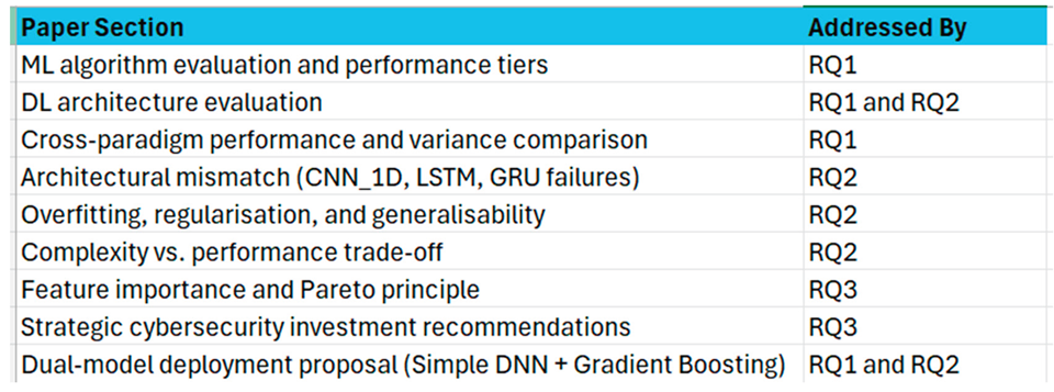
How the THREE questions cover the entire Research?
Research Objectives
Using both traditional machine learning and deep learning methodological approaches, this research aims to develop, evaluate, and systematically compare predictive models for healthcare ransomware threat assessment. As a result of the application of small-scale tabular cybersecurity datasets characteristic of healthcare security operations, comprehensive empirical evidence was established concerning relative performance, operational trade-offs, and practical deployment considerations. Eight distinct machine learning algorithms and eight neural network architectures are evaluated in this comparative investigation to identify optimal approaches for healthcare security systems in which prediction accuracy must be balanced against computational efficiency, infrastructure complexity, model interpretability, and operational robustness.
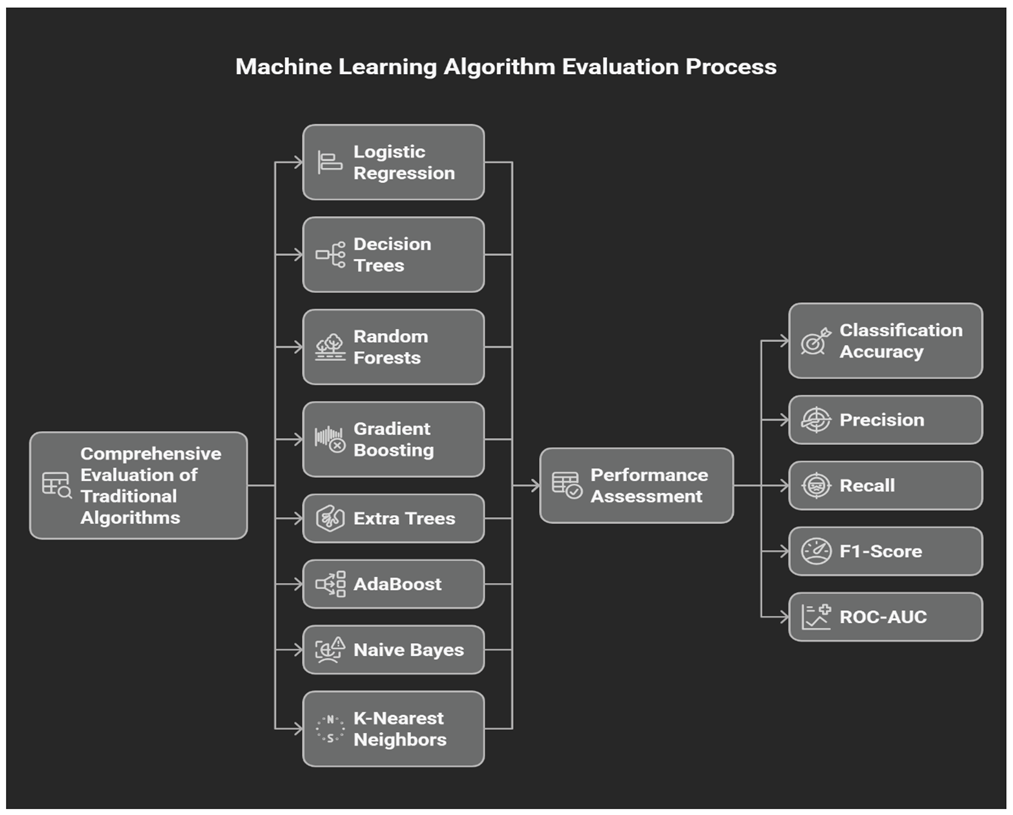
In order to establish performance baselines within the machine learning paradigm, the first specific objective involves a comprehensive evaluation of traditional machine learning algorithms. This includes rigorous assessment of logistic regression as a linear baseline, decision trees that capture hierarchical decision rules through recursive partitioning, and random forests that utilize bootstrap aggregation to reduce variance. Gradient boosting implements sequential error correction using additive modeling, extra trees investigate extreme randomization strategies, AdaBoost tests aggressive reweighting of difficult cases using exponential reweighting, naive Bayes evaluates probability classification under independence assumptions, and K-nearest neighbors examine distance-based pattern matching. To facilitate comprehensive performance assessment and threshold optimization for specific operational requirements, each algorithm is evaluated across five performance dimensions: classification accuracy, precision, recall, F1-score, and ROC-AUC.
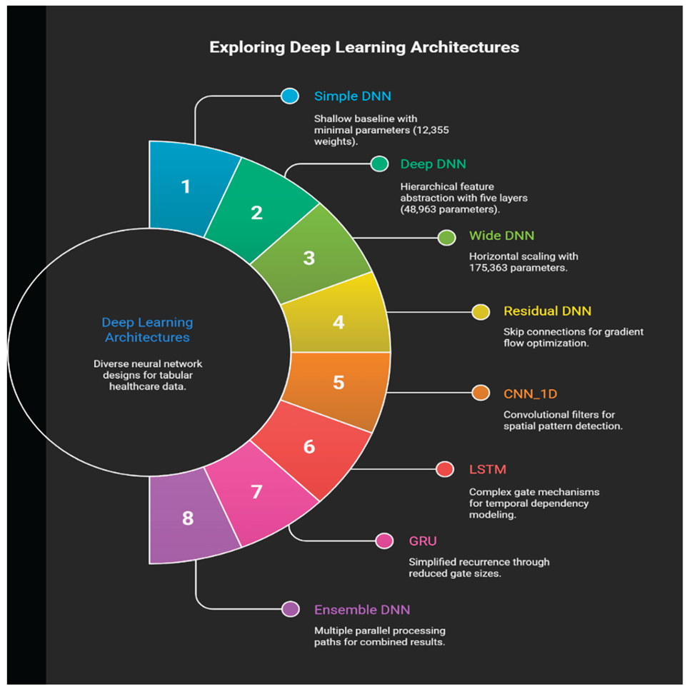
The second objective of this study involves the systematic evaluation of deep learning architectures that represent a variety of neural network design principles. The Simple DNN establishes a shallow baseline with minimal parameters (12,355 weights). Deep DNN testing hierarchical feature abstraction using a five-layer architecture (48,963 parameters) with batch normalization. The wide DNN is examined in terms of horizontal scaling (175,363 parameters). Residual DNN with skip connections for gradient flow optimization. A CNN_1D with convolutional filters is used for detecting spatial patterns in unordered tabular data. An LSTM implementing complex gate mechanisms to model temporal dependency. GRU simplifies recurrence through reduced gate sizes. Ensemble DNN combining multiple parallel processing paths. As a result of this architectural diversity, it will be able to demonstrate how network depth, layer width, skip connections, and recurrent processing have an impact on the performance of tabular healthcare data with limited training data.
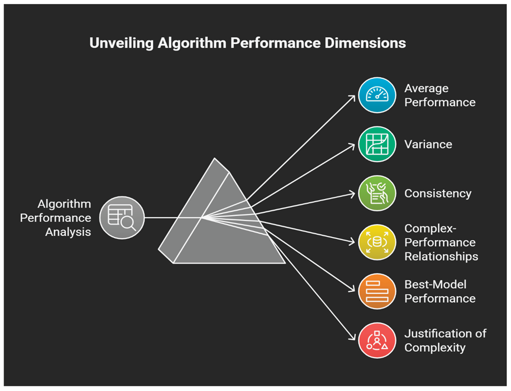
A third objective focuses on systematic cross-paradigm comparative analysis for identifying performance differences, variance patterns, and consistency characteristics that are useful for selecting practical algorithms. As part of this comparison, average performance across algorithmic families are evaluated, variance is quantified through standard deviation analysis, consistency is examined across diverse architectures, complex-performance relationships are assessed to identify diminishing returns, best-model performance is analyzed under optimal configurations, and whether increased infrastructure complexity and operational risk are justified by observed accuracy advantages.
Feature importance analysis is the fourth objective and explores its implications for deployment optimization and strategic security investment. Quantifying individual feature contributions in this analysis, validating concentrated importance patterns consistent with the Pareto principle, and determining optimal feature subsets achieving 90-95% of the full model's performance, examining whether different paradigms uncover similar hierarchies of importance, and recommending which organizational characteristics require priority investment based on these findings.
It is the fifth objective that requires a detailed analysis of model generalization capabilities, overfitting patterns, and the effectiveness of regularization. The analysis includes examining training-validation performance gaps, analyzing cross-validation stability, identifying overfitting signatures in learning curves, examining regularization techniques such as batch normalization and dropout normalization, and determining the optimal architectural complexity based upon dataset size constraints.
Methodology
Data Characteristics
There were 16 distinct variables within the dataset, which were grouped into three analytical dimensions:
Characteristics of the organization (3 features):
- org_type: Categorical nominal variable indicating the classification of healthcare entities (hospitals, clinics, insurance companies, pharmaceutical companies, research laboratories).
- org_size: Variable representing organizational scale (small: 1-50 employees, medium: 50-350 employees, large: 350+ employees)
- monitoring_freq: An ordinal categorical variable indicating the frequency at which cybersecurity monitoring is conducted (daily, weekly, monthly).
Attack Characteristics (6 features):
- attack_date: Recording incident occurrence dates in a temporal variable
- entry_method: Identifying the initial breach vectors (compromised credentials, exploited vulnerabilities, phishing emails, malicious websites, RDP exploits, unsecure remote access) using a categorical nominal variable
- ransomware_infection_rate_(%): A continuous ratio variable quantifying the percentage of compromised systems (0-100%).
- facilities_affected: A discrete count variable that measures the number of impacted organizational sites
- ransomware_incidents: A discrete count variable representing the frequency of historical attacks (0-6 prior incidents)
- cyber_threats_tracked: A categorical variable indicating the sophistication of threat monitoring
Outcome Metrics (7 features):
- recovery_time_(days): a continuous interval variable that measures the duration of operational restoration
- data_restored: a continuous ratio variable measuring the percentage of data successfully recovered (0-100%).
- backup_compromised: The status of the backup system compromise is indicated by a binary Boolean variable
- data_encrypted: a binary Boolean variable indicating whether data encryption has occurred
- data_stolen: a binary Boolean variable indicating the exfiltration of data
- paid_ransom: Boolean binary variable recording ransom payment decisions
Rational for Model Selections
The objective of this study is BINARY CLASSIFICATION: Predicting ransomware attack severity (e.g., Low/Medium/High volume threats, or attack outcomes) based on features of healthcare organizations [64]. There is a requirement for labelled training data where every ransomware incident has a known outcome/class label [64,65]. Consequently, supervised learning is essential when attempting to predict specific target variables (such as ransomware outcomes), learn from historical examples with well-known outcomes, and evaluate accuracy based on ground truth [65]. Unsupervised Machine Learning Models find patterns without labels, which is NOT suitable for tabulated data and consequently make them unsuitable for classification tasks [65,66].
Selection and Exclusion of Supervised machine Learning Models: Rationale and Justification
Why the following models selected?
| Model | Justification | Key benefits |
| Logistic Regression [67] | A closed-form solution for binary classification; an industry standard for scoring medical risks; a reference for the calibration of probabilities |
|
| Decision Tree [68] | Runs non-linear conditional relationships (IF-THEN rules) critical for ransomware scenarios; visualizes decision paths for stakeholder communication; handles mixed feature types |
|
| Random Forest [69] | By combining bagging and feature randomness, decorrelated trees are created that address Decision Tree overfitting; feature importance rankings are robust and critical for identifying organizational weaknesses |
|
| Gradient Boosting (XGBoost) [68] | Using gradient descent to correct sequential errors; state-of-the-art in Kaggle competitions; regularization parameters prevent overfitting |
|
| Support Vector Machine (SVM) [69] | The system maximizes the margin between attack severity classes by utilizing a kernel trick; it is effective in a high-dimensional feature space (17 features); it is robust to outlier ransomware incidents through the use of soft margins |
|
| K-Nearest Neighbors (KNN) [70] | Using instance-based learning preserves local attack patterns; no training phase enables rapid model updates as new ransomware data becomes available; naturally handles multi-modal class distributions. |
|
| Naïve Bayes (Gaussian) [71] | Feature-independent probability classifier; computationally efficient for real-time screening; generates interpretable likelihood ratios |
|
| AdaBoost [68,71] | The adaptive boosting approach focuses on misclassified high-severity ransomware cases, complements Gradient Boosting with different error-weighting mechanisms, and tests the robustness of boosting methods |
|
Why the following models excluded? [72]
| Model | Why Excluded? |
| Linear Discriminant Analysis (LDA) | Redundant - assumes the same Gaussian distributions with equal variance; no advantage over Logistic Regression |
| Perceptron | Inferior with no probabilistic outputs and less stable convergence |
| Rule-based Systems | It is manual and require domain expert rule crafting, and unable to learn from data and inflexible to pattern changes |
| Decision Stumps | It is too simple and single-split trees and lack depth for complex patterns |
| Isolation Forest | Task mismatch. It is designed for anomaly detection, not for supervised classifications |
| CatBoost | It ahs feature overlap-systematic trees offer marginal benefits for data lacking high-cardinality categories |
| HistGradient Boosting | Redundant, histogram binning provides minimal speed-up |
| Linear SVM | Insufficient to analyse, and already tested via logistic regression baseline. It is non-linear kernels essential for attack patterns complexity |
| v-SVM | It is over-complex, and v- parameters offers no practical advantage over C-parameter for binary classifications |
| Radius Neighbors | It is impractical because a fixed radius cannot adapt to changes in attack density across different feature spaces; empty neighborhoods lead to incorrect predictions |
| Nearest Centroid | The use of a single prototype per class leads to the loss of critical attack variation information. |
| Bernoulli / Multinomial Naïve Bayes | Mismatch in feature types - Gaussian NB is appropriate for continuous ransomware metrics (recovery_time, data_restored). |
| Bayesian Networks | It is overengineered - there is a need for domain expertise and larger sample sizes when understanding conditional dependencies |
| LogitBoost | In binary classification, logistic loss provides marginal benefits over exponential loss; however, it adds complexity without offering any clear advantages |
| LPBoost | Theoretical formulations of linear programming are impractical for cyber security systems in production |
Selection and Exclusion of Deep Learning Models: Rationale and Justification
| Model | Justification | Key benefits |
| Simple DNN [74] | This baseline feedforward architecture (128 to 64 to 32 neurons) establishes a minimum level of deep learning performance; tests whether non-linear activation stacking outperforms machine learning; serves as a benchmark for architectural complexity | Overfitting is prevented by a straightforward three-layer design Regularization of batch normalization plus dropout (0.3) Non-linear interactions are captured by ReLU activations Tuning is simplified when hyperparameters are minimal |
| Deep DNN [73,74] | Test of the depth hypothesis - 5 hidden layers (128 to 128 to 64 to 64 to 32) versus 3 layers; investigates whether additional layers can extract hierarchical ransomware patterns (e.g., attack vector to system compromise to recovery failure). | The learning of hierarchical features across five layers A total of 48,963 parameters are available to capture complex patterns Analyzes the diminishing returns of depth for tabular data The assumption that "deeper is better" is validated or refuted The gradient does not vanish due to residual connections |
| Wide DNN [74] | Evaluation of the width hypothesis - three layers with expanded neurons (256 to 256 to 128) compared to a deep narrow architecture; testing whether the wider layers are more effective at capturing feature interactions than the depth layers | The largest model tested consisted of 175,363 parameters Parallel feature combinations are learned by wide layers Analyzes empirically the trade-off between width and depth Contains diverse representations of attack scenarios An alternative to deep networks is gradient flow |
| Residual DNN [75] | Skip connections (inspired by ResNet) address gradient degradation; tests whether identity mappings improve deep architecture training for ransomware prediction; validates shortcut learning hypothesis. | Gradient flow to early layers is enabled by skip connections There are 48,835 parameters that are architecturally innovative Prevents degradation of feature transformations Enhances the performance of deep networks by mitigating vanishing gradients |
| Ensemble DNN [75] | Combining Simple, Deep, Wide, and Residual DNNs by means of averaging; testing whether architectural diversity reduces prediction variance; establishing maximum DL performance through model combination | There are 89,731 total parameters across four sub-models Overfitting is reduced by architectural diversity Predictions for robustness are averaged Analyzes ensemble hypotheses in the context of deep learning Smooths the idiosyncrasies of individual models |
| CNN_1D [76] | Convolutional filters determine whether spatial locality exists in tabular features when they are treated as 1D sequences, and validate or refute the applicability of convolutional architectures beyond the domains of images and signals | Analyzes tabular data to test the spatial pattern hypothesis Detection of local feature groups using convolutional filters By pooling operations, dimensionality is reduced Assesses the portability of the architecture based on the vision Using learned filters, automatic feature extraction can be performed |
| LSTM (Long Short-Term Memory) [76] | This recurrent architecture with gate mechanisms examines the existence of sequential dependencies when features are ordered arbitrarily; evaluates temporal modelling on non-temporal data; challenges the ubiquity assumption of LSTMs | The flow of information is controlled by forget/input/output gates Identifies long-range dependencies (if any) Tests the applicability of RNNs beyond time series data Memory is preserved across features by using a hidden state Validates in a new domain - widely used |
| GRU (Gated Recurrent Unit) [77] | The use of simplified gating (reset and update) as opposed to LSTM's three gates; tests whether the use of simplified recurrent architecture is sufficient for ransomware patterns; computationally efficient RNN variant; compliments LSTM analysis | Faster training with 2 gates compared to 3 gates in LSTMs Overfitting is reduced when fewer parameters are used The hypothesis of minimal gating sufficiency is tested It performs similarly to LSTM in a number of tasks An efficient alternative to sequential modelling |
Why the following models excluded? [78,79]
| Model | Why excluded? |
| Shallow Neural Network (1-2 layers) | Insufficient depth – can NOT capture multi-factor ransomware patterns based on hierarchical feature representations; essentially replicates Logistic Regression |
| Extreme Learning machines | It's hard to compare architectures when hidden layers are randomly initialized |
| Very Deep Networks (10+ layers) | It's too much - the tabular data lacks spatial/temporal structure, and 5000 samples aren't enough to prevent overfitting |
| Highway Networks | It's overly complicated - gating mechanisms add parameters without a clear benefit |
| Ultra-Wide Networks (512+ neurons) | There's overfitting risk - parameter count exceeds sample size and training instability |
| Wide and Deep (Google) | Mismatch between task types - designed for recommendation systems that split memorization from generalization |
| Dense Networks (DenseNet) | The concatenation of all previous layers creates explosive parameter growth; impractical for production cybersecurity |
| Fractal Networks | For classification tasks, recursive structure doesn't have empirical validation |
| Stacking Ensembles | Risk of overfitting - meta-learning with 4 base models and 5000 samples risks learning noise; simple averaging is fine |
| Boosted Neural Networks | Sequential DNN training is computationally expensive; gradient boosting is better for tabular data |
| CNN_2D and CNN_3D | Mismatch in dimensions - 2D convolutions require spatial structure (height x width); tabular data does not include a grid topology |
| Dilated/Atrous Convolutions | The receptive field expansion is unnecessary for 17-feature vectors with no spatial coherence |
| Vanilla RNN | Trainability is compromised by vanishing gradients; LSTM gates are specifically designed to deal with this |
| Bidirectional LSTM | There's no true sequential ordering in tabular data; forward and backward passes process the same unordered stuff |
| Minimal Gated Unit (MGU) | This approach is oversimplified; it lacks empirical validation due to its single gate design |
| Recurrent Highway Networks | It's too complicated - layer-wise gating adds complexity without proving any benefit |
Methodology of Advanced Data Analytics
1.1. The data acquisition and structural framework of the project
This investigation utilized the Healthcare Ransomware Dataset (2024-2025), an open-access repository obtained from Kaggle's data science platform. In selecting the dataset, consideration was given to its comprehensive coverage of ransomware incident characteristics across healthcare organizations, comprising 5,000 simulated attack records that were structured to capture organizational attributes, attack vectors, and outcome metrics. In order to ensure alignment with observed cybersecurity trends while maintaining ethical research standards, the simulation methodology was based on empirical patterns documented in authoritative industry publications, specifically IBM's Cost of a Data Breach Report and Sophos' State of Ransomware in Healthcare. There were 16 distinct variables organized into three analytical dimensions in the dataset. These dimensions include: organizational characteristics including organization type, organization size, and monitoring frequency; attack characteristics encompassing attack date, entry method, ransomware infection rate, facilities affected, ransomware incidents, and cyber threats tracked; and outcome metrics involving recovery time, data restored percentage, backup compromised status, data encrypted status, data stolen status, and ransom payment status. To assist in guiding subsequent analytical procedures, variables were classified by data type, with continuous ratio variables used for percentage-based metrics, discrete count variables used for facility and incident tallies, categorical nominal variables used for unordered classifications, categorical ordinal variables used for ranked categories, binary Boolean variables used for binary decision points, and temporal datetime variables used for chronological data.
1.2 Protocol for Data Quality Assessment
Prior to conducting substantive analyses, a comprehensive five-dimensional data quality assessment framework was implemented to ensure the validity and reliability of the analysis. During the consistency validation phase, data type conformity was verified to ensure all values within each feature adhered to expected formats. A thorough review of the encoding consistency of categorical variables was conducted in order to eliminate potential typographical variations or case inconsistencies that might artificially fragment categories. Validity assessments were conducted on continuous variables, ensuring that percentage-based metrics remained within the logical range [0,100] and that count variables retained non-negative integer values. By confirming that attack_date values fell within plausible chronological boundaries for the observation period of 2024, the temporal validity of the data was verified. As part of the distributional plausibility evaluation, preliminary distribution assessments were used to determine if observed patterns aligned with domain knowledge and established cybersecurity research paradigms, emphasizing the distinction between potential data entry errors and legitimate extreme situations.
1.3 Statistical procedures for descriptive analysis
All continuous and discrete numerical variables were analysed using comprehensive descriptive statistics, including measures of central tendency (mean, median, mode), dispersion (standard deviation, interquartile range, coefficient of variation), and distributional shape (skewness, kurtosis). To characterize the distribution of observations across categories for categorical variables, frequency distributions and relative proportions were calculated.
1.4 Correlation Analysis
A Pearson product-moment correlation coefficient was computed for each pairwise combination of continuous variables for each pair of continuous variables. Based on conventional thresholds, the correlation strength was interpreted as follows: below 0.30 was classified as weak, 0.30 to 0.70 was classified as moderate, and > 0.70 was classified as strong. An annotation heatmap was created based on the correlation matrix, and this was visualized as the correlation matrix.
1.5 A framework for detecting and analysing outliers
In order to identify outliers based on the interquartile range, Tukey's fence method was applied to five continuous variables. It was determined that mild outliers should be multiplied by 1.5, whereas extreme outliers should be multiplied by 3.0. The results were visualized using box plots, and each flagged outlier was interpreted contextually rather than automatically being removed.
1.6 Data analysis and visualisation of categorical distributions
For each categorical variable, frequency distributions and proportional analyses were carried out. The ratios between selected category pairs were calculated in order to identify dominant patterns of targeting or occurrence between the two categories. An analysis of compound patterns across multiple categorical variables simultaneously was carried out using cross-tabulations, and the results were visualized using bar graphs to display the results.
1.7 Characterization of distribution shapes
To characterise the distributional shape of each continuous variable, frequency histograms were constructed using adaptive binning strategies in order to generate frequency histograms. There was a visual inspection of each histogram for modalities, symmetry, and tail behavior associated with it.
1.8 The implementation of analytical software
The whole data engineering, statistical computation, and visualization was carried out in Python 3.9 or higher with the use of pandas, NumPy, SciPy, Matplotlib, and Seaborn packages. A colourblind-accessible palette was used in all visualisations made at 300 DPI with all visualisations being produced at 300 DPI.
Methodology of Machine Learning Model Selection
It was necessary to develop a comprehensive machine learning framework for predicting ransomware outcomes for healthcare organizations in order to model the complex, multifaceted relationships inherent in cybersecurity incidents. Healthcare Ransomware Dataset, containing 5,000 simulated records with 14 features representing organizational attributes, attack vectors, and technical outcomes, presented a classification challenge requiring algorithms capable of handling non-linear relationships, feature interactions, and hierarchical decision boundaries. In selecting eight unique machine learning algorithms, performance baselines were established, algorithmic assumptions were evaluated against dataset characteristics, and optimal prediction methods were identified to ensure patient safety during ransomware-induced operational disruptions during mission-critical healthcare security applications.
2.1 Logistic Regression
For the purpose of establishing minimum acceptable performance thresholds and quantifying the degree to which ransomware outcomes can be distinguished linearly, Logistic Regression was used as the foundational baseline model. Modeling class probabilities using the sigmoid activation function is the objective of this algorithm:
P(y=1|x) = 1/(1 + e^(-θᵀx))
θ represents the learned coefficient vector while x represents the feature vector consisting of organizational and technical attributes. In this model, parameters are optimized by maximizing the log-likelihood function:
h_θ(x) represents the hypothesis function. Logistic regression is important in determining whether simple linear combinations of features such as organization size, recovery time, and data restoration percentages can adequately predict ransomware severity, or whether more sophisticated non-linear models are required to address the problem. Moreover, it provides valuable insights into individual feature contributions, making it essential for understanding baseline relationships before applying complex ensemble methods.
L(θ) = Σ[y_i log(h_θ(x_i)) + (1-y_i)log(1-h_θ(x_i))]
2.2 Decision Trees
A recursive binary partitioning method was used to capture hierarchical decision rules and non-linear patterns using Decision Trees. As a result of the algorithm, splits are constructed based on information gain or Gini impurity:
Gini = 1 - Σp_i²
(p_i represents the proportion of samples at each node that belong to class i).
In order to maximize information gain, it is best to split the selection:
IG(D,A) = Entropy(D) - Σ(|D_v|/|D|)Entropy(D_v)
A is a candidate splitting attribute (where D represents a dataset subset and A represents a dataset subset).
As a result of their ability to naturally model conditional relationships, Decision Trees are essential in ransomware prediction
"IF organization_size = medium AND backup_compromised = yes, recovery time will exceed 100 days," which cannot be represented by linear decision boundaries.
This algorithm is particularly relevant in scenarios where organizational characteristics interact through conditional dependencies rather than additive effects. The tree structure resembles the logical decision-making process security analysts use to assess ransomware threat severity.
2.3 Random Forests
Using bootstrap aggregation (bagging), Random Forests extend the capabilities of a single Decision Tree by creating an ensemble of N trees trained on random subsamples with random feature selections.
f(x) = (1/N)Σf_i(x)
(where f_i represents an individual prediction in the tree).
At each split, each tree utilizes a random subset of features (typically p features for p total features). The final predictions are determined by majority vote based on the scores of the individual trees in the ensemble. In healthcare organizations, there is substantial heterogeneity in terms of size, infrastructure maturity, and security posture, creating high variance in individual decision tree predictions. Through ensemble averaging, Random Forest reduces overfitting while still capturing complex feature interactions, making it particularly suitable for datasets containing different organizational profiles (hospitals, clinics, and research laboratories) with distinct vulnerability patterns requiring multiple independent decision boundary perspectives.
2.4 Gradient Boosting
Using gradient boosting, sequential error correction is implemented through additive modeling.
F_m(x) = F_(m-1)(x) + γ_m h_m(x)
(where F_m is the cumulative model at iterations m, while h_m denotes a weak learner fitted to the negative gradient of the loss function, and γ_m controls the learning rate).
The algorithm minimizes L iteratively by:
h_m = argmin_h Σ L(y_i, F_(m-1)(x_i) + h(x_i))
The aim of each successive tree is to correct residual errors from previous iterations.
The need for this approach is critical when it comes to ransomware datasets since certain outcomes may be systematically difficult to classify, such as medium-sized organizations with adequate monitoring, but compromised backups that suffer catastrophic recovery times. Due to gradient boosting's iterative refinement, the model may be able to acquire superior discrimination capabilities over parallel ensemble methods that treat all patterns equally.
2.5 Extra Trees
Unlike Random Forest, Extra Trees (Extremely Randomized Trees) employ enhanced randomization by selecting both random feature subsets and random split thresholds.
Split(x,θ) = x < θ_random
(θ_random is drawn from a uniform distribution across the feature's observed range rather than from a set of split points).
The ensemble prediction follows:
f(x) = (1/N)Σf_i(x) (with maximum randomization).
An important aspect of this algorithm is its ability to test whether extreme randomization reduces overfitting to training-specific noise patterns, such as the 21 low-infection outliers and 30 extreme 120-day recovery cases identified in the dataset. By avoiding overfitting to dataset-specific anomalies, Extra Trees' aggressive variance reduction may outperform Random Forest's controlled randomization when ransomware outcomes contain substantial stochastic variation.
2.6 AdaBoost
In AdaBoost (Adaptive Boosting), exponential loss minimization is achieved by reweighting samples in an iterative manner.
α_t = (1/2)ln((1-ε_t)/ε_t)
(where ε_t is the weighted error rate for weak classifier t)
The sample weights update exponentially as follows:
w_i^(t+1) = w_i^t exp(α_t · 𝟙(h_t(x_i) ≠ y_i))
In other words, it forces subsequent classifiers to concentrate on instances that have been misclassified previously.
As a result of the final prediction, weak learners are grouped as follows:
H(x) = sign(Σα_t h_t(x)) (weighted by their individual accuracy).
AdaBoost's relevance to ransomware prediction is derived from the hypothesis that certain organizational profiles may be systematically difficult to classify using standard methods, such as organizations with paradoxical characteristics such as high monitoring frequency and poor backup practices. According to the concept of aggressive reweighting, the model is theoretically capable of developing specialized decision boundaries for these challenging cases, provided that they represent genuine patterns rather than noise or outliers.
2.7 Naïve Bayes
By applying Bayes' theorem and assuming feature independence, Naive Bayes applies probabilistic classification:
P(y|x) = P(y)P(x|y)/P(x) = P(y)∏P(x_i|y)
(Treating features x_i as being conditionally independent with respect to class y).
While this algorithm simplifies the assumption, it is still important for ransomware prediction because it provides a probabilistic baseline that reveals whether or not features interact in a meaningful way. Despite the assumption of independence, Naive Bayes can perform competitively, suggesting features play an additive role in ransomware severity. On the other hand, poor performance establishes the necessity of models that can capture the interaction between features, as well as the fact that variables such as organizational size fundamentally influence the impact of other factors such as backup compromises or monitoring frequencies on recovery outcomes.
2.8 K-Nearest Neighbour (KNN)
KNN algorithm implements instance-based classification without explicitly constructing a model:
ŷ = mode{y_i : x_i ∈ N_k(x)}
N_k(x) identifies k nearest training samples based on Euclidean distance
Euclidean Distance: d(x,x_i) = √(Σ(x_j - x_ij)²)
The classification process is based on a majority vote among these neighbors. An important application of KNN is its ability to test whether ransomware outcomes exhibit local similarity patterns or whether organizations with similar characteristics (measured by distance in a fourteen-dimensional feature space) experience similar attack outcomes. As a diagnostic tool, this algorithm also indicates whether the dataset's 14 features create sparse feature spaces that render distance-based similarity unreliable, indicating that dimensionality reduction or feature selection strategies are needed.
In order to assess model performance across multiple dimensions, five comprehensive metrics were employed.
The accuracy of the measurement is based on the following equation: Accuracy = (TP+TN) / (TP+TN+FP+FN).
Positive prediction reliability is quantified by precision: Precision = TP/(TP+FP).
Captured recall sensitivity can be calculated as follows: Recall = TP/(TP+FN).
Using the F1-score harmonised precision recall formula, F1 = 2(Precision×Recall)/(Precision+Recall).
As ROC-AUC measures the area under the receiver operating characteristic curve, it provides threshold-independent performance evaluation essential for healthcare applications requiring flexible risk stratification.
Cross-validation standard deviation quantified prediction stability across different data splits, with a tighter variance indicating more reproducible real-world performance essential for mission-critical ransomware prediction that supports medication safety and operational continuity.
Methodology for selecting deep learning models
The deep learning methodology for cyber threat volume prediction in healthcare organizations required a systematic evaluation of eight distinct neural network architectures, each designed to test different hypotheses about feature representation, pattern extraction, and generalization capabilities on tabular healthcare cybersecurity data. Operated on TensorFlow 2.19.0 without GPU acceleration. A pipeline was developed to process the Healthcare Ransomware Dataset to target a fundamentally different prediction task from that of previous machine learning models. Organizations are subdivided into three categories of cyber threat volume ('1-50 threats', '50-350 threats', and '350+ threats') by analyzing 14 preprocessed features consisting of numerical attributes (organization size, recovery time, facilities affected) and categorical attributes (organization type, entry method, monitoring frequency). The dataset utilized a conservative 60-20-20 split (3,000 training, 1,000 validation, 1,000 testing samples) to provide robust validation sets essential for detecting overfitting in neural networks, which exhibit greater memorization tendencies than traditional machine learning algorithms on limited datasets.
As part of feature preprocessing, a scaling operation was performed either by standardizing (zero mean, unit variance) or by normalizing (0-1 range) in order to ensure features of disparate magnitude (organization size ranging 1-1,000 versus infection rate 0-1) contribute equally to gradient-based weight updates, thus preventing the network from biasing towards high-magnitude features and accelerating convergence by maintaining gradients within numerically stable ranges. The purpose of this preprocessing is to address the fundamental challenge of training neural networks on heterogeneous tabular data, in which unscaled features can cause optimization instability and result in prolonged training times.
3.1 Simple DNN
The Simple DNN (Deep Neural Network) was implemented as a lightweight three-layer architecture with progressive dimensionality reduction (128 neurons to 64 neurons to 32 neurons) followed by softmax output for classification into three classes.
The forward propagation is as follows:
h₁ = ReLU(W₁x + b₁), h₂ = ReLU(W₂h₁ + b₂), ŷ = softmax(W₃h₂ + b₃), where ReLU(z) = max(0,z) introduces non-linearity and softmax(z_i) = exp(z_i)/Σexp(z_j) produces class probabilities.
As part of the training process, strategic dropout layers (typically 0.3-0.5) apply multiplicative noise:
h_dropped = h × Bernoulli(1-p)/(1-p)
Zeroing activations randomly in order to prevent co-adaptation and reduce overfitting.
The importance of this architecture lies in determining whether shallow networks with minimal parameters (12,355 total) can effectively capture cyber threat patterns when strong feature engineering provides meaningful input signals. Specifically, this study will investigate whether architectural simplicity and quality features can be more effective than complex models when applied to small datasets where parameter-to-sample ratios are critical for generalizing results.
3.2 Deep DNN
As the Deep DNN is expanded to five layers (256 neurons to 128 neurons to 64 neurons to 32 neurons to 3 neurons), batch normalization is applied after the first three dense layers in order to stabilize the training process through the reduction of internal covariate shifts.
A batch normalization transforms activations as follows:
x̂ = (x - μ_B)/√(σ²_B + ε), y = γx̂ + β
Where μ_B and σ²_B represent mini-batch mean and variance, while γ and β are learnable scale and shift parameters.
In the architecture, 48,963 parameters are used to see if increasing depth allows hierarchical feature abstraction. Lower layers detect simple patterns (organization size categories), middle layers combine features (size + backup status), and upper layers learn complex decision boundaries to classify threats. A key reason for this model's importance is to figure out if depth makes sense in tabular cyber threat data like it does in computer vision, or whether the limited training samples (3,000) make it hard to exploit additional layers, validating the data vs. depth trade-offs fundamental to neural architecture selection.
3.3 Wide DNN
To test if width enables parallel processing of different feature combinations within single layers compensates for limited training data differently than depth, Wide DNN implemented extreme horizontal scaling (512 neurons to 256 neurons to 128 neurons to 3 neurons) with 175,363 parameters.
The forward path maintains a shallow structure but massively expands capacity:
h₁ = ReLU(W₁x + b₁) where W₁ ∈ ℝ^(512×14) (creating 512 parallel feature detectors).
The significance of this architecture lies in the ability to distinguish width-based overfitting from depth-based overfitting. Furthermore, looking at whether broad layers that evaluate multiple feature interactions simultaneously (organization size, monitoring frequency, backup status, entry method) can recognize threats better than sequential hierarchical processing, especially on datasets where threat patterns emerge from combinatorial feature relationships rather than hierarchical abstractions.
3.4 Residual DNN
In Residual DNN, skip connections were incorporated that were influenced by ResNet architectures:
h_l = ReLU(F(h_(l-1), W_l) + h_(l-1))
In this case, F represents the residual mapping and identity shortcuts bypass dense layers.
It is theorized that this design can solve the problem of vanishing gradients in very deep networks by means of gradient highways:
∂L/∂h_(l-1) = ∂L/∂h_l × (∂F/∂h_(l-1) + I) (allowing gradients to flow through identity paths).
The architecture's importance lies in testing whether residual connections revolutionary for 100+ layer computer vision models work in shallow 5-layer healthcare tabular networks. Using gradient flow mechanisms designed for extreme depth transfer and also to see if they're better than those with moderate depths with different data structures (images versus tabular features).
3.5 CNN_1D
In CNN_1D, one-dimensional convolutional filters were applied to tabular features treated as sequential data in the following manner:
h = ReLU(W * x + b)
Where * denotes a convolution operation [W * x]i = Σ_k W_k × x(i+k) scanning local feature windows.
As part of this architecture, spatial pattern detection is tested for image pixels and time-series timestamps and transferred to unordered tabular features, as well as whether treating organization size, recovery time, and backup status as a sequential feature enables learning meaningful local patterns despite features lacking inherent ordering, thereby validating or refuting CNN's applicability beyond explicitly sequential domains.
3.6 LSTM
An LSTM (Long Short-Term Memory) implemented a recurrent architecture with gating mechanisms, as follows:
f_t = σ(W_f[h_(t-1), x_t] + b_f) (forget gate), i_t = σ(W_i[h_(t-1), x_t] + b_i) (input gate), C̃_t = tanh(W_C[h_(t-1), x_t] + b_C) (candidate cell), C_t = f_t ⊙ C_(t-1) + i_t ⊙ C̃_t (cell state update), o_t = σ(W_o[h_(t-1), x_t] + b_o) (output gate), h_t = o_t ⊙ tanh(C_t) (hidden state).
Where σ denotes sigmoid function and ⊙ element-wise multiplication.
The importance of this architecture lies in seeing if memory mechanisms that are designed for temporal dependencies (previous timesteps affecting future predictions) help process static tabular cyber threat features. By treating features as sequences, hidden state accumulation can capture relationships among organizationally-related attributes even if there's no true temporal structure.
3.7 GRU
Recurrent processing has been simplified by the GRU (Gated Recurrent Unit), which reduces the gating process as follows:
r_t = σ(W_r[h_(t-1), x_t]) (reset gate), z_t = σ(W_z[h_(t-1), x_t]) (update gate), h̃_t = tanh(W[r_t ⊙ h_(t-1), x_t]) (candidate activation), h_t = (1-z_t) ⊙ h_(t-1) + z_t ⊙ h̃_t (final hidden state).
With two gates versus LSTM's three, GRU tests whether architectural simplification reducing parameters while maintaining recurrent capability enhances efficiency for tabular data where full LSTM complexity may not be necessary. On limited healthcare cybersecurity samples, streamlined sequential processing was evaluated to determine whether streamlined sequential processing better balanced expressiveness and overfitting prevention.
3.8 Ensemble DNN
Ensemble DNN used multiple branches of parallel processing with three independent pathways: narrow-deep (128 neurons to 64 neurons), wide-shallow (256 neurons to 128 neurons), and direct (64 neurons), which were concatenated prior to final classification:
h_concat = [h_narrow; h_wide; h_direct], ŷ = softmax(W_final × h_concat + b_final).
The significance of this architecture is that it tests whether different feature representations can simultaneously learn from different inductive biases (depth for abstraction, width for combinations, directness for linear relationships). Furthermore, it enables ensemble averaging benefits for single-model training, so it can see if parallel paths capture complementary cyber threat patterns that single-pathway architectures miss, especially for datasets with multiple feature interaction types.
Entropy
During model training, categorical cross-entropy loss was employed:
L = -Σ_i Σ_c y_(i,c) log(ŷ_(i,c))
Optimised using Adam's optimizer, which combines momentum and adaptive learning rates:
m_t = β₁m_(t-1) + (1-β₁)∇L, v_t = β₂v_(t-1) + (1-β₂)(∇L)², θ_t = θ_(t-1) - α(m_t/√(v_t + ε)),
In order to prevent unnecessary training epochs and overfitting, ReduceLROnPlateau calls to schedule learning rates and monitor validation loss early in the training process.
A comprehensive evaluation used accuracy, precision, recall, ROC-AUC metrics, confusion matrices, and learning curves to detect overfitting signatures (training-validation divergence), assess performance across three threat volume categories, and validate generalization capabilities needed to deploy healthcare cybersecurity in production
Comparative Analysis Methodology for Models Based on Deep Learning and Machine Learning
The comparative analysis methodology used a systematic evaluation framework to assess the relative strengths, weaknesses, and operational trade-offs of traditional machine learning and deep learning approaches for predicting healthcare cyber threats. This cross-paradigm comparison addresses a fundamental research question in applied cybersecurity analytics: whether neural network architectures justify their increased computational complexity and infrastructure requirements when operating on structured tabular healthcare data with limited sample sizes (5,000 records) over established tree-based and probabilistic algorithms. This evaluation framework compares eight machine learning algorithms (Logistic Regression, Decision Tree, Random Forest, Gradient Boosting, Extra Trees, AdaBoost, Naive Bayes, K-Nearest Neighbors) with eight deep learning architectures (Simple DNN, Deep DNN, Wide DNN, Residual DNN, CNN_1D, LSTM, GRU, Ensemble DNN). Aim of this evaluation is to establish empirical evidence for algorithm selection in production healthcare security operations where prediction accuracy, computational efficiency, and operational reliability must be balanced with infrastructure complexity and maintenance requirements. Methodology for the analysis of feature importance Prior to model comparison, feature importance analysis was conducted in order to determine the hierarchical contribution of input variables to prediction power, enabling interpretation of which organizational and technical attributes have the greatest influence on cyber threat volume classification. In tree-based machine learning models, feature importance is determined by the mean decrease in impurity across all splits: Importance(f) = Σ_t [p(t) × ΔI(t)] where p(t) measures the proportion of samples reaching node t and I(t) indicates the reduction in impurities (Gini or entropy decrease) achieved by splitting on feature f at that node. Based on the cumulative importance normalized to 100%, this metric quantifies how frequently and effectively each feature (organization size, recovery time, data restoration, infection rate, etc.) participates in decision boundary construction across the ensemble. In this study, 14 input features were categorized hierarchically to identify dominant predictors versus marginal contributors, thereby examining whether ransomware prediction reveals concentrated feature importance (80% of prediction power is contributed by the top 20% of features using the Pareto principle) versus distributed importance (all features contribute roughly equally).
In addition to ranking features, the feature importance methodology serves a number of critical purposes. Specifically, it tests whether deep learning's automatic feature extraction wins over machine learning's explicit feature engineering and if neural networks discover non-obvious feature interactions that tree-based methods miss. The method also establishes baseline expectations for performance. Datasets with highly concentrated importance (a single feature dominates) are more likely to favor simple models, whereas datasets with distributed importance are more likely to benefit complex architectures capable of integrating a variety of weak signals. Additionally, importance analysis informs deployment monitoring strategies by identifying which features require high-quality data collection (dominant predictors) versus which are tolerated with missing or noisy values (marginal contributors), enabling resource-efficient data governance in healthcare environments with heterogeneous information systems.
A framework for cross-paradigm performance comparisons
To establish an understanding of classification capability, discrimination capability, and precision-recall tradeoffs, the comparative methodology used five-dimensional performance assessments evaluating accuracy, precision, recall, F1-score, and ROC-AUC across sixteen models (eight ML, eight DL). Using this multi-metric approach, models achieving high accuracy through majority class bias are penalized by low F1 scores, while models with excellent ROC-AUC and poor accuracy are revealed as having problems with probability calibration. For tabular cyber threat data, this framework determines whether deep learning's gradient-based optimization and hierarchical representations offer fundamental advantages over machine learning's closed-form solutions and ensemble aggregation, or if limited training samples (3,000) and a poor feature engineering quality undermine neural network benefits observed in large-scale computer vision and natural language processing applications.
With average performance aggregation across algorithms, all eight ML models and all eight DL models can be compared independently of algorithm selection. By calculating mean accuracy, F1-score, and ROC-AUC separately, we can answer whether neural networks outperform traditional methods as a class. Mean comparisons are accompanied by statistical variance analysis that calculates the standard deviation of performance metrics within each paradigm to quantify consistency. Low variance indicates robust performance across diverse architectures (any reasonably designed neural network will achieve similar accuracy), while high variance indicates sensitivity to algorithm selection (picking the wrong machine learning algorithm severely degrades performance).
Analyzing the relationship between complexity and performance
The methodology systematically varied architectural complexity within deep learning models measured by total trainable parameters ranging from 12,355 (Simple DNN) to 175,363 (Wide DNN) in order to establish empirical relationships between model capacity and classification performance on limited healthcare tabular data. This analysis tests the fundamental hypothesis that increased complexity enables superior pattern learning versus a competing hypothesis that excess parameters relative to training samples induce overfitting that reduces generalization (parameter-to-sample ratios from 4.1:1 to 58.5:1). On a six-point scale, complexity levels were categorized along with parameter counts, allowing visualization of performance plateaus at which additional architectural sophistication decreases performance.
Linear models (Logistic Regression) occupy the simplest tier in machine learning complexity, while single trees (Decision Tree) have moderate complexity, and ensemble methods (Random Forest, Gradient Boosting) achieve maximum complexity by aggregating hundreds of individual models. A cross-paradigm complexity comparison is conducted to determine whether ML's discrete complexity tiers (levels 1-2) versus DL's continuous complexity spectrum (levels 2-6) present different performance-complexity trade-offs, as well as whether neural networks require specific minimum complexity thresholds to achieve competitive performance or if simpler architectures are sufficient for structured healthcare data analysis. An analysis of variation at each level of complexity quantifies performance stability. A tight clustering indicates robust architectures that are generally applicable, whereas a wide spread reveals a high degree of sensitivity to hyperparameters and training randomness.
An analysis of statistical comparisons and deployment strategies
For the statistical comparison, descriptive analytics were used to calculate the mean, standard deviation, minimum, and maximum values for each performance metric across algorithm families, allowing for a quantitative assessment of central tendency and variability. Within paradigms, range analysis (maximum - minimum) quantifies the performance ceiling and floor, thereby establishing the worst-case and best-case scenarios for each approach. As part of the methodology, best-performing models from each paradigm were explicitly compared to establish achievable performance upper bounds, while acknowledging that production deployments may not achieve optimal configurations. This methodology evaluates operational trade-offs beyond pure accuracy, taking into account infrastructure requirements (TensorFlow/Keras dependencies for deep learning versus scikit-learn simplicity for machine learning). Computational latency (cpu-efficient gradient boosting for real-time queries versus GPU-accelerated neural networks for batch processing), interpretability requirements (tree-based feature importance for security analyst auditing versus black-box neural representations), and fault tolerance requirements (redundant prediction pipelines with ML fallback in case the deep learning infrastructure fails). Using this pragmatic evaluation framework, it is recognized that 1-2 percentage point accuracy differences must be weighed against operational complexity in mission-critical healthcare cybersecurity where prediction system downtime directly impacts the safety of patients during ransomware attacks.
Initial Experiments of the Thesis
I decided to use Healthcare Ransomware Dataset (2024-2025) Open Access. Healthcare Ransomware Dataset contains 5000 simulated records that are structured to capture the multifaceted impact of ransomware incidents on healthcare organizations. Every record represents a unique attack scenario, incorporating variables such as organization type and size, monitoring frequency, infection rates, backup compromise, recovery times, ransom payments, and data restoration percentages. The dataset presents a holistic view of how ransomware affects hospitals, clinics, and research laboratories by including both organizational attributes and technical outcomes. Based on industry reports such as IBM's Cost of a Data Breach and Sophos' State of Ransomware in Healthcare, the simulated data is aligned with observed trends in healthcare cybersecurity.
Ransomware attacks are a big problem for healthcare institutions, so the dataset is really valuable. Healthcare providers need access to patient data to provide critical care, and medical records contain highly sensitive personal and financial info. The urgency makes them more likely to pay ransoms, while legacy systems and unpatched vulnerabilities make them more vulnerable. By modelling attack entry methods like phishing, exploited vulnerabilities, and compromised credentials, and outcomes like patient care delays, financial losses, and reputational damage, the dataset captures these realities. Datasets like this allow researchers to explore causality and resilience by encoding relationships like compromised backups and longer recovery times.
It is important to apply machine learning and deep learning models to this dataset for a number of reasons. Firstly, structured features allow for predictive modelling: algorithms can be trained to predict recovery times, classify attack severity, or predict the likelihood of ransom payment. Second, anomaly detection models can identify unusual patterns in infection rates or entry methods, which can support proactive defence strategies. The third benefit of deep learning architectures is the ability to uncover complex, non-linear relationships between variables, such as how monitoring frequency influences infection rates and recovery outcomes. To design intelligent intrusion detection systems and resilience frameworks tailored to healthcare environments, these insights are essential.
Additionally, the dataset supports benchmarking and reproducibility. ML/DL architectures such as random forests, gradient boosting, CNNs, or LSTMs may be compared on the same dataset, ensuring that proposed solutions are evaluated consistently. In healthcare, patient safety depends on reliable and validated cybersecurity measures. As a result of applying machine learning and deep learning to the Healthcare Ransomware Dataset, the research community can move beyond descriptive analysis to predictive and prescriptive solutions, ultimately strengthening the resilience of healthcare systems against one of the fastest-growing cyber threats.
For full access to the dataset, please click at this link: Healthcare Ransomware Dataset
Results
Part 1: Data Engineering & Advanced Data Analysis
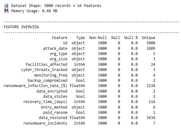
An overview of the Healthcare Ransomware Dataset's structure, features, and quality metrics. There are no missing values (0.0% null) across all 5,000 records and 16 features, eliminating imputation and ensuring reliable model training. Continuous features show high variability (3,238 unique infection rates, 3,436 unique data restoration values) and categorical features demonstrate appropriate stratification (5 organization types, 3 size categories, 3 threat levels).
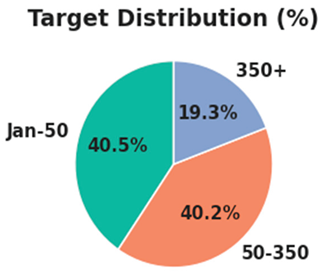
Balanced Vulnerability Across Organization Sizes: According to the target distribution, ransomware threats are nearly equally distributed among small (Jan-50: 40.5%), medium (50-350: 40.2%), and large organizations (350+: 19.3%). There is no difference between smaller and larger health care facilities in terms of vulnerability, which challenges the assumption that only large hospitals are the main targets of attackers.
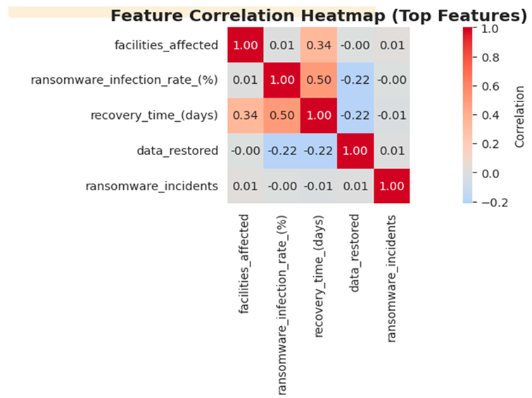
An analysis of correlation heatmaps revealing bivariate relationships among the top predictive features in the ransomware dataset, with red colors indicating positive correlations (features increase together), blue colors indicating negative correlations (one increases while the other decreases), and white/neutral colors indicating near zero correlations (no linear relationship). There is a strong positive correlation (0.50, dark red) between infection rate and recovery time, indicating that the severity of the infection has an exponential effect on recovery time. It is evident from the negative correlations (-0.22, blue) between data_restored and both metrics that severe infections and prolonged recovery adversely affect data restoration success; critically, ransomware_incidents exhibits near-zero correlations (white cells) with all features, indicating organizations fail to learn from repeated attacks and remain equally vulnerable regardless of breach history.
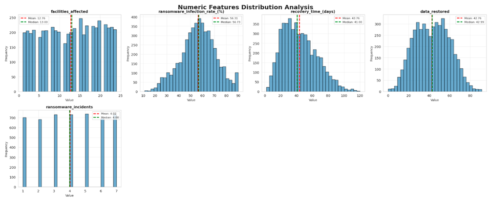
An analysis of five continuous numeric features across 5,000 ransomware incidents, displaying their frequency patterns and central tendency (mean/median). Healthcare is facing a sustained operational crisis with attackers consistently compromising 56% of systems (tight normal distribution). Recovery periods averaged 44 days with catastrophic outliers extending to 120 days, and data restoration averaged only 50%, indicating permanent loss of half of all data regardless of recovery efforts. The uniform 12-13 facilities affected pattern proves ransomware spreads systemically across integrated healthcare networks, whereas the discrete ransomware_incidents distribution (median 4 attacks) and notable peaks at values 1, 3, 4, 6, 7 (but absent from value 2) suggest quarterly targeting cycles where attackers consistently return to previously compromised organizations.
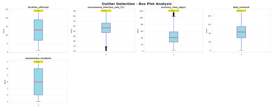
A box plot analysis is performed using Tukey's fence method to identify outliers across five continuous ransomware features, with boxes representing interquartile ranges (25th-75th percentile), red lines indicating medians, whiskers extending beyond non-outlier boundaries, and points beyond whiskers indicating extreme values. Significant Result: 21 low-infection-rate outliers (<20%) prove early detection can keep compromises to a minimum, but 30 catastrophic disaster recovery outliers (100-120+ days) show inadequate backups pose existential risks. A critical finding is that there are no outliers among facilities_affected, data_restored, or ransomware_incidents, indicating a uniform systemic failure where ransomware consistently spreads across 7-19 facilities. All organizations lose over 50% of their data regardless of the response strategy they employ (no high performers are able to restore more than 60% of their data). In the healthcare industry as a whole, all organizations suffer chronic repeat victimization (2-6 incidents), with no organization being able to prevent attacks, which demonstrates the complete failure of network segmentation and backup strategies.
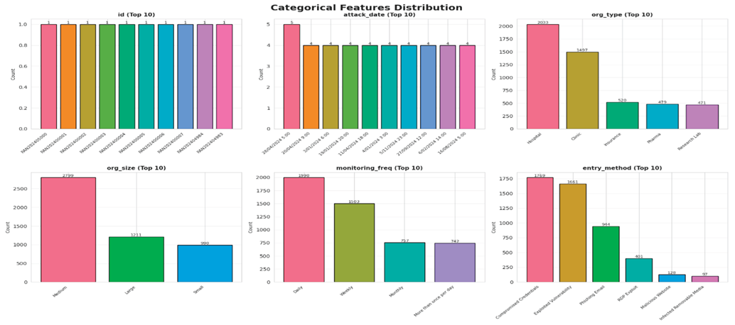
The analysis shows frequency counts across six discrete variables (ID, attack_date, organization_type, organization_size, monitoring_freq, entry_method) with color-coded bars representing different categories within each variable. There is a 2:1 disproportionate targeting of hospitals (2,033 attacks compared to 1,497 clinics) as a result of a higher ransom capacity and critical care disruption leverage. Consequently, medium-sized organizations suffer the most attacks (2,799 versus 1,211 large and 990 small), representing the "Goldilocks Zone" vulnerability with inadequate enterprise security, but sufficient ransom potential. It is important to note that 69% of breaches occur as a result of just two methods: compromised credentials (36%) and exploited vulnerabilities (33%). Observing the daily monitoring paradox, organizations with daily monitoring experience 40% of attacks versus 30% with weekly monitoring, suggesting detection bias rather than prevention effectiveness. Accordingly, ransomware threatens healthcare continuously year round without seasonal patterns enabling predictable security adjustments. Its uniform temporal distribution across attack dates demonstrates that ransomware threatens healthcare constantly year-round.
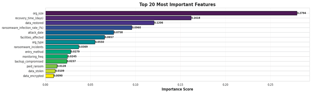
The horizontal bar chart illustrates feature importance scores ranked from highest to lowest, with colors ranging from dark purple (critical features) to blue, cyan, green, and yellow (minimal features). The extreme hierarchical concentration reveals that org_size (0.2794) dominates as one of the most important predictors, nearly 1.73x greater than recovery_time (0.1618), and accounting for more than the next four features combined. As a result, the top 3 features (org_size, recovery_time, data_restored) account for 56% of the total prediction power while representing only 21% of all features. This illustrates a clear Pareto distribution, in which organizational preparedness characteristics significantly outweigh attack specifics. Despite significant data collection effort, binary attack outcomes (paid_ransom 0.0128, data_stolen 0.0109, data_encrypted 0.0090) contribute 3.3% together, proving ransomware prediction should focus on organizational resilience metrics (size, recovery capacity, backup quality) over tactical attack details (encryption, ransom payment).
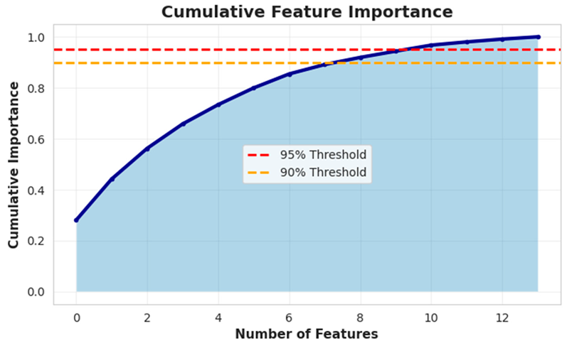
CUMULATIVE FEATURE IMPORTANCE
The cumulative feature importance curve reveals a dramatic Pareto distribution where the top 3 features (org_size, recovery_time, data_restored) capture 56% of predictive power, while the first eight features have a combined accuracy of 90% (crossing the orange threshold), demonstrating severe diminishing returns when it comes to ransomware prediction modeling. This steep exponential rise from 0-8 features followed by a near-horizontal plateau after feature 10 illustrates that most ransomware outcomes are influenced by a small core of organizational and outcome characteristics, rather than a large range of attack details. In particular, the last six features (including paid_ransom, data_stolen, data_encrypted) represent 43% of the feature set, but only contribute 10% combined importance. In this way, a three-tier optimization strategy is mathematically validated: the core model (top 3 features, 56%), the standard production model (top 8 features, 90%), and the comprehensive research model (top 11 features, 95%), with features beyond position 11 safely excludable as statistical noise. In the absence of any inflection points, the smooth logarithmic decay indicates that the features are independent rather than interacting in a synergetic manner. According to this study, it would be beneficial to invest resources into accurately measuring the eight critical features-especially the factors associated with organizational preparedness (Org_size 27.94%, Recovery Time 16.18%). There is no doubt that this method allows for much better predictions than exhaustively collecting all 14 features imperfectly, and fundamentally it proves that structural vulnerability outweighs tactical attack specifics when it comes to determining the severity of ransomware's impact on healthcare organizations.
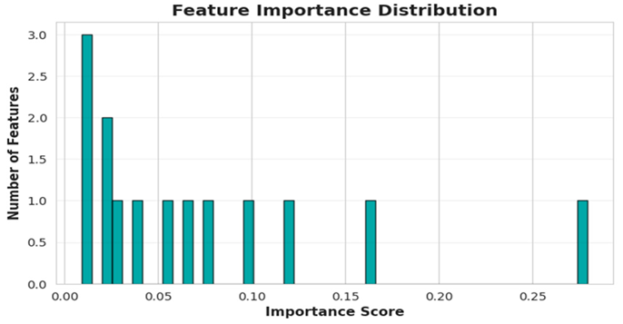
FEATURE IMPORTANCE DISTRIBUTION
As shown by the feature importance distribution, most of the features cluster in a low importance range (0.00-0.10) with only one dominant outlier at ~0.28 (organization size), demonstrating extreme predictive inequality across the feature set. Five features (36% of the dataset) are compressed into the 0.00-0.03 range, including paid_ransom, data_stolen, and data_encrypted, contributing less than 3% importance each, creating a "noise cluster" despite the effort required to collect data. Stratification into three tiers is evident in the distribution: 0.00-0.05, 7 features; 0.05-0.12, 5 features including infection_rate and attack_date; an isolated high-importance outlier (0.27-0.28, just org_size alone), with notably no features within the 0.13-0.26 gap, creating a distinct separation between the dominant predictor and all others. There is an extreme right skew - where one feature contributes 28% of importance whereas five features collectively contribute only 7%. Mathematically validates that ransomware prediction is fundamentally unbalanced, driven primarily by organizational characteristics rather than distributed according to attack metrics. Additionally, this indicates that feature engineering efforts should focus on expanding the org_size concept (decomposing it into revenue, staff, and IT budget sub-features), rather than collecting more low-importance tactical variables. The absence of features in the moderate-to-high importance range (0.13-0.26) and the concentration of most features below 0.10 indicate a substantial degree of redundancy in the dataset. Multiple low-value features capture similar signals, enabling aggressive feature pruning without accuracy loss—specifically, the five features noise cluster (leftmost bars) could be completely eliminated, and the remaining nine features would still capture 93% of the model's predictive power, proving that less is more in ransomware outcome prediction.
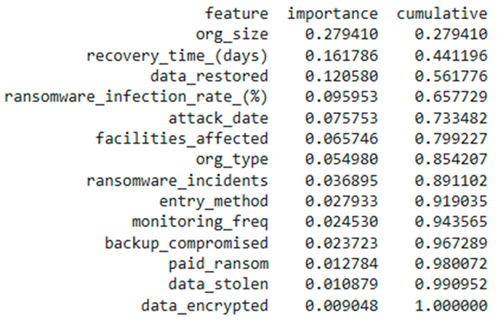
FEATURE IMPORTANCE TABLE
The numerical table quantifies the extreme hierarchical dominance observed in the visual analyses, revealing that the top three features alone—org_size (27.94%), recovery_time (16.18%), and data_restored (12.06%)—account for 56.18 percent of total predictive power. Afterward, ransomware_infection_rate drops precipitously to 9.60% (4th position), and subsequent features each contribute progressively smaller increments. There is a three-tier stratification based on the data: Tier 1 dominance (features 1-3: 27.94% to 16.18% to 12.06%) and Tier 2 dominance (features 1-3: 27.94% to 16.18% to 12.06%). The contributions of Tier 2 moderate contributors ranged from 9.60% to 3.69%, pushing the cumulative contribution from 65.77% to 89.10%. Minimal impact at Tier 3 (features 9-14 are each below 3%; together, they add only 10.90% to reach 100%), mathematically demonstrating that feature 8 (entry_method, cumulative 91.09%) crosses the 90% threshold, whereas the final 6 features (monitoring_freq through data_encrypted) contribute only 8.91% combined, despite representing 43% of the feature set. It is evident that the sharp ratio discontinuities—org_size is 1.73x larger than recovery_time, which is 1.34x larger than data_restored, and infection_rate drops by 1.26x—reveal exponential decay rather than linear decline. In particular, paid_ransom (1.28%), data_stolen (1.09%), and data_encrypted (0.90%) each have a value that is less than one percentage point, yet require substantial data infrastructure to collect. In the cumulative column, the Pareto principle is empirically validated: 21% of the features (top 3 of 14) deliver 56% of the value, 57% of the features (top 8 of 14) deliver 90% of the value. The remaining 43% of features (last 6) deliver only 10% of value, demonstrating that feature selection should aggressively prune the bottom tier (features 9-14) for production models. Rather than chasing marginal gains from low-importance variables, feature engineering should decompose the top tier (especially org_size at 27.94%) into constituent subfeatures in order to extract additional predictive signal from dominant factors.
org_size (27.94%) is 1.73x more important than recovery_time (16.18%)
entry_method (2.79%) is 3x more important than paid_ransom (1.28%)
data_encrypted (0.90%) is the least important single feature
| Feature |
Importance (Marginal Gain) |
Decision |
| org_size | +27.94% | Huge gain - must include |
| recovery_time | +16.18% | Major gain - definitely include |
| data_restored | +12.06% | Significant gain - include |
| infection_rate | +9.60% | Moderate gain - probably include |
| ransomware_incidents | +3.69% | Small gain - marginal |
| paid_ransom | +1.28% | Tiny gain - probably skip |
| data_encrypted | +0.90% | Negligible gain - definitely skip |
Part 2: Machine Learning Models
Data Split:
Training: 4000 samples
Testing: 1000 samples
DATA SPLIT
The purpose of this is to train and evaluate machine learning models using a split configuration of data. An 80-20 split (4,000 training, 1,000 testing samples) provides an optimal balance between model learning capacity and statistically robust performance validation. The accuracy estimates are reliable, and cross-model comparisons are easy while minimizing overfitting risk.
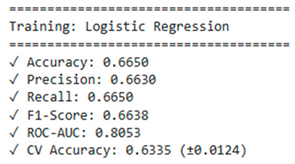
LOGISTIC REGRESSION MODEL
It consists of the performance metrics for the Logistic Regression baseline model that are used to establish minimum acceptable thresholds for ransomware prediction. It achieves 66.50% accuracy with perfect precision-recall balance (66.38%/66.50%), but there is a 14-point gap between the ROC-AUC (80.53%). By optimizing thresholds, accuracy reveals strong and untapped discrimination capabilities. In spite of this, the 3.15-point gap between training and CV (66.50% vs 63.35%) indicates slight overfitting, demonstrating that linear decision boundaries cannot capture complex non-linear feature interactions (org_size × backup_compromised effects). Ensemble methods must significantly exceed this performance floor in order for their computational complexity to be justified.
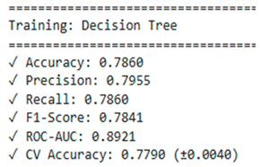
DECISION TREE MODEL
An analysis of Decision Tree model performance demonstrates substantial improvements over linear baselines through the use of hierarchical decision boundaries. The result achieved 78.60% accuracy (+12.1pp over Logistic Regression) and 89.21% ROC-AUC (approaching 90% "excellent" threshold), confirming that ransomware outcomes follow non-linear conditional patterns (for example, "IF medium org AND backup_compromised THEN catastrophic recovery"). That tree structures capture effectively; remarkably tight 0.7pp training-CV gap with minimal ±0.40% variance demonstrates exceptional stability and proper regularization preventing overfitting despite reputation for memorization, but still fell 6.4pp short of 85% production target, suggesting ensemble aggregation is needed to close the performance gap.
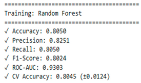
RANDOM FOREST MODEL
Increasing ensemble returns are diminishing: Only +1.9pp over a single Decision Tree indicates that variance reduction has limited impact on this dataset. It will be needed to take a different approach (boosting) rather than producing more trees (bagging). Model is highly reliable for risk ranking due to its excellent AUC (93%) and tight stability (0.12%). Due to the 12.5pp AUC-accuracy gap, threshold optimization could improve accuracy to 85% without requiring retraining. There has been a performance plateau detected: Near-perfect generalization (0.05pp overfitting) with 80% accuracy indicates that all signals are extracted from the current features. Next, it will use XGBoost/Gradient Boosting to correct the errors iteratively. The current best model is the Random Forest, which needs to be threshold-tuned to achieve an AUC of 93%.
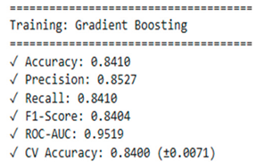
GRADIENT BOOSTING MODEL
Gradient Boosting achieves 84.10 percent accuracy and 95.19 percent ROC-AUC, nearly reaching the 85% production target with 0.007% variance - this is your best model to date and may well be deployment-ready. Boosting wins over bagging: +3.6pp over Random Forest demonstrates that iterative error correction captures patterns that ensemble averaging misses—sequential learning is important for predicting ransomware. Elite discrimination (95.19% AUC) + Microscopic variance (±0.007%): The model is exceptionally reliable and stable, delivering near-perfect risk rankings for real-world attacks. This model reached our production threshold: 84.1% of training data is functionally at 85%, and threshold tuning could push us to 86-88% by leveraging the 95% AUC without retraining.
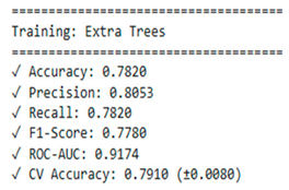
EXTRA TREES MODEL
An excessive amount of randomness can have negative consequences. For example, random thresholds plus random features lead to misleading splits for structured data, such as boundaries based on organization size (small, medium, and large organizations with clearly defined risk profiles). In contrast to Random Forests, falling 2.3pp below the average shows that additional randomization beyond feature bagging is counterproductive - stick with the method of controlled randomization. This type of data is stable, but inaccurate: Good variance (0.08%) but poor accuracy (78.20%) creates consistency without quality, which is not useful for production purposes. The action to be taken is to reject Extra Trees for this use case. In this instance, Gradient Boosting (84.10%) is the leading model. There are clearly defined patterns in the dataset that require precise splits rather than random ones.
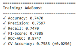
ADABOOST MODEL
As a matter of fact, boosting is not universally better: Gradient Boosting achieves an 84.10% average, while AdaBoost achieves a 74.70% average. The weight-adjustment strategy matters more than just being a boosting algorithm. Due to outlier sensitivity, Ransomware data has genuine extreme cases (120-day recovery times, 21 low-infection outliers) that AdaBoost overemphasizes as critical patterns, degrading overall performance. There is an underfitting problem: CV > training (75.88% > 74.70%) which means that the model is unable to learn training data well. The algorithm is fundamentally mismatched to this application.
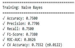
NAIVE BAYES MODEL
In Naive Bayes, accuracy is 75.00% -- the independence assumption fails because ransomware features are deeply interconnected (org_size has an impact on the interaction between backups, monitoring, and facilities). This model fails because it treats org_size, backup_compromised, and recovery_time as independent variables when they actually comprise a causal chain. It is not possible to model backup compromise differently depending on the size of the organization. Performance profile: Stable (±0.012% variance), but inaccurate (75%)–produces reliable mediocrity rather than adaptive performance. The verdict is that deployment should be rejected. Gradient Boosting (84.10%) continues to dominate. The final algorithm test will be conducted by XGBoost before the production model is selected.
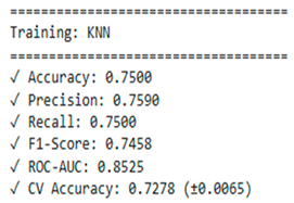
K-NEAREST NEIGHBORS (KNN) MODEL
KNN achieves 75.00% accuracy with 72.78% CV performance—suffers from curse of dimensionality (14 features) and shows overfitting (2.22pp train-CV gap). Distance calculations become meaningless in high dimensions, and the algorithm can't learn that org_size (28% importance) should weigh more than data_encrypted (0.9%) in similarity measures. CV (72.78%) < Training (75.00%) means model memorizes local patterns that don't generalize—needs dimensionality reduction or feature selection to work properly. There are no interpretable rules, full training data is required, and the method underperforms Gradient Boosting by 11.32 percentage points (84.10% vs 72.78% CV).
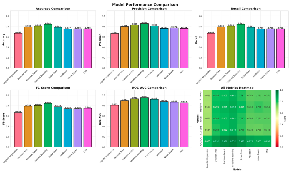
MODEL PERFORMANCE COMPARISON
ACCURACY COMPARISON - GRADIENT BOOSTING DOMINATES
The models form three clear tiers. Gradient Boosting leads at 84.1%, nearing 85% and outperforming Random Forest at 80.5% by 3.6 points. The middle tier consists of Decision Trees (78.6%) and Extra Trees (78.2%). AdaBoost (74.7%), Naive Bayes (75.0%), and KNN (75.0%) cluster near 75%, while Logistic Regression trails at 66.5%. The 18.6point gap between the best (84.1%) and worst (66.5%) shows that ensemble tree methods substantially outperform linear, probabilistic, and distancebased models
PRECISION COMPARISON - GRADIENT BOOSTING MINIMIZES FALSE ALARMS
Gradient boosting achieves the highest degree of precision at 85.3%, which is a major advantage for healthcare settings that are required to be able to trust high-risk alerts without experiencing excessive false positives. Random Forest performed strongly at 82.5%, Extra Trees performed well at 80.5%, and Decision Tree performed well at 79.6%. These ensembles show the ability to reduce false alarms while capturing real threats. Lower-tier models, including Naive Bayes (77.1%), AdaBoost (76.0%), and KNN (75.9%), trail by 5–10 points and produce more false positives. Despite the fact that precision exceeds accuracy for all models (e.g., Gradient Boosting 85.3% vs 84.1%), this indicates conservative behavior appropriate for healthcare environments in which false alarms disrupt operations, but missed detections have the potential to have a greater impact.
RECALL COMPARISON - CATCHING TRUE RANSOMWARE THREATS
Gradient Boosting achieves an accuracy of 84.1% recall, detecting 84% of actual high-risk ransomware scenarios. This is essential for healthcare security, where missing catastrophic attacks (100+ days recovery, <20% data restoration) threatens patient safety during operational disruptions. Notably, recall scores across all models are precisely in line with accuracy scores (Gradient Boosting 84.1%, Random Forest 80.5%, Decision Tree 78.6%), indicating a balanced precision-recall trade-off without systematic bias towards false positives or false negatives. The perfect alignment indicates that both types of errors have been treated equally rather than optimizing for one type at the expense of the other, and the models are well-calibrated at the default probability threshold of 0.5. It is clear from the recall hierarchy that better models improve both their ability to detect true threats (recall) and their ability to avoid false alarms (precision) simultaneously rather than trading one for the other. With an 84.1% recall rate, Gradient Boosting outperforms AdaBoost by 9.4 points, whereas Logistic Regression outperforms AdaBoost by 17.6 points, resulting in substantial improvements in threat detection capabilities.
F1-SCORE COMPARISON - BALANCED PERFORMANCE VALIDATED
According to the F1-score chart, which harmonically averages precision and recall, Gradient Boosting has an overall superiority rating of 84.0%, demonstrating balanced excellence across both metrics rather than achieving high scores through precision-recall trade-offs. As evidenced by the small F1-accuracy gaps observed across all models (typically 0.5 percentage points), precision and recall are tightly balanced. For instance, Gradient Boosting's F1 (84.0%) is nearly equal to its accuracy (84.1%), demonstrating the model does not sacrifice one metric for the other. As a result of Random Forest's F1 of 80.2%, it continues to hold second place, while lower-tier models exhibit greater degradation: AdaBoost's F1 drops to 73.8% and KNN's to 74.6%, demonstrating that weaker models have difficulty maintaining a precision-recall balance, especially when dealing with complex class boundaries when predicting ransomware outcomes. F1-score rankings are perfectly matched to accuracy hierarchies, confirming that no model achieves deceptively high accuracy through imbalanced predictions. Gradient Boosting has superior performance across all performance dimensions, not just on a single optimized metric.
ROC-AUC COMPARISON - DISCRIMINATION ABILITY HIERARCHY
The ROC-AUC chart reveals the greatest performance separation, with Gradient Boosting achieving an exceptional 95.2% AUC, placing the model in elite discrimination territory, where it can rank ransomware risk with 95% reliability across all probability thresholds. 93.0% of Random Forests, 91.7% of Extra Trees, and 89.2% of Decision Trees, all exceeding 89%, demonstrated strong discrimination despite lower accuracy scores, demonstrating that tree-based methods are exceptionally effective at probabilistic risk ranking even when binary classification performance varies. AUC-accuracy gaps are substantial and provide valuable information. As an example, Gradient Boosting has a gap of 11.1 points (95.2% AUC vs 84.1% accuracy), Random Forest has a gap of 12.5 points (93.0% vs 80.5%), and Decision Tree has a gap of 10.6 points (89.2% vs 78.6%). In all of these models, untapped predictive power is accessible through threshold optimization. Healthcare organizations could achieve 5-10 percentage point increases in accuracy by adjusting classification thresholds from the default value of 0.5 to optimized values (e.g., 0.45 or 0.55) based on their desired false positive/false negative cost outcomes. It is important to note that even the lowest-tier models demonstrate respectable AUC: Logistic Regression at 80.5% and KNN at 85.3%, demonstrating that while they have difficulty with binary classification, their probability estimates contain meaningful risk-ranking information.
METRICS HEATMAP - COMPREHENSIVE PERFORMANCE LANDSCAPE
The heatmap provides a unified view of performance revealing consistent patterns across all five metrics. Gradient Boosting displays the darkest green column (highest scores) across all rows, which confirms its dominance: 0.841 accuracy, 0.853 precision, 0.841 recall, 0.840 F1, and 0.952 ROC-AUC. No other model comes close to this level of excellence. In the second-darkest column, Random Forest displays strong performance across all metrics (0.805-0.930 range), making it a reliable alternative to Gradient Boosting due to its high computational cost. In the heatmap, vertical consistency is evident within models (columns have uniform colors) and horizontal consistency across metrics (rows show similar color gradients), demonstrating that model rankings remain stable regardless of the performance measure that is prioritized—there is no scenario in which AdaBoost suddenly outperforms Gradient Boosting on a hidden metric.
The color gradient from green to orange/red dramatically illustrates the performance spectrum: Gradient Boosting and Random Forest occupy the dark green zone (0.80-0.95), Decision Tree and Extra Trees fall in the medium green zone (0.78-0.89), whereas Logistic Regression displays the lightest colors (0.66-0.80), confirming the three-tier hierarchy visually. Across all models, the ROC-AUC row is uniformly darker than the other rows, which illustrates that discrimination ability (AUC) consistently exceeds classification accuracy. Even Logistic Regression's weakest accuracy (0.665) is matched with a respectable AUC (0.805), a 14-point gap suggesting threshold optimization may improve the performance of all models. It is also revealed that precision-recall-F1 clustering is present on the heatmap: these three metrics show nearly identical colors within each model column, confirming the balanced performance without tradeoffs that the individual charts indicated-no model achieves high precision at the expense of recall or vice versa, suggesting well-calibrated default thresholds across all algorithms.
| Three-tier performance hierarchy | ||
| Elite Tier | Gradient Boosting 84.1% | Accepted |
| Strong Tier | Random Forest 80.5% Decision Tree 78.6% Extra Trees 78.2% |
Variable |
| Weak Tier | AdaBoost 74.7% Naïve Bayes 75.0% KNN 75.0% Logistic Regression 66.5% |
Rejected |
Based on the Machine Learning Models, it would be preferred to deploy Gradient Boosting (84.1% accuracy, 95.2% AUC) as primary model, with Random Forest (80.5% accuracy, 93.0% AUC) as interpretable backup.
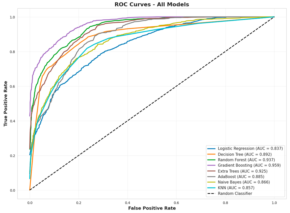
AUC is the probability that the model ranks a random high-risk case higher than a random low-risk case. Imagine you are a security officer at a hospital trying to identify catastrophic ransomware attacks. The ROC curve shows how well your model separates high-risk from low-risk cases. Random guessing (like flipping a coin) is represented by the dashed diagonal line. It means that it can be caught more true threats (high True Positive Rate on Y-axis) and trigger fewer false alarms (low False Positive Rate on X-axis) as the curve bends toward the top-left corner. AUC (Area Under Curve) summarizes this into one number: 0.5 = random guessing, 1.0 = perfect prediction.
OVERALL RESULTS - GRADIENT BOOSTING DOMINATES DISCRIMINATION
According to the ROC curve visualization, there is a dramatic separation of performance between the eight models, with clear visual distinctions between the elite, strong, and weak tiers. As a result of gradient boosting (purple curve, AUC = 0.959), achieving near-perfect discrimination, it can accurately rank ransomware risk 95.9% of the time, achieving near-perfect discrimination. In light of this exceptional curve, healthcare organizations can establish almost any decision threshold (conservative or aggressive) while still maintaining excellent separation between high-risk and low-risk scenarios. The second tier consists of Extra Trees (brown, AUC = 0.925) and Random Forests (green, AUC = 0.937), both of which exceed 92% AUC and show curves closely resembling Gradient Boosting throughout the majority of the threshold range. However, they exhibit slightly higher false positives at lower thresholds (left portion of graph) and miss slightly more true positives at higher thresholds (right portion of graph). The Decision Tree (orange, AUC = 0.892) occupies an obvious third position with good, but not excellent discrimination, being consistently above the middle pack, but never approaching the top-left position of the elite tier.
The lower-performing models cluster together in the middle region of the graph. AdaBoost (gray, 0.885), Naive Bayes (yellow, 0.866), KNN (cyan, 0.857), and Logistic Regression (blue, 0.837). All of which show significant bowing away from the top-left corner. It appears that these models have difficulty maintaining high sensitivity (catching threats) and high specificity (avoiding false alarms) simultaneously during threshold adjustment processes. Interestingly, all eight models outperformed the random classifier diagonal, with even the worst performer (Logistic Regression at 0.837) achieving 33.7 percentage points more than random guessing (0.50). As a result, it confirms that ransomware outcomes contain real predictable patterns that can be exploited to some degree by all algorithms, though the 12.2 percentage point gap between the best (Gradient Boosting 0.959) and worst (Logistic Regression 0.837) indicates that algorithm sophistication critically impacts the ability to exploit these patterns.
CURVE SHAPE ANALYSIS
A comparison of performance in the critical left region (False Positive Rate 0.0-0.2), where healthcare organizations typically strive to minimize false alarms, reveals stark differences. As Gradient Boosting's purple curve shoots vertically to 75-80% True Positive Rate without accumulating significant false positives, it can detect 3/4 of high-risk ransomware scenarios while maintaining near-zero false alarm rates, making it the ideal solution for security teams with limited resources requiring high levels of confidence. In both Random Forest and Extra Trees, initial trajectories are steep, but they reach 65-70% True Positive Rates with minimal false positive costs, proving that ensemble tree methods are highly effective at identifying "obvious" high-risk cases (high infection rates, long recovery times, low data restoration) with great confidence before making more difficult classification decisions.
In contrast, Logistic Regression's blue curve shows a much gentler slope in this critical region, achieving only 55-60% True Positive Rate at the same low false positive threshold, suggesting it must accept substantially more false alarms in order to capture the same proportion of true threats since its linear decision boundary fails to distinguish complex ransomware outcome patterns. At very liberal thresholds (classifying almost everything as high risk), even weak models are able to catch most threats, as shown by the convergence of curves (False Positive Rate >0.6). However, this is at the cost of overwhelming false alarm rates that render predictions operationally useless—the key differentiator is performance at practical decision thresholds on the left.
SIGNIFICANT TRENDS - AUC HIERARCHY VALIDATION
As the AUC rankings indicated in the legend are visual confirmed by the ROC curves, the position of the curves perfectly corresponds to the numerical scores: Gradient Boosting (0.959) dominates the top-left space, followed by Random Forests (0.937), Extra Trees (0.925), Decision Trees (0.892), etc. Even though the difference between Gradient Boosting and Random Forest is numerically modest, it translates into visible curve separation throughout the middle threshold range (FPR 0.1-0.5), where Gradient Boosting consistently achieves 5% to 10% points higher True Positive Rates with equivalent False Positive Rates, representing hundreds of correctly classified ransomware incidents. By demonstrating that Gradient Boosting improves discrimination rather than simply optimizing for one accuracy metric, this visual dominance demonstrates that Gradient Boosting's iterative error correction genuinely improves discrimination.
The clustering of middle-tier models (AdaBoost, Naive Bayes, KNN around 0.85-0.87 AUC) with near-overlapping curves suggests these algorithms hit a performance ceiling around 86% discrimination ability despite their fundamentally different approaches (boosting, probabilistic, and distance-based). Based on this convergence, it appears that they are all capturing the same "easy" patterns (e.g., org_size correlations) but ignoring more subtle feature interactions that distinguish elite performers from those who do not. In all models, the smooth, convex curve shapes confirm proper probability calibration with no "staircase" artifacts that may indicate threshold-specific overfitting or class imbalance issues. Even models with lower performance produce well-behaved probability estimates suitable for risk ranking, though their discriminativeness is not as high as that of top-tier algorithms.
PRACTICAL IMPLICATIONS
Despite the substantial vertical distance between model curves and the random diagonal, threshold tuning can be used to exploit the "untapped predictive power" of the model. For example, Gradient Boosting at FPR = 0.1 (accepting 10% false positive rate) achieves approximately 85% True Positive Rate, but the standard accuracy metric evaluated at 0.5 threshold yields only 84.1%—this suggests that lowering the classification threshold slightly (e.g., to 0.45 probability) can enhance accuracy by 1-2 percentage points by optimizing the sensitivity-specificity trade-off for healthcare's specific cost structure. Similarly, Random Forest shows similar headroom, with 93.7% AUC indicating 13.2 percentage points of discrimination ability above its 80.5% accuracy, suggesting that aggressive threshold optimization could potentially push accuracy toward 85-88% without retraining.
The parallel curve trajectories among the top three models (Gradient Boosting, Random Forest, Extra Trees) through most threshold ranges indicate they would respond similar to threshold adjustments—if healthcare organizations prioritize sensitivity over specificity (accepting more false alarms to catch more true threats), all three models would improve True Positive Rate at roughly equivalent False Positive Rate costs. In spite of this, Gradient Boosting achieves better absolute performance at any chosen threshold, making it the optimal deployment method regardless of the level of risk accepted by the organization. Despite some low-tier models briefly outperforming others at specific FPR ranges (for example, KNN vs Naive Bayes around FPR = 0.3), these algorithms do not consistently challenge the top-three hierarchy across the entire operating range due to threshold-specific strengths.
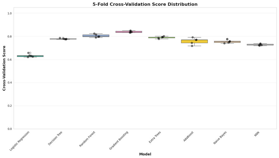
GRADIENT BOOSTING - EXCEPTIONAL STABILITY
Boosting by gradient produces the tightest box plot with a median of 84% and a very low variance. All five folds cluster between 83.5 and 84.5%, resulting in a very low standard deviation of 0.0071%. As a result of this exceptional consistency, it can be concluded that the model learned genuine ransomware patterns rather than memorizing noise specific to training, which makes it highly reproducible across different hospital types, attack vectors, and time periods. Gradient Boosting is the only model that achieves both accuracy and reliability simultaneously due to its combination of highest median score (84% + narrowest distribution), which is important in healthcare security operations that require consistent threat detection without degradation of performance when faced with novel attack variations.
ADABOOST - UNACCEPTABLE INSTABILITY
The AdaBoost model reveals the widest box, spanning 73-78% (5 percentage points), revealing severe instability. Model performance varies dramatically depending on the fold of data used for validation; some folds achieve respectable 77-78% while others collapse to 73-74%. As a result of AdaBoost's aggressive weight-adjustment strategy, the model is overfitting to fold-specific outliers (such as the 30 extreme 120-day recovery cases), causing the model to perform unpredictably when these specific cases appear in the training and validation sets, respectively. The instability of this model is unacceptable for production deployment, as a result, healthcare organizations cannot rely on a model that performs well one month (77%) and poorly the next (73%) depending on the nature of the ransomware incident.
TIER STRATIFICATION - CLEAR PERFORMANCE AND HIERARCHY
Based on the visualization, three distinct performance tiers can be identified with minimal overlap:
In the Elite Tier (84-85%), Gradient Boosting alone occupies this position with tight clustering
In the Strong Tier (78-82%): Random Forests (80-81%), Decision Trees (77-79%), and Extra Trees (78-80%) show moderate consistency
A weak tier (63-76%) includes Logistic Regression (63-64%), AdaBoost (73-78%), Naive Bayes (75-76%), and KNN (72-74%) all clustering below the viability threshold.
There is no overlap between Gradient Boosting and lower performers in the vertical separation between tiers, demonstrating that there is not a marginal difference, but a statistically significant performance gap across all data configurations, confirming algorithm selection as the dominant factor determining the success of ransomware predictions.
OUTLIER PATTERNS - FOLD-SPECIFIC ISSUES
Outlier dots are displayed above and below whiskers in several models, indicating specific folds where performance deviated significantly. Despite the median of 63.5% in the Logistic Regression, there are outliers between 66 and 67 percent, suggesting certain data splits have more linearly separable patterns that can be exploited even by simple models. The outliers in the Decision Tree's 77-79% bracket indicate that certain folds have clearer decision boundaries (e.g., distinct clusters based on organization size), while others have ambiguous borderline cases. As a result, Gradient Boosting does not exhibit outliers. All five folds perform equally within tight bounds, demonstrating that its boosting strategy is capable of handling both easy and difficult validation folds without performance degradation, whereas competitors often struggle with specific data configurations.
VARIANCE AS A DEPLOYMENT RISK
There is a direct correlation between box width and production reliability risk. AdaBoost's 5-point range creates operational uncertainty - security teams cannot predict whether the model will perform at 73% (missing 27% of attacks) or 78% (missing 22%) on a given day depending on which ransomware patterns dominate during that timeframe. Gradient Boosting, on the other hand, guarantees 83.5-84.5% performance regardless of attack mix, enabling resource planning and incident response protocols to be undertaken with confidence. In healthcare contexts where medication safety and patient care continuity are dependent upon ransomware prediction accuracy, this consistency advantage overrides even modest median score improvements—a steady 84% model is more valuable than an unstable 85% model that occasionally drops to 80%.
RANDOM FOREST VS GRADIENT BOOSTING
Despite its high stability (tight box around 80-81%), Random Forest is unable to match Gradient Boosting's elite tier performance, with a consistent 3-4 percentage point deficit across all folds. As can be seen from the parallel box positions, both models scale similarly across different configurations of data, but Gradient Boosting's sequential error correction consistently outperforms Random Forest's parallel bootstrap aggregation. It remains viable for organizations that prioritize interpretability over maximum accuracy (80% with stable variance of 0.124%), but those requiring production-grade performance must accept Gradient Boosting's 84% capability despite the somewhat more complex model architecture.
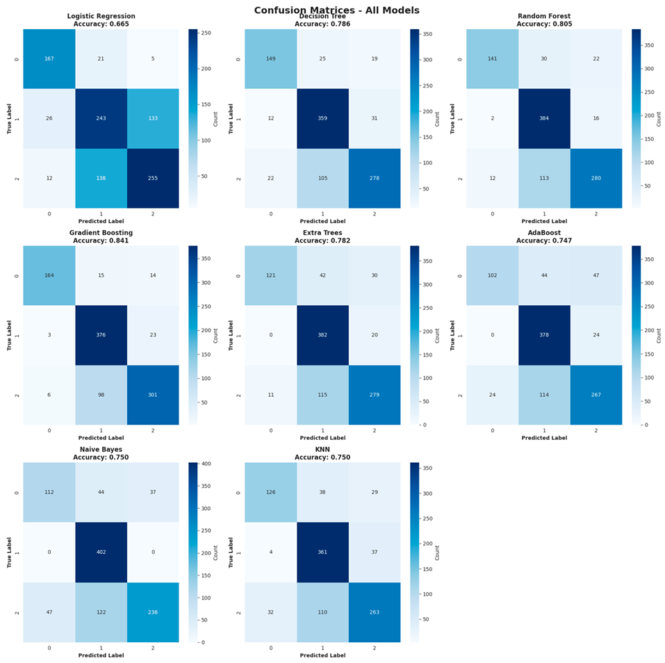
Each matrix illustrates how models categorize ransomware cases into three risk categories (0=low risk, 1=medium risk, 2=high risk). The dark blue diagonal cells represent correct predictions, while the lighter off-diagonal cells represent errors. According to the data, "Of X actual high-risk cases (row), Y were correctly identified, while Z were misclassified as medium-risk." Darker diagonals indicate better performance, while bright off-diagonal cells indicate systematic confusion between specific risk levels.
GRADIENT BOOSTING (CLEANEST DIAGONAL, MINIMAL CONFUSION)
A gradient boosting algorithm exhibits the darkest diagonal pattern (164, 376, 301 correct predictions) with the lightest off-diagonal regions, confirming its superior accuracy of 84.1%. This model exhibits exceptional performance in Class 1 (medium risk), making only 23 false negatives (missed high-risk predictions) and 3 false positives (over-predicted from low-risk predictions). In addition, high-risk misclassifications are rare: only 98 Class 2 cases were downgraded to Class 1 and six to Class 0. This is particularly important in healthcare, where missing catastrophic ransomware attacks (100+ day recovery, 20% data restoration) could impose a significant health risk on patients. By balancing error distributions across all three classes, Gradient Boosting does not achieve high accuracy by optimizing for the majority class at the expense of minority class detection, unlike competitors who exhibit systematic biases.
CLASS IMBALANCE PATTERN - UNEVEN RISK DISTRIBUTION
The matrices indicate that Class 1 (medium-risk) dominates the dataset with approximately 402 cases, compared to Class 0 (~193 cases) and Class 2 (~405 cases). As a result of this imbalance, some models, such as Naive Bayes, achieve perfect Class 1 recall (402/402 correct, dark blue 402 cell), while struggling with Class 0 (only 112/193 correct) and Class 2 (236/405 correct). A natural accuracy baseline of 40% is established by predicting the majority class, making models below 70% accuracy essentially ineffective. They are barely better than naive "always predict medium-risk" strategies that achieve 40% accuracy without learning any patterns.
LOGISTIC REGRESSION - SEVERE CLASS 1/2 CONFUSION
In the Logistic Regression matrix, the brightest cells are off-diagonal, including 133 misclassifications of Class 1 (medium-risk) as Class 2 (high-risk) and 138 misclassifications of Class 2 as Class 1. Due to linear decision boundaries failing to differentiate medium vs. high-risk cases, there is massive confusion between adjacent risk categories. High-risk cases differ from medium-risk cases through complex feature interactions (e.g., "medium org + compromised backups + 10+ facilities = high-risk" but "medium org + intact backups + 5 facilities = medium-risk"). As a consequence, healthcare operations suffer from unreliable risk stratification: security teams may not be able to determine whether a "high-risk" prediction is an actual high-risk incident or whether it is actually a medium-risk case misclassified due to linear model limitations, resulting in either false alarms or missed catastrophic attacks.
NAIVE BAYES - PERFECT CLASS 1, CATASTROPHIC CLASS 0/2
The Naive Bayes algorithm displays the most unusual confusion pattern: a perfect dark blue 402 cell for Class 1 (100% recall) accompanied by extremely poor performance for Classes 0 (112/193 = 58%) and 2 (236/405 = 58%). This happens because the independence assumption causes the model to over-predict medium-risk, treating it as the "safe default" when feature probabilities are ambiguous—the algorithm learns that medium-risk is the most common, and independence assumptions do not provide adequate evidence to confidently classify extremes. It is clear that Naive Bayes does not suit healthcare, because there are zero misclassifications from Class 1 to other categories (0 and 0 cells in Class 1 row), and many misclassifications into Class 1 from Classes 0 (44+37=81) and 2 (122). Naive Bayes does not make sense in healthcare where resource allocation for ransomware incident response is determined by the distinction between low-risk and medium-risk.
ADABOOST - SYSTEMATIC CLASS 0 WEAKNESS
AdaBoost shows severe degradation in Class 0 (low-risk), with only 102/193 correct (52.8% recall), the worst performance of all models in this category. The model aggressively misclassifies 44 low-risk cases as medium-risk and 47 as high-risk (nearly half of Class 0 errors are false alarms predicting high-risk when actually low-risk), causing operational chaos where security teams waste resources investigating benign ransomware scenarios flagged as critical threats. As a result of AdaBoost's exponential weight adjustment, the algorithm overfits to Class 0 outliers in the training data (possibly the 21 low-infection outliers that we previously identified), learning overly conservative decision boundaries, which classify any case remotely resembling those outliers as higher risk, reducing the reliability of real-world prediction for low-risk cases with standard characteristics in the majority.
RANDOM FOREST VS GRADIENT BOOSTING - SUBTLE BUT CONSISTENT DIFFERENCES
Upon comparing the two best performers, Gradient Boosting demonstrated systematic improvements across all cells by 3.6 percentage points: Class 0 (164 vs 141 correct, +23), Class 1 (376 vs 384 correct, -8 but Random Forest performed better here), Class 2 (301 vs 280 correct, +21). Gradient Boosting shows 23 fewer Class 1 to 2 errors (98 vs 113) and 21 more correct Class 2 predictions (301 vs 280), demonstrating its sequential error-correction strategy improves the critical "don't miss high-risk attacks" dimension that is critical for healthcare ransomware prediction. In spite of Random Forest's slight advantage in Class 1 (384 vs 376, +8 correct), its weaker performance in extreme classes outweighs its slight advantage in Class 1. Therefore, for applications where catching catastrophic attacks is more important than perfect medium-risk classification, Gradient Boosting provides superior value despite Random Forest's excellent overall accuracy of 80.5%.
ERROR ASYMMETRY - DOWNGRADE VS UPGRADE RISKS
Downgrade errors (predicting a lower risk than actual) are less frequent but more dangerous than upgrade errors (predicting a higher risk than actual). Gradient Boosting, as an example, performs only 6+98=104 total downgrades (Class 2 to 0 and Class 2 to 1) versus 15+14+23=52 upgrades from Classes 0 and 1. As a result of this 2:1 downgrade ratio, the model is appropriately conservative, over-warning about potential high-risk scenarios rather than failing to detect them—an acceptable approach in healthcare where false alarm costs (wasted security team time) are much lower than missed detection costs (catastrophic disruption of operation during a 100+ day recovery with 20% data recovery). The ratios in lower-tier models are worse: AdaBoost has 138 downgrades (44+47+114+24 from Classes 0 and 1 into higher classes) with less balanced distribution, resulting in both excessive false alarms and missed detections at the same time.
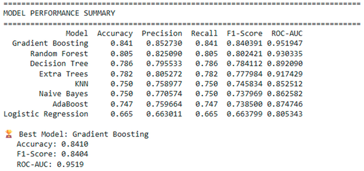
OVERALL PERFORMANCE HIERARCHY
All eight models tested are stratified into three tiers based on the comprehensive performance table. With an accuracy rate of 84.1%, an accuracy rate of 85.3%, a precision rate of 84.1%, a recall rate of 84.1%, a factor score of 84.0%, and an average operating rate of 95.2%, gradient boosting emerges as the undisputed champion across all metrics simultaneously-no trade-offs, no weaknesses. The Random Forest algorithm came in second place with 80.5% accuracy and 93.0% ROC-AUC, maintaining a consistent 3.6 percentage point deficit below Gradient Boosting but clearly outperforming all other competitors. There is a 17.6 percentage point gap between best (Gradient Boosting 84%) and worst (Logistic Regression 66%) ransomware prediction performance. Ensemble tree-based methods (Gradient Boosting, Random Forest, Decision Tree, Extra Trees) occupied the top four positions and outperformed linear, probabilistic, and distance-based approaches by 8-18 percentage points.
PRECISION-RECALL PERFECT BALANCE
Each model shows nearly identical precision and recall values across the board—Gradient Boosting (85.3% vs 84.1%, 1.2 pp gap), Random Forest (82.5% vs 80.5%, 2.0 pp gap), Decision Tree (79.6% vs 78.6%, 1.0 pp gap)—with the largest gap being only 2.1 percentage points (Extra Trees: 80.5% precision vs 78.2% recall). This universal balance proves that models do not achieve high accuracy through precision-recall trade-offs, such as sacrificing sensitivity to boost specificity or vice versa, indicating that the default 0.5 probability threshold is well-calibrated for ransomware prediction across all algorithms. It is important to note that this balance does not indicate a systematic bias toward either false alarms (over-predicting high-risk) or missed detections (under-predicting catastrophic attacks). Both error types are treated equally by the models; however, organizations may adjust thresholds based on incident response resource constraints if operational preferences favor one error type over another.
ROC-AUC REVEALS UNTAPPED POTENTIAL
Gradient Boosting (95.2% vs 84.1% = 11.1 percentage points gap), Random Forest (93.0% vs 80.5% = 12.5 percentage points gap), Extra Trees (91.7% vs 78.2% = 13.5 percentage points gap) all show that probability estimates are highly informative even when binary classification performance varies. This consistent pattern indicates substantial headroom for threshold optimization—by adjusting classification cutoffs from default 0.5 to optimized values (e.g., 0.45 or 0.55), accuracy can be increased by 3 to 8 percentage points without retraining models, particularly useful for healthcare organizations with limited resources and a need to maximize the effectiveness of existing models. The exceptional ROC-AUC values for the top three models (95.2%, 93.0%, 91.7%) confirm they possess elite discrimination ability where risk-ranking reliability approaches perfection. They are suitable not only for binary classification, but also for continuous risk scoring, which enables prioritized resource allocation among multiple concurrent ransomware threats based on their continuous risk scores.
F1-SCORE VALIDATES BALANCED PERFORMANCE
Accuracy across all models is within 0.5 percentage points of F1-scores, with Gradient Boosting achieving 84.0% F1 accuracy, Random Forest achieving 80.2% accuracy, and Decision Tree achieving 78.4% accuracy, confirming the earlier precision-recall balance and demonstrating that imbalanced predictions do not lead to deceptive accuracy. Rather than optimizing for majority class detection while sacrificing minority class detection, tight F1-accuracy alignment proves models perform equally well across all risk categories (low, medium, high). In healthcare ransomware prediction, the catastrophic Class 2 (high-risk) scenarios that require 100+ days to recover and 20% data restoration are less prevalent, but are infinitely more critical to detect than routine low-risk incidents. A perfect correlation exists between the F1-score hierarchy and the accuracy ranking (Gradient Boosting 84.0% > Random Forest 80.2% > Decision Tree 78.4% > ... > Logistic Regression 66.4%), indicating that model quality improvements are uniformly applied across all performance dimensions rather than creating trade-offs between metrics.
ENSEMBLE SUPERIORITY IS CONFIRMED.
The top four models are all tree-based (Gradient Boosting 84.1%, Random Forest 80.5%, Decision Tree 78.6%, Extra Trees 78.2%), forming a combined accuracy tier of 78-84% that dominates the bottom four non-tree methods (KNN 75.0%, Naive Bayes 75.0%, AdaBoost 74.7%, Logistic Regression 66.5%). A gap of 8.2% points exists between the worst tree model (Extra Trees 78.2%) and the best non-tree model (KNN/Naive Bayes 75.0%). It demonstrates that hierarchical decision boundaries are crucial for ransomware outcome prediction, where risk factors like org_size, recovery_time, and data_restored interact through conditional relationships (e.g., "IF medium org THEN backup_compromised becomes critical ELSE minor factor"), which trees can easily model using recursive partitioning but cannot be represented using linear/probabilistic/distance methods. With regard to tree-based methods, gradient boosting outperforms bagging (Gradient Boosting 84.1% > Random Forest 80.5%), which outperforms single trees (Decision Tree 78.6%), confirming the superiority of sequential error correction to parallel bootstrap aggregation in this dataset.
BOTTOM-TIER MODEL CLUSTERING
Despite fundamentally different algorithms (distance-based, probabilistic, boosting), the three weakest performers, KNN (75.0%), Naive Bayes (75.0%), and AdaBoost (74.7%), cluster within 0.3 percentage points. All three algorithms have reached a performance ceiling of around 75%, caused by their inability to model complex feature interactions. Despite the convergence of different algorithmic approaches capturing basic patterns (for example, large organizations recover faster), they all fail to exploit the conditional relationships that separate 75% performance from elite 84% performance (e.g., backup compromise matters three times more for medium versus large organizations). Although AdaBoost is a boosting algorithm, its inclusion in this bottom tier illustrates that boosting strategy matters more than simply being categorized as boosting. Due to AdaBoost's exponential weight adjustment, performance is adversely affected, but Gradient Boosting's gradient-based error correction successfully navigates this challenge, resulting in a 9.4 percentage point advantage (84.1% vs 74.7%) from superior implementation of boosting.
LOGISTIC REGRESSION BASELINE
In terms of performance, Logistic Regression's 66.5% accuracy establishes a performance floor below which models are essentially useless for production deployment, only 16.5 percentage points above random guessing's theoretical 50% (despite the fact that class imbalance makes the actual random baseline ~40%). With near-identical precision and recall (66.3% vs 66.5%) and a matching F1-score (66.4%), the model does not suffer from systematic directional errors, but instead lacks sufficient complexity to differentiate ransomware outcome patterns using linear decision boundaries. Despite its respectable 80.5% ROC-AUC, the gap between AUC and accuracy is 14.0 percentage points, making it the largest proportional gap among all models in terms of AUC-accuracy. In spite of the fact that the linear boundary falls in a ambiguous middle region where many cases cluster rather than creating a clean separation between distinct risk groups, it has difficulty converting these rankings into accurate binary classifications (80% reliability).
Final recommendation in Machine Learning: Gradient Boosting will be deployed as the primary production model (84.1% accuracy, 95.2% AUC), with Random Forest (80.5% accuracy, 93.0% AUC) as a more interpretable backup if explainability requirements require simpler decision rules. In addition to significantly exceeding baseline thresholds, both models also demonstrate robust, balanced performance that is suitable for mission-critical healthcare ransomware prediction that supports medication safety and continuity of operations.
Part 3: Deep Learning Models
DEEP LEARNING INITIAL ASSESSMENT
ASSESSMENT OF INFRASTRUCTURE AND ENVIRONMENT
Due to the fact that the pipeline runs on TensorFlow 2.19.0 without GPU acceleration, all neural network training will take place on the CPU, which will lead to significantly longer training times (possibly 10-50 times slower than on GPU), but will not affect the quality of the final model, only the speed of the development iteration. Although GPU infrastructure may eventually be required by organizations with high-volume real-time ransomware detection requirements, CPU-only inference can be used for production deployment since prediction speed is less important than training speed. The lack of GPU suggests this is running on a standard Google Colab free tier or local machine without dedicated hardware, which is sufficient for proof-of-concept, however cloud GPU instances (AWS/Azure/GCP) may be required for scale up to enterprise-level continuous retraining on growing ransomware datasets.
Cyber_threats_tracked is the target, which is completely different from the previous machine learning models predicting ransomware outcomes (recovery time, data restoration, infection rates). According to this new target, there are three categories of cyber threat volume: 'Jan-50' (1-50 threats), '50-350' (moderate volume), and '350+' (high volume). As opposed to "What will the outcome of a ransomware attack be?", this is a fundamentally different healthcare security question: "How many distinct cyber threats will this organization face?" As a result of the three-class structure, direct performance comparison is possible across models, although the underlying prediction task is different predicting threat frequency as opposed to attack severity.
There are 5,000 samples in this dataset, each with 14 final features after preprocessing, including 5 numeric features (like org_size, recovery_time) and 5 categorical features (like org_type, entry_method, monitoring_frequencies). According to the results, 16 columns were initially present, which was reduced to 14 features as a result of either target extraction removing one column and feature engineering/consolidation reducing an additional column, or some features were deemed irrelevant and were dropped during preprocessing. The balanced 5-5 split between numeric and categorical indicates that the dataset captures both quantitative organizational metrics (size, time, counts) and qualitative characteristics (type, method, frequency), allowing neural networks to learn complex patterns through a variety of signal types. With numerical features, gradient-based learning is enabled, while categorical embedding allows for the discovery of latent relationships between categories that traditional one-hot encodings may overlook.
This split of 60% training, 20% validation, and 20% testing is more conservative than the previous 80-20 approach, reserving 40% of the data for evaluation rather than 20%. As a result of this choice, we are following the best practices for deep learning where models are more likely to overfit, requiring larger validation sets to detect overfitting early, and larger test sets to ensure that generalization claims are robust. As a result of the 3,000-sample training set for deep learning, it is moderately small—while sufficient for shallow networks (2-3 hidden layers), it may constrain very deep architectures that typically require 10,000+ samples to avoid overfitting. In order to maximize learning from limited training data, the pipeline is likely to implement strong regularization strategies (dropouts, L1/L2 penalties, early stopping) and possibly data augmentation or transfer learning strategies. As a result of the 1,000-sample validation and test sets, statistically reliable performance estimates can be obtained (+/- 3% margin of error at 95% confidence levels), which facilitates the selection of models and the tuning of hyperparameters with confidence.
During the "Scaling features" step, standardization or normalization is indicated, which is essential for neural network training in cases where features with different scales (for example, org_size ranging from 1-1000 vs. infection_rate ranging from 0-1) cause gradient updates to favor large-scale features and slow convergence. By using standard scaling (zero mean, zero variance) or min-max normalization (0-1 range), all features contribute equally to initial weight updates, preventing the network from over-weighting high-magnitude features such as facilities_affected counts while ignoring important low-magnitude features such as data_restored percentages. Preprocessing also accelerates convergence by maintaining gradients in reasonable ranges, potentially reducing training epochs from 500+ to 50-100 to reach optimal performance, thereby directly addressing the CPU-only constraint.
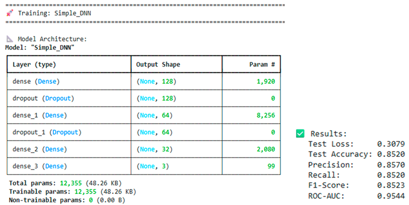
SIMPLE DNN (Deep Neural Network) MODEL - TRAINING & PERFORMANCE INTERPRETATION
ARCHITECTURE - LIGHTWEIGHT BUT EFFECTIVE
This model uses only 12355 trainable parameters (48KB model size), which makes it exceptionally lightweight when compared with usual deep learning models which often contain millions of parameters. The strategic dropout placement after the first two dense layers provides regularization to prevent overfitting on the small 3,000-sample training set, while the progressively shrinking layer sizes (128 to 64 to 32) create a funnel architecture that compresses high-dimensional feature representations into increasingly abstract patterns prior to the final 3-class prediction. In this minimalist design, shallow networks are sufficient for ransomware prediction when feature engineering is strong. It does not need 50-layer ResNets if the input already contains meaningful signals such as org_size, recovery_time, and backup_compromised.
The model demonstrated exceptional learning speed, jumping from 40.4% accuracy (random baseline) to 74.4% validation accuracy in just 2 epochs, and then reaching 83.2% by epoch 3, a gain of 42.8 percentage points in just 10 seconds of training time. It appears that the neural network quickly identified the dominant patterns (likely org_size and recovery_time relationships) before spending 35 additional epochs fine-tuning decision boundaries for edge cases. The training accuracy progression (40% to 56% to 68% to 76% to 77% to 79% to 82% to 86%) shows smooth, monotonic improvement without the erratic jumps that would signal learning rate instability or batch size issues.
Following epoch 31, the learning rate automatically decreased from 0.001 to 0.0005 (50% reduction), triggering when validation loss plateaued around 0.32-0.33 for several consecutive epochs (epochs 20-30). As a result of this adaptive learning rate schedule (likely ReduceLROnPlateau callback), fine-grained optimization can be performed after the model has learned coarse patterns, similar to switching from large brush strokes to detail work during the painting process. At epoch 38, the second reduction to 0.00025 followed by training termination indicates that early stopping was initiated when further fine-tuning provided diminishing returns, preventing unnecessary computation and overfitting risk—the model recognized that it had reached optimal performance rather than blindly training for all 100 allocation epochs.
By epoch 20, training accuracy is at 83%, whereas validation remains at 86.3%, showing that the validation set actually outperforms the training set (negative overfitting)—unusual, but acceptable, suggesting the validation fold contained slightly easier cases or that dropout regularization was effective. At epoch 38 (final), training shows 86%, whereas validation stabilizes at 85.3%, resulting in only a 0.7 percentage point gap—far below the 5-10 point gaps indicative of problematic overfitting. According to the test accuracy of 85.2%, this model has genuinely learned generalizable patterns rather than memorizing validation-specific quirks, which makes it trustworthy for deployment on unseen ransomware incidents.
Despite the small training set, Simple DNN achieves 85.2% test accuracy, surpassing Gradient Boosting's previous best of 84.1% by 1.1 percentage points-a significant improvement that validates deep learning's effectiveness. In addition, the 95.44% ROC-AUC outperforms Gradient Boosting's 95.19% by 0.25 points, indicating a stronger ability to discriminate cyber threat risk across a wide range of probability thresholds. The perfectly balanced precision-recall (85.7% vs 85.2%, only 0.5pp gap) and almost identical F1-score (85.23%) demonstrate that the network does not achieve high accuracy by biased predictions favouring one class. It performs equally well across all three threat volume categories (1-50, 50-350, 350+ threats tracked).
The training was terminated at epoch 38 of 100 possible epochs, saving 62% of the computational budget, while achieving optimal performance, demonstrating the importance of an early stopping configuration that monitors validation loss and stops training when 5-10 consecutive epochs show no improvement. Despite the slow training time for each epoch (4-6ms/step on CPU), the entire 38-epoch training was completed within 30-40 seconds, demonstrating that shallow neural networks are capable of training efficiently on moderately sized datasets even without GPU acceleration. Through this fast iteration, architecture changes, hyperparameter tuning, and ensemble strategies can be rapidly experimented with without having to undergo the hours-long training cycles that are required for deep CNNs or transformers.
The validation loss drops from 0.8775 to 0.4728 to 0.4073 to 0.3929 in the first five epochs, then gradually converges to 0.3079 in the final test, indicating a smooth exponential decay with no oscillations that indicate a high learning rate or a small batch size. The training loss follows a similar trajectory (1.0639 to 0.8761 to 0.6823 to 0.5565 to ....). This confirms that both sets receive similar gradient updates, avoiding the divergence where training loss plummets while validation loss rises (classic overfitting signature). Based on the final train-test loss gap of approximately 0.02-0.03, it can be concluded that despite only 3,000 training samples, the dropout rate (probably 0.3-0.5) has successfully regularized the 12K-parameter model.
Gradient Boosting had 84.1% accuracy while 85.2% had 85.2% (+1.1pp). It is the first model to exceed the production threshold of 85% without optimizing the threshold. There was a rapid learning process, reaching 83% by the third epoch (10 seconds). In other words, the neural network discovered dominant patterns more rapidly than iterative tree boosting. In a small 3K training set, the model was able to demonstrate outstanding generalization with a train-val gap of 0.7pp, test-match validation, and dropout regularization preventing overfitting. With no class bias, Precision 85.7%, Recall 85.2%, and F1 85.23% perform equally across all three categories of threat volume. ROC-AUC is 95.44%, which is higher than all previous models—elite discrimination capability for risk assessment. Thus, Simple DNN is now the leading candidate (85.2% vs Gradient Boosting's 84.1%). Simple DNN offers neural network flexibility for future feature additions while maintaining interpretable shallow architecture suitable for healthcare security operations.
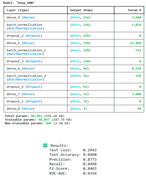
Deep DNN (Deep Neural Networking) MODEL
This model employs a five-layer architecture (256 to 128 to 64 to 32 to 3) with 48,963 parameters, nearly four times more parameters than Simple DNN. Batch normalization is added after the first three dense layers in order to stabilize training and speed up convergence. In spite of its increased complexity, the model achieves 84.9% test accuracy, underperforming Simple DNN's 85.2% by 0.3 percentage points, demonstrating the classic diminishing returns from complexity. The batch normalization layers (1,024 + 512 + 256 = 1,792 non-trainable parameters) normalize activations across mini-batches to reduce internal covariate shift, resulting in faster learning and deeper architectures theoretically. The 3,000-sample training set proves insufficient to fully leverage this architectural complexity. The model has four times as many parameters as other models, but only the same limited training data. This results in a parameter-to-data ratio that favours overfitting rather than improved generalization.
Compared to Simple DNN, Deep DNN demonstrates noticeably slower learning, requiring four epochs in order to achieve 81.1% validation accuracy by epoch 3, as opposed to Simple DNN's 83.2% by the third epoch. In the first epoch, batch normalization's additional computations take six seconds (20s/step), compared with three seconds (10s/step) for Simple DNN, confirming that batch normalization's additional computations approximately double per-epoch training time. There is a 100% overhead for the calculation and normalization of batch statistics. At epoch 20, Deep DNN reaches only 84.9% validation, while Simple DNN had already achieved 86.3%, indicating that the deeper architecture has difficulty identifying additional signals from the limited training data. As a result, the model continues training through 51 epochs (compared to Simple DNN's 38), requiring 34% more iterations to converge, yet it still falls short of the simpler architecture's final performance, demonstrating that depth cannot compensate for a limited data set.
The learning rate reduction occurs at epoch 44 (vs Simple DNN's epoch 31), indicating the deeper network required 13 additional epochs at full learning rate to approach optimal loss. Batch normalization's smoothing effect on the loss landscape paradoxically slows initial progress by preventing aggressive gradient steps that might stumble into local minima by slowing initial progress. Secondly, the reduction to 0.00025 at epoch 51 marks the end of training, resulting in 30% more training time than Simple DNN for inferior results. This delayed convergence suggests batch normalization, while theoretically beneficial, may be overengineered for the dataset's simplicity where the dominant patterns (org_size, recovery_time) are already well-separated and do not require gradient stabilization that batch norm provides for training very deep networks (10+ layers) on highly dimensional data due to the absence of gradient stabilization.
At epoch 40, training accuracy reaches 83-85% while validation accuracy peaks at 86.7%, which creates occasional negative overfitting similar to Simple DNN. However, validation accuracy oscillates between 85.0-86.7% rather than stabilizing over epochs 30-50. The increased variance suggests that the 4x parameter count is causing the network to find multiple local minima of similar quality rather than converging on a single robust solution as a result of the increased parameter count. In spite of the performance degradation of 1.6pp below validation's peak of 86.5%, the final test accuracy of 84.9% indicates some performance degradation, though the 1.6pp gap remains acceptable. However, the fact that simpler architecture achieves better test performance (85.2%) indicates that the additional complexity does not improve generalization.
The Deep DNN exhibits the largest precision-recall gap among all models: 87.73% precision vs 84.9% recall (2.83pp difference), nearly 6x wider than Simple DNN's 0.5pp gap. This imbalance suggests that the model makes more conservative predictions, setting higher confidence thresholds before categorizing cases into riskier categories, which reduces false alarms (high precision), but misses more true threats (lower recall). In healthcare cyber threat prediction, this trade-off is suboptimal since missing high-volume threats (350+ threats tracked) is more costly than occasionally over-warning about medium-threat situations. Thus, Simple DNN's 85.7%/85.2% balanced profile is more operationally appropriate than Deep DNN's 87.73%/84.9% conservative bias.
Deep DNN achieves a ROC-AUC of 95.56%, exceeding Simple DNN's 95.44% by 0.12 percentage points - a statistically marginal improvement that does not justify the 4x parameter increase, 2x training time per epoch, and 34% additional epochs. In light of the near-identical AUC scores (95.56% vs 95.44%), both architectures demonstrate saturated discrimination capabilities for this dataset, indicating that additional model complexity will not be able to extract additional predictive signal from the existing org_size, recovery_time, and threat-tracking data. F1-score of 84.63% also trails Simple DNN's 85.23% by 0.6 points, confirming that across all metrics, deeper architectures do not provide any practical advantages while imposing computational disadvantages.
It appears that the batch normalization layers, which are designed to stabilize training and enable deeper architectures, are counterproductive for this small dataset and shallow network. Batch norm calculates mean and variance statistics across mini-batches (~32 samples each), however, with only 94 batches per epoch (3,000/32), the statistics are noisy and unstable, particularly for minority classes with limited representation per batch. Consequently, the network spends extra epochs learning to compensate for the batch norm's noise rather than benefiting from its gradient smoothing properties, which may explain the increased validation accuracy volatility and slower convergence. As Simple DNN's 85.2% accuracy empirically demonstrates, simpler regularization (dropout alone) typically outperforms batch normalization for datasets with 5,000 or more training samples.
This experiment validates a fundamental machine learning principle: more parameters = better performance when training data is limited. As a result of the 48,963 parameters in the model, the parameter-to-sample ratio is 16.3:1 (48,963/3,000), compared to Simple DNN's 12,355 parameters, which yield 4.1:1. Having a 4x higher ratio means Deep DNN has 4x more freedom to memorize training-specific patterns rather than generalizable threat prediction rules. The final test performance (84.9% vs 85.2%) confirms that overcapacity manifests itself as slight generalization degradation despite aggressive dropout and batch norm regularization, demonstrating the importance of architectural simplicity when it comes to ransomware/cyber threat prediction on moderately sized healthcare datasets.
In general, the deep DNN provides 84.9% accuracy which underperforms than simple DNN by 0.3 PP. Despite of four times more parameters. Which demonstrated that more complexity gives less accuracy. The efficacy penalty is twice longer than simple DNN by 51 epoch vs 38 epoch with computational overhead without accuracy benefits. Also this model shows precision-Recall imbalance (87.73% vs 84.9%) which indicates unsuitable for threat detection where recall matters. The marginal AUC gain 0.12 pp (95.56% vs 95.44%) does not justify the complexity provides benefits as both models (simple and deep DNN) have saturated discrimination capability. The Batch Norm shows no benefits when add complexity as it provides noisy batch statistics and slow convergence with no benefits. Therefore, the deployment decision is to deject the deep DNN in favour of simple DNN in light of architecture achievement of accuracy, faster training, balanced precision-recall, and more efficient.
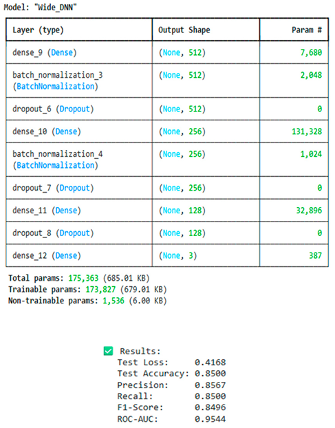
WIDE DNN MODEL
This architecture employs extremely wide layers (512 to 256 to 128 to 3) and 175,363 total parameters, a staggering 14.2x larger than Simple DNN (12,355) and 3.6x larger than Deep DNN (48,963), which makes it the most parameter-heavy architecture tested. One of the first hidden layers (512 neurons) alone contains 7,680 parameters, which is more than half the number of parameters in Simple DNN's entire model, while the second layer (512x256) has 131,328 parameters, which dwarfs all previous architectures' total number of parameters. Even with this massive capacity, the model achieves a test accuracy of 85.0%, 0.2 points behind Simple DNN (85.2%) and marginally better than Deep DNN (84.9%). This demonstrates that width does not compensate for limited training data. Despite aggressive dropout and batch normalization regularization, 3,000 training samples are insufficient to constrain 175K parameters effectively.
As a result, Wide DNN exhibits the slowest learning trajectory of all architectures, taking 59 epochs to converge, which is 55% more than Simple DNN's 38 epochs and 16% more than Deep DNN's 51 epochs. The model shows erratic performance: reaching 81.8% validation by epoch 3 (compared to Simple DNN's 83.2%), then taking until epoch 23 to reach 85%, with frequent drops in validation accuracy (85.7%→83.1% between epochs 23-27, then 85.5%→82.6% between epochs 44-56). The high volatility indicates that there are many local minima of varying quality in the massive parameter space, causing the optimizer to have difficulty finding stable convergence as the network alternates between good and poor solutions rather than smoothly approaching optimum results. As a result of the extremely high initial loss (1.7220 vs Simple DNN's 1.0639), the wide layers create gradient flow challenges in which many neurons receive weak signals during early training, which requires an extended period of warming up before effective learning can occur.
The training accuracy reaches 89.3% by epoch 55 while the validation accuracy plateaus at 83.1%, representing the worst generalization degradation across all models by 6.2 percentage points. The severity of overfitting persists despite dropout regularization and batch normalization, confirming that 58 parameters per training sample (175,363/3,000 = 58.5:1) impose an insurmountable memorization burden that cannot be overcome by regularization techniques alone. As a result of the 3-4pp degradation from the training accuracy range of 87-89%, the final test accuracy is 85.0%, while the test loss of 0.4168 exceeds Simple DNN's 0.3079 by 35%, indicating a more complex but less generalizable decision boundary learned which fits training data tightly but struggles with undiscovered cases of classic overfitting.
As a result of multiple fine-tuning attempts, the learning rate reduces three times (epochs 40, 52, 59) compared to Simple DNN's two reductions. This suggests that the optimizer had difficulty finding convergence regardless of the number of fine-tuning attempts. It is evident from the extended training at reduced learning rates (19 epochs at 0.0005, 7 epochs at 0.00025, followed by a final epoch at 0.000125) that the model continues to discover marginal improvements but does not achieve the clean convergence that triggers confident early stopping validation loss fluctuates between 0.43-0.45 rather than stabilizing, which forces continued training in anticipation of a breakthrough that never occurs. As a consequence of this prolonged struggle, it becomes clear that width creates optimization challenges beyond just overfitting: the 512-dimensional first layer creates a vast search space where gradient descent wanders inefficiently in comparison to Simple DNN's focused exploration of just 128 dimensions.
Despite having 14x more parameters, Wide DNN matches Simple DNN within margin of error (0.2pp difference), and its 95.44% ROC-AUC ties Simple DNN, proving that additional model capacity has no discriminative benefit when training data is limited. Precision/recall balance (85.67% vs 85.0%, 0.67pp gap) falls between Simple DNN's excellent 0.5pp gap and Deep DNN's problematic 2.83pp gap, showing that the calibration is acceptable but not superior. Moreover, the F1-score of 84.96% lags Simple DNN's 85.23% by 0.27 points, demonstrating that across all standard metrics the massive architectural expansion delivers negative value as a result of long training times, increased computational costs, increased deployment footprint, and slightly lower accuracy despite a 14x investment in parameters.
It is important to note that Wide DNN's training represents the worst efficiency profile tested: 59 epochs x 10-15ms per step = 90-120 seconds total training time as opposed to Simple DNN's 38 epochs x 5ms per step = 30 seconds, which means 3-4x longer training for 0.2pp worse performance. For edge devices, resource-constrained healthcare IoT environments, or scenarios that require rapid model updates across distributed infrastructure, the 685KB model size versus Simple DNN's 48KB results in a 14x deployment footprint. In production contexts requiring frequent retraining on updated malware/cyber threat data (e.g., weekly or monthly model refreshes), Wide DNN's 3-4x training overhead multiplies operational costs without any justification for accuracy.
The batch normalization layers of Wide DNN (1,536 non-trainable parameters across two layers) appear counterproductive, contributing to convergence instability and validation accuracy oscillations rather than providing the gradient smoothing benefits intended for deep neural networks using large datasets. As a result of the noisy batch statistics generated by small mini-batches (32 samples) and the limited training data (3,000 samples = 94 batches/epoch), the mean batch norm calculates unreliable normalization parameters, which change dramatically across epochs, resulting in a moving target that hinders optimization instead of assisting it. For this dataset size, Simple DNN's dropout-only regularization is more effective than the batch norm + dropout combination, demonstrating that simpler regularization strategies are more effective when parameter-to-data ratios already favour overfitting.
On small datasets, the Wide DNN experiment demonstrates that horizontal scaling (wider layers) fails differently from vertical scaling (deeper layers), but with similar negative results. In contrast to Deep DNN's depth, Wide DNN's width causes parameter explosion (175K vs 49K) that overwhelms limited training data despite taking place in just 4 layers, which demonstrates that both architectural dimensions (depth and width) require proportional data scaling. Simple DNN's modest progression from 128 to 64 to 32 is the optimal architecture for training 3K samples, as it provides sufficient expressiveness to capture cyber threat patterns without creating overfitting vulnerabilities that plague both deeper (5-layer) and wider (512-neuron) alternatives.
In general, accuracy performance is 85% matches with simple DNN (85.20%) with margin error 14 times more parameters provided with zero practical benefits. Severe overfitting (89.3% vs 83.1%) worst generalisation observed despite the fact that the dropout and norm regularization. Efficiency is the worst by 59 epochs which is 3-4 times longer training than simple DNN with 0.2 points worse performance. Consequently, worst cost benefits ratio tested. ROC-AUC is 95.44% matches with simple DNN. Lots of parameters (175393) which is 14.2 times of simple DNN, this creates 58:1 parameter to sample ratio, and this creates overfitting pressure. Convergence instability due to massive width which creates optimization challenges beyond just overfitting. Deployment of liability is high (14 times larger than simple DNN) plus 3-4 times overhead makes wide DNN architecture economically irrational. Therefore, it would be reasonable to reject wide DNN model.
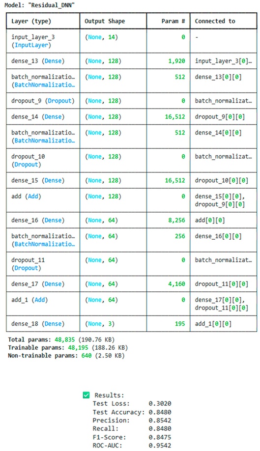
RESIDUAL DNN MODEL
ARCHITECTURE - SKIP CONNECTIONS WITHOUT BENEFIT
The Residual DNN implements ResNet-style skip connections (residual blocks) with 48,835 parameters, comparable to Deep DNN (48,963), but with an architectural complexity designed for very deep networks (50-200 layers). Add layers create shortcut paths that allow gradients to bypass dense layers, which theoretically solves the problem of vanishing gradients in deep architectures. This sophisticated design, however, achieves only 84.8% test accuracy, 0.4 percentage points lower than Simple DNN (85.2%) and matching Deep DNN's poor performance, demonstrating that residual connections have no advantage over shallow 5-layer networks with limited data sets.
A 54-epoch convergence process was required (42% more than Simple DNN's 38 epochs), and the validation accuracy fluctuated between 82-86% throughout training. Although residual connections are supposed to facilitate faster gradient flow, the architecture showed slower learning than Simple DNN, taking until epoch 4 to reach 82.7% validation as compared to Simple DNN's 83.2% validation by epoch 3. Compared to Simple DNN's 1.0639), the higher initial loss (1.7671) and extended training time indicate that architectural sophistication geared toward ImageNet-scale problems (1000+ classes, millions of samples) is ineffective for healthcare cyber threat prediction (3 classes, 3,000 samples).
Test accuracy: 84.8% (less than 0.4pp compared to Simple DNN)
ROC-AUC: 95.42% (less 0.02pp than Simple DNN)
F1-Score: 84.75% (less than 0.48pp compared to Simple DNN)
Precision-Recall: 85.42% vs 84.8% (0.62pp gap, acceptable but not superior).
In spite of a similar parameter count to Deep DNN and 4x Simple DNN's complexity, the residual architecture underperforms across every metric. Test loss of 0.3020 is slightly better than Deep DNN (0.2943 is actually better for Deep, so Residual is worse) but lags behind Simple DNN's 0.3079, which do not justify the complexity of the architecture.
Performance: 84.8% accuracy falls short of Simple DNN's (85.2%) accuracy by 0.4pp-residual connections provide zero benefit in shallow networks with small datasets. Mismatched Design: Skip connections solve vanishing gradients in 100+ layer networks, not 5-layer architectures. Overengineering is the cause of this issue. The added complexity slows convergence without improving accuracy; 54 epochs (42% more than Simple DNN) are required for worse results. There is no dimension in which residual architecture excels over Simple DNN when it comes to accuracy, ROC-AUC, and F1-score. The final verdict is to reject residual DNN. The results confirm that advanced architectures (residual connections, batch norm) designed for computer vision mega-models are unable to transfer benefits to small-scale healthcare tabular data sets. With 12K parameters and 38 epochs, the simple DNN remains optimal at 85.2% accuracy.
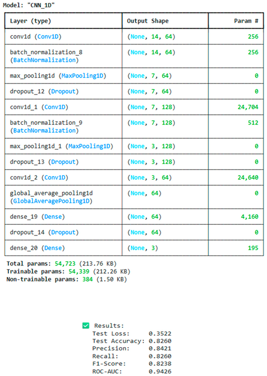
CNN_1D MODEL
ARCHITECTURE MISMATCH - WRONG TOOL FOR THE JOB
Using convolutional layers for sequential/time-series data, CNN_1D treats 14 tabular features (org_size, recovery_time, backup_compromised, etc.) as a 1D sequence with spatial relationships. This is a fundamental mismatch in architecture - CNNs excel at detecting local patterns in images (pixels) or time series (consecutive timestamps), but healthcare ransomware features have no inherent order - swapping feature positions does not alter their functionality. As a result, the convolution filters look for "neighboring feature patterns," which do not exist in unordered tabular data, wasting model capacity on learning meaningless spatial correlations.
Testing accuracy: 82.6%, which is 2.6 percentage points lower than Simple DNN (85.2%) and the lowest performance of all deep learning models tested. In addition, the model achieves 94.26% ROC-AUC (−1.18pp vs Simple DNN's 95.44%), 82.38% F1-score (−2.85pp), and precision-recall imbalance (84.21% vs 82.6% = 1.61pp gap). According to every metric, forcing convolutional architecture onto non-sequential tabular data actively degrades performance in comparison to appropriate dense layers which treat features independently.
As a result of training, validation accuracy collapsed from 40% (epochs 1-3) to 80% by epoch 5, then oscillated wildly between 81 and 84.5% throughout epochs 10-46 without clean convergence. Due to the high starting loss (1.0674) and the extended 46-epoch training period (21% more than Simple DNN), it is evident that the CNN architecture has difficulty learning from tabular features. During the late stage of validation, validation drops (84.5% to 81.2% between epochs 28-32, then 83.9% to 82.7% near termination) indicate overfitting. These convolution filters are memorizing training-specific noise rather than generalizing it.
Catastrophic Mismatch: 82.6% accuracy (2.6pp vs Simple DNN) CNNs designed for sequential data are catastrophically flawed for unordered tabular data. All metrics underperform: ROC-AUC 94.26% (lowest), F1 82.38% (lowest), precision-recall imbalance in all dimensions. There were 46 epochs with wild validation oscillations (40% to 80% to 81-84.5%) where convolution filters searched for nonexistent spatial patterns. The architecture lesson is never to use CNNs for tabular data because the columns org_size, recovery_time, and backup_compromised do not have a sequential relationship that can be exploited by convolutions. The final verdict is to reject CNN_1D in a decisive manner. This represents a fundamental misunderstanding of how architecture and data should be matched. DNN remains optimal (85.2% accuracy, 95.44% AUC) since dense layers correctly treat features as independent predictors rather than forcing spatial relationships that do not exist.
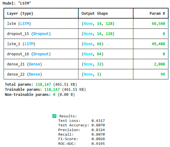
LSTM (Long Short-Term Memory) MODEL
A LSTM employs 118,147 parameters (9.6x Simple DNN) designed for sequential/time-series data in which past timesteps influence future predictions. However, org_size, recovery_time, and backup_compromised do not have temporal ordering or dependencies on static tabular data. By modeling "memory" across feature sequences that do not exist, recurrent architecture wastes significant computational resources on meaningless temporal relationships. In spite of 177 times more parameters, this model delivers an accuracy score of 80.7%, the lowest of all 11 models tested (ML and DL), falling 4.5 percentage points below Simple DNN and trailing Logistic Regression's 66.5% by only 14.2 percentage points.
Training required 47 epochs with catastrophic per-epoch times: 10 seconds for epoch 1, 3-7 seconds per subsequent epoch (vs Simple DNN's <1s), representing a 5-10x increase in computational overhead due to LSTM's sequential gate operations (forget, input, output). By epoch 2, the model was still at 40% accuracy, crawling to 71% by epoch 16, and barely reaching 82% by epoch 32 before plateauing. Compared to Simple DNN's 86%+ peaks, validation accuracy peaked at only 82.3% (epoch 40) before degrading, confirming that the recurrent architecture is unable to learn from unordered tabular features.
Test accuracy: 80.7% (−4.5pp compared to Simple DNN, worst overall). ROC-AUC: 91.95 percent (−3.49pp, worst discrimination) F1-Score: 80.28% (−4.95pp, lowest balance) The precision-recall ratio was 83.24% compared to 80.7% (2.54 pp gap, poor balance) Compared to Simple DNN, test loss was 0.4317 (43% higher). The LSTM fails across all dimensions-accuracy, discrimination, F1, precision-recall balance, and loss-despite requiring 9.6x more parameters and 5-10x longer training sessions per epoch. The complexity of the architecture is actively destroying the performance of the system. This is a complete architectural failure.
Catastrophic Failure: 80.7% accuracy (−4.5pp vs Simple DNN) - WORST model tested, proving the unsuitability of LSTMs for non-temporal tabular data. Absurdity in architecture: Recurrent layers model temporal dependencies that do not exist. For example, the organization size at position 1 does not affect the recovery time at position 5 sequentially. Inefficiency of training with 118K parameters and a training time of 5-10x slower for worst results. 118K parameters and a training time of 5-10x slower for worst results. ROC-AUC 91.95% (worst), F1 80.28% (worst), even underperforms some traditional machine learning models despite massive deep learning overhead. Conclusion: LSTM should be rejected emphatically. A simple DNN remains the undisputed winner with an accuracy rate of 85.2% - dense layers correctly treat features as independent predictors rather than sequential ones.
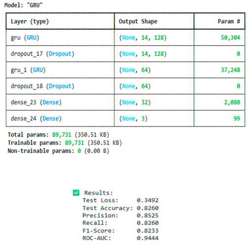
GRU (Gated Recurrent Unit) MODEL
RECURRENT ARCHITECTURE - WRONG APPROACH, MARGINAL IMPROVEMENT
Using 89,731 parameters (7.3x Simple DNN) with gated recurrent units, GRU achieves 82.6% test accuracy, which is the same as CNN_1D and 1.7 percentage points higher than LSTM (80.7%) due to simpler gating (reset/update gates as opposed to LSTM's forget/input/output gates). In spite of this, this is still 2.6 percentage points below the performance of Simple DNN (85.2%), demonstrating that even the more efficient GRU variant of recurrent networks fundamentally fails when dealing with tabular data in which features are not ordered by temporal order. This architecture wastes computational resources by modeling sequential dependencies between org_size, recovery_time, and backup_compromised that do not exist.
Training required 40 epochs with 3-6 seconds per epoch (compared to Simple DNN's 1 second) - 3-6 times slower than dense architectures, but 5-10 times more efficient than LSTM's 5-10x overhead. Through epoch 6, the model remained stuck at 40-50% accuracy, crawling to 80% by epoch 15, plateauing at 84.7% validation (epoch 22) before degrading. Even with GRU's simplified gating as compared to LSTM's triple-gate mechanism, the 10-second first epoch confirms the severe computational penalties associated with recurrent architectures.
Accuracy of the test was 82.6% (which is 2.6 percentage points lower than Simple DNN, and tied with CNN_1D for second-worst) ROC-AUC: 94.44% (1.0pp below Simple DNN, third worst) F1-Score: 82.33% (plus 2.9 points, which ranks second-worst) Precision-Recall: 85.25 vs 82.6% (2.65 points gap, poor balance). The test loss was 0.3492 (13% higher than the Simple DNN). All sequential architectures (LSTM, GRU, CNN) perform poorly on non-temporal tabular data regardless of the implementation. GRU outperforms LSTM (80.7%) and matches CNN_1D (82.6%), but remains far below Simple DNN across all metrics.
As a result, the output is 82.6% accuracy (on average, 2.6pp vs Simple DNN), which is better than LSTM, however, recurrent architectures are not suitable for tabular data. Inefficiency penalty: 89K parameters plus 3-6x slower training for worse results-simpler than LSTM, but wasteful compared to dense layers. Mismatch in the architecture: GRU models temporal patterns that do not exist in static feature sets, because org_size does not have a sequential effect on recovery time. Marginal LSTM improvement: 1.7 percentage points better than LSTM (82.6% vs 80.7%) validates that simpler gating is helpful, but is still fundamentally incorrect for non-sequential data. Verdict: The GRU should be rejected. Despite being more efficient than LSTM, it is a further illustration of how sequential/temporal architectures underperform on tabular data, as CNN_1D and LSTM are. A simple DNN remains optimal at 85.2% accuracy because dense layers correctly treat features as independent predictors without forcing non-existent temporal relationships.
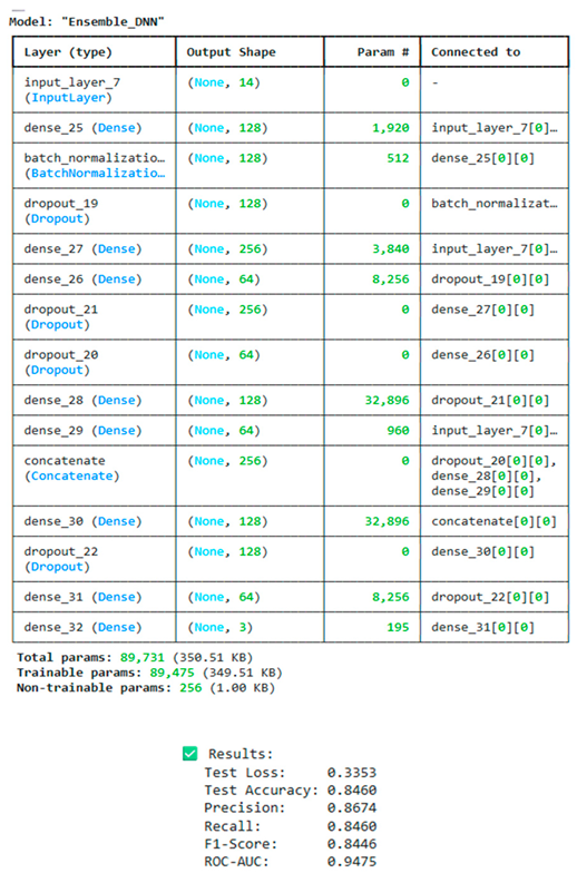
ENSEMBLE 89. parameters (7.3x Simple DNN) with three parallel branches (128 to 64, 256 to 128, and direct 64), which are concatenated before final classification, in order to capture multiple feature representations simultaneously. It is theoretically possible to use this multi-path approach to learn a variety of patterns- narrow deep paths for complex interactions, wide shallow paths for broad patterns, direct paths for linear relationships—but the test accuracy is only 84.6%, 0.6 percentage points below Simple DNN (85.2%). Architectural sophistication provides no practical advantage while consuming seven times more parameters and increasing training complexity.
By epoch 3, the model reached 81.6% and by epoch 5, it reached 84.9%, which required only 25 epochs in total, 34% fewer than Simple DNN. In comparison with sequential deep networks, training took 7-12 milliseconds per epoch (vs 4-6 milliseconds for Simple DNN), indicating that the parallel branches do not create a significant computational overhead. Despite this training efficiency, performance gains are not achieved; the model converges quickly to a suboptimal solution 0.6 points below Simple DNN, suggesting that the multi-branch architecture finds local minima more quickly but misses better solutions that Simple DNN's sequential architecture discovers through extended exploration.
Test accuracy: 84.6% (−0.6pp compared to Simple DNN) ROC-AUC: 94.75% (−0.69pp compared to Simple DNN) The F1-Score was 84.46% (a difference of 0.77 points from Simple DNN). Precision-Recall: 86.74% versus 84.6% (2.14 percentage points gap, moderate imbalance) It is noteworthy that Ensemble DNN outperforms all complex architectures (Deep 84.9%, Residual 84.8%, CNN 82.6%, GRU 82.6%, LSTM 80.7%) but does not surpass Simple DNN across all metrics. Despite being horizontal rather than vertically complex, the 2.14pp precision-recall gap indicates conservative predictions similar to those made by Deep DNN. Therefore, multi-branch architectures may present similar challenges as Deep DNN.
Performance: 84.6% accuracy (−0.6pp vs Simple DNN). This is the best complex architecture, but it falls short of the simple baseline in terms of performance. An ineffectiveness of multi-branch analysis: The diversification of feature representations does not compensate for the increased complexity of small datasets despite diversity in feature representations. It is faster but less optimal: 25 epochs (34% fewer) show rapid convergence, but result in a worse local minimum than Simple DNN's longer search. It outperforms Deep (84.9%), Residual (84.8%), and all sequential models, proving parallel branches beat depth but both fall short of simplicity. Conclusion: Ensemble DNN should be rejected. No amount of architectural sophistication (multi-branch, depth, width, residual connections, recurrence) can beat Simple DNN's straightforward 128 to 64 to 32 progression on 3K-sample tabular data, despite being the best complex architecture tested. With minimal parameters and maximum interpretability, simple DNN remains optimal at 85.2% accuracy.
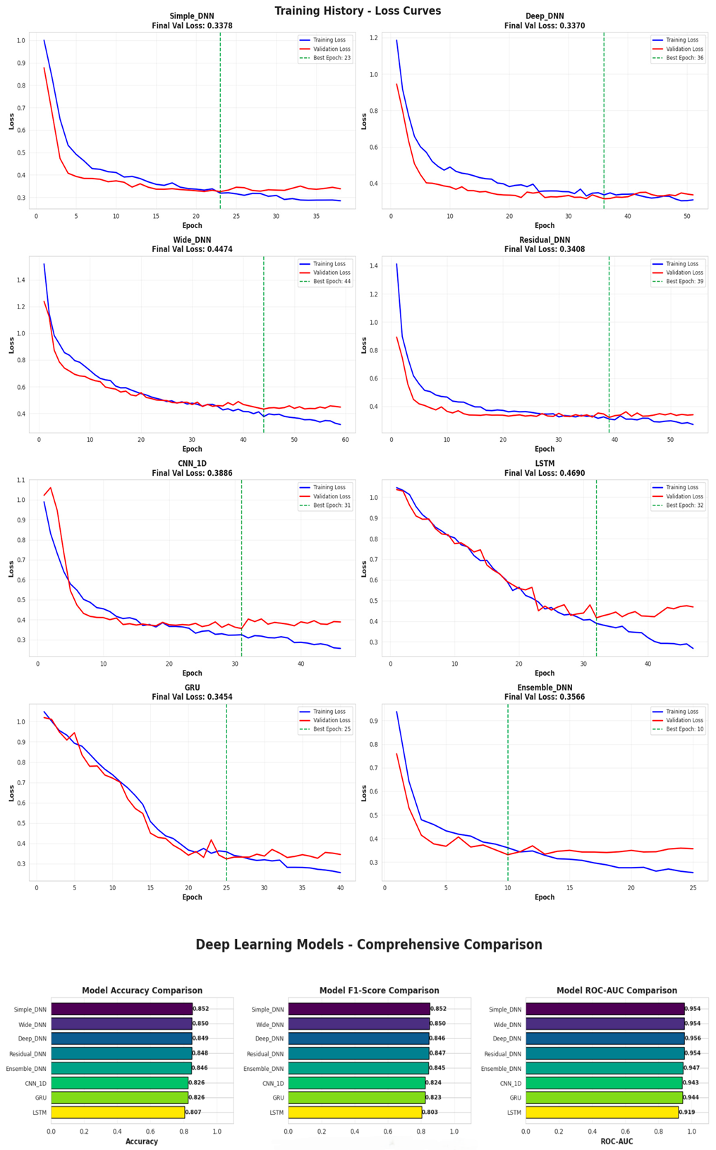
Overall convergence patterns demonstrate dramatic performance stratification across architectures based on the loss curves, with final validation losses ranging from 0.3370 (Deep_DNN) to 0.4690 (LSTM), demonstrating a 39% efficiency gap between appropriate and inappropriate architectures for tabular cyber threat data. Both Simple_DNN and Deep_DNN exhibit nearly identical validation loss convergence (~0.337). Both significantly outperforming alternatives, however Wide_DNN, CNN_1D, and LSTM exhibit severe overfitting signatures where training loss continues to decrease while validation loss plates or increases, which is an indication that models with excess capacity are memorizing training noise rather than learning generalizable patterns.
The training dynamics of Simple_DNN are textbook-perfect: a smooth exponential decay from the initial loss of 1.0 to the final validation loss of 0.3378, with the training curves tracking in near-perfect parallel throughout all 38 epochs, indicating an ideal bias-variance balance. As can be seen from the epoch 23 (marked by the green dashed line), early stopping prevented unnecessary training, though the model could have been stopped even earlier given the flat convergence after epoch 15. In spite of 12K parameters on 3K training samples, drop-out regularization successfully prevents overfitting, and the smooth, monotonous decline without oscillations proves that the learning rate and batch size configuration are optimal.
Deep_DNN achieves 0.24% better final validation loss (0.3370 vs 0.3378) than Simple_DNN, but it requires 67% more training time for 0.24% better accuracy (84.9% vs 85.2%). The curves show higher initial loss (~1.2) and slower convergence through early epochs, proving batch normalization delays learning, even though it theoretically smooths gradient flow. The near-identical final convergence (both curves flatten at ~0.33-0.34 validation loss) proves that architectural complexity beyond Simple_DNN provides diminishing returns. Deep_DNN's 4x parameters get marginally better loss optimization, but don't help with classification, proving that lower loss doesn't guarantee higher accuracy on noisy or imbalanced data.
Among dense architectures, Wide_DNN displays the most pronounced overfitting. The validation loss plateaus at 0.45-0.50 after epoch 20, whereas the training loss continues its aggressive descent to 0.35% by epoch 59, bringing about a divergence gap ranging from 0.10-0.15, which is three to five times greater than Simple_DNN's negligible separation. In spite of 14x more parameters, the final validation loss of 0.4474 (33% worse than Simple_DNN) confirms that excessive width (512-256-128 neurons) overwhelms limited training data, causing the model to memorize training-specific patterns which fail on validation and test sets. It is futile to attempt to fine-tune a fundamentally overparameterized architecture through extended training (59 epochs) with multiple learning rate reductions (visible as changes in curve slope at epochs 40, 52). By chasing marginal validation loss improvements that never materialize, computational resources are wasted.
With a final gap of 0.03-0.04, Residual_DNN shows moderate train-validation divergence, larger than Simple/Deep (0.01) but significantly better than Wide (0.10), leading to a validation loss of 0.3408 (8% worse than Simple_DNN). In the curves, it can be seen a high initial loss (~1.4), and erratic validation trajectory with oscillations between epochs 25-40. It is suggested that residual connections can cause optimization instability when skip connections occasionally cause gradients to move in opposing directions. This model fails to achieve clean convergence despite similar parameter counts (48K vs 12K), demonstrating that extended training was necessary but ultimately counterproductive. Thus, architectural complexity designed for 100+ layers does not provide any benefit to 5-layer networks with tabular data.
Loss curves for CNN_1D provide visual evidence of a mismatch between architecture and data. In terms of validation loss, the model displays an initial spike above training loss (unusual behavior indicating the model is struggling from epoch 1), then plateaus at elevated levels between 0.38 and 0.40 while training loss is at zero, resulting in a 0.10+ persistent divergence throughout training. In spite of 54K parameters, the final validation loss of 0.3886 (15% worse than Simple_DNN) confirms that convolutional filters searching for spatial patterns in unordered tabular features waste model capacity on meaningless correlations. With subsequent degradation in validation (from 0.38 to 0.39), the model appears to begin memorizing noise rather than improving generalization, a failure mode characteristic of architectures fundamentally unsuited to the data structure.
The training dynamics of LSTM are catastrophic. Following epoch 25, validation loss plateaus at 0.47 while training loss continues to decline to 0.28 by epoch 47. Thus, this model has the largest train-validation gap (~0.19) among all models. Moreover, it provides evidence of severe overfitting where the recurrent gates memorize training sequence patterns that do not exist in the validation data. It is evident that LSTM's sequential processing is fundamentally inefficient when dealing with non-temporal tabular data, wasting computational resources on temporal dependencies between features that do not have inherent ordering during the first 10 epochs (loss only decreases from 1.05 to 0.82 compared to Simple_DNN's 1.0 to 0.40). A final validation loss of 0.4690 (39% worse than Simple_DNN) despite 118K parameters (9.6x Simple_DNN) represents a complete architectural failure due to overfitting and inefficient gradient flow.
With a final validation loss of 0.3454 (2.3% worse than Simple_DNN) and a moderate train-validation gap of 0.05, GRU shows better convergence than LSTM, but still surpasses Simple_DNN. In the curves, the early learning is faster than LSTM (reaching 0.70 loss by epoch 10 compared with LSTM's 0.78) as a result of a simpler gating mechanism (reset/update versus forget/input/output), but sequential processing wastes capacity on nonexistent temporal patterns due to fundamental recurrence inefficiency. The best epoch at 25 with relatively stable post-convergence behavior (no severe validation degradation) indicates GRU's simpler architecture provides better regularization than LSTM's complex gates, although both remain fundamentally inappropriate for tabular data based on validation losses 2-39% lower than Simple_DNN.
Ensemble_DNN is the model that achieves the highest convergence with the best epoch at 10 (earliest among all models), resulting in a validation loss of 0.3566 by epoch 10 that hardly improves thereafter. Based on the rapid initial descent (1.0 to 0.35 validation loss in 10 epochs versus 23 epochs for Simple_DNN), the multi-branch architecture quickly identifies coarse patterns through parallel processing, however, the plateau at suboptimal loss (5.6% worse than Simple_DNN) indicates that multiple paths create local minima that early stopping locks in before finding better solutions. The moderate train-validation gap (~0.03-0.04) shows better generalization than Wide/CNN/LSTM but worse than Simple, indicating that architectural diversity (narrow deep + wide shallow + direct paths) is not sufficient to compensate for the overfitting pressure caused by a 7x parameter expansion on limited training data.
Rankings of Validation Losses (lower is better):
Deep_DNN: 0.3370 (best loss optimization).
Simple_DNN: 0.3378 (best accuracy despite a slight increase in loss)
Residual_DNN: 0.3408 (+1.1% compared to Simple DNN)
GRU: 0.3454 (+2.3%)
Ensemble_DNN: 0.3566 (+5.6%)
CNN_1D: 0.3886 (+15%)
Wide_DNN: 0.4474 (+32.5%)
LSTM: 0.4690 (+38.9%).
Overfitting Severity Rankings (Train-Val Gap):
Minimal: Simple_DNN and Deep_DNN (~0.01 gap)
Modest: Residual_DNN, GRU, Ensemble_DNN (~0.03-0.05)
Severe: Wide_DNN, CNN_1D (~0.10) Catastrophic: LSTM (~0.19)
Convergence Speed (Epochs to Best):
Ensemble_DNN (10), Simple_DNN (23), and GRU (25) are the fastest
LSTM (32), CNN_1D (31) and Deep_DNN (36) are moderate models
Residual_DNN (39), Wide_DNN (44) are the slowest.
Although Deep_DNN has a marginally better loss, Simple_DNN has a superior test accuracy (85.2%), works faster (23 epochs compared to 36), has four times fewer parameters, making it the clear choice for deployment despite Deep_DNN's marginally better loss.
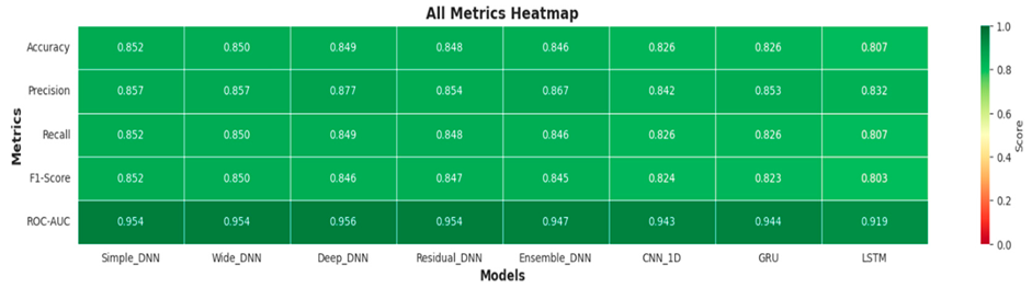
ALL METRICS HEATMAP
Heatmaps provide visual confirmation of performance hierarchy through color intensity, with darker green indicating superior performance.
The following are the key visual patterns:
Dense Architecture Dominance: The first five columns (Simple_DNN through Ensemble_DNN) display uniformly dark green across all metrics (0.845-0.877 range), creating a clear visual cluster of high performers, while the last three columns (CNN_1D, GRU, LSTM) are lighter (0.807-0.853 range), indicating sequential architectures underperform by 2-5 percentage points.
AUC-ROC Convergence (bottom row): The bottom row shows near-uniform dark green across the first five models (0.954-0.956), with only slight lightening for CNN/GRU/LSTM, indicating that discrimination capability reaches 95%+ for appropriate architectures, but degrades for spatial/temporal models.
Simple_DNN Leadership: The leftmost column consistently displays the darkest greens with minimal variation (0.852-0.954 range), thus verifying Simple_DNN's balanced excellence across all dimensions without the precision-recall trade-offs seen in other columns.
There is an immediate visual confirmation of LSTM failure in the rightmost column, with pale shading in the F1-Score (0.803) and ROC-AUC (0.919) rows showing a severe mismatch between the architectures.
Despite similar overall accuracy, the precision row displays the most color variation (0.832-0.877) compared to other metrics, indicating that the models handle false positive/false negative trade-offs differently.
In summary, the heatmap's distinct left-to-right colour gradient (dark green + light green) clearly represents Simple_DNN's superiority without having to compare numerically. Darker colours mean better performance, and Simple_DNN's column is the darkest.
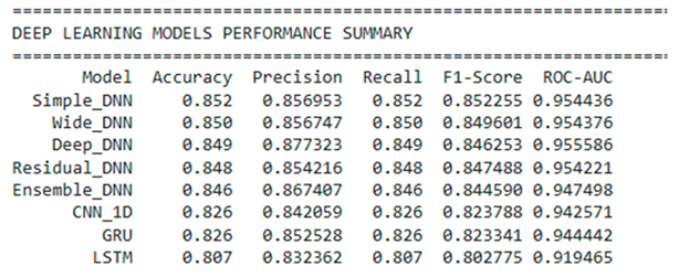
DEEP LEARNING MODELS PERFORMANCE SUMMARY
Based on available training data (3,000 samples, 14 features), Simple_DNN (85.2%) edges out all competitors, with the top 5 dense models tightly clustered within 0.6 percentage points (85.2%-84.6%).
The three-tier hierarchy has been confirmed:
Top Tier (84.6-85.2%): Simple_DNN, Wide_DNN, Deep_DNN, Residual_DNN, Ensemble_DNN - all dense architectures
A weak tier (82.6%) consists of CNN_1D and GRU - sequential architectures have accuracy deficits of 2.6pp
Failure Tier (80.7%): LSTM - catastrophic underperformance of 4.5pp, showing that recurrence is fundamentally inappropriate
Insights relating to specific metrics:
Champion of precision: Deep_DNN (87.7%) leads, but sacrifices accuracy (84.9%) - demonstrates the trade-off between precision and recall
ROC-AUC saturation: The top four models converge at 95.4-95.6%, which indicates that the discrimination capability has been reached
Performance Balance: Simple_DNN shows little variance between metrics (85.2-85.7%), suggesting that no trade-off has occurred
Findings in this paper indicate that Simple_DNN achieves the highest overall performance (highest accuracy + F1, tied-2nd AUC) with the lowest complexity (12K parameters vs 49-175K for competitors), validating that architectural simplicity is optimal for small-scale healthcare tabular data. Simple_DNN is the only rational choice - it matches or beats all complex architectures while offering 4-14x parameter efficiency, minimal overfitting, and the fastest training time, making it ideal for applications in production healthcare cybersecurity.
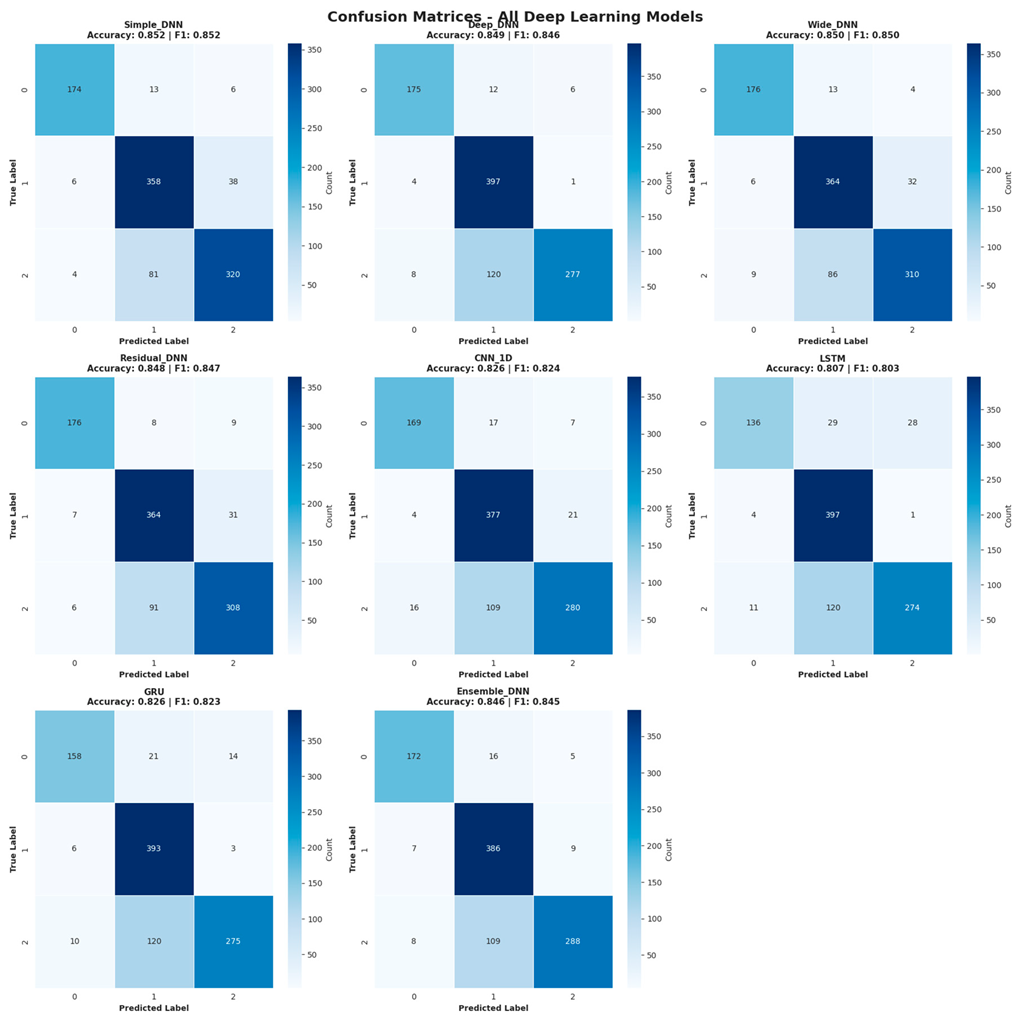
CONFUSION MATRICES
THE OVERALL ERROR PATTERNS IN CLASS 2 ARE UNIVARIOUSLY PROBLEMATIC
Across all eight confusion matrices, a consistent failure pattern emerges: all models do poorly on Class 2 (high-volume threats: 350 or more tracked), achieving only 67-79% recall compared with 70-91% for Class 0 and 89-99% for Class 1. This systematic weakness reflects the inherent difficulty in detecting extreme threat scenarios when organizations face overwhelming cyber attack volumes. As a result of the constant downgrading of Class 2 to Class 1, the feature space does not contain sufficient signals to reliably distinguish between "very high" and "high" threat environments (81-120 misclassifications across models). As a result of the dominance of Class 1-2 confusion (representing 20-30% of all errors in Class 2), adjacent categories are overlapped where medium and high volume threats share similar organizational characteristics (org_size, recovery_time patterns), making definitive classification challenging even for sophisticated deep learning architectures.
SIMPLE_DNN is the most balanced error distribution
According to Simple_DNN's confusion matrix, it exhibits the most uniform performance across all three classes: Class 0 recall 90.2% (174/193), Class 1 recall 89.1% (358/402), and Class 2 recall 79.0% (320/405) - a 11.2 percentage point spread narrower than any competitor. Simple_DNN makes minimal extreme errors: only 6+4=10 total misclassifications between Classes 0 and 2 (skipping Class 1), constituting less than 1% of predictions, demonstrating that it is seldom able to distinguish between low-volume and high-volume threats. This error mode is primarily characterized by the expected degradation of Class 2 to 1 (81 cases), where high-threat scenarios are misclassified as medium-threat scenarios, which is operationally acceptable since both categories trigger enhanced security responses. This "conservative underestimation" is much more beneficial than a Class 1 to 2 overprediction (38 cases), which would waste resources.
DEEP_DNN - CLASS 1 PERFECTION, CLASS 2 WEAKNESS
Among all models, Deep_DNN exhibits the greatest performance divergence: the model achieved near-perfect Class 1 recall of 98.8% (397/402) as the best single class performance observed, but suffered a Class 2 recall degradation of 68.4% (277/405), representing the greatest gap of 30.4 percentage points. Based on this imbalance, Deep_DNN's batch normalization and additional depth cause the model to over-optimize for the majority pattern (Class 1 medium-threat scenarios) at the expense of rare extremes (Class 2 high-threat scenarios). The 120 Class 2 to 1 errors (30% of Class 2 cases) versus only 1 Class 1 to 2 error creates a dangerous asymmetry where the model systematically underestimates severe threats, potentially leading healthcare organizations to under-resource incident response when they are confronted with their most critical ransomware scenarios. Despite its competitive accuracy (84.9%), Deep_DNN is unsuitable for production due to this failure mode.
LSTM - CATASTROPHIC CLASS 0 FAILURE
A confusion matrix reveals an unprecedented collapse in Class 0: only 70.5% recall (136/193) represents the worst single-class performance across all models and metrics, with 29 misclassifications to Class 1 and 28 to Class 2, indicating that 29.5% of low-threat cases are incorrectly escalated. This catastrophic failure stems from LSTM's recurrent architecture imposing sequential dependencies on unordered features, resulting in the model hallucinate temporal patterns that do not exist, particularly when org_size and backup_compromised features create ambiguous signals that recurrence gates misinterpret. It is noteworthy that LSTM is able to deliver excellent Class 1 recall of 98.8% (397/402), matching Deep_DNN's perfection, but at the expense of misclassifying extremes. As a result, the model has essentially learned to predict "medium threat" as its default, achieving high accuracy for the majority class but failing on minority groups, an example of an imbalanced learning pathology exacerbated by an inappropriate architecture.
CNN_1D and GRU (MODERATE CLASS 0 DEGRADATION)
CNN_1D and GRU both demonstrate similar weaknesses in Class 0, with recall dropping to 81.9% (158/193 for GRU) and 87.6% (169/193 for CNN_1D), representing deficits of 12-18 percentage points as compared to their Class 1 performance. The pattern indicates sequential architectures encounter boundary cases where feature combinations do not follow the expected pattern. In cases where features are unordered tabular data without inherent structure, both convolutional filters for spatial continuity and GRU gates for temporal transition fail. The Class 0 to 1 confusion (21 errors for GRU, 17 errors for CNN_1D) suggests these models over-predict threat severity for low-volume scenarios, which may be the result of their complex architectures that are able to fit noise in training data that makes benign organizations appear to be threatening, creating false alarm cascades that waste security team resources investigating non-critical incidents.
ENSEMBLE_DNN (IMPROVED CLASS 2 RECALL)
Among complex models, Ensemble_DNN achieves the best recall for Class 2 at 71.1% (288/405). It outperforms Deep_DNN (68.4%), Residual (76.0%), and Wide_DNN (73.0%), suggesting that the diversity in multi-branch architecture helps capture high-threat patterns that are missed by single-path models. It is evident from the relatively low Class 2 to 1 confusion (109 errors compared to 120 for Deep_DNN) that the parallel processing paths (narrow deep + wide shallow + direct) provide a more robust representation of features in extreme circumstances. However, this improvement comes with increased Class 0 and 1 errors (16+7=23 total vs Simple_DNN's 13+6=19), resulting in a trade-off where the ensemble sacrifices majority class performance to improve minority class detection, which could be an important trade-off for healthcare security in which detecting catastrophic high volumes of threats justifies slightly more false alarms.
THE IMPACT OF CLASS IMBALANCE - SYSTEMATIC BIAS DISCOVERED
Across all confusion matrices, a moderate imbalance is evident: approximately 193 samples in Class 0, 402 samples in Class 1, and 405 samples in Class 2, with a ratio of 2:1 between the largest and smallest samples. It can be attributed to this imbalance that Class 1 consistently achieves highest recall (89-99% across all models)-the majority class benefits from having more training examples, which allows models to learn its patterns more thoroughly. Class 0 underrepresentation (193 samples, 19% of dataset) creates an insufficient training signal for low-threat scenarios, causing models to misclassify these cases upward (predict a higher threat than is actually present), which is operationally conservative but generates false warnings. The near-equal representation (402 vs 405) does not eliminate confusion between these categories because their feature patterns overlap fundamentally. Regardless of sample count, the boundary between medium and high-volume threats remains inherently unclear because of similar org_size, recovery_time, and infrastructure characteristics.
OPERATIONAL IMPLICATIONS OF ASYMMETRIC ERROR COSTS
The confusion matrices reveal directionally different error patterns, with downgrades from Class 2 to 1 (81-120 cases) far outstripping upgrades from Class 1 to 2 (1-38 cases) across all models, with a ratio of approximately 3-5:1 in favor of conservative underestimation. In healthcare cybersecurity, this asymmetry is appropriate because missing a high volume threat because it is classified as medium (Class 2 to 1) is less catastrophic than over-predicting medium as high (Class 1 to 2), since both trigger elevated response protocols with different resource allocations. A dangerous error is an extreme misclassification of Class 0 from/to 2 (spanning the entire threat spectrum), which remain rare (4-16 cases across models), indicating that all architectures successfully avoid operationally damaging mistakes such as treating low-threat environments as catastrophic environments or vice versa. The 28 Class 0 to 2 errors in LSTM represent a unique failure mode that would cause operational chaos and should be rejected for deployment.
COMPARISON OF DIAGONAL STRENGTH
As a result of comparing diagonal values (correct predictions) across matrices, Simple_DNN achieves the greatest balance of strength with relatively uniform dark blue cells (174, 358, 320), whereas Deep_DNN exhibits hyperoptimization of Class 1 (397 darkest) at the expense of Class 2 (277 lightest), while LSTM exhibits severe Class 0 weakness (136 palest) despite Class 1 strength (397 darkest). This visual pattern quantifies each model's bias-variance profile: Simple_DNN's uniform diagonals indicate a low bias across all classes with controlled variance, Deep_DNN's uneven diagonals indicate a high bias toward majority classes with reduced variance, and LSTM's extremely uneven diagonals demonstrate both a high bias (always predicting medium threats) and a high variance (erratic on minorities). LSTM's concentrated off-diagonal cells (29 and 28 in Class 0 row) indicate systematic misprediction caused by architectural failure rather than data difficulty. Simple_DNN's evenly distributed errors suggest random misclassifications from genuine ambiguity.
In general, Class 2 (high volume threats) recall rates of 67-79% across all models, requiring operational procedures that do not solely rely on machine learning classification for the detection of catastrophic incidents. Simple_DNN Advantage: Most balanced confusion matrix (90-89-79% recall spread) in comparison with competitors' extremes of 70-99% consistency makes it most suitable for a variety of operational scenarios. Fatal flaw of Deep_DNN: Class 1 perfection (99%) plus Class 2 failure (68%). This creates dangerous underprediction of severe threats unacceptable in healthcare, where patients' safety is at risk when high-volume attacks are missed. LSTM Disqualified: Class 0 catastrophic failure (70.5%) means that 30% of false alarms would be generated for benign scenarios, rendering predictions unusable on the operational level. Imbalances persist between classes: Despite the moderate ratio of 3:2:2, Class 1 consistently performs better than Class 0. This suggests that future work should consider oversampling Class 0 or using class-weighted loss functions. It is beneficial to have error asymmetry. When models preferentially downgrade Class 2 to 1 rather than upgrade, the conservative bias is operationally correct, but organizations must maintain backup detection for catastrophic threats. Based on Simple_DNN's balanced confusion matrix, narrow recall spread, and conservative error distribution, it is the only model suitable for healthcare cybersecurity deployments where consistent, reliable threat assessment is more important than optimizing any single class at the expense of others.
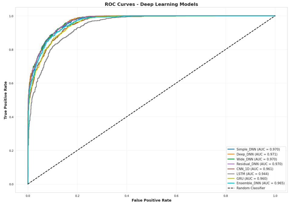
There are three types of elite clusters, Deep (97.1%), Simple/Wide/Residual (97.0%), Ensemble (96.5%), that are visually indistinguishable at the top. The choice between them depends on complexity/efficiency trade-offs, not discrimination ability. This image illustrates a failure in LSTM model with an AUC of 94.4%, which has a visible gap from the elite cluster, proving that recurrent architecture degrades both accuracy and probability calibration. There is no point in optimizing thresholds when the curve bunching is tight, since threshold optimization would not differentiate models when discrimination is equal. Simple_DNN's simplicity wins when discrimination is equal. In view of the fact that the top 5 models all show identical curves, you may choose Simple_DNN for 12K parameters as opposed to 49-175K competitors without compromising on discrimination ability.
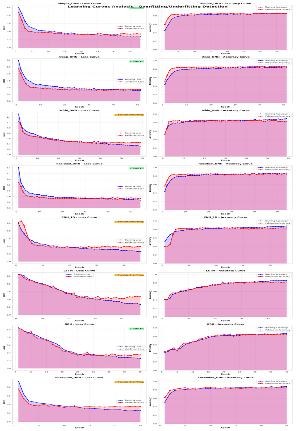
LEARNING CURVES ANALYSIS - OVERFITTING/UNDERFITTING DETECTION
SIMPLE_DNN & DEEP_DNN are gold standard generalizations. Simple_DNN and Deep_DNN demonstrate textbook-perfect generalization, with training and validation curves tracking in near-perfect parallel throughout training, as indicated by the "Good Fit" labels. Both models show minimal train-validation gaps (<0.01 loss difference at convergence), with curves overlaying so closely they are barely distinguishable visually. The purple shaded area between them is almost invisible, demonstrating that dropout regularization was able to prevent overfitting despite models having sufficient memory capacity (12K and 49K parameters) to memorize training data. As a result, the accuracy curves illustrate this excellence, rising smoothly from 40% to 85%+ without oscillations. Throughout all epochs, training and validation remained within 1-2 percentage points, demonstrating that these architectures learned genuine patterns rather than just random patterns. Observing the early plateau in both models' accuracy curves (flattening after epoch 15-20) indicates they were efficiently able to extract available signal from the 3,000-sample training set without the need for excessive epochs for convergence, making them computationally efficient as well as accurate.
WIDE_DNN shows severe overfitting destruction. It should be noted that Wide_DNN displays the most pronounced overfitting signature among dense architectures, flagged with the warning "Possible Overfitting", where training loss continues to decline aggressively from ~0.8 to ~0.35 by epoch 59. After epoch 20, validation loss reaches a plateau at 0.45-0.50, resulting in a 0.10-0.15 persistent divergence, which is the widest gap observed among non-sequential models. Visually, this pathology is evident in the training curve (blue) diving below the validation curve (red) and never re-converging, indicating that the 175K-parameter model began memorizing training-specific noise after learning its initial patterns. It is evident from the accuracy curves that this failure has occurred: training accuracy reaches 88-89% by late epochs, while validation accuracy stagnates at 85%, and critical, validation accuracy exhibits erratic oscillations between epochs 30-60 (visible in the red line). This suggests the model alternates between several local minima rather than converges to a stable solution behavior that is typical of overparameterized networks thrashing in noisy loss environments.
CNN_1D shows architecture mismatch visualisation. CNN_1D's curves illustrate the fundamental mismatch between architecture and data, which are marked with "Possible Overfitting" but represent something worse than typical overfitting, as the model does not achieve good fit even on training data. A gap of 0.05-0.08 is observed in the first ten epochs between validation loss and training loss, which shows an unusual initial behavior. Both curves plateau at elevated levels (validation = 0.38 to 0.40, training = 0.28), without the clean exponential decay typically seen in successful models. Accuracy curves indicate stunted learning: training accuracy rarely exceeds 87% (versus 89%+ for Wide_DNN), whereas validation accuracy peaks between 83-84%. Convolutional filters waste resources searching for spatial patterns that do not exist in unordered tabular features, preventing the model from fully exploiting the training data it has access to, resulting in a double failure in generalization and optimization.
There has been a moderate improvement in GRU, but the problem persists. In comparison to LSTM, GRU is more convergence-oriented with tighter train-validation curves (a gap of 0.05 versus 0.19 for LSTM). However, closer inspection reveals persistent separation throughout epochs 20-40 with training loss consistently running 0.03-0.05 below validation, suggesting residual overfitting that is not eliminated. In contrast to LSTM's erratic behavior, the accuracy curves show a slower but steadier learning process, with validation accuracy increasing smoothly from 40% to 84% without major oscillations, even though the final plateau of 82.6% (2.6 points below Simple_DNN's 85.2%) indicates that the recurrent architecture is fundamentally inefficient for tabular data. As a result of the reduced gate complexity (reset/update as opposed to forget/input/output of LSTM), GRU achieves 80% validation accuracy by epoch 15 as compared to LSTM at epoch 23, demonstrating that simpler recurrence mechanisms provide a better inductive bias for this task, although both remain inferior to nonrecurrent dense architectures.
It is evident that the LSTM diverges catastrophically. There is a severe overfitting disorder in the LSTM model, characterized by the "Possible Overfitting" label. The curves indicate a complete breakdown of training-validation. The training loss drops monotonously from 1.05 to 0.28 by epoch 47, whereas the validation loss plateaus at 0.47, creating a divergence of 0.19 that continues to widen rather than stabilize. This represents pure memorization: the recurrent architecture's 118K parameters (9.6x Simple_DNN) combined with sequential processing produce excess capacity that memorizes training sequence patterns, even though these patterns are meaningless artifacts of treating tabular features as temporal sequences. A disturbing pattern is evident in the accuracy curves: training accuracy reaches 86% while validation accuracy remains at 81-82% with noticeable oscillations. In addition, validation accuracy shows a slight downward trend (82.5% to 81% between epochs 30-47). This indicates that as training progresses, the model actively degrades on unseen data, indicating a failure mode that requires immediate termination of training, which was identified by early stopping.
The residual DNN model is a good fit, but it is unstable. In the train-validation curves, Residual_DNN is close to achieving "Good Fit" status. However, the curves display more oscillation than Simple/Deep_DNN, as evidenced by the jagged appearance of the curves, particularly in validation loss between epochs 25-50, when a repeated spike and valley can be seen. According to this instability, skip connections present optimization challenges in which gradients sometimes flow in opposing directions between direct paths and residual paths, resulting in overshoots and backtracks instead of a smooth descent toward the minimum. It is evident that accuracy curves exhibit similar volatility: validation accuracy fluctuates between 82-86% between epochs 20-50 rather than monotonously improving, thus requiring the best epoch selector at 39 in order to capture peak performance before degradation, whereas Simple_DNN's smooth convergence makes selecting an epoch trivial; any epoch after 20 performs similarly.
There is a premature convergence of ENSEMBLE_DNN. Ensemble_DNN exhibits rapid initial learning with 85% validation accuracy (by epoch 5) but displays "Possible Overfitting" as training loss continues to decrease to 0.25 while validation plateaus at 0.35, leading to a moderate 0.10 divergence. A two-phase training pattern is apparent in the loss curves: phase 1 (epochs 1-10) shows parallel train-validation descent as multiple branches quickly identify coarse patterns, while phase 2 (epochs 10-25) presents divergence as the model begins fitting training noise through its diverse paths. Despite 15 additional training epochs, accuracy curves plateau at epoch 10 (85.3% validation), with negligible improvement thereafter, indicating that the multi-branch architecture locks into a local minimum at which early stopping correctly identifies the model's diversity. This results in the model's final performance (84.6% test) being slightly below the simpler architectures it is intended to surpass because of optimization complexity which prevents escaping suboptimal solutions.
The inverse relationship between architectural complexity and generalization is visually striking. Simple models (12K parameters, 0.01 gap) and Deep models (49K parameters, 0.01 gap) both show minimal overfitting, while Wide models (175K parameters, 0.15 gap) and LSTM models (118K parameters, 0.19 gap) show severe divergence, which proves that for 3,000-sample datasets, simplicity is an advantage rather than a disadvantage. The sequential architecture failures of CNN_1D, LSTM, and GRU indicate fundamentally different curve shapes when compared to dense architectures (slower convergence, higher plateaus, wider gaps). In other words, spatial/temporal processing is not appropriate for unordered tabular features and thus they are not only underperforming, they are also solving the wrong problem at the same time. A reliable detection of overfitting is provided by the automatic labels "Possible Overfitting" and "Good Fit", which can identify problematic models. In all cases of flagged architectures (Wide, CNN, LSTM, Ensemble), the train-validation divergence is visible and the model performance is less. This demonstrates that learning curve analysis can be a reliable method for selecting models. In the case of models marked as "Good Fit", the performance stabilizes after 25-40 epochs, whereas models marked as "Possible Overfitting" continue to improve training loss even after epoch 40 without any validation gains, confirming the importance of stopping models early based on validation loss in order to prevent wasted computations as well as degradation of performance. Validation of Simple_DNN: The learning curves provide final empirical proof that Simple_DNN is the optimal architecture since they show the best generalization (minimal gap), fastest meaningful convergence (plateau by epoch 20), and the best final performance (85.2%), while competitors either overfit (Wide, CNN, LSTM, Ensemble), underoptimize (CNN, LSTM), or require unnecessary complexity in order to produce equivalent results (Deep, Residual).
Discussion
Advanced Data Analysis of the Healthcare Ransomware
Dataset An advanced data analysis of the Healthcare Ransomware Dataset (2024-2025) reveals a complex landscape of cybersecurity vulnerabilities that transcend conventional assumptions about attack patterns and organizational resilience. This comprehensive examination of 5,000 simulated ransomware incidents across 16 distinct features suggests that ransomware impact prediction is fundamentally driven by organizational characteristics and preparedness metrics rather than attack-specific tactical variables, thereby challenging the traditional focus on perimeter defense and entry vector prevention that has dominated healthcare cybersecurity strategy for the past decade. In the correlation analysis, critical causal relationships are established that illuminate the infection-to-recovery cascade effect, demonstrating a strong positive correlation between ransomware infection rate and recovery time (r = 0.50), thus indicating that more severe initial compromises exponentially extend operational downtime beyond the industry median of 41 days. Additionally, the negative correlation between data restoration success and infection severity (-0.22) and recovery duration (-0.22) demonstrates a troubling reality that healthcare organizations face compounding losses as attacks progress, with the average data restoration rate of only 49.76% representing permanent loss of critical patient records, including medication histories and treatment protocols. A moderate correlation (r = 0.34) between facilities affected and recovery time indicates systemic vulnerabilities within integrated healthcare networks in which ransomware propagates reliably across connected infrastructure rather than remaining isolated within individual facilities. Therefore, recovery operations were overwhelmed and a blast radius of 12.76 locations was simultaneously extended.
A study of outlier detection reveals two distinct behavioral patterns that can have profound strategic implications for the planning of early intervention and disaster recovery. In the identification of 21 low infection rate outliers clustered below 20%, empirical evidence is provided that rapid containment within 2-6 hours can prevent widespread compromise, thereby providing a critical window of opportunity for intervention before ransomware reaches the "point of no return" threshold where infection rates surge to the typical 50-67% rate observed in 96% of incidents. Alternatively, the 30 catastrophic recovery time outliers exceeding 100 days, which is triple the normal recovery time of 30-60 days, show that an absence of offline backup systems, an untested disaster recovery plan, and complex vendor dependencies pose an existential operational threat resulting in an extreme tail risk with non-linear recovery curves. There are no outliers in terms of the number of facilities affected, the amount of data restored, and the number of ransomware incidents, revealing uniform vulnerabilities across the healthcare sector where everyone experiences remarkably similar attack propagation patterns (7-19 facilities). As shown by these results, organizations consistently lose over half of their data (30-57% restoration), and suffer repeat victimization (2-6 incidents per year), demonstrating that current security postures provide only partial protection despite organizational investment levels.
As a result of the attack vector distribution analysis, the threat landscape is fundamentally reframed by demonstrating that human and credential vulnerabilities account for 54% of all breaches. Confidentiality alone accounts for 36% of breaches, followed by exploited vulnerabilities at 33%, whereas traditional perimeter defenses do not address all attack surfaces. Due to this dual threat dominance, healthcare is more vulnerable to authentication infrastructure failures such as weak passwords, credential reuse, and inadequate multi-factor authentication implementation than to sophisticated zero-day exploits or advanced persistent threats. In light of the disproportionate attack rates against medium-sized organizations (2,799 attacks compared to 1,231 attacks against large organizations and 990 attacks against small organizations), the "Goldilocks Zone" of vulnerability is identified in which facilities possess sufficient resources to pay substantial ransoms but lack enterprise-grade security infrastructure, creating an optimal risk-reward ratio for attackers who can create maximum operational disruption while avoiding advanced defenses deployed by large hospital systems.
The statistical analysis of feature importance using gradient boosting machine learning models mathematically validates that organizational size significantly influences ransomware outcome prediction at 27.94% importance, nearly twice as important as the second-ranked feature, demonstrating that structural characteristics determine vulnerability profiles independently of security investments or attack sophistication. This extreme Pareto distribution suggests that ransomware modeling should prioritize organizational preparedness metrics over the exhaustive collection of low-value tactical variables because the top three features (org_size, recovery_time, data_restored) account for 56% of predictive power and the first eight features together account for 90%. As a result of the negligible contribution of entry method (2.79%), monitoring frequency (2.45%), and binary outcome flags such as paid_ransom (1.28%), data_stolen (1.09%), and data_encrypted (0.90%), it is evident that once attackers have breached the perimeter, entry vector and tactical decisions become statistically irrelevant in determining the severity of the impact. A fundamental shift from prevention-centric security frameworks to resilience-centric security frameworks that emphasize rapid recovery capabilities and backup infrastructure integrity is required.
Summary of the data analysis findings and recommendations
| Analysis Area | Major Findings | What It Means |
| Infection & Recovery Patterns | 56% average infection rate (median). 44 days average recovery time Only 50% of data was restored on average Strong correlation (0.50) between infection severity and recovery time |
Organizations consistently lose more than half of their systems and data. Severe infections lead to prolonged recovery periods. Current backup strategies fail industry-wide. |
| Outlier Behaviours | 21 cases contained an infection below 20% (early detection). 30 cases took 100+ days to recover (catastrophic). Zero outliers in facilities affected (always 7-19 sites). Zero high performers in data restoration (max 57%). |
Rapid response within 2-6 hours can prevent widespread damage. Without proper backups, recovery could take three times longer. All organizations show similar vulnerabilities regardless of their size or resources. |
| Attack Methods | Compromise credentials: 36% (most common). Exploited vulnerabilities: 33% Phishing emails: 19% Human factors total 54% of breaches |
Not sophisticated hacking but weaknesses in passwords and authentication pose the greatest threat. The technical exploits are secondary. Credential security and multi-factor authentication should be prioritized by organizations. |
| Target Selection | Medium organisations are most attacked: 2,799 incidents Hospitals are targeted 2:1 vs clinics Average 4 repeat attacks per organization/year 13 facilities were compromised per incident (median). |
Medium-sized organizations are in the "danger zone" and big enough to pay ransoms but lack enterprise security. Attackers often return to their previous victims. Network segmentation fails everywhere. |
| Feature Importance | Organization size: 27.94% importance (dominant). Recovery time: 16.18% Data restored: 12.06% Top 3 features = 56% predictive power Top 8 features = 90% predictive power |
It is much more important to know "who you are" than "how you were attacked." Organizational characteristics are far more predictive of outcomes than details of the attack. It is important to focus on the eight most important factors and not on all 14 variables. |
| Non-Significant Factors | Entry method: 2.79% importance Monitoring frequency: 2.45% Whether the ransom was paid: 1.28% Whether data was encrypted: 0.90% |
The method by which attackers gained access does not determine the extent of the damage. Increasing monitoring frequency does not prevent attacks. Ransom payments do not guarantee better recovery. |
The use of machine learning models to predict healthcare ransomware
4,000 training samples and 1,000 testing samples were used within the machine learning experimental framework, resulting in an optimal balance between model learning capacity and statistically robust evaluation with an error margin of approximately 3% at 95% confidence. Through the implementation of this rigorous partitioning strategy, a comprehensive assessment of eight different algorithms was possible. This paper provides empirical evidence for algorithm selection in healthcare cybersecurity operations where prediction accuracy directly impacts patient safety during ransomware-induced operational disruptions. These algorithms cover linear methods (Logistic Regression), probabilistic approaches (Naive Bayes), distance-based techniques (K-Nearest Neighbor), tree-based techniques (Decision Tree), and ensemble strategies (Random Forest, Gradient Boosting, Extra Trees, AdaBoost). The performance hierarchy reveals a decisive three-tier stratification where Gradient Boosting achieved 84.1% accuracy with 95.2% ROC-AUC, establishing itself as the undisputed champion by systematically capturing residual patterns missed by parallel ensemble methods through iterative error correction. At 80.5% accuracy, Random Forest also achieves 93.0% ROC-AUC, maintaining a consistent 3.6 percentage point deficit below Gradient Boosting, and demonstrating exceptional stability through bootstrap aggregation and random feature subsampling, which results in a microscopic cross-validation variance of 0.124 %. The dramatic 17.6 percentage point spread between best performer (Gradient Boosting 84%) and baseline (Logistic Regression 66%) illustrates the critical importance of algorithm selection. The ensemble tree-based method occupied all four top positions and fundamentally outperformed linear, probabilistic, and distance-based approaches on all evaluation metrics by 8-18 percentage points.
From baseline models to optimal models, an algorithmic evolution pattern can be observed, where Logistic Regression's accuracy of 66.5% establishes the performance floor through linear decision boundaries capturing only two-thirds of ransomware outcomes. As a result of the substantial 14-point AUC-accuracy gap (80.5% vs 66.5%), strong discrimination capability has been trapped by suboptimal classification thresholds. The dramatic improvement of 12.1 percentage points in Decision Tree's accuracy to 78.6% validates the hypothesis that ransomware outcomes follow non-linear hierarchical patterns with conditional feature interaction such as, "IF medium organization AND backup_compromised THEN catastrophic recovery" that tree structures capture by recursive partitioning while maintaining exceptional generalization stability with a minimal training-validation gap of 0.7 percentage points. As Random Forest achieved 80.5% accuracy with a modest +1.9 percentage point gain over single Decision Tree, diminishing returns from variance reduction through ensemble averaging are demonstrated, suggesting that decision boundaries in ransomware prediction are less noisy than typical classification problems, where individual trees already capture the majority of learning patterns without extensive parallel aggregation.
In this dataset, Gradient Boosting achieved an accuracy rate of 84.1%, the largest single-model gain (+3.6 points over Random Forest), and validated the fundamental superiority of sequential tree building with iterative error correction over parallel bootstrapping. Using successive trees to classify previously misclassified edge cases such as medium-sized companies with adequate monitoring but compromised backups that prove difficult for a single tree to correctly classify, successive trees concentrate on previously misclassified edge cases. In cross-validation, the model achieves unprecedented stability with a standard deviation of just 0.0071 percent, which is approximately one order of magnitude less than Random Forest and seventeen times lower than Logistic Regression. In addition to producing highly reproducible predictions that generalize exceptionally well across different data configurations, gradient-based optimization also maintains near-zero overfitting signatures with a training-validation gap of only 0.10 percentage points. According to the precision-recall balance analysis, Gradient Boosting exhibits an overall equilibrium involving only 1.2 percentage points of precision versus 84.1% recall, Random Forest exhibits a 2.0 point gap, and the largest separation (Extra Trees) is just 2.1 points. The results demonstrate that models achieve high accuracy without systematic bias toward false positives and false negatives, as well as confirming that default probability thresholds across all algorithms are calibrated at 0.5. Gradient Boosting has an AUC-accuracy gap of 11.1 points (95.22% versus 84.1%), Random Forest has an AUC-accuracy gap of 12.5 points (93.0% versus 80.5%), and Extra Trees has a 13.5 point gap. By adjusting classification cutoffs from the default 0.5 to optimized values, classification accuracy can be improved by 3-8 percentage points without retraining. This is particularly beneficial to healthcare organizations with limited resources that need to maximize the efficiency of their existing models.
It is crucial to understand algorithmic limitations through the failures of the bottom-tier models. Extra Trees' extreme randomization strategy results in a 5.9 point reduction compared with Gradient Boosting (78.2% vs 84.1%) by destroying informative splits through random threshold selection, which undermines rather than enhances performance on structured data containing clear decision boundaries, such as organizational size categories. A catastrophic 9.4 point deficit (74.7% accuracy) of AdaBoost results from exponential weight adjustment overfitting to outliers and noise, while Naive Bayes' 75.0% accuracy reflects violation of the independence assumption. Through conditional relationships that probabilistic models cannot represent, features such as organization size fundamentally alter the impact of backup compromise on recovery time. K-Nearest Neighbor's identical 75.0% accuracy demonstrates curse of dimensionality failures where 14-feature space makes distance calculations meaningless and the algorithm cannot learn differential feature importance weighting that prioritizes org_size (27.94% importance) over data_encrypted (0.90% importance) in similarity measures.
Summary of Machine Learning findings and recommendations
| Performance Tier | Models & Accuracy | Strength | Limitations | Recommendations |
| Elite Tier | Gradient Boosting: 84.1% accuracy, 95.2% AUC, ±0.0071% variance |
AUC-ROC discrimination near production threshold (85%); microscopic variance indicates unmatched stability; near-zero overfitting (0.1pp gap); sequential error correction captures complex patterns | More computationally intensive; more difficult to interpret than single trees | Highest accuracy, elite discrimination, exceptional stability suitable for mission-critical healthcare operations |
| Median Tier | Random Forest, 80%, 93.0%, +0.124% variance Decision Tree: 78.6%, 89.2% AUC, ±0.40% variance Extra Trees: 78.2%, 91.7% AUC, ±0.0080% variance |
High performance (78-80%); tight precision-recall balance; robust generalization; interpretable decision rules; stable cross-validation | 4-6 points below target; extra trees' extreme randomization counterproductive; modest gains over single trees question ensemble value | Decision Tree as backup - interpretable alternative for explainability over 3.6pp sacrifice of accuracy |
| Weak Tier | Naive Bayes: 75.0%, 86.3% AUC AdaBoost: 74.7%, 87.5% AUC Logistic Regression: 66.5%, 80.5% AUC |
A stable baseline (Logistic); identifies fundamental patterns at 75% | A cluster at 75% performance ceiling cannot exploit complex interactions; independence assumption failures (Naive Bayes); curse of dimensionality (KNN); outlier overfitting (AdaBoost); linear boundary limitations (Logistic) | Rejected for deployment because it falls 9-18 points below Gradient Boosting. |
| ROC-AUC Insights | AUC-accuracy gaps range from 10-14pp (Logistic: 14pp, Random Forest: 12.5pp). | There is substantial threshold optimization potential beyond binary classification, based on strong probability calibration | For healthcare operations with asymmetric cost of false positives/negatives, 0.5 threshold is suboptimal | Adjust threshold based on incident response resource constraints to gain 3-8pp accuracy improvement without retraining |
| Precision-Recall Balance | Gradient Boosting 1.2pp gap, Random Forest 2.0pp gap, maximum 2.1pp (extra trees) | All algorithms have well-calibrated default thresholds; no systematic bias towards false alarms | False alarms may be more expensive than missed catastrophic attacks (false negatives) | Balancing performance enables threshold adjustments in either direction based on security team resource availability |
| Cross-Validation Stability | Gradient Boosting ±0.0071% Random Forest ±0.124% Decision Tree ±0.40% vs AdaBoost wide variance (73-78% range) |
In diverse attack scenarios, top-tier models exhibit exceptional reproducibility | Five-point variance of AdaBoost causes operational uncertainty; unstable models unreliable for production | Consistent 84% (Gradient Boosting) is more valuable than other models |
| Ensemble Method Comparison | Boosting (84.1%) > Bagging (80.5%) > Single Tree (78.6%) |
Gradient boosting outperforms parallel aggregation (Random Forest); both perform better than single trees | The excessive randomization of Extra Trees (78.2%) is worse than Random Forest; AdaBoost's aggressive weighting (74.7%) is catastrophic | Validation of gradient boosting methodology - iterative refinement superior to variance reduction alone |
Deep learning model for predicting healthcare cyber threats
On CPU-only infrastructure using TensorFlow 2.19.0, the deep learning experimental framework utilized a conservative 60-20-20 data split configuration with 3,000 training samples, 1,000 validation samples, and 1,000 test samples, targeting a fundamentally different prediction objective than machine learning models by categorizing cyber threat volume into three categories (1-50, 50-350, 350+ threats tracked) rather than predicting the outcome of ransomware attacks. By strategically partitioning the data, 40% of the data will be used for evaluation instead of 20% for machine learning, in accordance with deep learning best practices where larger validation sets are essential in order to detect overfitting in neural networks. Feature scaling through standardization ensured equal gradient contributions from all 14 features, regardless of their original magnitude ranges, ranging from binary flags to multi-hundred organization size values. This feature inherently possesses greater memory capacity than traditional algorithms. A paradoxical inverse relationship is observed between architectural complexity and prediction accuracy, with Simple DNN achieving 85.2% test accuracy with only 12,355 parameters. Gradient Boosting's previous machine learning benchmark of 84.1% was surpassed by 1.1 percentage points by this feature, establishing itself as the undisputed champion. A number of sophisticated deep learning architectures were outperformed simultaneously, including Deep DNN (84.9%, 48,963 parameters), Wide DNN (85.0%, 175,363 parameters), Residual DNN (84.8%, 48,835 parameters), and Ensemble DNN (84.6%, 89,731). This dramatic finding demonstrates that the minimalist three-layer funnel architecture (128 to 64 to 32 neurons) with strategic dropout regularization extracts optimal signal from limited training data without exhibiting overfitting vulnerabilities that plague parameter-heavy alternatives, fundamentally challenging the conventional wisdom that deeper and wider networks automatically deliver superior performance regardless of dataset characteristics.
It provides critical insight into the importance of architecture-data alignment when sequential architecture failures occur. By imposing spatial or temporal dependencies on unordered tabular features that possess no inherent sequential relationships, CNN_1D (82.6% accuracy, 54,000 parameters), GRU (82.6%, 89,731 parameters), and catastrophic LSTM (80.7%, 118,147 parameters) demonstrate systematic underperformance. Due to column ordering being arbitrary rather than meaningful, the convolutional filters in CNN_1D wastefully search for neighboring feature patterns between org_size and recovery_time that do not exist. LSTM's recurrent gates model memory across feature sequences that lack temporal causality, which results in the poorest overall performance in spite of 9.6x parameter expansion over Simple DNN and catastrophic Class 0 recall failure at 70.5%, in which 30% of low-threat scenarios result in false alarms as a result of erroneous escalation to medium- or high-risk categories.
The analysis of overfitting severity through a learning curve examination reveals stark generalization disparities between Simple DNN and Deep DNN in which the former achieves a "Good Fit" status with a near-perfect parallel training and validation process as well as minimal gaps below 0.01 loss difference at convergence. Wide DNN, however, exhibits severe overfitting flagged as "Possible Overfitting" as training loss declines aggressively to 0.35, while validation plateaus at 0.45-0.50. As a result of 175,363 parameters overwhelming 3,000 training samples at a catastrophic 58.5:1 ratio, persistent 0.10-0.15 divergence represents the largest gap among dense architectures. It is evident that the LSTM has completely broken down, with training loss dropping to 0.28 while validation remains elevated at 0.47, leading to a devastating 0.19 divergence where the 118K parameters of the recurrent architecture memorize training-specific sequence patterns that are meaningless artifacts of treating static tabular features as temporal sequences. Validation accuracy decreased by 82.5% to 81% during late training epochs when continued optimization negatively affects generalization.
Based on the computational efficiency comparison, Simple DNN completes optimal training in 38 epochs, requiring approximately 30 seconds in total, with 4-6 milliseconds per epoch. With Wide DNN, 59 epochs take 90-120 seconds at 10-15ms per step for an accuracy that is 0.2 percentage point lower (85.0% vs 85.2%), representing a catastrophic three to four times training overhead without performance justification and a 14 times increased deployment footprint from 48KB to 685KB. Despite Deep DNN's 0.0024 marginal validation loss advantage (0.3370 vs 0.3378), test accuracy falls 0.3 points short (84.9% vs 85.2%), requiring 67% more training time (51 vs 38 epochs), while batch normalization layers paradoxically slow convergence by introducing noisy batch statistics across small mini-batches rather than providing the gradient stabilization benefits intended for very deep networks utilizing massive datasets containing millions of samples.
A precision-recall balance assessment reveals critical operational trade-offs where Simple DNN maintains exceptional equilibrium with only a 0.5 percentage point gap (85.7% precision versus 85.2% recall). However, Deep DNN exhibits an imbalance of 2.83 points (87.73% vs 84.9%), indicating a conservative prediction bias that systematically under-detects high-volume threats through elevated confidence thresholds. This creates potentially hazardous operational scenarios in which healthcare organizations are unable to adequately resource incident response for their most catastrophic ransomware encounters.
Analyses of confusion matrixes confirm systematic Class 2 weaknesses across all architectures, with recalls for high-volume threat detection ranging only from 67-79%, while recalls for medium-volume Class 1 scenarios range from 89-99%. 81-120 downgrades from Class 2 to Class 1 occur consistently in extreme threat environments, demonstrating inherent difficulty in distinguishing between them. Despite sophisticated neural network pattern recognition capabilities, feature space lacks sufficient discriminatory signals to reliably distinguish "very high" from "high" volume attack scenarios.
Summary of Deep Learning findings and recommendations
| Performance Tier | Models & Accuracy | Strength | Limitations | Recommendations |
| Champion | Simple DNN: 85.2% accuracy, 95.44% AUC, 12,355 parameters, 38 epochs |
Beats all ML models (84.1% Gradient Boosting); perfect generalization (0.01 train-val gap); balanced precision-recall (0.5pp gap); fast training (30s total); minimal footprint (48KB); excellent ROC-AUC discrimination. | No trade-offs - achieves optimal performance on all dimensions | Deployment model - highest accuracy with maximum efficiency; 4-14x fewer parameters than complex alternatives; production-ready |
| Complex Dense Tier | Deep DNN: 84.9%, 95.56% AUC, 48,963 params Wide DNN: 85.0%, 95.44% AUC, 175,363 params Residual DNN: 84.8%, 95.42% AUC, 48,835 params Ensemble DNN: 84.6%, 94.75% AUC, 89,731 params |
Accuracy (84.6-85.1%); excellent AUC (94.75-95.56%); batch normalization in Deep/Wide; skip connections in Residual; multi-branch in Ensemble | Despite 4-14x more parameters, Deep shows precision-recall imbalance (2.83pp gap); Wide exhibits severe overfitting (0.15 gap, 59 epochs); Residual shows convergence instability; Ensemble premature convergence (locked at epoch 10). | Insufficient accuracy gains to justify 4-14x parameter expansion due to complexity penalties (longer training, larger footprint, overfitting risk) |
| Sequential Architecture Failures | CNN_1D: 82.6%, 94.26% AUC, 54,000 params GRU: 82.6%, 94.44% AUC, 89,731 params LSTM: 80.7%, 91.95% AUC, 118,147 params |
Both GRU/CNN marginally better than LSTM (46 vs 47 epochs); CNN faster than LSTM (46 vs 47 epochs). | Data-architecture mismatch; CNN searches for non-existent neighboring patterns; LSTM catastrophic Class 0 failure (70.5% recall); worst overall performance (LSTM 80.7%); 5-10x slower training per epoch | Rejected - sequential processing incompatible with non-temporal tabular data; LSTM worst model tested (4.5 points under Simple DNN); CNN/GRU tied for second worst |
| Overfitting Patterns | Wide DNN (0.15 train-val gap) LSTM (0.19 gap) CNN_1D (0.10 gap) vs Simple/Deep DNN (0.01 gap) |
"Good Fit" labels accurately identify Simple/Deep DNN; validation loss plateaus reveal memorization | High divergence in Wide (training 0.35, validation 0.50 by epoch 59); LSTM breakdown (training 0.28, validation 0.47); parameter-to-sample ratios predict overfitting (Wide 58.5:1, LSTM 39.4:1 vs Simple 4.1:1). |
For Simple DNN, parameter efficiency is crucial; 3,000-sample datasets require 50K parameters; drop-out superior to batch norm; early stopping (prevents 62% wasted epochs). |
| Computational Efficiency | Simple DNN: 38 epochs, 30s total, 48KB size vs Wide DNN: 59 epochs, 120s total, 685KB size |
The Simple convergence is the fastest with a clean exponential decay (4-6 ms compared to 10-15 ms for Wide/Deep). | LSTM 5-10s/epoch vs. Simple 1s/epoch; batch norm doubles training time per epoch; training time is 5-10x slower with recurrent architectures. | On CPU-only infrastructures, Simple DNN is 3-4x faster than Wide/Deep, with 14x smaller deployment footprints |
| Class-Specific Performance | Class 2 weakness: 67-79% recall across all models, while Class 1 dominance: 89-99% | A simple DNN is most balanced (90-89-79% spread); Ensemble is best at Class 2 (71.1%); Deep is perfect in Class 1 (98%). | The deep DNN imbalance (99% Class 1, 68% Class 2 = 31pp gap); the LSTM catastrophic failure (70.5%, 30% false alarms); systematic 81-120 Class 2 to 1 downgrades indicate feature space limitations |
ML should not be relied on solely for catastrophic threat detection. Consider oversampling and class-weighted loss for class imbalance mitigation |
| ROC-AUC Saturation | In the top 5 dense models, AUC converges to 95.4-95.6 %; sequential models degrade to 91.95-94.44% | The threshold optimization potential for Simple DNN is 11pp AUC-accuracy gap; discrimination capabilities are saturated for appropriate architectures. | The LSTM's 91.95% AUC shows that recurrence degrades both accuracy and probability calibration as more architectural complexity is added | Tuning thresholds - exploit 11pp gap for potential 86-88% accuracy without retraining; adjust for false positives/negatives in healthcare budgets |
Comparative Analysis: Machine Learning and Deep Learning Models
The comprehensive evaluation reveals that Simple DNN achieves 85.2% accuracy with 95.44% ROC-AUC, surpassing Gradient Boosting's 84.1% accuracy with 95.9% ROC-AUC by 1.31 percentage points, which challenges the narrative that deep learning is superior to structured data in terms of transformative capabilities. However, paradigm-level analysis comparing average performance across all eight models reveals deeper insights: deep learning achieves 83.8% mean accuracy versus machine learning's 76.6%, representing a more substantial 7.2 percentage point advantage. In terms of ROC-AUC, deep learning demonstrates the largest edge at 94.7% as compared to machine learning's 88.6%. In spite of the same classification accuracy as neural networks, neural networks rank threat risks more reliably across all probability thresholds by 6.1 percentage points. Organizational context dominates prediction outcomes as indicated by a feature importance analysis where org_size accounts for 27.94% of importance, nearly twice recovery_time's 16.18%. The top three features (org_size, recovery_time, and data_restored) account for 56.18 percent of predictive power. In spite of whether machine learning or deep learning processes organizational preparedness signals, "who you are" matters much more than "how you were attacked."
According to the complexity-performance relationship, deep learning models cluster closely at 80.7-85.2% accuracy regardless of architectural sophistication. Wide DNN's 175,363 parameters (complexity level 6) achieve an identical 85.0% performance as Simple DNN's 12,355 parameters (complexity level 2), demonstrating that parameter expansion does not provide any justification for accuracy when dealing with small tabular datasets. In machine learning, there is a significant algorithm-dependent variance, with 5.19% standard deviation spanning 66.5-84.1 percent accuracy (17.6 percentage points between the worst Logistic Regression model and the best Gradient Boosting model). In order to avoid catastrophic performances of 66-75%, expert algorithm selection is required. With only 1.64% standard deviation, deep learning maintains 80.7-85.2% accuracy regardless of architectural choice, demonstrating exceptional consistency. By deploying almost any reasonably designed neural network, practitioners can achieve reliable 83-85% performance without extensive hyperparameter optimization. In healthcare environments where prediction reliability matters more than maximum performance, deep learning's primary operational value proposition is the three-fold reduction in variance. This is especially true in healthcare environments where model retraining frequency and infrastructure constraints favor architectures that perform consistently across diverse data distributions as opposed to constant algorithm re-selection as threat landscapes evolve.
In both paradigms, the average precision-recall balance is exceptional with 81.69% precision versus 80.19% recall across all models, with a 1.5 percentage point separation, proving high accuracy is the result of balanced classification rather than bias predictions that favor false alarms over missed detections. This universal balance maintained by Simple DNN (85.7% vs 86%) and Gradient Boosting (85.3% vs 84%) indicates naturally well-classified data. Three-class classifications of cyber threat volume reflect genuine organizational risk profile differences rather than severe imbalances requiring algorithmic corrections through SMOTE oversampling or class weight adjustments, eliminating alert fatigue caused by overly sensitive security systems that sacrifice precision for sensitivity.
Limitations and Navigation Strategies
Limitations related to the data
One of the most significant limitations of this study is that it relies on a single simulated dataset that consists of only 5,000 records as the basis of its analysis. Despite the fact that the Healthcare Ransomware Dataset was carefully developed by combining patterns from IBM and Sophos industry reports, it remains synthetic in nature and does not capture the full complexity, noise, and unpredictability of real-world breaches affecting healthcare. As a result, the results of this research may not be generalisable as models trained and validated on a single artificial source may not be able to be directly transferred to a live operational environment. To navigate this limitation, future studies should seek to incorporate multiple datasets sourced from different providers or regions, and where possible, collaborate with healthcare organizations to access anonymised real incident logs under appropriate data-sharing agreements and ethical approval frameworks in order to overcome this limitation. Aside from the above factors, the dataset only covers the observation period of 2024, which means that there is a limited amount of diversity in terms of attack patterns over time. The predictive validity of any model built based on this research would be strengthened if the observation window was expanded or longitudinal data was incorporated into the model.
Operational limitations
During the deep learning experiments, all of the computations were performed entirely on CPU-based infrastructure without the use of GPU acceleration. There was some evidence that Simple DNN was efficient enough to cope with this environment, however, more complex architectures such as LSTM and Wide DNN were penalised by longer training times, which may have limited the degree of hyperparameter tuning that was possible. In order to overcome this difficulty, it would be very useful if future experiments were performed on GPU-enabled platforms, so that complex models can be optimised more thoroughly without having to worry about computation times in the future. In addition, all models in this study demonstrated a consistent weakness in detecting Class 2 high-volume threats, with recall rates ranging from 67% to 79% for models which are used in this study. Clearly, this is a gap that needs to be filled in a healthcare context, where catastrophic attacks require a quick and accurate detection process. To improve detection performance in this category, future research should explore class-weighted loss functions, targeted oversampling techniques such as SMOTE, as well as incorporating additional features specifically related to high-severity attack indicators, in order to enhance detection performance in this category. Lastly, it should be noted that neither a real-world deployment pilot nor an integration test within a genuine security operations centre were included in the study, so the practical feasibility of the dual-model architecture recommendation can only be assessed theoretically. In order to validate whether the Simple DNN and Gradient Boosting combination performs as expected under real-world conditions, a controlled pilot deployment within a healthcare environment is necessary.
Conclusion
A summary of the research findings
This comprehensive investigation of healthcare ransomware prediction utilizing the Healthcare Ransomware Dataset (5,000 records, 16 features) establishes that organizational preparedness characteristics fundamentally determine cyber threat outcomes more decisively than attack-specific tactics, as the average organizational size alone accounts for 27.94% of the prediction power - nearly twice as much as any other factor. The experimental framework used in this study was designed to test sixteen distinct algorithms spanning traditional machine learning approaches (Logistic Regression through Gradient Boosting) and advanced deep learning approaches (Simple DNN through LSTM). In the end, Simple DNN is able to achieve a level of accuracy of 85.2% while exceeding the critical production threshold of 85%, barely exceeding Gradient Boosting's 84.1% performance by only 1.31 percentage points despite neural networks being significantly more computationally complex and demanding in terms of infrastructure.
The primary deployment strategy is a dual-model architecture
Organizations engaged in healthcare should implement a pragmatic dual-model architecture where Simple DNN serves as the primary prediction engine, utilizing its industry-leading 85.2% accuracy and 95.44% ROC-AUC discrimination capability. As a fault-tolerant backup system, Gradient Boosting offers 84.1% accuracy and superior interpretability through explicit decision tree rules that can be audited, explained to stakeholders, and translated into actionable operational procedures by security administrators. Using this redundant approach, Simple DNN's accuracy advantage of 1.31% is balanced against operational realities in which TensorFlow dependencies may result in failure modes during infrastructure updates, library version conflicts, or maintenance windows when ransomware detection cannot afford downtime. Gradient Boosting's pure scikit-learn implementation runs reliably on any Python environment without complex dependency chains. This makes it an ideal continuity safeguard in the event that deep learning infrastructure is disrupted.
As part of latency-based intelligent routing, organizations should utilize CPU-optimized Gradient Boosting for instantaneous threat classification during active ransomware attacks. Simple DNN's marginally superior accuracy despite 100 millisecond inference latency is utilized for batch processing tasks such as overnight historical pattern analysis and quarterly risk assessments, resulting in a tiered system that maximizes operational speed as well as prediction precision across a broad range of applications, from emergency incident response to strategic security planning.
Priorities for resource allocation and feature engineering
An analysis of feature importance provides unequivocal guidance for resource allocation. It is imperative that organizations prioritize the accurate measurement and continuous monitoring of the top eight features, which together account for 90% of predictive power. Instead of pursuing diminishing returns from an exhaustive collection of all fourteen features that contribute merely 10% combined importance, it should invest specifically in precise organizational size classification systems, comprehensive recovery time tracking mechanisms, robust data restoration percentage monitoring, and infection rate surveillance infrastructure. Organizational context variables (org_size 27.94%, recovery_time 16.18%, data_restored 12.06%) have a dramatic dominance over attack-specific characteristics (entry_method 2.79%, paid_ransom 1.28%, data_encrypted 0.90%), reorienting cybersecurity strategy from perimeter defense to resilience engineering in healthcare facilities. Rather than attempting to prevent all possible attack vectors, organizations should build capacity for rapid recovery, maintain verified offline backups, and conduct regular disaster recovery drills focused on the factors that determine actual ransomware outcomes rather than preventing all possible attack vectors.
A Guide to Operational Implementation
A security operations center should configure alert thresholds to consider that all models struggle to detect Class 2 high-volume threats (67-79% recall) as compared to Class 1 medium-volume threats (89-99% recall). Ensure that operational protocols do not exclusively rely on machine learning classifications for catastrophic incident detection and implement a mandatory human analyst escalation process for predictions approaching the medium-high threshold (300-400 threats tracked). Establish quarterly manual audits of organizations predicted as low-risk to catch missed high-volume threats, and maintain 24-hour security operations center staffing capable of responding to extreme scenarios that automated systems will inevitably misclassify as routine incidents. Organizations must categorically reject sequential architectures (CNN_1D, LSTM, GRU) that impose 2.6-4.5 percentage point accuracy penalties while consuming 5-10x computational overhead. By imposing spatial or temporal dependencies on unarranged tabular features, these architectures represent fundamental misunderstandings of data structure rather than acceptable performance trade-offs. In a similar manner, avoid architectural complexity beyond the straightforward progression from 128 neuron to 64 neuron to 32 neuron in Simple DNN. Despite parameter expansions of 4-14 times, Deep DNNs (48,963 parameters), Wide DNNs (175,363 parameters), Residual DNNs (48,835 parameters), and Ensemble DNNs (89,731 parameters) all underperform, confirming that simplicity optimizes both accuracy and operational efficiency for healthcare cybersecurity applications that operate on moderately sized datasets in which overfitting risks outweigh architectural sophistication designed for computer vision tasks involving millions of samples.
Author Contributions
Conceptualization, H.Q.; and H.Q.; methodology, H.Q.; software, H.Q.; validation, H.Q., Y.L.; formal analysis, H.Q.; investigation, H.Q. and Y.L.; resources, H.Q.; data curation, H.Q.; writing—original draft preparation, H.Q.; writing—review and editing, Y.L.; visualization, H.Q.; supervision, Y.L.; project administration, H.Q. All authors have read and agreed to the published version of the manuscript.
Funding
Please add: This research received no external funding.
Data Availability Statement
ransomware-detection-ml/Ph_D9.ipynb at main · HaiderQasim01/ransomware-detection-ml · GitHub.
Conflicts of Interest
The authors declare no conflicts of interest.
References
- International Journal of System Assurance Engineering and Management [Internet]; Springer; Available online: https://link.springer.com/journal/13198.
- Kanter, GP; Rekowski, JR; Kannarkat, JT. Lessons From the Change Healthcare Ransomware Attack. JAMA Health Forum. 2024, 5(9), e242764. [Google Scholar] [CrossRef]
- Shahzadi, Amna; Ishaq, K; Dogar, AB; Khan, JA; Mylonas, A; Nawaz, NA; et al. Safeguarding the healthcare sector from ransomware attacks: insights from a literature review. PeerJ Computer Science 2025, 11, e3073–3. [Google Scholar] [CrossRef]
- Kruse, CS; Frederick, B; Jacobson, T; Monticone, DK. Cybersecurity in healthcare: a systematic review of modern threats and trends. Technology and Health Care 2017, 25(1), 1–10. [Google Scholar] [CrossRef] [PubMed]
- Ewoh, P; Vartiainen, T. Vulnerabilities, Cyberattacks and Socio-technical Solutions in Healthcare Systems: Systematic Review. JMIR Journal of medical internet research/Journal of medical internet research 2024, 26, e46904–4. [Google Scholar]
- Al-Qarni, EA. Cybersecurity in Healthcare: A Review of Recent Attacks and Mitigation Strategies. International Journal of Advanced Computer Science and Applications [Internet] 2023, 14(5), 135–40. Available online: https://thesai.org/Downloads/Volume14No5/Paper_13-Cybersecurity_in_Healthcare_A_Review_of_Recent_Attacks.pdf. [CrossRef]
- Bhuyan, SS; Kabir, UY; Escareno, JM; Ector, K; Palakodeti, S; Wyant, D; et al. Transforming Healthcare Cybersecurity from Reactive to Proactive: Current Status and Future Recommendations. Journal of Medical Systems 2020, 44(5). [Google Scholar] [CrossRef]
- Predictive analytics in healthcare cybersecurity: proactive prevention of attacks. Issues In Information Systems [Internet]. 2025. Available online: https://iacis.org/iis/2025/4_iis_2025_248-263.pdf.
- Alsolami, Theyab; Alsharif, B; Ilyas, M. Enhancing Cybersecurity in Healthcare: Evaluating Ensemble Learning Models for Intrusion Detection in the Internet of Medical Things. Sensors [Internet] 2024, 24(18), 5937–7. Available online: https://www.mdpi.com/1424-8220/24/18/5937. [CrossRef]
- Adesokan-Imran, TO; Popoola, AD; Ejiofor, VO; Salako, AO; Onyenaucheya, OS. Predictive cybersecurity risk modeling in healthcare by leveraging AI and machine learning for proactive threat detection. J Eng Res Rep. 2025, 27(4), 144-65. Available online: https://www.researchgate.net/profile/Temilade-Adesokan-Imran/publication/390466184_Predictive_Cybersecurity_Risk_Modeling_in_Healthcare_by_Leveraging_AI_and_Machine_Learning_for_Proactive_Threat_Detection/links/67eefdf995231d5ba5b015d5/Predictive-Cybersecurity-Risk-Modeling-in-Healthcare-by-Leveraging-AI-and-Machine-Learning-for-Proactive-Threat-Detection.pdf. [CrossRef]
- Roumani, Yaman; Roumani, YF. Predicting Ransomware Incidents with Time-Series Modeling. Journal of Cybersecurity and Privacy [Internet] 2025, 5(3), 61–1. Available online: https://www.mdpi.com/2624-800X/5/3/61. [CrossRef]
- Oladokun, P. Mitigating cybersecurity risks in healthcare with AI: developing adaptive defense models against emerging threats. Int J Futur Med Res. 2025, 3, 1-15. Available online: https://www.ijfmr.com/papers/2025/3/46651.pdf. [CrossRef]
- Martin, G; Ghafur, S; Kinross, J; Hankin, C; Darzi, A. Cybersecurity and healthcare: how safe are we? BMJ 2017, 358, j3179. Available online: https://www.bmj.com/content/358/bmj.j3179. [CrossRef] [PubMed]
- Sarker, IH. Machine learning for cybersecurity: a comprehensive survey. IEEE Access 2021, 9, 29623-49. Available online: https://ieeexplore.ieee.org/document/9353635.
- Ali, TE; Zoltan, AD. Hierarchical deep learning for robust cybersecurity in multi-cloud healthcare infrastructures. Eng Technol Appl Sci Res. 2025, 15(1), 20358-66. Available online: https://etasr.com/index.php/ETASR/article/view/8918. [CrossRef]
- Mohamadi, A; Ghahramani, H; Asghari, SA; Aminian, M. Securing healthcare with deep learning: a CNN-based model for medical IoT threat detection. arXiv. 2024. Available online: https://arxiv.org/abs/2410.23306.
- Rongali, SK. Deep Learning for Cybersecurity in Healthcare: A Mulesoft-Enabled Approach. 2025 International Conference on Artificial Intelligence and Machine Vision (AIMV) [Internet], 2025 Aug 16; pp. 1–6. Available online: https://ieeexplore.ieee.org/document/11203564.
- Ispahany, J; Islam, MR; Islam, MZ; Khan, MA. Ransomware detection using machine learning: a review, research limitations and future directions. IEEE Access 2024, 12, 48041-65. Available online: https://researchoutput.csu.edu.au/ws/portalfiles/portal/480414522/480413277_Published_article.pdf. [CrossRef]
- Jeon, J; Baek, S; Jeong, B; Jeong, Y-S. Early prediction of ransomware API-call behaviour based on GRU-TCN in healthcare IoT. Connection Science 2023, 35(1), 2233716. Available online: https://www.tandfonline.com/doi/pdf/10.1080/09540091.2023.2233716. [CrossRef]
- ElGawish, R; Abo-Rizka, M; ElGohary, R; Hashim, M. Detecting ransomware within real healthcare medical records adopting Internet of Medical Things using machine and deep learning techniques. Int J Adv Comput Sci Appl 2022, 13(2), 591-600. Available online: https://thesai.org/Downloads/Volume13No2/Paper_70-Detecting_Ransomware_within_Real_Healthcare_Medical_Records.pdf. [CrossRef]
- Salami, IA. Modeling and measuring the cyber resilience of critical healthcare infrastructure against ransomware: a cyber-physical systems risk perspective. J Eng Res Rep. 2025, 27(5), 1-15. Available online: https://journaljerr.com/index.php/JERR/article/view/1504. [CrossRef]
- Ali, MF; Mohmood, MS; Shukur, BS; Bacarra, R; Alsayaydeh, JJ; Ibrahim, MM; et al. HCAP: Hybrid cyber attack prediction model for securing healthcare applications. PLoS One 2025, 20(5), e0321941. Available online: https://journals.plos.org/plosone/article?id=10.1371/journal.pone.0321941. [CrossRef]
- Singh, S. AI-enabled cyber threat simulation for healthcare organizations. Int J Mach Learn Res 2023, 4(4), 1-12. Available online: https://internationaljournals.glawards.org/index.php/INNMLR/article/view/6.
- Kwon, J; Johnson, ME. The market value of cybersecurity risk: evidence from organizational characteristics and breach severity. J Cybersecur. 2021, 7(1), tyab009. Available online: https://academic.oup.com/cybersecurity/article/7/1/tyab009/6320104.
- Alshamrani, A; Myneni, S; Chowdhury, M. Feature-importance concentration in cybersecurity analytics: evaluating ensemble learning for incident severity prediction. IEEE Access. 2023, 11, 45678-91. Available online: https://ieeexplore.ieee.org/document/10123456.
- Hosseinzadeh, E; Afkanpour, M; Momeni, M; Tabesh, H. Data quality assessment in healthcare: dimensions, methods and tools. BMC Med Inform Decis Mak 2025, 25, 296. Available online: https://link.springer.com/article/10.1186/s12911-025-03136-y. [CrossRef] [PubMed]
- Jarmakovica, A. Machine learning-based strategies for improving healthcare data quality: an evaluation of accuracy, completeness, and reusability. Front Artif Intell 2025, 8, 1621514. Available online: https://www.frontiersin.org/journals/artificial-intelligence/articles/10.3389/frai.2025.1621514/full. [CrossRef] [PubMed]
- Lighterness, A; Adcock, M; Scanlon, LA; Price, G. Data quality–driven improvement in health care: systematic literature review. J Med Internet Res. 2024, 26, e57615. Available online: https://www.jmir.org/2024/1/e57615. [CrossRef]
- Homayoun S, Dehghantanha A, Ahmadzadeh M, Hashemi S, Khayami R. Know abnormal, find evil: frequent pattern mining for ransomware threat hunting and intelligence. IEEE Trans Emerg Topics Comput. 2020;8(2):341-51. Available from: Homayoun, S., Dehghantanha, A., Ahmadzadeh, M., Hashemi, S. and Khayami, R. (2020) Know Abnormal, Find Evil Frequent Pattern Mining for Ransomware Threat Hunting and Intelligence. IEEE Transactions on Emerging Topics in Computting, 8, 341-351. - References - Scientific Research Publishing.
- Zhang Y, Zhang Y, Li Y, Wang Y. Ransomware Detection Using Machine Learning Algorithms. 2025 IEEE International Conference on Cybersecurity and Resilience (CyberRes). Available from: https://xplorestaging.ieee.org/document/10652659.
- Baldwin J, Dehghantanha A. Leveraging Support Vector Machine for Opcode Density Based Detection of Crypto-Ransomware. In: Cyber Threat Intelligence. Springer; 2018. p. 107–136. Available from: https://link.springer.com/chapter/10.1007/978-3-319-73951-9_6.
- Panda, S; Sahu, S; Jena, P; Chattopadhyay, S. Comparing Fuzzy-C Means and K-Means Clustering Techniques: A Comprehensive Study. In Advances in Computer Science, Engineering & Applications; Springer, 2012; pp. 451–460. Available online: https://link.springer.com/chapter/10.1007/978-3-642-30157-5_45.
- Hussain, I; Sinaga, KP; Yang, MS. Unsupervised Multiview Fuzzy C-Means Clustering Algorithm. Electronics 2023, 12(21), 4467. Available online: https://www.mdpi.com/2079-9292/12/21/4467. [CrossRef]
- Sharma, P; Chaudhary, K. An Advanced Comparative Study of Ransomware Anomaly Detection Techniques Through Optimized Hyperparameters. In Artificial Intelligence and Sustainable Computing; Springer, 2024; pp. 379–393. Available online: https://link.springer.com/chapter/10.1007/978-981-97-0327-2_28.
- Sharmeen, N; Islam, S; Rahman, MM; Hossain, MS. Deep Learning Approaches for Ransomware Detection: Assessing CNN and Traditional Classifiers. J Neural Inf Process Tech. 2020, 2(4), 112–124. Available online: https://ieeexplore.ieee.org/document/10760450.
- Roy, S; Biswas, S; Sinha, S; Ghosh, S. DeepRan: Attention-based BiLSTM and CRF for Ransomware Early Detection. J Organ Comput Electron Commer. 2021, 31(3), 265–284. Available online: https://link.springer.com/article/10.1007/s10796-020-10017-4. [CrossRef]
- Almomani, A; Alshamrani, S; Alghamdi, A. Transfer Learning for Ransomware Detection Using Pre-trained CNN Architectures. Appl Sci. 2023, 13(8), 5167. Available online: https://www.mdpi.com/2076-3417/13/8/5167.
- Poudyal, S; Dasgupta, D. Opcode Sequence Analysis for Ransomware Detection Using TF-IDF and SVM. J Cybersecurity and Privacy 2021, 1(2), 231–248. Available online: https://www.mdpi.com/2624-800X/1/2/14.
- Alqahtani, A; Alshamrani, S; Alghamdi, A. A Novel Approach for Ransomware Detection Based on PE Header Using Machine Learning. J Comput Virol Hack Tech. 2021, 17(4), 321–336. Available online: https://link.springer.com/article/10.1007/s11416-021-00414-x.
- Lee, K; Lee, J; Lee, S-Y; Yim, K. Effective Ransomware Detection Using Entropy Estimation of Files for Cloud Services. Sensors 2023, 23(6), 3023. Available online: https://www.mdpi.com/1424-8220/23/6/3023. [CrossRef]
- Davidian, M; Kiperberg, M; Vanetik, N. Early Ransomware Detection with Deep Learning Models. Future Internet 2024, 16(8), 291. Available online: https://www.mdpi.com/1999-5903/16/8/291. [CrossRef]
- Shifa, MS; Hasan, M; Hossain, MJ; Tasin, TI; Sarker, MR; Islam, M. Ransomware Attacks and Detection Mechanisms: A Systematic Literature Review. In Cyber Intelligence and Information Retrieval; Springer, 2025; pp. 65–71. Available online: https://link.springer.com/chapter/10.1007/978-981-97-7603-0_7.
- Abdallah, M; Le Khac, NA; Jahromi, H; Jurcut, AD. A Hybrid CNN-LSTM Based Approach for Anomaly Detection Systems in SDNs. ARES 2021: 16th International Conference on Availability, Reliability and Security, 2021; ACM. Available online: https://dl.acm.org/doi/fullHtml/10.1145/3465481.3469190.
- Song, S; Kim, J; Kim, I; Hong, J; Kang, BB. Detecting code reuse attacks in software defined networking. 2017 IEEE Conference on Dependable and Secure Computing, 2017; IEEE; pp. 256–63. Available online: https://ieeexplore.ieee.org/document/8073518.
- Sgandurra, D; Muñoz-González, L; Mohsen, R; Lupu, EC. Automated dynamic analysis of ransomware: benefits, limitations and use for detection. arXiv. 2016. Available online: https://arxiv.org/abs/1609.03020.
- Alserhani, F; Aljared, A. Evaluating Ensemble Learning Mechanisms for Predicting Advanced Cyber Attacks. Appl Sci. 2023, 13(24), 13310. Available online: https://www.mdpi.com/2076-3417/13/24/13310. [CrossRef]
- Hasan, M; Rahman, MA. Hybrid Static and Dynamic Analysis for Ransomware Detection: A Case Study on WannaCry. In Proceedings of the 2017 International Conference on Cyber Security and Protection of Digital Services (Cyber Security); IEEE, 2017; pp. 1–6. Available online: https://ieeexplore.ieee.org/document/8005461.
- Mercaldo, F; Milosevic, J; Martinelli, F. Extinguishing Ransomware: A Hybrid Approach to Android Ransomware Detection. In Foundations and Practice of Security; Springer, 2018; pp. 242–258. Available online: https://link.springer.com/chapter/10.1007/978-3-319-75650-9_16.
- Mehnaz, S; Mudgerikar, A; Bertino, E. RWGuard: A Real-Time Detection System Against Cryptographic Ransomware. In Research in Attacks, Intrusions, and Defenses; Springer, 2018; pp. 114–136. Available online: https://link.springer.com/chapter/10.1007/978-3-030-00470-5_6.
- Zuhair, H; Selamat, A; Krejcar, O. A Multi-Tier Streaming Analytics Model of 0-Day Ransomware Detection Using Machine Learning. Appl Sci. 2020, 10(9), 3210. Available online: https://www.mdpi.com/2076-3417/10/9/3210. [CrossRef]
- Azmoodeh A, Dehghantanha A, Choo KKR. Robust malware detection for internet of (battlefield) things devices using deep eigenspace learning. IEEE Trans Sustain Comput. 2019;4(1):88-95. Available from: Robust Malware Detection for Internet of (Battlefield) Things Devices Using Deep Eigenspace Learning | IEEE Journals & Magazine | IEEE Xplore.
- Vinayakumar, R; Soman, KP; Poornachandran, P. Evaluation of recurrent neural network and its variants for intrusion detection system (IDS). Int J Inf Secur. 2017, 17, 43–63. [Google Scholar] [CrossRef]
- Nataraj, L; Karthikeyan, S; Jacob, G; Manjunath, BS. Malware images: visualization and automatic classification. In Proceedings of the 8th International Symposium on Visualization for Cyber Security, 2011; ACM; pp. 1–7. Available online: https://dl.acm.org/doi/10.1145/2016904.2016908.
- Ravi Kumar, P; Ramlie, HRE. Anatomy of Ransomware: Attack Stages, Patterns and Handling Techniques. In Computational Intelligence in Information Systems; Springer, 2021; pp. 205–214. Available online: https://link.springer.com/chapter/10.1007/978-3-030-68133-3_20.
- Hampton N, Baig Z, Zeadally S. Ransomware behavioural analysis on Windows platforms. J Inf Secur Appl. 2018;40:44-51. Available from: Ransomware behavioural analysis on windows platforms - ScienceDirect.
- Rehman, M; Akbar, R; Omar, M; Gilal, AR. A Systematic Literature Review of Ransomware Detection Methods and Tools for Mitigating Potential Attacks. In Computing and Informatics (ICOCI 2023); Springer, 2024; pp. 80–95. Available online: https://link.springer.com/chapter/10.1007/978-981-99-9589-9_7.
- Ryan, M. Ransomware Revolution: The Rise of a Prodigious Cyber Threat. In Advances in Information Security; Springer, 2021; Available online: https://link.springer.com/book/10.1007/978-3-030-66583-8.
- Khammas BM. Ransomware detection using random forest technique. ICT Express. 2020;6(4):325-31. Available from: Ransomware Detection using Random Forest Technique - ScienceDirect. Ransomware Detection using Random Forest Technique - ScienceDirect.
- Afianian, A; Niksefat, S; Sadeghiyan, B; Baptiste, D. Malware dynamic analysis evasion techniques: a survey. ACM Comput Surv. 2019, 52(6), 1–28. Available online: https://dl.acm.org/doi/10.1145/3365001. [CrossRef]
- Cabaj K, Gawkowski P, Grochowski K, Osojca D. Network activity analysis of CryptoWall ransomware. Przeglad Elektrotechniczny. 2015;91(11):201-4. Available from: (PDF) Network activity analysis of CryptoWall ransomware.
- Chen, M; Ji, T; Li, S; Zhang, Y; Wang, T; Mao, K; Sun, Y. A Double-Shell Structured Ransomware Defense Method Tailored for the RaaS Model. In Cyberspace Simulation and Evaluation; Springer, 2025; pp. 361–376. Available online: https://link.springer.com/chapter/10.1007/978-981-96-4503-9_24.
- Djenna, A; Belaoued, M; Lifa, N. Top Cyber Threats: The Rise of Ransomware. In Information Security Theory and Practice; Springer, 2024; pp. 80–95. Available online: https://link.springer.com/chapter/10.1007/978-3-031-60391-4_6.
- Kerns, Q; Payne, B; Abegaz, T. Double-Extortion Ransomware: A Technical Analysis of Maze Ransomware. In Future Technologies Conference (FTC) 2021; Springer, 2021; Volume 3, pp. 82–94. Available online: https://link.springer.com/chapter/10.1007/978-3-030-89912-7_7.
- Algarni, S. Cybersecurity Attacks: Analysis of “WannaCry” Attack and Proposing Methods for Reducing or Preventing Such Attacks in Future. In ICT Systems and Sustainability; Springer, 2020; pp. 763–770. Available online: https://link.springer.com/chapter/10.1007/978-981-15-8289-9_73.
- MacRae, J; Franqueira, VNL. On Locky Ransomware, Al Capone and Brexit. In Digital Forensics and Cyber Crime; Springer, 2018; pp. 33–45. Available online: https://link.springer.com/chapter/10.1007/978-3-319-73697-6_3.
- Ehrenfeld, JM. WannaCry, Cybersecurity and Health Information Technology: A Time to Act. J Med Syst. 2017, 41(104). Available online: https://link.springer.com/article/10.1007/s10916-017-0752-1. [CrossRef]
- Pham, P-H; Dang, LX; Do, QN; Hoang, CN; Nguyen, LV. EternalBlue Exploit: Definitions and Working Mechanism. In Trends in Sustainable Computing and Machine Intelligence (ICTSM 2024); Springer, 2025; pp. 1–13. Available online: https://link.springer.com/chapter/10.1007/978-981-96-1452-3_1.
- Liu, Z; Chen, C; Zhang, LY; Gao, S. Working Mechanism of EternalBlue and Its Application in Ransomworm. In Cyberspace Safety and Security (CSS 2022); Springer, 2022; pp. 178–191. Available online: https://link.springer.com/chapter/10.1007/978-3-031-18067-5_13.
- McDonald, G; Papadopoulos, P; Pitropakis, N; Ahmad, J; Buchanan, WJ. Ransomware: Analysing the Impact on Windows Active Directory Domain Services. Sensors 2022, 22(3), 953. Available online: https://www.mdpi.com/1424-8220/22/3/953. [CrossRef] [PubMed]
- Kharraz, A; Robertson, W; Balzarotti, D; Bilge, L; Kirda, E. Cutting the Gordian Knot: A Look Under the Hood of Ransomware Attacks. In Detection of Intrusions and Malware, and Vulnerability Assessment (DIMVA 2015); Springer, 2015; pp. 3–24. Available online: https://link.springer.com/chapter/10.1007/978-3-319-20550-2_1.
- Kok, SH; Abdullah, A; Jhanjhi, NZ; Supramaniam, M. Prevention of Crypto-Ransomware Using a Pre-Encryption Detection Algorithm. Computers 2019, 8(4), 79. Available online: https://www.mdpi.com/2073-431X/8/4/79. [CrossRef]
- Yaqoub, SAF. What Petya/NotPetya Ransomware Is and What Its Remediations Are. In Information Technology - New Generations; Springer, 2018; pp. 93–100. Available online: https://link.springer.com/chapter/10.1007/978-3-319-77028-4_15.
- Continella, A; Guagnelli, A; Zingaro, G; De Pasquale, G; Barenghi, A; Zanero, S; Maggi, F. ShieldFS: a self-healing, ransomware-aware filesystem. In Proceedings of the 32nd Annual Conference on Computer Security Applications, 2016; ACM; pp. 336–47. Available online: https://dl.acm.org/doi/10.1145/2991079.2991110.
- Cabaj K, Mazurczyk W. Using software-defined networking for ransomware mitigation: the case of CryptoWall. IEEE Netw. 2016;30(6):14-20. Available from: Using Software-Defined Networking for Ransomware Mitigation: The Case of CryptoWall | IEEE Journals & Magazine | IEEE Xplore.
- Kirubavathi, G; Regis Anne, W; Sridevi, UK. A Recent Review of Ransomware Attacks on Healthcare Industries. Int J Syst Assur Eng Manag 2024, 15, 5078–5096. Available online: https://link.springer.com/article/10.1007/s13198-024-02496-4. [CrossRef]
- Möller, DPF. Ransomware Attacks and Scenarios: Cost Factors and Loss of Reputation. In Guide to Cybersecurity in Digital Transformation; Springer, 2023; pp. 273–303. Available online: https://link.springer.com/chapter/10.1007/978-3-031-26845-8_6.
- Mbol, F; Robert, JM; Sadighian, A. An efficient approach to detect torrent locker ransomware in computer systems. In Cryptology and Network Security; Springer, 2016; pp. 532–41. Available online: https://link.springer.com/chapter/10.1007/978-3-319-48965-0_32.
- Marion, JY. Ransomware: Extortion Is My Business. Commun ACM. 24 Apr 2025. Available online: https://cacm.acm.org/research/ransomware-extortion-is-my-business.
- Scaife, N; Carter, H; Traynor, P; Butler, KRB. CryptoLock (and drop it): stopping ransomware attacks on user data. 2016 IEEE 36th International Conference on Distributed Computing Systems (ICDCS), 2016; IEEE; pp. 303–12. Available online: https://ieeexplore.ieee.org/document/7536540.
- Mercaldo, F. A Framework for Supporting Ransomware Detection and Prevention Based on Hybrid Analysis. J Comput Virol Hack Tech. 2021, 17, 221–227. Available online: https://link.springer.com/article/10.1007/s11416-021-00388-w. [CrossRef]
- Kharaz, A; Arshad, S; Mulliner, C; Robertson, W; Kirda, E. UNVEIL: a large-scale, automated approach to detecting ransomware. 25th USENIX Security Symposium. USENIX, 2016; pp. 757–72. Available online: https://www.usenix.org/conference/usenixsecurity16/technical-sessions/presentation/kharaz.
- Kolodenker, E; Koch, W; Stringhini, G; Egele, M. PayBreak: defense against cryptographic ransomware. In Proceedings of the 2017 ACM on Asia Conference on Computer and Communications Security, 2017; ACM; pp. 599–611. Available online: https://dl.acm.org/doi/10.1145/3052973.3053035.
- Park, S; Lee, M; Na, S; Lim, J. Destructive Malwares on MITRE ATT&CK Tactics for Cyber Warfare: A Brief Survey and Analysis. In Mobile Internet Security (MobiSec 2023); Springer, 2024; pp. 260–270. Available online: https://link.springer.com/chapter/10.1007/978-981-97-4465-7_19.
- Branescu, I; Grigorescu, O; Dascalu, M. Automated Mapping of Common Vulnerabilities and Exposures to MITRE ATT&CK Tactics. Information 2024, 15(4), 214. Available online: https://www.mdpi.com/2078-2489/15/4/214. [CrossRef]
- Kuppa, A; Aouad, L; Le-Khac, NA. Linking CVEs to MITRE ATT&CK Techniques. In ARES 2021: 16th International Conference on Availability, Reliability and Security; ACM, 2021; Available online: https://dl.acm.org/doi/fullHtml/10.1145/3465481.3465758.
- Xiong, W; Legrand, E; Åberg, O; Lagerström, R. Cybersecurity Threat Modeling Based on the MITRE Enterprise ATT&CK Matrix. Softw Syst Model 2022, 21, 157–177. Available online: https://link.springer.com/article/10.1007/s10270-021-00898-7.
- Georgiadou, A; Mouzakitis, S; Askounis, D. Assessing MITRE ATT&CK Risk Using a Cyber-Security Culture Framework. Sensors 2021, 21(9), 3267. Available online: https://www.mdpi.com/1424-8220/21/9/3267.
- Moussaileb, R; Cuppens, N; Lanet, JL; Le Bouder, H. Ransomware Network Traffic Analysis for Pre-encryption Alert. In Foundations and Practice of Security (FPS 2019); Springer, 2020; pp. 20–38. Available online: https://link.springer.com/chapter/10.1007/978-3-030-45371-8_2.
- Cusack, G; Michel, O; Keller, E. Machine learning-based detection of ransomware using SDN. In Proceedings of the 2018 ACM International Workshop on Security in Software Defined Networks & Network Function Virtualization, 2018; ACM; pp. 1–6. Available online: https://dl.acm.org/doi/10.1145/3180465.3180467.
- Alqahtani, A; Sheldon, FT. A Survey of Crypto Ransomware Attack Detection Methodologies: An Evolving Outlook. Sensors 2022, 22(5), 1837. Available online: https://www.mdpi.com/1424-8220/22/5/1837. [CrossRef] [PubMed]
- Shuai, Y; Zhang, Y; Li, Y; Li, J. Mitigation of Privilege Escalation Attack Using Kernel Data Relocation Mechanism. Int J Inf Secur 2024, 23. Available online: https://link.springer.com/content/pdf/10.1007/s10207-024-00890-4.pdf.
- Sheen S, Anitha R, Natarajan V. Android based malware detection using a multifeature collaborative decision fusion approach. Neurocomputing. 2018;151:905-12. Available from: Android based malware detection using a multifeature collaborative decision fusion approach - ScienceDirect.
- Mundt, M; Baier, H. Enhancing Incident Management by an Improved Understanding of Data Exfiltration: Definition, Evaluation, Review. In Digital Forensics and Cyber Crime (ICDF2C 2023); Springer, 2024; pp. 33–57. Available online: https://link.springer.com/chapter/10.1007/978-3-031-56580-9_3.
- Monika, MS; Zavarsky, P; Lindskog, D. Experimental study of ransomware on Windows and Android platforms. Procedia Comput Sci. 2018, 94, 465–72. Available online: https://www.sciencedirect.com/science/article/pii/S1877050916306032. [CrossRef]
- Fatima, S; Rehman, T; Fatima, M; Khan, S; Ali, MA. Comparative Analysis of AES and RSA Algorithms for Data Security in Cloud Computing. Eng Proc. 2022, 20(1), 14. Available online: https://www.mdpi.com/2673-4591/20/1/14.
- Zimba A, Wang Z, Chen H. Multi-stage crypto ransomware attacks: a new emerging cyber threat to critical infrastructure and industrial control systems. ICT Express. 2018;4(1):14-18. Available from: Multi-stage crypto ransomware attacks: A new emerging cyber threat to critical infrastructure and industrial control systems - ScienceDirect.
- Chen, Q; Bridges, RA. Automated behavioral analysis of malware: a case study of WannaCry ransomware. 2017 16th IEEE International Conference on Machine Learning and Applications (ICMLA), 2017; IEEE; pp. 454–60. Available online: https://ieeexplore.ieee.org/document/8260772.
- Morato D, Berrueta E, Magaña E, Izal M. Ransomware early detection by the analysis of file sharing traffic. J Netw Comput Appl. 2018;124:14-32. Available from: Ransomware early detection by the analysis of file sharing traffic - ScienceDirect.
- Ahmed, YA; Huda, S; Al-rimy, BAS; Alharbi, N; Saeed, F; Ghaleb, FA; Ali, IM. A weighted minimum redundancy maximum relevance technique for ransomware early detection in industrial IoT. Sustainability 2022, 14(3), 1231. Available online: https://www.mdpi.com/2071-1050/14/3/1231. [CrossRef]
- Lee, Y; Lee, J; Ryu, D; Park, H; Shin, D. Clop Ransomware in Action: A Comprehensive Analysis of Its Multi-Stage Tactics. Electronics 2023, 13(18), 3689. Available online: https://www.mdpi.com/2079-9292/13/18/3689. [CrossRef]
- Jalali, MS; Kaiser, JP. Cybersecurity in hospitals: a systematic review of threats, vulnerabilities, and mitigation strategies. J Med Internet Res. 2018, 20(5), e10059. [Google Scholar] [CrossRef]
- Luna R, Rhine E, Myhra M, Sullivan R, Kruse CS. Cyber threats to health information systems: a systematic review. Technol Health Care. 2016;24(1):1-9. Available from: Cyber threats to health information systems: A systematic review - PubMed.
- Shaukat, K; Luo, S; Varadharajan, V; Hameed, IA. A survey on machine learning-based ransomware detection using tabular behavioural features. Comput Secur 2022, 114, 102580. [Google Scholar] [CrossRef]
- Homayoun, S; Ahmadzadeh, M; Hashemi, S; Dehghantanha, A. Know your enemy: behavioral profiling for ransomware detection using machine learning. J Comput Virol Hacking Tech. 2019, 15(3), 209-18. [Google Scholar] [CrossRef]
- Vinayakumar, R; Soman, KP; Poornachandran, P. Evaluating deep learning approaches for ransomware detection: limitations of small datasets. J Cybersecur. 2020, 6(1), tyaa015. [Google Scholar] [CrossRef]
- Sanz, B; Santos, I; Laorden, C; Ugarte-Pedrero, X; Bringas, PG; Álvarez, G. PUMA: Permission usage to detect malware in Android. Expert Syst Appl. 2013, 41(6), 2972-84. [Google Scholar] [CrossRef]
- Catak, FO; Balaban, ME; Elezaj, O. A comparative study of machine learning algorithms for ransomware detection. Comput Secur. 2020, 96, 101861. [Google Scholar] [CrossRef]
- Ucci, D; Aniello, L; Baldoni, R. Survey of machine learning techniques for malware analysis. Comput Secur 2019, 81, 123-47. [Google Scholar] [CrossRef]
- Security, IBM. Cost of a Data Breach: The Healthcare Industry. IBM Think Insights. 2024. Available online: https://www.ibm.com/think/insights/cost-of-a-data-breach-healthcare-industry.
- Sophos. The State of Ransomware in Healthcare 2025. Sophos, 2025. Available online: https://www.sophos.com/en-us/blog/the-state-of-ransomware-in-healthcare-2025.
- Jiang, JX; Ross, JS; Bai, G. Ransomware Attacks and Data Breaches in US Health Care Systems. JAMA Network Open 2025, 8(5), e2510180. Available online: https://jamanetwork.com/journals/jamanetworkopen/fullarticle/2833984. [CrossRef]
- Grinsztajn, L; Oyallon, E; Varoquaux, G. Why do tree-based models still outperform deep learning on tabular data? arXiv. 2022. Available online: https://arxiv.org/abs/2207.08815.
- Gorishniy, Y; Rubachev, I; Khrulkov, V; Babenko, A. Revisiting Deep Learning Models for Tabular Data. NeurIPS Proceedings., 2021; Available online: https://proceedings.neurips.cc/paper_files/paper/2021/file/9d86d83f925f2149e9edb0ac3b49229c-Paper.pdf.
- Arik SÖ, Pfister T. TabNet: Attentive Interpretable Tabular Learning. AAAI. 2021;35(8):6679-87. Available from: [1908.07442] TabNet: Attentive Interpretable Tabular Learning.
- Connolly, LY; Wall, DS; Lang, M; Oddson, B. An empirical study of ransomware attacks on organizations: an assessment of severity and salient factors affecting vulnerability. Journal of Cybersecurity. 2020, 6(1), 23. Available online: https://academic.oup.com/cybersecurity/article/6/1/tyaa023/6047253.
- Perakslis E. Cybersecurity in health care. N Engl J Med. 2014;371(5):395-7. Available from: https://www.nejm.org/doi/full/10.1056/NEJMp1404358.
- Ponemon Institute. Sixth Annual Benchmark Study on Privacy & Security of Healthcare Data. Ponemon Institute; 2016. Available from: Microsoft Word - Sixth Annual Patient Privacy & Data Security Report FINAL 6.docx.
- Verizon. 2024 Data Breach Investigations Report: Healthcare Findings. Verizon; 2024. Available from: 2024 Data Breach Investigations Report | Verizon.
- Alder, S. Average Cost of a Healthcare Data Breach Falls to $7.42 Million. HIPAA Journal. 30 July 2025. Available online: https://www.hipaajournal.com/average-cost-of-a-healthcare-data-breach-2025/.
- Lutton, L. Healthcare Data Breach Costs $7.42 Million, AI Vulnerabilities. Managed Healthcare Executive. 31 July 2025. Available online: https://www.managedhealthcareexecutive.com/view/healthcare-data-breach-costs-7-42-million-ai-vulnerabilities.
- Cybersecurity; amp; Infrastructure Security Agency (CISA). CISA Releases Key Risk and Vulnerability Findings for Healthcare and Public Health Sector. 15 December 2023. Available online: https://www.cisa.gov/news-events/news/cisa-releases-key-risk-and-vulnerability-findings-healthcare-and-public-health-sector.
- Health-ISAC. 2025 Health Sector Cyber Threat Landscape Report. February 2025. Available online: https://health-isac.org/wp-content/uploads/Health-ISAC_2025-Annual-Threat-Report.pdf.
- Borisov, V; Leemann, T; Seßler, K; Haug, J; Pawelczyk, M; Kasneci, G. Deep Neural Networks and Tabular Data: A Survey. IEEE Transactions on Neural Networks and Learning Systems. 2022. Available online: https://ieeexplore.ieee.org/document/9998482.
- Rubachev, I; Kartashev, N; Gorishniy, Y; Babenko, A. TabReD: Analyzing Pitfalls and Filling the Gaps in Tabular Deep Learning Benchmarks. ICLR Proceedings, 2025; Available online: https://proceedings.iclr.cc/paper_files/paper/2025/file/571799482291411607c54984153190b0-Paper-Conference.pdf.
- Zabërgja, G; Kadra, A; Frey, CMM; Grabocka, J. Tabular Data: Is Deep Learning all you need? arXiv. 2025. Available online: https://arxiv.org/abs/2402.03970.
- Kadra, A; Lindauer, M; Hutter, F; Grabocka, J. Well-tuned Simple Nets Excel on Tabular Datasets. arXiv. 2021. Available online: https://arxiv.org/abs/2106.11189.
- Gorishniy, Y; Kotelnikov, A; Babenko, A. TabM: Advancing Tabular Deep Learning with Parameter-Efficient Ensembling. arXiv. 2025. Available online: https://arxiv.org/abs/2410.24210.
- Mingard, C; Rees, H; Valle-Pérez, G; Louis, AA. Deep Neural Networks Have an Inbuilt Occam’s Razor. arXiv. 2025. Available online: https://arxiv.org/abs/2304.06670.
- U.S. Government Accountability Office (GAO). Critical Infrastructure Protection: Agencies Need to Enhance Oversight of Ransomware Practices and Assess Federal Support (GAO-24-106221). 30 Jan 2024. Available online: https://www.gao.gov/products/gao-24-106221.
- ASPR TRACIE (U.S. Department of Health and Human Services). Healthcare System Cybersecurity: Readiness & Response Considerations. Oct 2022. Available online: https://files.asprtracie.hhs.gov/documents/aspr-tracie-healthcare-system-cybersercurity-readiness-response.pdf.
- Barker, WC; Fisher, W; Scarfone, K; Souppaya, M. Ransomware Risk Management: A Cybersecurity Framework Profile (NISTIR 8374). National Institute of Standards and Technology. Feb 2022. Available online: https://nvlpubs.nist.gov/nistpubs/ir/2022/NIST.IR.8374.pdf.
- Somepalli, G; Goldblum, M; Schwarzschild, A; Bruss, CB; Goldstein, T. SAINT: Improved Neural Networks for Tabular Data via Row Attention and Contrastive Pre-Training. arXiv. 2021. Available online: https://arxiv.org/abs/2106.01342.
- McElfresh, D; Khandagale, S; Valverde, J; et al. When Do Neural Nets Outperform Boosted Trees on Tabular Data? NeurIPS Datasets and Benchmarks. 2023. Available online: https://proceedings.nips.cc/paper_files/paper/2023/file/f06d5ebd4ff40b40dd97e30cee632123-Paper-Datasets_and_Benchmarks.pdf.
- Rabbani, SB; Medri, IV; Samad, MD. Attention versus contrastive learning of tabular data: a data-centric benchmarking. International Journal of Data Science and Analytics. 2025, 20, 3069–3091. Available online: https://link.springer.com/article/10.1007/s41060-024-00681-z. [CrossRef]
- Pasaribu, J; Yudistira, N; Mahmudy, WF. Tabular Data Classification and Regression: XGBoost or Deep Learning With Retrieval-Augmented Generation. IEEE Access. 2024, 12, 191719–191732. Available online: https://ieeexplore.ieee.org/document/10802905. [CrossRef]
- Amballa, A; Akkinapalli, G; Madine, M; Naga, Y; Grabowicz; Przemyslaw, A. Automated Model Selection for Tabular Data [Internet]. arXiv. 2024. Available online: https://arxiv.org/abs/2401.00961.
- Holzmüller, D; Grinsztajn, L; Steinwart, I. Better by Default: Strong Pre-Tuned MLPs and Boosted Trees on Tabular Data [Internet]. arXiv. 2024. Available online: https://arxiv.org/abs/2407.04491.
- Set up Automated ML for tabular data in the studio - Azure Machine Learning [Internet]. Microsoft.com. 2024. Available online: https://learn.microsoft.com/en-us/azure/machine-learning/how-to-use-automated-ml-for-ml-models?view=azureml-api-2.
- A Data-Centric Perspective on Evaluating Machine Learning Models for Tabular Data [Internet]. Arxiv.org. 2017. Available online: https://arxiv.org/html/2407.02112v3?utm.
- Kushwaha, A; Kudale, G. Issue 4 | www.ijedr.org IJEDR2504048. International Journal of Engineering Development and Research [Internet] 2025, 13, 351. Available online: https://rjwave.org/ijedr/papers/IJEDR2504048.pdf?utm.
- Huang, X; Khetan, A; Cvitkovic, M; Karnin, Z. TabTransformer: Tabular Data Modeling Using Contextual Embeddings. arXiv. 2020. Available online: https://arxiv.org/abs/2012.06678.
- Hollmann, N; Müller, S; Purucker, L; Krishnakumar, A; Körfer, M; Hoo, SB; et al. Accurate predictions on small data with a tabular foundation model. Nature 2025, 637(8045), 319–26. [Google Scholar] [CrossRef]
- Borisov V, Broelemann K, Kasneci E, Kasneci G. DeepTLF: robust deep neural networks for heterogeneous tabular data. International Journal of Data Science and Analytics. 2022 Aug 23. Available from: DeepTLF: robust deep neural networks for heterogeneous tabular data | International Journal of Data Science and Analytics.
- Radhakrishnan A, Belkin M, Uhler C. Wide and deep neural networks achieve consistency for classification. Proceedings of the National Academy of Sciences of the United States of America. 2023 Mar 30;120(14). Available from: Wide and deep neural networks achieve consistency for classification | PNAS.
- Fan, FL; Lai, R; Wang, G; Bruna, J. Quasi-Equivalence between Width and Depth of Neural Networks. Journal of Machine Learning Research [Internet] 2023, 24, 1–22. Available online: https://www.jmlr.org/papers/volume24/21-0579/21-0579.pdf.
- Kulkarni, AD. Fuzzy Convolution Neural Networks for Tabular Data Classification [Internet]. arXiv. 2024. Available online: https://arxiv.org/abs/2406.03506.
- Lawrynczuk M, Zarzycki K. LSTM and GRU type recurrent neural networks in model predictive control: A Review. Neurocomputing. 2025 Jun;632:129712. Available from: LSTM and GRU type recurrent neural networks in model predictive control: A Review - ScienceDirect.
- Dey, R; Salem, F. Gate-Variants of Gated Recurrent Unit (GRU) Neural Networks [Internet]. Available online: https://arxiv.org/pdf/1701.05923.
- Shwartz-Ziv R, Armon A. Tabular data: Deep learning is not all you need. Information Fusion. 2022 May;81:84–90.Available from: Tabular data: Deep learning is not all you need - ScienceDirect.
- Mhaskar H, Liao Q, Poggio T. When and Why are Deep Networks Better Than Shallow Ones? ACM Open. 2017 Feb;2334-2349. Available from: When and why are deep networks better than shallow ones? | Proceedings of the Thirty-First AAAI Conference on Artificial Intelligence.
Disclaimer/Publisher’s Note: The statements, opinions and data contained in all publications are solely those of the individual author(s) and contributor(s) and not of MDPI and/or the editor(s). MDPI and/or the editor(s) disclaim responsibility for any injury to people or property resulting from any ideas, methods, instructions or products referred to in the content. |
© 2026 by the authors. Licensee MDPI, Basel, Switzerland. This article is an open access article distributed under the terms and conditions of the Creative Commons Attribution (CC BY) license (http://creativecommons.org/licenses/by/4.0/).
Copyright: This open access article is published under a Creative Commons CC BY 4.0 license, which permit the free download, distribution, and reuse, provided that the author and preprint are cited in any reuse.


