

Submitted:
12 February 2026
Posted:
13 February 2026
You are already at the latest version
Abstract
This paper introduces a biomimetic framework and novel brain-inspired AI (BIAI) models based on spiking neural networks (SNNs) for emotion recognition from audio (speech), visual (face), and integrated multimodal audio-visual data. The developed framework, named eXCube2, uses a three-dimensional SNN that is spatially structured according to a human brain template. The BIAI models developed in eXCube2 are trainable on spatio- and spectro-temporal data using brain-inspired learning rules. Such models are explainable in terms of revealing patterns in data and are adaptable to new data. The eXCube2 models are implemented as software systems and tested on speech and video data of subjects expressing emotional states. The use of a brain template for the SNN structure enables brain-inspired tonotopic and stereo mapping of audio inputs, topographic mapping of visual data, and the combined use of both modalities. This novel approach not only brings AI-based emotion recognition closer to human perception, but also results in higher accuracy and better explainability than existing AI systems. This is demonstrated through experiments on benchmark datasets, achieving classification accuracy above 80% on single-modality data and 90% when multimodal audio-visual data are used and a “don’t know” output is introduced. The paper further discusses possible applications of the proposed eXCube2 framework to other audio, visual, and audio-visual data for solving challenging problems, such as recognizing emotional states of people from different origins; brain state diagnosis (e.g., Parkinson’s disease, Alzheimer’s disease, ADHD, dementia); measuring response to treatment over time; evaluating satisfaction responses from online clients; human–robot interaction; chatbots; and interactive computer games. The SNN-based implementation of BIAI also enables the use of neuromorphic chips and platforms, leading to reduced power consumption, smaller device size, higher performance accuracy, and improved adaptability and explainability.
Keywords:
biomimetic systems
; brain-inspired computation
; spiking neural networks
; emotion recognition
; NeuCube
1. Introduction: Towards Brain-Inspired Biomimetic Systems for Audio-, Visual- and Audio-Visual Pattern Recognition
1.1. Problem Definition
Current technologies for speech recognition and face recognition have advanced significantly in recent years, driven by modern statistical and neural network methods [1,2,3,4,5,6,7,8,9,10,11]. However, voice and face data can be used to address many other challenging AI problems [12,13,14,15,16]. An open problem is the development of AI systems that use voice and vision data to recognize and explain human brain states, such as emotional states and brain diseases. Current voice and computer vision technologies need to be further developed, and new approaches must be created to make AI systems closer to human perception, human expression, and human understanding, and perhaps even to human consciousness [14]. One way to target this goal is to develop brain-inspired AI systems (BIAI).
Current brain-inspired systems are mostly based on spiking neural networks (SNNs) [9,17]. An example is the brain-inspired SNN architecture NeuCube, introduced in [18].
The aim of the proposed here novel eXCube2 SNN framework is to recognize emotional states from audio, visual, and multimodal audio-visual data. While based on the NeuCube architecture, the eXCube2 framework is a novel one that introduces new original methods for the problem in hand.
1.2. Why Use Brain-Inspired SNN and the NeuCube Architecture for Audio-Visual Data?
Spiking neural networks (SNNs) are biologically inspired artificial neural networks in which information is represented as binary events (spikes), similar to action potentials in the brain, and learning is also inspired by principles observed in the brain. SNNs are also universal computational mechanisms [17]. Learning in SNNs refers to changes in the connection weights in the network. Many learning paradigms, such as Spike-Timing-Dependent Plasticity (STDP), are inspired by the Hebbian learning principle. In STDP, synaptic weights are adjusted based on the temporal order of the incoming spike (pre-synaptic) and the output spike (post-synaptic). This synaptic weight adjustment determines synaptic potentiation, known as long-term potentiation (LTP), when the synaptic weight increases (positive change). On the other hand, synaptic depression, known as long-term depression (LTD), occurs when the synaptic weight decreases (negative change). If a pre-synaptic spike arrives before (after) a post-synaptic spike, the synaptic link between the two neurons is potentiated (depressed). Thus, learning in the network depends on spike times, which leads to changes in synaptic strength.
STDP is defined mathematically in Equation (1):
where, is the change in weight as a function of the difference between the pre- and post-synaptic spike times, τ+ and τ− are the LTP and LTD time constants, respectively, and and are the maximum adjustment to synaptic weight when approaches zero.
Overall, an SNN trained with the STDP rule can capture spatio- and spectro-temporal patterns from data, where input neurons are spatially distributed, and connection weights learn temporal associations between them.
Izhikevich [19] has shown that similar activation patterns (called ‘polychronous waves’) can be generated in an SNN reservoir with recurrent connections to represent short-term memory. This is a further extension of the ‘synfire chain’ theory by Abeles [20]. The above principles are utilized in [21,22,23,24] for the creation of spatio-temporal associative memories in SNN, which is a brain-inspired principle in audio-visual perception [25].
The eXCube2 architecture is based on the NeuCube SNN brain-inspired architecture (Figure 1) [18,26].
The list below describes the functionality of the NeuCube architecture [18]:
- Temporal inputs (features) are converted into spike trains.
- An output classifier/regressor SNN is connected to neurons from the SNNcube, e.g., deSNN [31].
- The SNNcube structure is initialized as a small world connectivity 3D structure of spiking neurons.
- Unsupervised learning is performed in the SNNcube using STDP.
- Supervised learning is performed in the output SNN module, e.g. deSNN for classification.
- The model is further trained and adapted on new data, where new connections are evolved in the SNNcube and new output neurons are evolved in the deSNN classifier to capture new patterns and new classes different from those previously used.
1.3. Experimental Data
For the initial development and testing of the eXCube2, we use part of the Ryerson Audio-Visual Database of Emotional Speech and Song (RAVDESS): a dynamic, multimodal set of facial and vocal expressions in North American English [34,35]. The dataset is available at : https://zenodo.org/records/1188976, along with: https://zenodo.org/records/3255102. Examples of the data are available at: https://www.youtube.com/ watch? v=cxMK2J0P7J0.
The Ryerson Audio-Visual Database of Emotional Speech and Song (RAVDESS) contains 7356 files (total size: 24.8 GB). The dataset includes 24 professional actors (12 female and 12 male) vocalizing two lexically matched statements in a neutral North American accent. Speech includes calm, happy, sad, angry, fearful, surprised, and disgust expressions, and song contains calm, happy, sad, angry, and fearful emotions. Each expression is produced at two levels of emotional intensity (normal, strong), with an additional neutral expression. All conditions are available in three modality formats: audio-only (16-bit, 48 kHz, .wav format), audio-video (720p H.264, AAC 48 kHz, .mp4 format), and video-only (no sound). The RAVDESS was developed by Dr Steven R. Livingstone [35].
For the experimental study, the following labelling of the data has been used:
- Class 0 = Low emotional arousal: neutral, calm, sad;
- Class 1 = High emotional arousal: happy, angry, fearful, disgust, surprised.
2. Methods: A general eXCube2 Framework and Models for Emotion Recognition Based on Audio-, Visual- and Multimodal Audiovisual Data
2.1. The General eXCube2 Framework
The problem of detecting a brain state of emotion using audio, visual, or both modalities is represented here as a classification problem (Figure 2).
The eXCube2 architecture applies brain-inspired tonotopic mapping of audio signals and topographic (retinotopic) mapping of images into the 3D SNNcube, and the learned or recalled patterns in the SNNcube are then classified (Figure 3).
2.2. Audio Feature Extraction and Feature Encoding
Different features can be extracted from raw speech data and used for different applications. In the context of brain state recognition, this paper suggests the use of mel-spectrogram features, after considering and comparing them with three other possible feature types, as shown in Table 1. Each feature is mapped into the 3D SNN as an input neuron.
The audio features are mapped into the SNNcube as input neurons to both the left and right areas of the SNNcube, which correspond to the left and right auditory cortex according to the selected brain template. Each of the above features can be used in the development and implementation of an eXCube2 model for specific applications. Mel_spectrogram features, as used in the current implementation of eXCube2, are shown in Figure 4. For comparison, an example of 24 linear_fft feature extraction, encoding, and mapping is given in Appendix A.1.
The extracted audio features are then encoded into spikes using different possible encoding schemes. Figure 5 illustrates the encoding of the data from Figure 4 (top) using the Step-Forward method [17] (middle), as well as the reconstruction of the original signals from the spike trains (bottom), with the reconstruction error quantified by the normalized MSE.
2.3. Tonotopic Mapping of Features into a 3D SNNcube
We employ a tonotopic mapping of the audio features, motivated by the tonotopic organization of the human auditory cortex, where neurons are spatially arranged according to their preferred frequency. In this organization, low frequencies and high frequencies are mapped to distinct but adjacent cortical regions, forming a continuous frequency gradient across the primary auditory cortex (A1).
Following this principle, the extracted features are mapped into a pre-structured eXCube2 SNN using MNI brain template coordinates and a tonotopic assignment of spatial locations to the selected features. Figure 6 illustrates the mapping of the 40×2=80 mel-spectrogram features into the SNNcube, and the corresponding algorithm is presented in Table 2.
For a comparative analysis, the tonotopic mapping of the 24 linear_fft features into the SNNcube are provided in Appendix A.2.
2.4. Feature Extraction and Topographic Mapping of Visual data
Different visual features can be extracted from the video data and mapped topographically into the visual cortex regions of the SNNcube according to the MNI template. In this study, face features are extracted as 52 facial blendshapes from the RAVDESS video files using MediaPipe Face Landmarker [34,35]. These features are then mapped to the FFA/STS brain regions for SNN processing.
The following 52 features are extracted:
- Brow (browDownLeft/Right, browInnerUp, browOuterUpLeft/Right), 5 features.
- Eye (eyeBlinkLeft/Right, eyeSquintLeft/Right, eyeWideLeft/Right), 8 features.
- Cheek (cheekPuff, cheekSquintLeft/Right), 3 features.
- Nose (noseSneerLeft/Right), 2 features.
- Jaw (jawOpen, jawForward, jawLeft/Right), 4 features.
- Mouth (mouthSmileLeft/Right, mouthFrownLeft/Right, etc), 28 features.
- Tongue (tongueOut), 1 feature
- Neutral (neutral (always class 0), 1 feature.
The 52 visual features are mapped to the FFA/STS areas of the SNNcube in the right hemisphere only, since face processing is predominantly right-hemisphere dominant (in contrast to audio processing, which is bilateral). This topographic mapping is motivated by well-established neuroscience findings:
- The Occipital Face Area (OFA) is responsible for early face detection (right hemisphere).
- The Fusiform Face Area (FFA) is responsible for face identity (right occipital, coordinates around (40, -55, -15).
- The Superior Temporal Sulcus (STS) is responsible for dynamic facial expressions and gaze (approximately (50, -45, 10)).
It is also known that if right hemisphere is damaged as in prosopagnosia, the subject cannot recognize faces. If left hemisphere is damaged, there is no face recognition deficit. Right hemisphere specializes in holistic/configural processing.
Blendshapes features are mapped topographically within FFA/STS region of the SNNcube as follows:
- Dorsal area (top, higher Z) encodes brow features (browDown, browInnerUp), eye features (eyeBlink, eyeSquint), and nose features (noseSneer);
- Ventral area (bottom, lower Z) encodes mouth-related features (mouthSmile, jawOpen).
The spatial mapping uses the following coordinate ranges: X dimension 28–60 mm (right hemisphere, lateral), Y dimension −62 to −42 mm (posterior temporal), and Z dimension −11 to 16 mm (ventral to mid-level).
2.5. Mapping Multimodal Audio-Visual Features into an eXCube2 Model
The audio and visual features described in the previous sections are combined to form a multimodal audio-visual eXCube2 system. The extraction of audio and visual features is synchronized at 10 ms. A snapshot of the resulting feature activity for an exemplar multimodal data sample is shown in Figure 7.
2.6. Training of an SNNcube for eXCube2 Models on Audio-, Visual- and Audio-Visual Data
Separate eXCube2 models are constructed for audio-only, visual-only, and multimodal audio-visual data using the features described above. For unsupervised training of the SNNcube, Spike-Timing-Dependent Plasticity (STDP) is employed (see [17]), with the training and testing parameters summarized in Table 3. Further experimental details and parameter settings for the training and testing procedures are provided in Appendix A.3.
After training each SNNcube model, state vectors are extracted from the reservoir and used to train a classifier in a supervised mode.
2.7. State Vector Extraction from a Trained SNNcube and Their Classification
Different approaches can be used to extract state vectors from a trained SNNcube.
- (a)
- Spike Count: This method sums the total number of spikes per neuron across all timesteps for each sample:
where denotes the spike activity of neuron i at time t. In this case, temporal information is aggregated into a single value per neuron, and the state vector is represented by the spike counts of all neurons.
- (b) DeSNN weight-based state vectors: Alternatively, state vectors can be extracted from the connectivity weights of a DeSNN classifier (see [31]). These weights are determined by the first spike time and the total number of spikes:
The extracted state vectors are used to train a classifier to recognize two emotion classes, corresponding to arousal and calm. In practice, simple spike counting performs comparably to DeSNN connection weighting methods because the reservoir has already transformed temporal information into spatial patterns. Through recurrent dynamics and STDP learning, different neurons become selective to different temporal motifs, and their firing patterns implicitly encode the temporal evolution of the input. Moreover, STDP strengthens connections between neurons that fire in consistent sequences, thereby embedding temporal structure into the network connectivity.
Spike counting on reservoir neurons captures discriminative information, because each neuron's firing reflects integrated temporal patterns across the network through learned connectivity. The reservoir performs temporal feature extraction. Once the state vectors are extracted from the trained SNNcube, different classification methods have been applied and compared to classify these vectors into the two output classes as described in Table 4.
In the current implementation of the eXCube2 framework, the Learned Prototype classifier is used, as its clustering capability is well suited to the experimental data. Other classifiers can be employed for different applications while still using the same eXCube2 framework.
3. Experimental Results
3.1. Classification Results on the Experimental Data
Table 5 compares the classification performance obtained using multimodal data in the eXCube2 model with the performance achieved using only audio data or only visual data. The eXCube2 model can operate on the integrated multimodal input as well as on each modality separately. Using different methods for state vector extraction and classification yields comparable results, with accuracies consistently in the range of around 80%.
• I = Input neurons only (spike-encoded features)
• R = Reservoir neurons only
• I+R = Combined input + Reservoir neurons
• SC = Spike count (sum of spikes over time)
• split = Separate positive/negative spike counts (doubles feature dimensionality)
• STS = Superior Temporal Sulcus brain region reservoir neurons only (audio-visual integration)
• A1 = Primary Auditory Cortex brain region reservoir neurons only
• py = DeSNN Python implementation (from neucubepy library)
• hybrid = DeSNN Hybrid (combines MATLAB-style with order encoding).
Using the introduced “don’t know” output with a confidence threshold in the range 0.55–0.65 improves the effective classification accuracy up to 88% by rejecting low-confidence samples, as shown in Table 6.
3.2. Explainability of the eXCube2 Models
The eXCube2 models provide informative representations at multiple levels of their structure and dynamics. First, the spatial mapping of features is itself interpretable, as it follows a brain template and incorporates established neuroscience knowledge (e.g., Figure 6 and Figure 7, and A.1).
More importantly, the models capture dynamic interactions between features. This is illustrated in Figure 11, which shows spike-time associations between 24 linear_fft features (see Appendix A.2 for their mapping into the SNNcube). The associations are visualized as arcs between features represented as nodes (L denotes the left hemisphere; R denotes the right hemisphere). The thicker the arc, the more frequently spikes at one node are followed by spikes at the connected node in the next time step (10 ms), indicating stronger temporal coupling. This provides a spike-based representation of information exchange within the model.
4. Conclusions, Discussions and Future Work
The paper presents a novel SNN-based framework for capturing and classifying patterns from audio-, visual or combined audio-visual data. The framework consists of modules for feature extraction, spike encoding, mapping features into a 3D SNN pre-structured according to a brain template, training the SNNcube, extracting state vectors from the SNNcube, training a classifier on the state vectors, recalling and adapting the system to new data, as well as visualisation and dynamic explanation of the processing. Each module is grounded in brain-inspired information processing principles.
At each stage of the framework, multiple methods can be employed, some of which were explored in this work through a case study on emotion recognition using speech, facial images, and video. An integrated eXCube2 system has been developed for audio-visual data, combining three models for audio-only, visual-only, and multimodal processing. The system was evaluated on benchmark datasets for each modality and their integration, achieving accuracies of up to around 90% when confidence-based rejection is applied.
The eXCube2 framework has potential applications in a wide range of domains using one or both modalities, including recognition of basic emotional states; brain state diagnosis (e.g., Parkinson’s disease, Alzheimer’s disease, ADHD, dementia) [16,36]; monitoring response to treatment over time [14]; evaluation of user satisfaction in online services [37]; human–robot interaction [38]; chatbots [39]; interactive games, and related applications.
The three models are implemented as Python software tools, enabling the design and experimentation of eXCube2 models across sound, image, and video data. The use of an SNNcube together with evolving classifiers supports scalability to larger datasets, adaptability to new data, and explainability of the underlying dynamic processes. Additional software has been developed to dynamically visualize the activity of eXCube2 during recall on new data.
Importantly, the SNN-based implementation of Brain-Inspired AI (BIAI) makes the framework suitable for deployment on neuromorphic hardware platforms, enabling reduced power consumption, smaller device size, and improved efficiency, while preserving adaptability and explainability [40,41,42,43,44]. Ultimately, the use of shared brain templates for both biological and artificial systems may help bring human–machine symbiosis closer in the future.
Future work will focus on: (1) evaluating additional classifiers for the extracted state vectors (e.g., [45,46]); (2) using brain data (e.g., EEG, fMRI) to pre-train the system and then fine-tune it for audio, visual, or audiovisual applications [32,47]; (3) further extending the concept of evolving spatio-temporal associative memory based on brain principles [23,48]; and (4) implementing the models on contemporary hardware platforms for real-world applications [17,43,49].
6. Patents
The authors declare that there are no patents associated with this work.
Supplementary Materials
The NeuCube Python implementation (NeuCubePy) is available online at https://github.com/KEDRI-AUT/NeuCube-Py.
Author Contributions
N.K. designed the eXCube framework and the NeuCube architecture and wrote the main part of the paper. A.Y. designed the models, implemented them in Python, conducted the experiments, and contributed to the paper preparation. Z.W. tested the models. I.A. contributed to the paper preparation and experiments. A.K. contributed to the project discussions and the paper preparation. T.L. contributed to the problem specification and interpretation of the results. All authors have read and agreed to the published version of the manuscript.
Funding
This work followed a project funded by Conscium Ltd., UK, but not funded as part of this project. There is no funding for this paper.
Data Availability Statement
The Python implementation of the eXCube2 framework and the three models presented in this paper is available upon request, subject to copyright restrictions (contacts: T.L. and A.Y.).
Acknowledgments
The authors would like to thank all collaborators who contributed to discussions and development related to this work. We thank the editors of the special issue and the publisher MDPI for their encouragement to submit this paper.
Dedication
N.K. dedicates this paper to his mother, Kapka Nikolova Kassabova, born on the same day of this paper submission, who taught him how to speak well and how to sing when happy or sad.
Conflicts of Interest
The authors declare no conflict of interest.
Appendix A
A.1. Encoding and Mapping of the 24 linear_fft Features
Figure A.1.
Example of linear_fft features showing spike encoding and signal reconstruction.
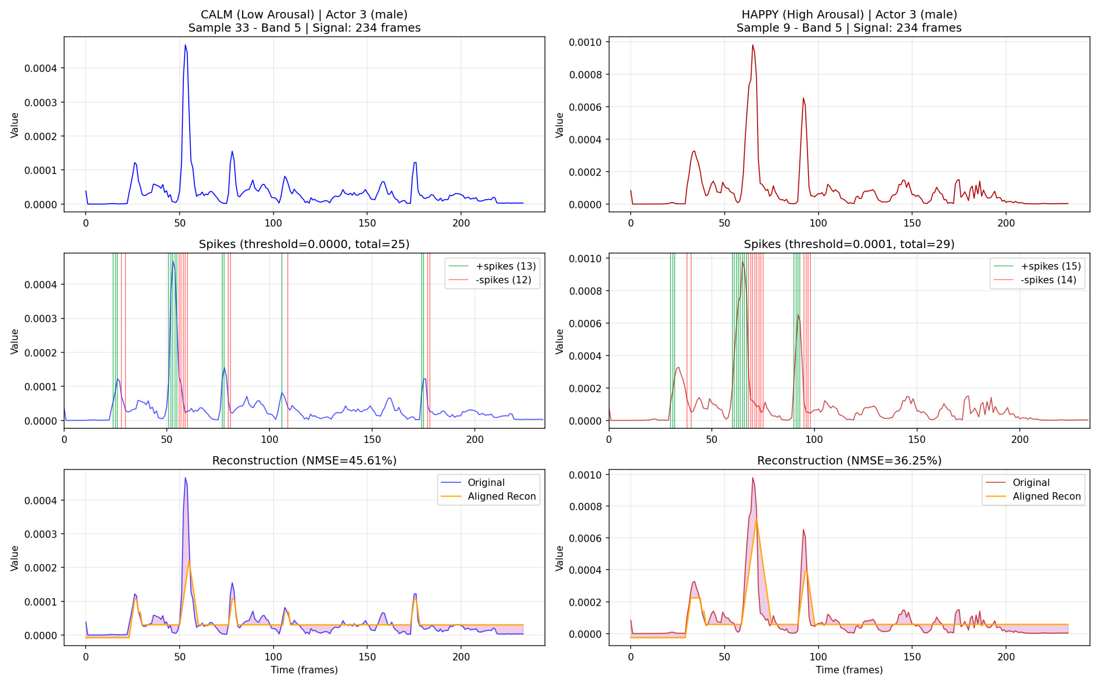
Figure A.2.
Mapping of linear_fft features into the SNNcube.
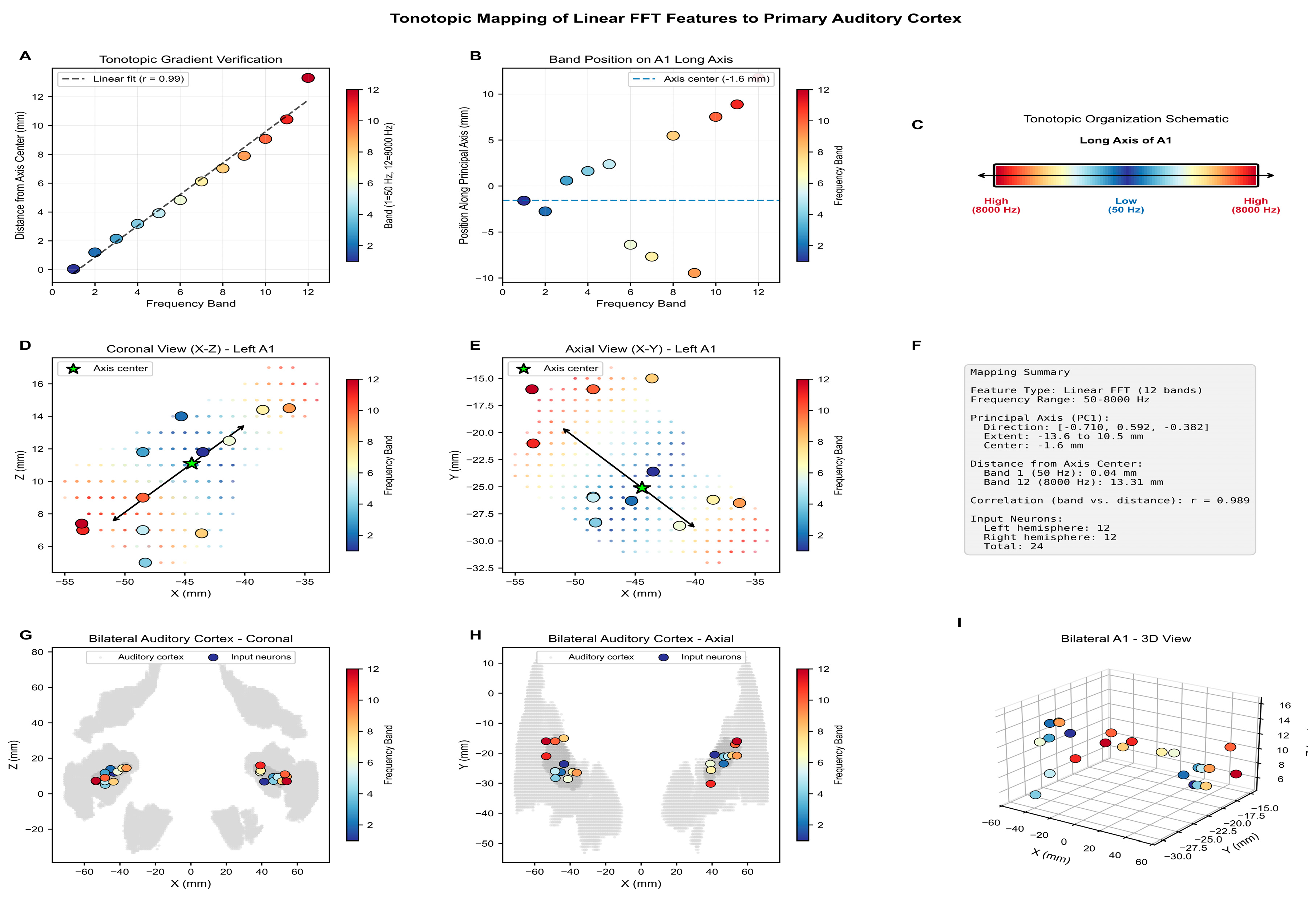
A.2 Experimental Details of the Tonotopic Mapping of Audio Features into the SNNcube
- The following setup was used for the tonotopic mapping of audio features:
- The HCP-MMP1 atlas (Glasser et al., 2016) on MNI152 template was used.
- A hybrid downsampling scheme was applied: 2.5 mm resolution for the auditory cortex and 8.1 mm for the rest of the brain, resulting in 4176 neurons in total (840 auditory + 3336 other neurons).
- Input neurons were placed only in A1 (primary auditory cortex) in both hemispheres.
- A PCA-based gradient was used to distribute neurons evenly along the tonotopic axis (high → low → high frequencies).
- A direct 1:1 mapping was applied: sample column i → neuron i
The HCP-MMP1 atlas provides precise anatomical boundaries for auditory regions:
- A1 (Core): Primary auditory cortex with sharp frequency tuning and direct sensory input.
- Belt: Surrounding A1, integrates frequency channels and supports phonemes/timbre processing
- Parabelt: Higher-level auditory processing, including speech and music categories.
Features were mapped specifically to the A1 region of the SNNcube for the fol-lowing reasons:
- Biological plausibility: Mimics how the real auditory cortex receives input.
- Spatial learning: Enables the SNN to learn spatial relationships between frequency bands.
- Interpretability: Neuron activations correspond to known brain regions.
- Emergent organization: As shown in TopoAudio (29), spatially constrained networks can develop brain-like organization without explicit supervision.
With this mapping, the following behavior is observed:
- Only A1 (core) receives direct input, not belt or parabelt regions.
- A1 neurons are frequency-selective, similar to mel spectrogram or fft bands.
- Belt regions receive processed output from A1 via learned SNN connections.
- Parabelt regions receive output from belt regions.
- This mapping matches the biological processing hierarchy.
From the HCP-MMP1 atlas on MNI152 template, the hybrid downsampling is applied as follows:
- Auditory cortex: 2.5 mm voxel size (high resolution for input neurons).
- Other regions: 8.1 mm voxel size (standard NeuCube resolution).
- Result: 840 auditory neurons + 3336 other neurons = 4176 total neurons.
A.3. Experimental Details of the Training/Testing Parameters of the eXCube2 Models
The following parameters were used for the three experiments: audio-only, visual-only, and multimodal audio-visual:
Initial dataset (before oversampling):
- Training: 360 samples (6 actors × 60 recordings)
- Testing: 120 samples (2 actors × 60 recordings)
Class imbalance in training data:
- Low arousal (neutral, calm, sad): 120 samples
- High arousal (happy, angry, fearful, disgust, surprised): 240 samples
- Ratio: 1:2 (imbalanced)
After oversampling (training only):
- Low arousal: 240 samples (duplicated from 120)
- High arousal: 240 samples (unchanged)
- Total training set: 480 samples (balanced 1:1)
Test set (unchanged distribution):
- 40 low arousal + 80 high arousal = 120 samples
Signal duration:
- 234–501 timesteps after silence trimming
- Shortest: 234 timesteps × 10 ms = 2.34 s
- Longest: 501 timesteps × 10 ms = 5.01 s
Feature extraction parameters:
- 10 ms hop size, 25 ms window length (standard in speech processing)
Full dataset split:
- Training: 1520 samples (760 class 0, 760 class 1), 19 actors (3–12, 15–23)
- Testing: 1820 samples (860 class 0, 960 class 1), 5 actors (1, 2, 13, 14, 24)
References
- Chern, I.C.; Hung, K.H.; Chen, Y.T.; Hussain, T.; Gogate, M.; Hussain, A.; Tsao, Y.; Hou, J.C. Audio-visual speech enhancement and separation by utilizing multi-modal self-supervised embeddings. In Proceedings of the IEEE International Conference on Acoustics, Speech, and Signal Processing Workshops (ICASSPW), 2023; pp. 1–5. [Google Scholar]
- Saraceno, G. Deep Learning and Memorizing of Spectro-Temporal Data (Music) in the Spatio-Temporal Brain. Master’s Thesis, University of Trento, Trento, Italy, 2017. [Google Scholar]
- Zhang, H.; Zhang, B.; Huang, W.; Tian, Q. Gabor wavelet associative memory for face recognition. IEEE Trans. Neural Netw. 2005, 16, 275–278. [Google Scholar] [CrossRef]
- Liu, W.; Quan, Y.; Liu, Y.; Yan, D.-M. Bi-directional modality fusion network for audio-visual event localization. In Proceedings of the IEEE International Conference on Acoustics, Speech and Signal Processing (ICASSP), 2022; pp. 4868–4872. [Google Scholar]
- Lacheze, L.; Guo, Y.; Benosman, R.; Gas, B.; Couverture, C. Audio/video fusion for objects recognition. In Proceedings of the IEEE/RSJ International Conference on Intelligent Robots and Systems, 2009; pp. 652–657. [Google Scholar]
- Su, R.; Wang, L.; Liu, X. Multimodal learning using 3D audio-visual data for audio-visual speech recognition. In Proceedings of the International Conference on Asian Language Processing (IALP), 2017; pp. 40–43. [Google Scholar]
- Zheng, X.; Wei, Y. Audio-visual event and sound source localization based on spatial-channel feature fusion. In Proceedings of the International Conference on Signal and Image Processing (ICSIP), 2022; pp. 106–110. [Google Scholar]
- Kasabov, N.; Postma, E.; van den Herik, J. AVIS: A connectionist-based framework for integrated auditory and visual information processing. Inf. Sci. 2000, 123, 127–148. [Google Scholar] [CrossRef]
- Wysoski, S.G.; Benuskova, L.; Kasabov, N. Evolving spiking neural networks for audiovisual information processing. Neural Netw. 2010, 23, 819–835. [Google Scholar] [CrossRef]
- Beal, M.; Jojic, N.; Attias, H. A graphical model for audiovisual object tracking. IEEE Trans. Pattern Anal. Mach. Intell. 2003, 25, 828–836. [Google Scholar] [CrossRef]
- Yue, Q.; Wu, X.; Gao, J. Audio-visual event localization based on cross-modal interacting guidance. In Proceedings of the IEEE International Conference on Artificial Intelligence and Knowledge Engineering (AIKE), 2021; pp. 104–107. [Google Scholar]
- Chakraborty, S.; Aich, S.; Joo, M.I.; Sain, M.; Kim, H.C. A multichannel convolutional neural network architecture for the detection of the state of mind using physiological signals from wearable devices. J. Healthc. Eng. 2020, 2020, 5467936. [Google Scholar] [CrossRef] [PubMed]
- Chatterjee, D.; Hegde, S.; Thaut, M.H. Neural plasticity: The substratum of music-based interventions in neurorehabilitation. NeuroRehabilitation 2021, 48, 155–166. [Google Scholar] [CrossRef]
- Krautz, A.E.; Langner, J.; Helmhold, F.; Volkening, J.; Hoffmann, A.; Hasler, C. Bridging AI innovation and healthcare: Scalable clinical validation methods for voice biomarkers. Front. Digit. Health 2025, 7, 1575753. [Google Scholar] [CrossRef] [PubMed]
- Rao, A.; Salehi, M.-J.; Vajargah, S.H.; Bourque, J.L. Neural correlates of auditory predictive timing are linked to human vocal pitch stability. Sci. Rep. 2019, 9, 45105. [Google Scholar] [CrossRef]
- Reddy, V. PPINtonus: Early detection of Parkinson’s disease using deep-learning tonal analysis. arXiv 2022, arXiv:2406.02608. [Google Scholar] [CrossRef]
- Kasabov, N. Time-Space, Spiking Neural Networks and Brain-Inspired AI; Springer Nature: Cham, Switzerland, 2019. [Google Scholar]
- Kasabov, N.K. NeuCube: A spiking neural network architecture for mapping, learning and understanding of spatio-temporal brain data. Neural Netw. 2014, 52, 62–76. [Google Scholar] [CrossRef]
- Izhikevich, E.M. Polychronization: Computation with spikes. Neural Comput. 2006, 18, 245–282. [Google Scholar] [CrossRef]
- Abeles, M. Corticonics: Neural Circuits of the Cerebral Cortex; Cambridge University Press: Cambridge, UK, 1991. [Google Scholar]
- Kasabov, N.K. STAM-SNN: Spatio-temporal associative memory in brain-inspired spiking neural networks: Concepts and perspectives. In Recent Advances in Intelligent Engineering; Kovács, L., Haidegger, T., Szakál, A., Eds.; Springer: Cham, Switzerland, 2024; pp. 1–XX. [Google Scholar] [CrossRef]
- Kasabov, N.K. Life-long learning and evolving associative memories in brain-inspired spiking neural networks. MOJ Appl. Bio. Biomech. 2024, 8, 56–57. [Google Scholar] [CrossRef]
- Kasabov, N.K. Spatio-temporal associative memories in brain-inspired spiking neural networks: Concepts and perspectives. TechRxiv 2023. [Google Scholar] [CrossRef]
- Kasabov, N.; Bahrami, H.; Doborjeh, M.; Wang, A. Brain inspired spatio-temporal associative memories for neuroimaging data: EEG and fMRI. Bioengineering Preprints 2023. [Google Scholar] [CrossRef]
- Gao, C.; Green, J.J.; Yang, X.; Oh, S.; Kim, J.; Shinkareva, S.V. Audiovisual integration in the human brain: A coordinate-based meta-analysis. Cereb. Cortex 2023, 33, 5574–5584. [Google Scholar] [CrossRef]
- Kasabov, N. Neucube evospike architecture for spatio-temporal modelling and pattern recognition of brain signals. In Artificial Neural Networks in Pattern Recognition; Mana, N., Schwenker, F., Trentin, E., Eds.; Springer: Berlin, Germany, 2012; pp. 225–243. [Google Scholar] [CrossRef]
- Talairach, J.; Tournoux, P.; Rayport, M. Co-planar stereotaxic atlas of the human brain: 3-dimensional proportional system. J. Laryngol. Otol. 1988, 104, 72–73. [Google Scholar]
- Glasser, M.F.; et al. A multi-modal parcellation of human cerebral cortex. Nature 2016, 536, 171–178. [Google Scholar] [CrossRef] [PubMed]
- Al-Tahan, H.; et al. End-to-end topographic auditory models replicate signatures of human auditory cortex. arXiv 2025, arXiv:2509.24039. [Google Scholar]
- Moerel, M.; et al. An anatomical and functional topography of human auditory cortical areas. Front. Neurosci. 2014, 8, 225. [Google Scholar] [CrossRef]
- Kasabov, N.K.; Dhoble, K.; Nuntalid, N.; Indiveri, G. Dynamic evolving spiking neural networks for online spatio- and spectro-temporal pattern recognition. Neural Netw. 2013, 41, 188–201. [Google Scholar] [CrossRef]
- Kumarasinghe, K.; Kasabov, N.; Taylor, D. Deep learning and deep knowledge representation in spiking neural networks for brain–computer interfaces. Neural Netw. 2020, 121, 169–185. [Google Scholar] [CrossRef]
- Kasabov, N.K.; Tan, Y.; Doborjeh, M.; Tu, E.; Yang, J.; Goh, W.; Lee, J. Transfer learning of fuzzy spatio-temporal rules in the NeuCube brain-inspired spiking neural network. IEEE Trans. Fuzzy Syst. 2023, 31, 4542–4552. [Google Scholar] [CrossRef]
- Swanson, R.; Livingstone, S.R.; Russo, F.A. RAVDESS facial landmark tracking (Version 1.0.0) [Data set]. Zenodo 2019. [Google Scholar] [CrossRef]
- Livingstone, S.R.; Russo, F.A. The Ryerson audio-visual database of emotional speech and song (RAVDESS). PLoS ONE 2018, 13, e0196391. [Google Scholar] [CrossRef]
- Cao, F.; Vogel, A.P.; Gharahkhani, P.; Rentería, M.E. Speech and language biomarkers for Parkinson’s disease prediction. npj Parkinsons Dis. 2025, 11, 57. [Google Scholar] [CrossRef]
- Tan, C.; Šarlija, M.; Kasabov, N. Spiking neural networks: Background, recent development and the NeuCube architecture. Neural Process. Lett. 2020, 52, 1675–1701. [Google Scholar] [CrossRef]
- Chen, C.; Al-Halah, Z.; Grauman, K. Semantic audio-visual navigation. 2021. [Google Scholar]
- Guo, L.; et al. Transformer-based spiking neural networks for multimodal audiovisual classification. IEEE Trans. Cogn. Dev. Syst. 2024, 16, 1077–1086. [Google Scholar] [CrossRef]
- Furber, S.B.; Brown, G.; Bose, J.; Cumpstey, J.M.; Marshall, P.; Shapiro, J.L. Sparse distributed memory using rank-order neural codes. IEEE Trans. Neural Netw. 2007, 18, 648–659. [Google Scholar] [CrossRef]
- Behrenbeck, J.; Tayeb, Z.; Bhiri, C.; Richter, C.; Rhodes, O.; Kasabov, N.; Espinosa-Ramos, J.; Furber, S.; Cheng, G.; Conradt, J. Classification and regression of spatio-temporal signals using NeuCube. J. Neural Eng. 2019, 16, 026019. [Google Scholar] [CrossRef] [PubMed]
- James, R.; Garside, J.; Hopkins, M.; Plana, L.A.; Temple, S.; Davidson, S.; Furber, S. Parallel distribution of an inner hair cell and auditory nerve model. In Proceedings of the IEEE BioCAS, 2017; pp. 1–4. [Google Scholar]
- Furber, S.B.; Galluppi, F.; Temple, S.; Plana, L.A. The SpiNNaker project. Proc. IEEE 2014, 102, 652–665. [Google Scholar] [CrossRef]
- Paulun, L.; Wendt, A.; Kasabov, N.K. A retinotopic spiking neural network system for accurate recognition of moving objects. Front. Comput. Neurosci. 2018, 12, 1–15. [Google Scholar] [CrossRef]
- Song, Q.; Kasabov, N. NFI: A neuro-fuzzy inference method for transductive reasoning. IEEE Trans. Fuzzy Syst. 2005, 13, 799–808. [Google Scholar] [CrossRef]
- AbouHassan, I.; Kasabov, N. NeuDen: A framework for the integration of neuromorphic evolving spiking neural networks. Evolving Syst. 2025, 16, 3. [Google Scholar] [CrossRef]
- Kumarasinghe, K.; Kasabov, N.; Taylor, D. Brain-inspired spiking neural networks for decoding muscle activity. Sci. Rep. 2021, 11, 2486. [Google Scholar] [CrossRef]
- AbouHassan, I.; Kasabov, N.; Bankar, T.; Garg, R.; Bhattacharya, B. ePAMeT: Evolving predictive associative memory for time series. Evolving Syst. 2025, 16, 6. [Google Scholar] [CrossRef]
- Gong, Y.; Chung, Y.-A.; Glass, J. AST: Audio spectrogram transformer. arXiv 2021, arXiv:2104.01778. [Google Scholar] [CrossRef]
- NeuCubePy. Available online: https://github.com/KEDRI-AUT/NeuCube-Py.
- Kasabov, N. Global, local and personalised modelling and profile discovery in Bioinformatics: An integrated approach. Pattern Recognition Letters 2007, Vol. 28(Issue 6), 673–685. [Google Scholar] [CrossRef]
Figure 1.
The NeuCube architecture (adapted with modification from [18]).
Figure 1.
The NeuCube architecture (adapted with modification from [18]).
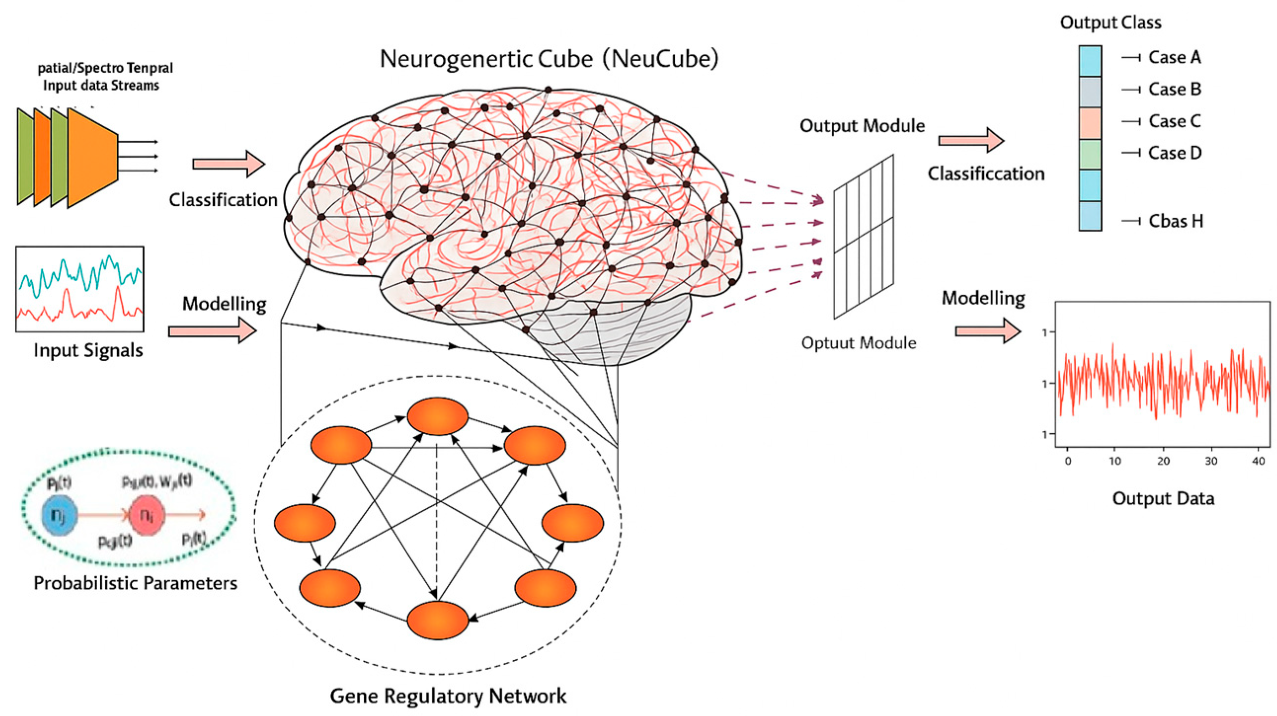
Figure 2.
The problem of detecting a spatio- and spectro-temporal pattern from speech, image, or both modalities, is represented as a classification problem.
Figure 2.
The problem of detecting a spatio- and spectro-temporal pattern from speech, image, or both modalities, is represented as a classification problem.

Figure 3.
The eXCube2 architecture using a brain template for the SNNcube, tonotopic mapping of audio signals and topographic mapping of images for the realisation of the functional diagram from Figure 2.
Figure 3.
The eXCube2 architecture using a brain template for the SNNcube, tonotopic mapping of audio signals and topographic mapping of images for the realisation of the functional diagram from Figure 2.
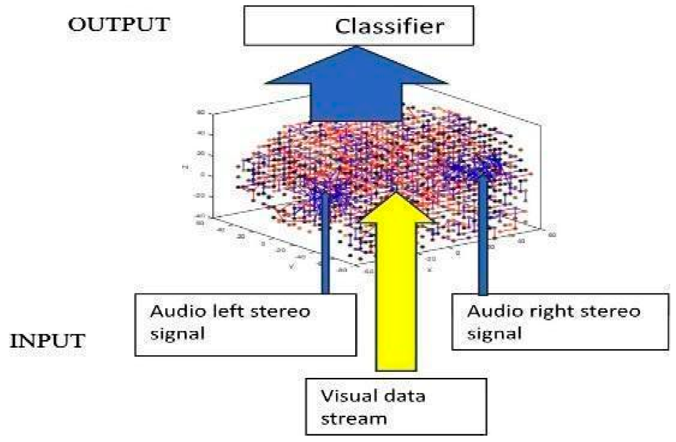
Figure 4.
Examples of extracted mel_spectrogram features from neutral speech (left) and aroused/happy speech (right).
Figure 4.
Examples of extracted mel_spectrogram features from neutral speech (left) and aroused/happy speech (right).
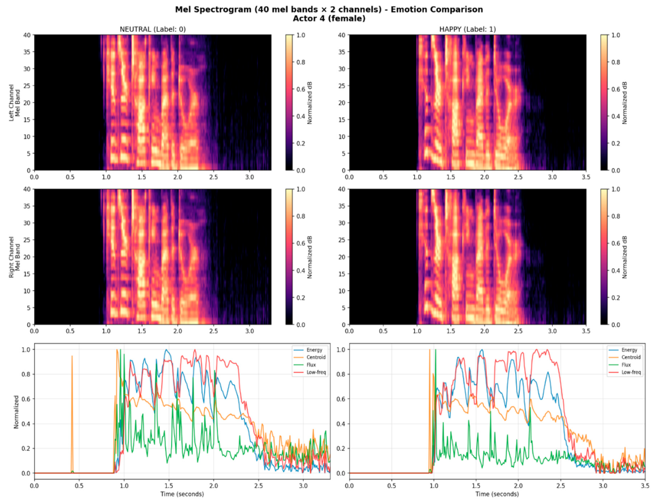
Figure 5.
Spike encoding of the mel_spectrogram audio features from Figure 4 (top) using the Step-Forward method (middle) (see [17]) and reconstructing the signals from the spikes back to the original ones (bottom). It shows that the used encoding method is suitable for the selected features as it results in a small error after reconstruction.
Figure 5.
Spike encoding of the mel_spectrogram audio features from Figure 4 (top) using the Step-Forward method (middle) (see [17]) and reconstructing the signals from the spikes back to the original ones (bottom). It shows that the used encoding method is suitable for the selected features as it results in a small error after reconstruction.
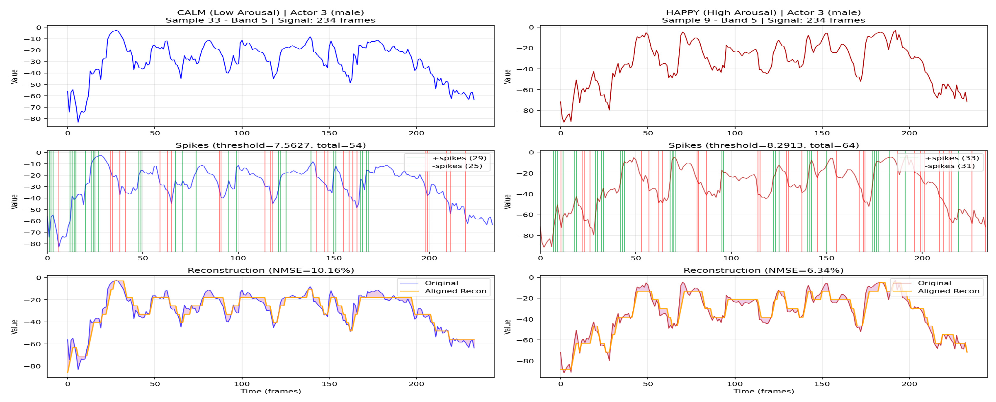
Figure 6.
Mapping of mel_spectrogam features into a 3D SNNcube spatially structured according to the MNI brain template.
Figure 6.
Mapping of mel_spectrogam features into a 3D SNNcube spatially structured according to the MNI brain template.
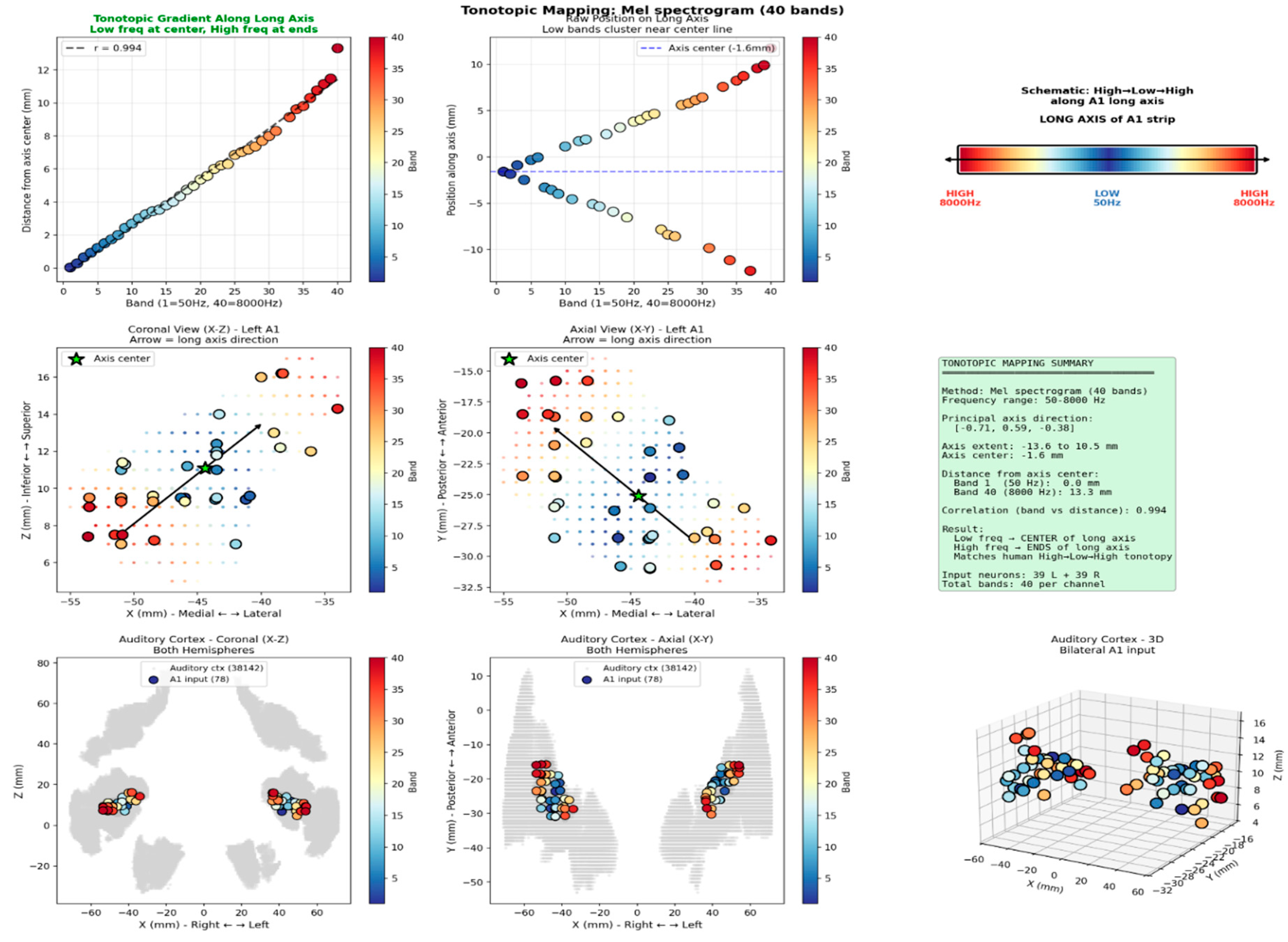
Figure 7.
A snapshot of the activity of the audio (in blue) and visual (in red) features for an exemplar multi-modal data sample in an multimodal eXCube2 model (sample 0 from the data base).
Figure 7.
A snapshot of the activity of the audio (in blue) and visual (in red) features for an exemplar multi-modal data sample in an multimodal eXCube2 model (sample 0 from the data base).
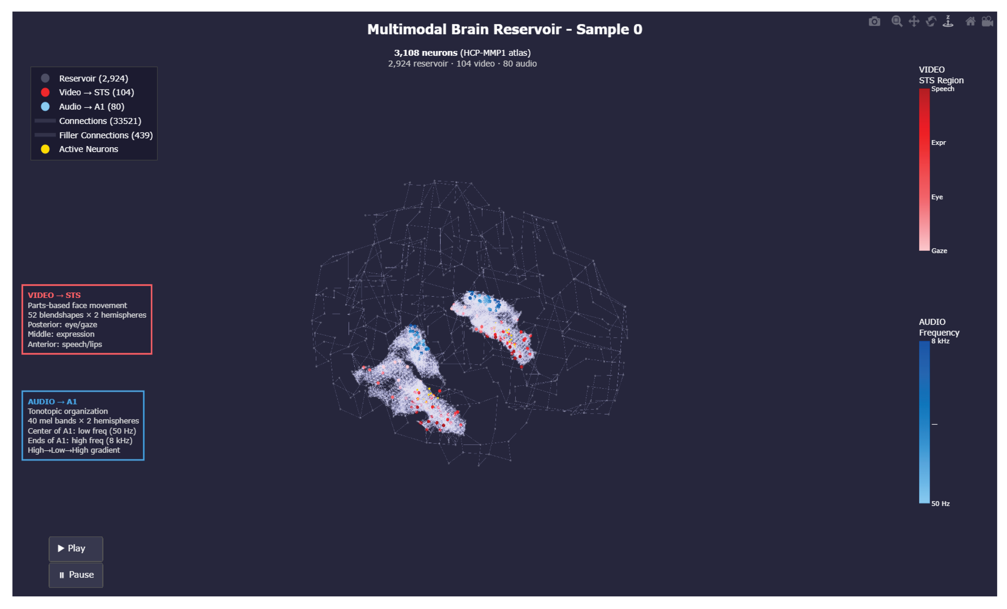
Figure 8.
Visualisation of classification results on multimodal audio-visual data using the multimodal audio-visual eXCube2 model.
Figure 8.
Visualisation of classification results on multimodal audio-visual data using the multimodal audio-visual eXCube2 model.
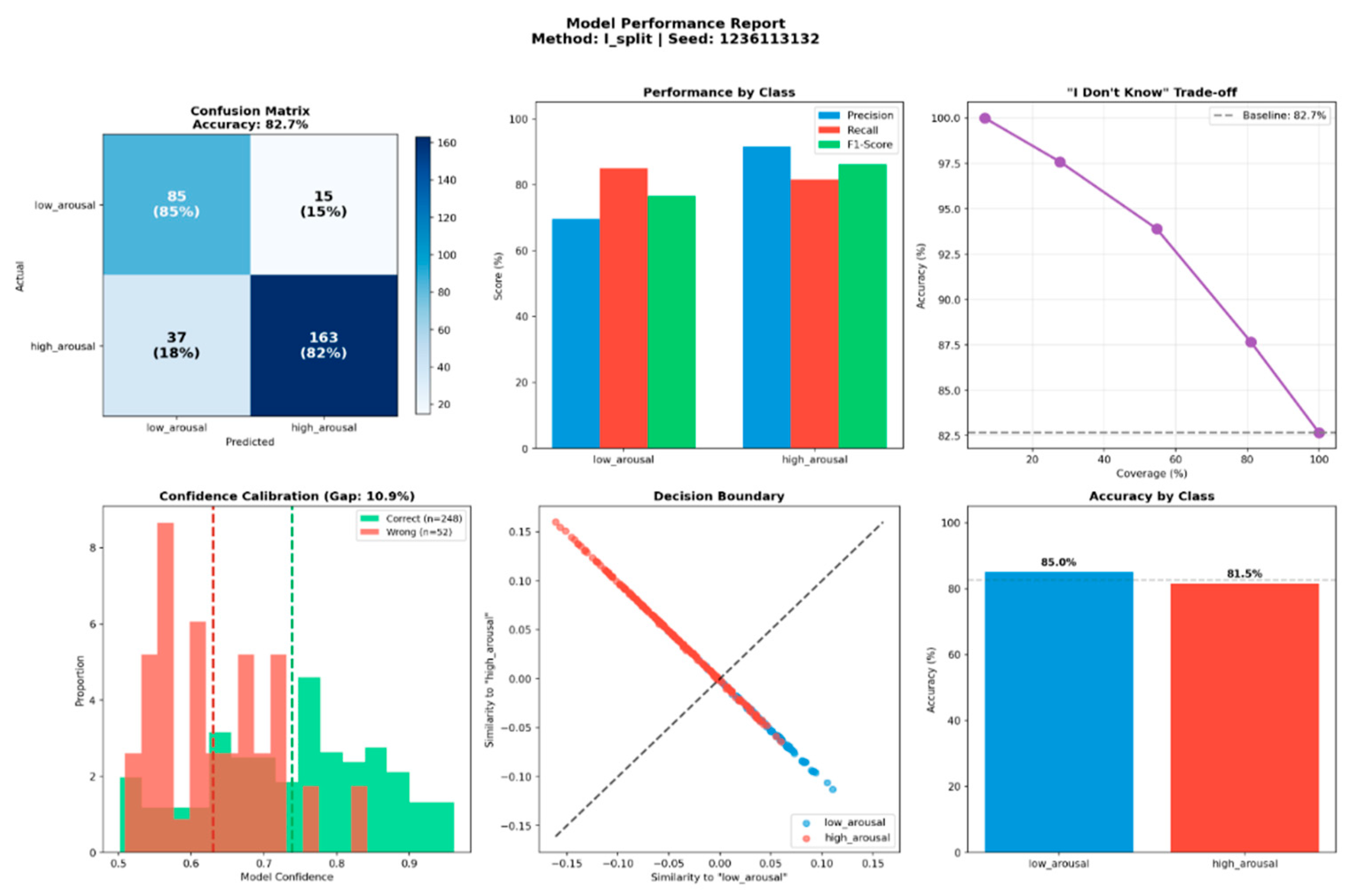
Figure 9.
Visualisation of classification results on audio data using the audio eXCube2 model.
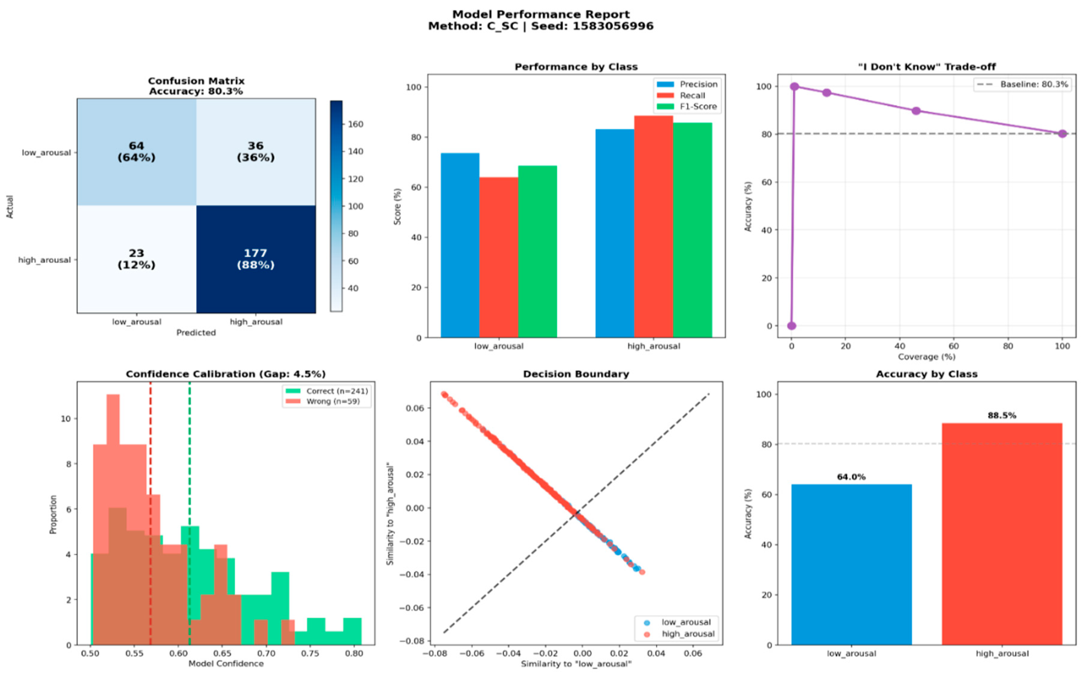
Figure 10.
Visualisation of classification results on visual data using the visual eXCube2 model.
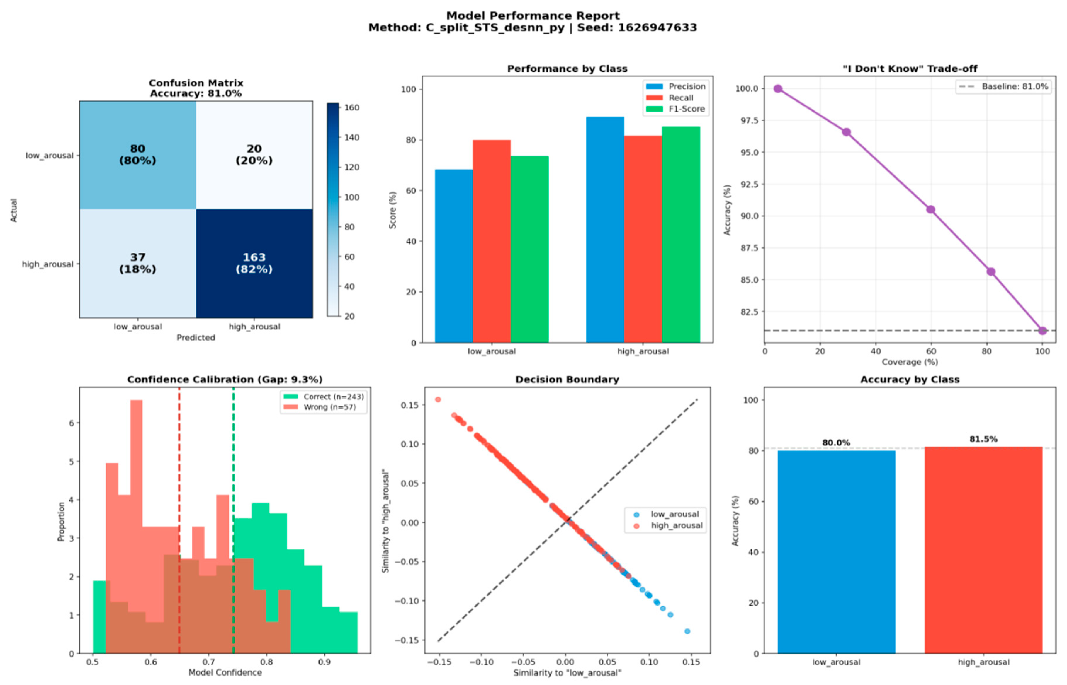
Figure 11.
Spike-time association between 24 linear_fft features (see Appendix A.2 for their mapping into the SNNcube), shown as arcs between features represented as nodes (L means left hemisphere; R means right hemisphere). Thicker arcs indicate a higher number of spikes at the next time step (10 ms) at a node following a spike in its connected node, representing information exchange in spike form.
Figure 11.
Spike-time association between 24 linear_fft features (see Appendix A.2 for their mapping into the SNNcube), shown as arcs between features represented as nodes (L means left hemisphere; R means right hemisphere). Thicker arcs indicate a higher number of spikes at the next time step (10 ms) at a node following a spike in its connected node, representing information exchange in spike form.
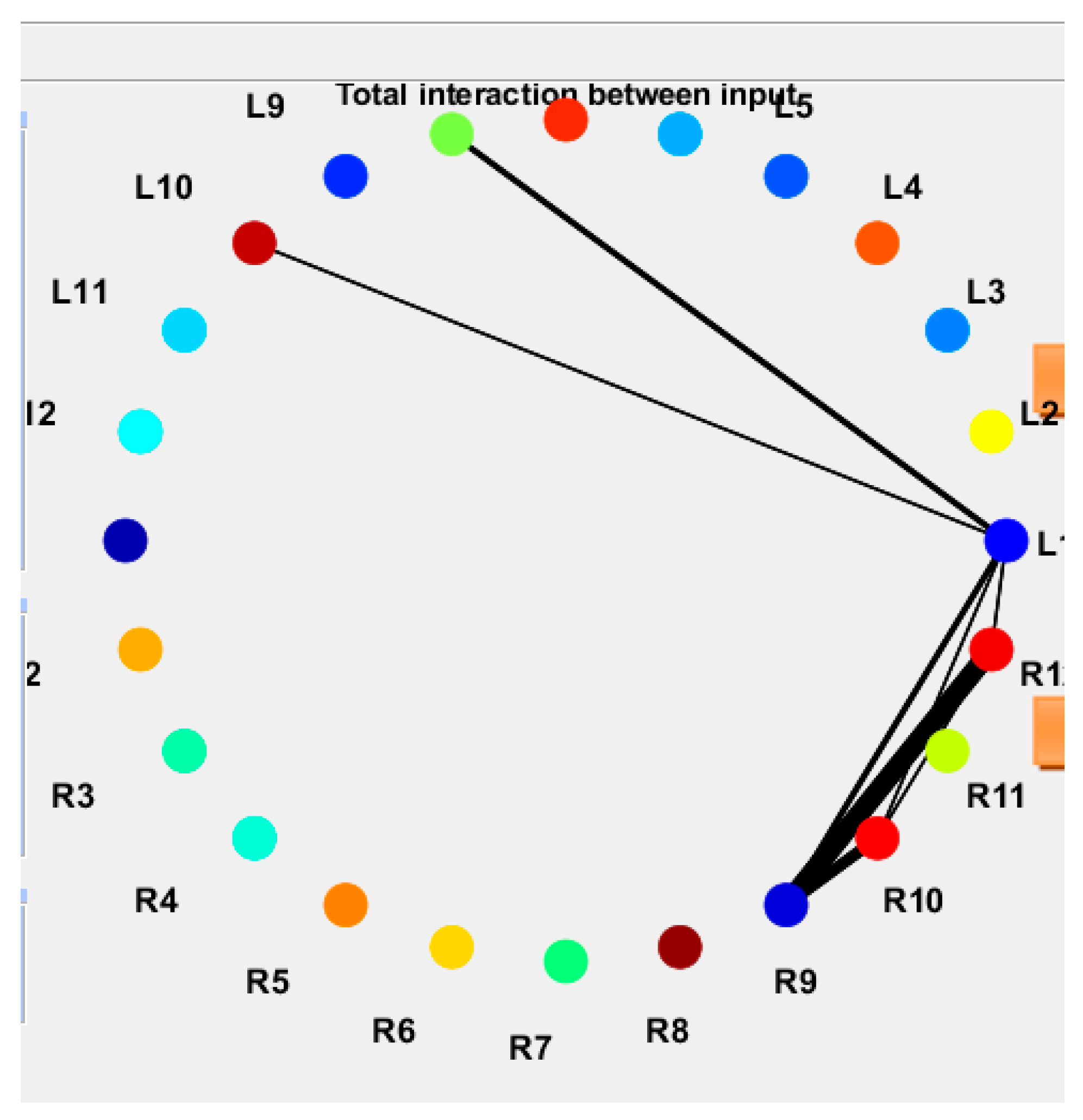

Table 1.
Audio features analysed in this study.
| Feature | Number | Frequencies | In Both Sides | Previous Usage |
| mel_spectrogram | 40 | 50–8000 Hz (mel) | 80 | SOTA emotion recognition |
| mel_fft | 12 | 50–8000 Hz (mel) | 24 | Biologically plausible |
| linear_fft | 12 | 50–8000 Hz (linear) | 24 | Technical analysis |
| mfcc | 12 | Cepstral coefficients | 24 | Speaker-independent ASR |
Table 2.
Algorithm for downsampling and mapping audio features into the SNNcube.
|
For each hemisphere: 1. Extract full-resolution of A1 coordinates of the template (≈858 left, ≈588 right voxels) 2. Identify downsampled neurons within A1 (≈123 left, ≈96 right) 3. Apply PCA to estimate the principal axis of A1 (tonotopic gradient direction) 4. Project neurons onto this axis to obtain a normalised tonotopic position in [0,1] 5. Select neurons evenly spaced along the gradient to match the number of frequency bands 6. Map each audio feature column to one A1 neuron: - Left channel (columns 1 to N) → Left A1 neurons - Right channel (columns N+1 to 2N) → Right A1 neurons 7. Neurons are ordered by tonotopic position, so: - Band 1 (lowest frequency, ≈50 Hz) → maps to the center of A1 - Band N (highest frequency, ≈8000 Hz) → maps to the ends of A1 8. Perform direct mapping where feature column i → neuron i (1-indexed bands), as summarized below: | ||
| Method | Left Channel Mapping | Right Channel Mapping |
| mel_spectrogram | bands 1-40 → neurons 1-40 | bands 1-40 → neurons 41-80 |
| mel_fft | bands 1-12 → neurons 1-12 | bands 1-12 → neurons 13-24 |
| linear_fft | bands 1-12 → neurons 1-12 | bands 1-12 → neurons 13-24 |
| mfcc | bands 1-12 → neurons 1-12 | bands 1-12 → neurons 13-24 |
Table 3.
Audio and visual features and parameters.
| Feature | Audio | Visual |
|---|---|---|
| Features | 80 mel_spectrogram | 52 facial blendshapes |
| Brain region | Bilateral auditory cortex (A1) | Right FFA/STS |
| Input map | Tonotopic (low → high freq) | Topographic |
| Reservoir | 3108 neurons | 3108 neurons |
| Train samples | 160 | 160 |
| Test samples | 120 | 120 |
Table 4.
The used classification methods for the classification of state vectors.
| Method | Mathematical Formulation | Description |
| (a) SVM (RBF Kernel) |
Gamma set automatically. Maximum-margin hyperplane in kernel space. | |
| (b) Weighted Weighted KNN (WWKNN) (Kasabov, 2010)[51] |
Feature-wise SNR weighting, where SNR_f = variance_between(f) / variance_within(f). Downweights noisy features, emphasises discriminative ones. |
|
| (c) Centroid Prototype |
Class represented by a normalised centroid; classification by maximum cosine similarity. | |
| (d) Learned Prototype |
Prototypes optimised via gradient descent on cross-entropy loss. Adam optimiser, lr=0.01, 300 epochs, tau=0.1. |
Table 5.
Accuracy of the three models developed in this study, along with the method used for the state vector extraction.
Table 5.
Accuracy of the three models developed in this study, along with the method used for the state vector extraction.
| Experiment | Method (see the legend below*) | Max Accuracy |
| Multimodal audio-visual | R: STS py | 82.0% |
| I: split | 82.7% | |
| I: hybrid | 82.3% | |
| Audio (mel_spectrograms) | I+R: SC | 80.3% |
| I+R: A1 SC | 80.3% | |
| I+R: A1 hybrid | 79.3% | |
| Video (blendshapes) | I+R: STS hybrid | 80.7% |
| I+R: split STS hybrid | 80.7% | |
| I+R: split STS py | 81.0% |
* Legend:
Table 6.
Comparative accuracy of the eXCube2 models on audio-, visual- and audio-visual data when the “don’t know” output is introduced.
Table 6.
Comparative accuracy of the eXCube2 models on audio-, visual- and audio-visual data when the “don’t know” output is introduced.
| Model | Confidence Threshold | Coverage | Accuracy | Accuracy (with conf. threshold) | Correct | Wrong | Rejected | Lost Correct |
Errors Avoided |
| Video | 65% | 71.3% | 81.0% | 87.9% | 188 | 26 | 86 | 55 | 31 |
| Audio | 55% | 72.3% | 80.3% | 85.3% | 185 | 32 | 83 | 56 | 27 |
| Multimodal | 60% | 81.0% | 82.7% | 87.9% | 213 | 30 | 57 | 35 | 22 |
Disclaimer/Publisher’s Note: The statements, opinions and data contained in all publications are solely those of the individual author(s) and contributor(s) and not of MDPI and/or the editor(s). MDPI and/or the editor(s) disclaim responsibility for any injury to people or property resulting from any ideas, methods, instructions or products referred to in the content. |
© 2026 by the authors. Licensee MDPI, Basel, Switzerland. This article is an open access article distributed under the terms and conditions of the Creative Commons Attribution (CC BY) license (http://creativecommons.org/licenses/by/4.0/).
Copyright: This open access article is published under a Creative Commons CC BY 4.0 license, which permit the free download, distribution, and reuse, provided that the author and preprint are cited in any reuse.