

Submitted:
10 February 2026
Posted:
12 February 2026
You are already at the latest version
Abstract
Unmanned Aerial Vehicle (UAV) imagery has become an important instrument for ero-sion monitoring, but little is known about its application in Mediterranean agricultural systems such as vineyards and olive groves. In this study, drone flights were conducted in vineyards and olive groves where mulch and biochar treatments were applied. Digital terrain models (DTM) and orthomosaics were constructed with a photogrammetry work-flow, and model error was determined through global positioning system (GPS) transects. Erosion was assessed through Digital elevation models of Difference (DoD) and compared with field erosion plot measurements. Explanatory variables for erosion (soil roughness, slope length, steepness, vegetation cover) were derived from the DTMs and orthomosaics and were tested in a multiple linear regression model. Although direct measurement of erosion from the DoDs was limited, this was primarily influenced by the unexpected low erosion rates during the study period, and the high root mean square error (RMSE) in the DTMs. Significant differences in DTM-derived variables were found between study areas, and especially between areas with organic and integrated management, even though treatments showed similar patterns. The multiple linear regression model demonstrated strong explanatory power, accounting for a large part of the variation in measured erosion using the UAV-derived variables (R2 = 0.72). Vegetation cover and slope length were the most important predictors for erosion. The results suggest that soil erosion in the study areas was mostly determined by topographic and management factors, rather than the applied treatments. This study highlights the value of UAV imagery in advancing the un-derstanding of erosion processes in Mediterranean agricultural systems, while it identifies the challenge of accurately measuring erosion from DoDs under conditions of low erosion rates.
Keywords:
photogrammetry
; terrain analysis
; vegetation cover
; erosion modelling
; soil management
1. Introduction
The Mediterranean region stands out as one of Europe’s most sensitive areas to land degradation in [1,2], due to its distinctive arid climate, land abandonment, and unsustainable agricultural practices [3,4]. While soil erosion rates in the Mediterranean are generally lower than in other parts of Europe, this often reflects the already degraded state of soils, underlining that further degradation would have severe impacts [5,6]. Mediterranean erosion rates are generally highest in croplands, where it causes a loss of fertile soil and leads to reduced productivity in agricultural systems [1]. Vineyards and olive groves are the agricultural systems that are most prone to erosion, with vineyards having the highest erosion rates by far [5,7]. The main causes for high erosion rates in these systems are low vegetation cover, tillage, and steep slopes [8]. Soil erosion in olive groves has increased over time due to the intensification of olive production and is a major threat to the sustainability of olive groves [9,10]. Furthermore, conventional management leads to reduced sustainability and yield in vineyards [11]. Meanwhile, increased periods of prolonged drought are expected to lead to an intensification of irrigation in olive groves and vineyards, and in turn, this intensification is causing more soil erosion [12].
As one of the most important drivers behind land degradation in many ecosystems, soil erosion negatively affects soil properties, reduces agricultural productivity and available agricultural land [1,13], and leads to a decrease in organic carbon and nutrients as the soil is lost [14]. Furthermore, soil erosion can lead to negative off-site effects such as decreasing water quality [15]. On the local scale, soil erosion causes agricultural systems to become unsustainable, negatively impacting the resilience of farmer livelihoods [16]. Furthermore, erosion-induced decreases in agricultural productivity are a driver of land abandonment [17]. Land abandonment can exacerbate soil erosion and stimulate rural depopulation, negatively affecting rural economies [18]. In turn, rural depopulation eventually leads to the loss of cultural values and traditions of local communities [19]. As such, the prevention of soil erosion is important for both ecological and socio-economic reasons. These factors show that there is a need for research into measures to reduce soil erosion and increase the sustainability of agricultural orchards in the Mediterranean [20].
Remote sensing is a useful tool for the spatial assessment of soil erosion and its different components and is increasingly being used in soil erosion assessment and monitoring [21]. Satellite remote sensing is often used to estimate erosion parameters such as vegetation cover and to map erosion from catchment to global scale by using the measured parameters in erosion models [1,21,22]. On smaller scales, UAV-based (Unmanned Aerial Vehicles, e.g., drones) remote sensing is a suitable alternative [23]. Whereas satellite remote sensing can only be used to measure erosion parameters, UAV-based remote sensing can directly measure soil erosion over time [24]. Furthermore, UAV-based remote sensing can assess soil erosion at a much higher resolution and can calculate soil erosion at a higher accuracy [25] and allows for the accurate assessment of microtopology [26].
UAV-based remote sensing is increasingly used to investigate the components of soil erosion on the field and catchment scale. For example, UAV-based remote sensing has been used to study spatial patterns of erosion [27], calculate sediment budgets [28], detect rill formation in agricultural fields [29], and estimate micro-topological soil parameters such as soil roughness [30]. However, for even smaller scales, such as small erosion plots within fields, UAV-based remote sensing has only been applied in a small number of studies [25], making it relevant to study the use of UAV-based remote sensing on smaller scales.
Many studies have already used field experiments to study soil erosion with conventional methods, such as sediment traps or rainfall simulations [5,31]. However, these methods often do not identify the individual components of inter-rill, rill, and gully erosion and cannot be used to study spatial patterns of sedimentation and deposition. This causes uncertainty about the actual impacts of soil erosion and the influence of different erosion processes, such as the beforementioned rill or gully erosion [32]. Meanwhile, exact measurements of surface changes with high temporal and spatial resolution are needed to investigate the development of erosion patterns over time, which is necessary to understand rill and inter-rill erosion processes [24].
UAV remote sensing can offer new methods for studying soil erosion at the plot scale [24,29,33,34]. Previous research includes only a limited number of studies using UAV remote sensing to assess soil erosion in vineyards [35], and none have focused on olive orchards. Moreover, few studies have compared the effects of different soil conservation measures between plots using UAV remote sensing [36,37], and none have tested the application of biochar; a product that, beyond its effects to reduce erosion, can also improve soil habitat and crop growth [38,39].
To address these research gaps, the present study focusses on vineyards and olive orchards in Alentejo, Portugal, a region where climate change and agricultural intensification have been shown to increase erosion risks [40], making the region an interesting location for studies of soil erosion in Mediterranean agricultural systems. The general objective of this research is to evaluate the applicability and limitations of UAV-based photogrammetry for soil erosion assessment in Mediterranean vineyards and olive groves.
Specifically, this study aims to: (i) assess the accuracy of UAV-derived DTMs and their suitability for quantifying soil erosion through DoDs, (ii) compare erosion estimates derived from DoDs with in-field erosion measurements at the plot scale, (iii) evaluate the effects of mulch and mulch–biochar treatments on soil erosion, and (iv) identify key topographic and vegetation-related variables derived from UAV data that explain spatial variability in measured soil erosion. By addressing these objectives, this study provides insight into both the potential and the current limitations of UAV photogrammetry for erosion monitoring in Mediterranean agricultural orchards.
2. Materials and Methods
2.1. Study Area and Experimental Design
This research was conducted across four study areas in Portugal’s Alentejo region: two olive orchards and two vineyards. The olive orchards were the irrigated, integrated-management Vale Formoso (VFO) area near Granja (40 km east of Évora, GPS coordinates 38°18′13.3”N 7°16′37.6”W) and the organic, rainfed Mouchão Olive (MOO) area near Casa Branca (20 km north of Évora, 38°55′03″ N 7°47′20″ W). Approximately 600 m from MOO lies the integrated-management Mouchão Vineyard (MOV) area, with the second vineyard, the Fundação Eugenio de Almeida (FEA) area, situated 15 km east of Évora (38°31′03″ N 7°44′17″ W). In the integrated-management study areas, ground cover was permitted to grow throughout, with herbicide application focused near the tree lines [10,41]. The regional climate is characterized as hot-summer Mediterranean (Köppen Csa), with a mean annual temperature of 16 °C and annual precipitation ranging from 500 to 600 mm. Soil parent materials were slate/conglomerate at VFO, conglomerate at MOO and MOV, and schist at FEA. Soils were classified as Cambisols, except for Regosols and Luvisols identified at the MOO and MOV areas. Nine erosion plots with areas ranging between 150 and 200 m2 were set up in each study area, in three blocks of three plots each. Three different treatments were randomly applied to each of the plots: untreated, a mulch layer, and a mulch layer over a biochar layer applied previously. The mulch application rates were 3 Mg/ha of olive leaves in the olive groves and 2 Mg/ha of straw in the vineyards. Biochar was applied at a rate of 10 Mg/ha in both land uses. The treatments were applied in a completely randomized block design, with three blocks of three plots per location, resulting in 36 plots. Figure 1 shows a map with the locations of the study sites, and Table 1 shows a summary of the plots and treatments per study area.
2.2. In-Field Erosion and Bulk Density Measurements
Sediment fences [42] were installed at the downslope end of every erosion plot. Sediment was removed from the fences and weighed during monthly field visits. The dry weight of the sediments was determined by drying sediment samples in the lab.
Soil bulk density of each plot was determined to calculate the weight of eroded sediment estimated with the DoDs. Per plot, nine soil samples were taken: in the bottom, middle, and top of the plot, and for three micro-environments: below the tree or vine, in areas compacted by wheel passages, and in vegetated areas. All samples were weighed and then dried for 24 hours at 105 degrees Celsius. After drying, the samples were once again weighed. The bulk density was calculated as the mass of dry soil divided by the total volume of the sample.
2.3. Deriviation of Digital Elevation Models
Two sets of drone flights were conducted, in early November 2024 and in early April 2025. A Mavic 2 Pro Camera was used, with a resolution of 0.8 cm per pixel. DTMs were created from the photographs of each drone flight through a Structure from Motion photogrammetry workflow, using the Agisoft Metashape Pro software [43]. Ground Control Points (GCPs) were used to geo-reference the DTMs. Geo-referencing was necessary to correct camera calibration parameters in the Metashape software and to remove deformations in the sparse point cloud [44,45]. Coregistration was used to align the 2025 DTMs with the 2024 DTMs. Coregistration is a technique used for multitemporal topographic datasets, where the second DTM is aligned with the first DTM by identifying areas where no elevation change has taken place (e.g., rocks, roads) and using these areas as GCPs in the second DTM [44,46]. A Trimble Catalyst GPS was used to record the x, y, and z coordinates of the GCPs and several transects within the erosion plots with an average accuracy of 0.01 meters. In total, 12 transects were surveyed, one for each block of plots. As a measure of DTM model error, the Root Mean Square Error (RMSE) between the elevation of GPS points and the elevation of corresponding points in the DTMs was calculated, where the GPS data was used as ground truth data. Table 3 presents an overview of the drone and GPS surveys per study site.
2.4. Erosion Estimation from DTMs
DEMs of Difference (DoD) were calculated for each plot to estimate the erosion between the 2024 and 2025 drone flights. DoDs were calculated by subtracting the 2025 DTMs from the 2024 DTMs. The error propagation to the DoD was calculated as shown in formula 1 [47,48,49]. A “level of detail” (LoD) is used to include the DoD error in the erosion estimation. The LoD can be seen as a confidence interval for the change in elevation between the first and second DTM, where only elevation changes outside the confidence interval will be seen as actual topographic changes. Previous studies show that a 95% LoD is generally appropriate (formula 2) [47,50].
where is the propagate error, the error from the respective DTM, and the 95% Level of Detail. The net eroded volume was calculated as the sum of all significant elevation differences in the DoD times the raster cell size. This volume was converted into eroded weight by multiplying by the plot average bulk density.
2.5. Deriviation of Topographic Variables
Several variables were derived from the DTMs and orthomosaics, including plot area, length, and slope, as well as surface roughness and vegetation cover.
For the surface roughness calculations, the DTMs were first detrended to remove global effects such as slope that could affect the roughness calculations [24]. DTMs were detrended by fitting a linear, first-order polynomial to the DTM, and subtracting this polynomial from the original DTM. The Root Mean Squared Height (RMSH), also called the Random Roughness Index (RR) was calculated to quantify surface roughness [51].
where z is the elevation in one cell, the average elevation, and n the number of cells. Vegetation cover was derived from the orthomosaics using the VARI index, vegetation index that only uses the red, green, and blue wavelength bands, and does not require near-infrared data [52].
where equals the reflectance of the respective wavelength band. A threshold was used to determine vegetated areas from the resulting VARI index maps. All cells with a value above the threshold were classified as vegetation and below as bare soil. The threshold was selected by visual inspection of several threshold options in comparison with the original orthomosaics. The threshold differed slightly between the 2024 and 2025 drone flights and between areas but was generally between 0 and 0.1. The VARI maps were classified into vegetation and bare soil, and the vegetation cover was calculated as the percentage of vegetation cells divided by the total amount of cells per plot.
2.6. Statistical Analysis
All statistical analyses were performed in the R environment using the RStudio package. The accuracy of the net erosion estimates was assessed by calculating the RMSE and R2 metrics. The RMSE is a measure of model accuracy, with a lower RMSE meaning a more accurate estimation of erosion compared to the ground truth. The coefficient of determination (R2) is a measure of the goodness of fit for a model compared to the ground truth, with a higher value meaning a better fit.
Relative error in field measurements of sediment weights from erosion plots becomes larger as the actual weight of sediments in the sediment traps becomes smaller. In cases of very low erosion rates, this can significantly affect the accuracy assessment of erosion model estimations [53]. Nearing (2000) defined occurrence intervals between which the relative difference between actual and predicted erosion is deemed acceptable for different erosion rates [54]. The occurrence interval’s upper and lower boundaries of the occurrence interval are defined with the following equations:
As the erosion rates in some plots were very low during this study, Nearing’s effectiveness coefficient was calculated as an extra accuracy metric, as this metric can give a fairer assessment of model accuracy at very low erosion rates. The effectiveness coefficient is defined as the percentage of model predictions of which the relative difference with the field measurements falls within the 95% occurrence interval:
The effects of the different treatments on measured erosion, soil roughness and vegetation cover parameters were statistically analyzed using one-way ANOVA, where the treatments and study area locations were the qualitative predictors. Logarithmic transformation of the data was performed in case the normality assumption was violated, which was checked with the Shapiro-Wilk test. If the ANOVA resulted in a significant outcome for the F-test, treatments were compared pairwise using Tukey’s procedure for pairwise comparisons.
A multiple linear regression was performed to investigate if the UAV-derived variables could be used to explain the erosion measured in the field. First, a correlation analysis was performed to identify variables that could be used in multiple linear regression. As several variables were not normally distributed, Spearman’s (non-parametric) rank correlation coefficient was calculated. Variables that had a significant correlation with the measured erosion were selected.
3. Results
3.1. DTM Accuracy Assessment
Table 4 shows summary statistics for the 2025 DTMs. The DTM resolution was lower than 0.02 meters for all areas. The number of coregistration points varied per area and was mainly dependent on the number of stable points that could be found between the 2024 and 2025 drone images. In general, RMSE and 95% LoD were higher in olive groves. The MOV1 and MOV2 areas were located next to each other, and both areas were surveyed in one continuous drone flight, resulting in one DTM containing both areas. However, separate GPS transects were surveyed for each area. This explains why the resolution and number of coregistration points are equal between MOV1 and MOV2, but the RMSE and 95% LoD differ.
Figure 2 shows graphs of the GPS transects per DTM, with the heights of the transect points on the y-axis and the distance along the transect on the x-axis. The blue line shows the corresponding height values of the DTMs along the transect. From Figure 2 it is visible that in the vineyards (FEA and MOV), and VFO, there was generally a good fit between GPS and DTM. The MOO DTMs had a much higher RMSE compared to the other areas, and Figure 2 shows that the GPS transects did not fit as well with the DTMs. For the 2025 MOO1 area, it was not possible to generate a correct DTM, explaining the misalignment with the GPS transect and the high RMSE.
Figure 3 compares both methods and their accuracy compared to the GPS transects. In general, the two methods performed similarly and the differences between the transects were small. In VFO3, the coregistration method performed much better, and Figure 3 shows that the transect line of the geo-referencing method follows a similar shape as the GPS and coregistration transects, however, there is a systematic difference in elevation between the GPS and geo-referencing lines.
3.3. Erosion Estimation from DTMs
Figure 4a shows the erosion predicted by the DoDs against the measured erosion. The DoDs could not accurately predict the erosion in most of the plots. In many of the plots, no erosion was detected at all. The DoDs showed a net deposition due to vegetation growth, which was not successfully filtered. After plots with net deposition were removed from the analysis, the final R2 was 0.1361, and the RMSE was 0.4377. Figure 4b shows the relative difference between the measured and predicted erosion for each plot. Relative differences that fall within the occurrence interval are deemed acceptable differences. The final effectiveness coefficient e was 0.55 for a 95% occurrence interval.
3.4. Patterns in DoD Elevation Changes
Elevation changes caused by agricultural management, external disturbances, and data processing were found to be much greater than changes caused by water-induced erosion. Figure 5 illustrates these changes, showing a selection of DoDs of the erosion plots. Elevation changes caused by agricultural management included compaction in ruts and raised sides of ruts caused by frequent tractor passages. Furthermore, in locations where vegetation was not successfully removed from the DTM, increases due to growth of vegetation strips were visible. Some areas of the plots were not covered by the drone surveys, usually due to high vegetation cover. These areas were interpolated during the creation of the DTMs, which introduced inaccurate elevation changes in the DoDs. Finally, some elevation changes were caused by soil samples taken between the 2024 and 2025 drone surveys.
3.5. Comparison Between Treatments and Areas
Figure 6 shows boxplots of measured erosion, random roughness, and vegetation cover. None of the investigated variables showed significant differences between treatments, but all variables showed significant differences between locations. Table 5 shows the outcomes of each ANOVA including p-values and post-hoc tests.
3.6. Multiple Linear Regression Analysis
Figure 7A shows a correlation matrix containing all correlations between the measured erosion and UAV-derived variables. Significant correlations were found between measured erosion, vegetation cover, and slope. No significant correlations were found between measured erosion, roughness, and plot length. As there was a high rate of collinearity between the 2024 and 2025 vegetation cover, only the initial (2024) vegetation cover was chosen for further analysis.
Figure 7B shows a forest plot displaying the results of the multiple linear regression model that explained the highest proportion of variance, while all predictors were significant. The model had an R2 of 0.72 and an RSE of 0.45. The slope and plot length predictors were not significant on their own, but the interaction between slope and plot length was significant and led to an increase in R2 and a decrease in RSE. Slope was not a significant predictor when added to the regression model. However, when an interaction term with plot length was added, the interaction between slope and plot length became a significant predictor. Model 2 shows that the slope had a regression coefficient of 0.95, and the plot length had a regression coefficient of 0.24. However, due to the interaction term, which had a regression coefficient of -0.02, the effect of each predictor is dependent on the other predictor. For example, a unit increase in slope would cause an increase in measured erosion of 0.95 - 0.02 * slope length.
4. Discussion
4.1. DTM Construction and Accuracy Assessment
All DTMs had a resolution higher than 0.02 meters. These results were similar to previous studies in agricultural orchards, although the resolution is highly dependent on several factors such as flight altitude, camera resolution, and overlap between pictures [55,56]. A comparison of the 2025 DTMs with the GPS transects showed large differences in RMSE between the different study areas. Furthermore, it showed that RMSE values were much lower in vineyards than in olive groves. This was an expected result, as areas where a larger percentage of the ground is obscured by vegetation canopy have been shown to lead to less accurate results for UAV photogrammetry [57,58]. There was a large difference in RMSE values between the two olive orchards, with MOO having much larger values than VFO. This outcome was counterintuitive, as the VFO area has a higher canopy cover and thus was expected to have higher RMSE values. However, this can be explained by the decrease in RMSE as the number of coregistration points decreased. Even so, it was not an obvious outcome that more coregistration points would lead to a lower RMSE, as the 2024 DTMs themselves were models and not true elevation data, and the GPS transects had been surveyed during the 2025 drone flights. However, what separated the 2024 DTMs from the 2025 DTMs was that the 2024 DTMs were directly georeferenced through ground control points, while the 2025 DTMS were indirectly georeferenced through alignment with the 2024 DTMs. This shows that georeferencing is crucial for accurate DTM generation, as was also concluded by previous studies [44,45,58,59]. Furthermore, it suggests that the coregistration process could be enhanced by georeferencing the 2025 DTMs with ground control points, concurrent with the alignment with the 2024 DTMs [60].
Comparing coregistration and georeferencing methods showed that, in general, coregistration did not produce better results than georeferencing. VFO 3 was the exception, as here there was a systematic error in the elevation of the georeferenced DTM. It is possible that this was caused by an error in the georeferencing process, but it could also have been caused by errors during the drone survey. Coregistration of multitemporal DTMs has mostly been used on larger scales [44,46] and is not often used in small-scale agricultural areas. This study did not show that coregistration was beneficial for erosion monitoring. The use of coregistration on a small scale in agricultural fields turned out to be limited, as it was difficult to identify sufficient areas that did not undergo any elevation change. Furthermore, whereas on larger scales, areas such as rocky outcrops can be used as coregistration points [46], coregistration in the study areas had to rely on singular rocks or other small features. It cannot be said with certainty that there was no elevation change in these features. If a coregistration point had an elevation change between the 2024 and 2025 drone flights, it could have introduced an extra error into the model. As such, the placement of permanent ground control points that remain in the study areas for the duration of monitoring could reduce the uncertainty of elevation changes in control points, reduce the error introduced by unknown elevation changes, and improve the accuracy of the DTMs [60,61].
4.2. DTM Erosion Estimation
It was not possible to accurately estimate the soil erosion in the plots, as the estimated erosion only had an R2 of 0.14 compared to the measured erosion. The accuracy in this study was much lower than other studies using a similar approach, although specific R2 values were not reported [62]. The accuracy of the DTMs and error propagation towards the DoDs could be largely held responsible for the low accuracy in erosion estimations. As in most plots, the total measured erosion did not exceed 0.2 tons per hectare; the actual elevation changes in the plots were far below the 95% Level of Detection threshold. This becomes clear when the measured erosion is calculated as depth of topsoil loss. For example, 207 grams of sediment was measured in plot FEA 1. This would equal a depth of 0.011 meters, which is significant as the 95% LoD for this plot was 0.117 meters. Similarly, plot MOV 9 saw 78 grams of erosion, equaling a depth of 0.005 meters which was smaller than the 95% LoD of 0.211 meters. This was also true for plots in the VFO area, where higher erosion rates were measured, but no erosion was found in the DoDs, as the 95% LoD was also larger in this area. This explains why no erosion was found in many of the plots. However, it does not explain why, in some plots, a net deposition was found, despite the plots being closed. Neither does it explain why the erosion of some plots was greatly overestimated.
The net deposition was caused by a combination of outliers in the DTMs and vegetation growth, which has been shown to significantly affect erosion estimates in previous studies [63]. While the filtering of vegetation with the VARI index was able to remove most vegetation, some ground vegetation was not detected and was included in the erosion estimations. If these areas with unfiltered vegetation grew during the study period, they would contribute to the deposition in the DoDs. As erosion rates were low in most plots, even small patches of unfiltered vegetation could cause a net deposition at the plot scale. The plots with greatly overestimated erosion were all found in the VFO study area. Here, a systematic difference between the two DTMs caused the 2025 DTM to be lower than the 2024 DTM, despite the coregistration. It is most likely that this systematic error was caused by the dense canopy and ground vegetation cover during the 2025 flights and ultimately shows the limitations of UAV photogrammetry in densely vegetated areas [57,58].
Another important factor explaining the low accuracy of the soil erosion estimations in this study is the natural seasonality of soil erosion in Mediterranean climates. Several studies have shown that under Mediterranean conditions, soil erosion varies strongly with season, with higher erosion occurring when vegetation cover is low and intense rainfall events occur after prolonged dry periods, and comparatively low erosion rates during wetter seasons with more vegetation cover. For instance, Ferreira and Panagopoulos (2014) used the Revised Universal Soil Loss Equation (RUSLE) approach and found that the highest predicted soil erosion rates occurred in autumn, contributing approximately 65% of the total annual erosion due to reduced vegetation cover after the dry summer, while predicted erosion in winter was much lower (≈ 7% of the total) despite relatively high rainfall erosivity during that season [64]. These findings suggest that the November-April period of the current study may be inherently less erosive in Mediterranean agricultural systems because the soil is wetter and less repellent and vegetation cover typically increases after early autumn rains, reducing the susceptibility of soil to detachment and transport [65].
While the erosion measured in the field was used as ground truth data in this study, it is important to realize that these measurements also contain a degree of error compared to the actual erosion. One source of error in measured erosion could be wind erosion, which can significantly influence soil loss in runoff plots [66]. Errors in sediment sampling, either due to equipment or human error, could also influence the error in the measured erosion [67]. Nearing et al. (1999) stated that there is a high variability in measured erosion for similar plots, and that this variability increases as erosion rates decrease. This variability will also affect the evaluation of soil erosion models [53]. As the acceptable relative difference between estimated and measured erosion becomes larger according to Nearing’s occurrence intervals, many of the relative differences between measured and predicted erosion in this study fell within the 95% occurrence intervals, resulting in an effectiveness coefficient of 0.55. Nearing’s occurrence intervals allow us to determine the performance of erosion estimations while taking this variability into account. As erosion rates become lower, the variability between erosion plots increases, which makes Nearing’s occurrence intervals especially relevant in studies with low erosion rates. This became evident from this study’s erosion estimations, as even though the R2 of the DoD estimations was only 0.14, over half of the estimations could be considered acceptable according to the 95% occurrence intervals. This shows that the smaller the actual erosion is, the harder it becomes to estimate erosion through DoDs or erosion models.
4.3. Comparison Between Treatments and Areas
The analysis showed no significant differences between treatments and control. Application of mulch or mulch with biochar did not affect the measured variables at the time of this study. Previous studies have shown that the effectiveness of mulch and biochar changes over time [68,69,70], although the exact timeframe for which the application is effective is unknown. This could explain why there were no significant differences between treatments in this study. However, most studies on the long-term effects of mulch and biochar were focused on post-fire applications, and no literature for vineyards and olive groves was found, indicating a knowledge gap. As the treatments were applied one year before this study, it cannot be said if they had any effect closer to the time of application.
The ANOVA analysis showed some differences in the measured variables between some of the study areas. For the measured erosion, VFO had significant differences with all other areas, because VFO was the only area where higher erosion rates took place. For the 2024 vegetation cover, MOO had significant differences with all other areas. As MOO was the only organic orchard among the study areas, this explains the difference in vegetation cover, as organic farming has been shown to lead to higher winter vegetation cover in olive orchards compared to non-organic farming [71]. For the 2025 vegetation cover, MOO and VFO were significantly different from FEA and MOV, showing that olive groves generally have a higher vegetation cover [72].
4.4. Multiple Linear Regression Analysis
The multiple linear regression showed that a large amount of variability in measured erosion could be explained by the predictors. Compared to previous studies, the regression model performed similarly or better than comparable models in other studies [73,74,75], but did not perform as well as some studies using more advanced machine learning algorithms [74]. For example, Arnaez et al. (2007) achieved an R2 of 0.74 in vineyards, with other studies achieving similar scores through multiple regression [75]. However, Sahour et al. (2021) showed that it was possible to achieve better results using deep learning (R2 = 0.95) or boosted regression trees (R2 = 0.99) compared to multiple linear regression (R2 = 0.77) [74]. It is important to note that the above-mentioned studies were conducted on a larger scale and time frame, and that no literature was found that used more complex machine learning techniques to investigate erosion for similar areas and time frames to this study.
The plot area was not important for the variation in measured erosion, even though it was a significant predictor in the regression. This is a logical outcome, as the measured erosion in the regression models was given as an erosion rate in tons/ha, so the plot area is already considered in the response variable. It is to be expected that if the response variable were given in total weight, the plot area would be a much more important predictor. In literature, some studies have reported a significant connection between plot area and erosion rates; larger plots could lead to a reduction in measured erosion rates due to more possibilities of sediment deposition within the plot [76,77], or erosion rates could increase due to more erosion processes taking place at larger scales [76]. However, the analysis shows that these factors did not affect erosion rates in this study. Scale effects for differences within the plot scale have been reported for smaller differences than those in this study [78]. The area may become a more relevant predictor for erosion, as the differences in area and subsequent scale effects become larger [79].
Higher initial ground cover led to lower measured erosion, which is in line with previous literature [80,81,82,83,84]. Model 4 confirmed that initial (2024) vegetation cover was an important predictor for erosion, as it shows that a model with just the initial vegetation cover can explain a good part of the variation in measured erosion. Interestingly, the initial groundcover was significant while the 2025 groundcover was not. The ground cover increased between 2024 and 2025 for the VFO study area, where the highest erosion rates were found. The MOO study area, where the least erosion took place, also saw a large increase in ground cover. High 2025 ground cover in both these areas explains why there was no correlation between the 2025 ground cover and measured erosion. Seasonal variations in ground vegetation cover could have played a role, as most of the study period took place during winter, meaning that the winter (2024) ground cover was present during most of the study period [85]. Furthermore, seasonal variations in vegetation cover have been shown to influence erosion rates [86].
As the slope and plot length interaction is comparable to the LS factor of the USLE model, and the ground cover can be seen as the cover management factor C, the regression analysis showed that erosion in the study areas was mostly impacted by the LS and C factors. These findings are in line with previous research, which states that the C and LS factors are the most important for the determination of soil loss potential [87,88]. This also becomes apparent from studies focusing on the Mediterranean [89]. López-Vicente & Navas (2009) state that “the C factor contributed most to variability; the LS and K factors contributed in a similar way” [89]. In this study, bulk density could be seen as a proxy for the erodibility (K) factor, as it has been shown that bulk density can partly explain variations in the K factor [90]. Interestingly, bulk density was not a significant predictor in the regression analysis, suggesting that the erodibility factor did not have a significant impact on erosion. It could be possible that bulk density was not a good proxy for the erodibility factor, as the high stoniness of Mediterranean soils has been shown to have a large impact on the erodibility [91]. The inclusion of the soil stone fraction in the regression analysis could have been a better representative of the K factor, especially considering that the high stoniness of Mediterranean soils is one of the main causes of low erosion rates in the Mediterranean [5,77].
4.5. Limitations
The erosion estimations were most likely influenced by disturbances that were specific to this study, including disturbance through tractor passages and disturbance by soil sampling. The tractor passages that occasionally took place compressed soil in the ruts, and pushing soil sideways caused raising of the edges of the ruts [92,93]. In the VFO area, rills were starting to form in some ruts during one field visit. However, during the next field visit, these rills disappeared due to compression caused by a tractor passage, and as such, the rills were no longer present during the 2025 drone flights and not visible on the 2025 DTMs. The tractor passages had another effect in the MOO area, where the soil was disturbed to such an extent that it was difficult to find any coregistration points. Furthermore, it was not known where and how often tractor passages occurred. In January, some students visited the study areas to collect soil samples for their research. This resulted in several holes per plot, which could have shown up in the 2025 DTMs as erosion and could have affected the erosion estimates.
This study used a Level of Detection threshold to differentiate between real elevation changes and noise. The downside of this methodology is that the smallest changes are discarded as noise, while they could have been actual elevation changes [49]. In this study, this would have limited the erosion estimations as there were mostly low elevation changes due to the low erosion rates. While many studies assume the same error for every cell of a DTM, in reality the error is spatially distributed and is dependent on topographic parameters such as slope and roughness, and data quality parameters such as point density [46]. Wheaton et al. (2010) proposed the use of a fuzzy inference system to make a spatial model of DTM error by using parameters that have been shown to influence the DTM error as inputs and showed that this led to an improvement in sediment budgets. In future studies, it could be beneficial to include spatially distributed errors in the erosion estimation, especially in areas with low erosion rates, to ensure that small, real elevation changes are not discarded as noise [49].
Vegetation cover was a limiting factor in the olive orchards, resulting in high RMSE values. The canopy cover of the olive trees caused the area below the trees to be obscured, which caused holes in the DTM under the trees, even though oblique photographs were added during the DTM generation process. In these areas, photogrammetry is the most suitable technique for DTM generation, and the use of a LIDAR scanner would lead to better results, as LIDAR scanners can penetrate vegetation and have multiple returns [58,94].
The high RMSE values of the DTMs were the factor that ultimately limited the DoD erosion estimations the most. Besides causing higher RMSE values, vegetation cover also limited the results by causing outliers in the DoDs, which further impacted the erosion estimates. The other limitations had less impact on the estimations, as even without disturbances, the erosion estimates would have been poor. If RMSE values had been much lower, disturbances caused by tractor passages and sampling would have had a larger impact on the results, especially since erosion rates were low. While the limitations discussed in this subchapter severely impacted the erosion estimation, they did not have a big impact on the results of the ANOVA analysis or the regression models.
5. Conclusions
This study investigated the use of UAVs for erosion monitoring in Mediterranean agricultural orchards by direct measurement of elevation differences through DTMs of Difference, and through the derivation of explanatory variables for erosion and multiple linear regression. Furthermore, this study investigated the use of coregistration to improve DoD estimates and reduce model error. Additionally, this study used UAV remote sensing to determine the effects of the application of mulch and mulch with biochar on erosion and other variables.
The main conclusions of this study are summarized below:
- Comparison between coregistration and georeferencing methods showed that coregistration did not lead to an improvement in DTM error compared to traditional georeferencing.
- The high RMSE values of the DTMs prevented accurate estimation of erosion with the DoDs, also because of low erosion rates during the study period.
- The ANOVA analysis showed no differences between the control, mulch, and mulch with biochar treatments. Only differences between areas were found, which could mostly be attributed to the type of agriculture and management in the study areas.
- The regression models were able to explain a large part of the variation in measured erosion and showed that the vegetation cover at the start of the rainy season contributed the most to the erosion, together with the slope length and steepness.
Author Contributions
Conceptualization, TP, SP, JCN and AP.; methodology, SPA; software, TP, AP,; validation, TP, AP; formal analysis, TP, AP, SP, JC; investigation, TP, JC, LC, SP; resources, SP, JCN; data curation, TP, JC, AP; writing—original draft preparation, TP, JCN; writing—review and editing, RP, JC, LC, JCN; visualization, TP, AP, SP; supervision, SP, JCN; project administration, SP; funding acquisition, SP. All authors have read and agreed to the published version of the manuscript.
Funding
This research was funded by Portuguese Funds through the PRR under the SOLVIT sub-project (SOLVIT–Vine & Wine Portugal C644866286-00000011) and through FCT under the Project SOLVO (https://www.solvo.uevora.pt; https://doi.org/10.54499/2022.06004.PTDC) and MED–Mediterranean Institute for Agriculture, Environment and Development (https://doi.org/10.54499/UID/05183/2025) and CHANGE–Global Change and Sustainability Institute (https://doi.org/10.54499/LA/P/0121/2020) research units. Sergio Prats was supported by the Spanish The Ministry of Science, Innovation and Universities through the research contract RYC2022-035489-I.
Data Availability Statement
The raw data supporting the conclusions of this article will be made available by the authors on request.
Acknowledgments
We want to acknowledge the support of the managers and owners of the orchards: Carolina Sardinha, Iain Richardson, José Limpo, Pedro Ostos, André Pilirito, Ana Sampaio for their help and contribution to the development of this research.
Conflicts of Interest
The authors declare no conflicts of interest.
References
- Borrelli, P.; Robinson, D.A.; Fleischer, L.R.; Lugato, E.; Ballabio, C.; Alewell, C.; Meusburger, K.; Modugno, S.; Schütt, B.; Ferro, V.; et al. An Assessment of the Global Impact of 21st Century Land Use Change on Soil Erosion. Nat. Commun. 2017, 8, 2013, doi:10.1038/s41467-017-02142-7. [CrossRef]
- Ferreira, C.S.S.; Seifollahi-Aghmiuni, S.; Destouni, G.; Ghajarnia, N.; Kalantari, Z. Soil Degradation in the European Mediterranean Region: Processes, Status and Consequences. Science of The Total Environment 2022, 805, 150106, doi:10.1016/j.scitotenv.2021.150106. [CrossRef]
- Cerdà, A.; Rodrigo-Comino, J.; Novara, A.; Brevik, E.C.; Vaezi, A.R.; Pulido, M.; Giménez-Morera, A.; Keesstra, S.D. Long-Term Impact of Rainfed Agricultural Land Abandonment on Soil Erosion in the Western Mediterranean Basin. Progress in Physical Geography: Earth and Environment 2018, 42, 202–219, doi:10.1177/0309133318758521. [CrossRef]
- Halbac-Cotoara-Zamfir, R.; Smiraglia, D.; Quaranta, G.; Salvia, R.; Salvati, L.; Giménez-Morera, A. Land Degradation and Mitigation Policies in the Mediterranean Region: A Brief Commentary. Sustainability 2020, 12, 8313, doi:10.3390/su12208313. [CrossRef]
- Cerdan, O.; Govers, G.; Le Bissonnais, Y.; Van Oost, K.; Poesen, J.; Saby, N.; Gobin, A.; Vacca, A.; Quinton, J.; Auerswald, K.; et al. Rates and Spatial Variations of Soil Erosion in Europe: A Study Based on Erosion Plot Data. Geomorphology 2010, 122, 167–177, doi:10.1016/j.geomorph.2010.06.011. [CrossRef]
- Malvar, M.C.; Prats, S.A.; Keizer, J.J. Runoff and Inter-Rill Erosion Affected by Wildfire and Pre-Fire Ploughing in Eucalypt Plantations of North-Central Portugal. Land Degrad. Dev. 2016, 27, 1366–1378, doi:10.1002/ldr.2365. [CrossRef]
- Kosmas, C.; Danalatos, N.; Cammeraat, L.H.; Chabart ’, M.; Diamantopoulos, J.; Farand ’, R.; Gutierrez, L.; Jacob, A.; Marques, H.; Martinez-Fernandez, J.; et al. CATLNA The Effect of Land Use on Runoff and Soil Erosion Rates under Mediterranean Conditions; 1997; Vol. 29;.
- Rodrigo Comino, J.; Senciales, J.M.; Ramos, M.C.; Martínez-Casasnovas, J.A.; Lasanta, T.; Brevik, E.C.; Ries, J.B.; Ruiz Sinoga, J.D. Understanding Soil Erosion Processes in Mediterranean Sloping Vineyards (Montes de Málaga, Spain). Geoderma 2017, 296, 47–59, doi:10.1016/j.geoderma.2017.02.021. [CrossRef]
- Vanwalleghem, T.; Amate, J.I.; de Molina, M.G.; Fernández, D.S.; Gómez, J.A. Quantifying the Effect of Historical Soil Management on Soil Erosion Rates in Mediterranean Olive Orchards. Agric. Ecosyst. Environ. 2011, 142, 341–351, doi:10.1016/j.agee.2011.06.003. [CrossRef]
- Daimonakos, V.; Zinderen, A.V.; Muñoz-Rojas, J.; Costa, D.; Nunes, J.P.; Prats, S.A. How Strongly Do Management Practices and Scales Influence Soil Erosion Rates in Olive Orchards? Empirical Evidence from Alentejo (Portugal). Geoderma 2026, 466, 117673, doi:10.1016/j.geoderma.2026.117673. [CrossRef]
- Fraga, H.; Santos, J.A. Vineyard Mulching as a Climate Change Adaptation Measure: Future Simulations for Alentejo, Portugal. Agric. Syst. 2018, 164, 107–115, doi:10.1016/j.agsy.2018.04.006. [CrossRef]
- Valverde, P.; Serralheiro, R.; de Carvalho, M.; Maia, R.; Oliveira, B.; Ramos, V. Climate Change Impacts on Irrigated Agriculture in the Guadiana River Basin (Portugal). Agric. Water Manag. 2015, 152, 17–30, doi:10.1016/j.agwat.2014.12.012. [CrossRef]
- Du, X.; Jian, J.; Du, C.; Stewart, R.D. Conservation Management Decreases Surface Runoff and Soil Erosion. International Soil and Water Conservation Research 2022, 10, 188–196, doi:10.1016/j.iswcr.2021.08.001. [CrossRef]
- Steinhoff-Knopp, B.; Kuhn, T.K.; Burkhard, B. The Impact of Soil Erosion on Soil-Related Ecosystem Services: Development and Testing a Scenario-Based Assessment Approach. Environ. Monit. Assess. 2021, 193, 274, doi:10.1007/s10661-020-08814-0. [CrossRef]
- Issaka, S.; Ashraf, M.A. Impact of Soil Erosion and Degradation on Water Quality: A Review. Geology, Ecology, and Landscapes 2017, 1, 1–11, doi:10.1080/24749508.2017.1301053. [CrossRef]
- Cerdà, A.; Novara, A.; Moradi, E. Long-Term Non-Sustainable Soil Erosion Rates and Soil Compaction in Drip-Irrigated Citrus Plantation in Eastern Iberian Peninsula. Science of The Total Environment 2021, 787, 147549, doi:10.1016/j.scitotenv.2021.147549. [CrossRef]
- Rey Benayas, J.M.; Martins, A.; Nicolau, J.M.; Schulz, J.J. Abandonment of Agricultural Land: An Overview of Drivers and Consequences. CABI Reviews 2007, doi:10.1079/PAVSNNR20072057. [CrossRef]
- Rodrigo-Comino, J.; Martínez-Hernández, C.; Iserloh, T.; Cerdà, A. Contrasted Impact of Land Abandonment on Soil Erosion in Mediterranean Agriculture Fields. Pedosphere 2018, 28, 617–631, doi:10.1016/S1002-0160(17)60441-7. [CrossRef]
- Quintas-Soriano, C.; Torralba, M.; García-Martín, M.; Plieninger, T. Narratives of Land Abandonment in a Biocultural Landscape of Spain. Reg. Environ. Change 2023, 23, 144, doi:10.1007/s10113-023-02125-z. [CrossRef]
- Cárceles Rodríguez, B.; Zuazo, V.H.D.; Rodríguez, M.S.; Ruiz, B.G.; García-Tejero, I.F. Soil Erosion and the Efficiency of the Conservation Measures in Mediterranean Hillslope Farming (SE Spain). Eurasian Soil Science 2021, 54, 792–806, doi:10.1134/S1064229321050069. [CrossRef]
- Sepuru, T.K.; Dube, T. An Appraisal on the Progress of Remote Sensing Applications in Soil Erosion Mapping and Monitoring. Remote Sens. Appl. 2018, 9, 1–9, doi:10.1016/j.rsase.2017.10.005. [CrossRef]
- Vrieling, A. Satellite Remote Sensing for Water Erosion Assessment: A Review. Catena (Amst). 2006, 65, 2–18, doi:10.1016/j.catena.2005.10.005. [CrossRef]
- Smith, M.W.; Vericat, D. From Experimental Plots to Experimental Landscapes: Topography, Erosion and Deposition in Sub-humid Badlands from Structure-from-Motion Photogrammetry. Earth Surf. Process. Landf. 2015, 40, 1656–1671, doi:10.1002/esp.3747. [CrossRef]
- Eltner, A.; Baumgart, P.; Maas, H.; Faust, D. Multi-temporal UAV Data for Automatic Measurement of Rill and Interrill Erosion on Loess Soil. Earth Surf. Process. Landf. 2015, 40, 741–755, doi:10.1002/esp.3673. [CrossRef]
- Wang, J.; Yang, J.; Li, Z.; Ke, L.; Li, Q.; Fan, J.; Wang, X. Research on Soil Erosion Based on Remote Sensing Technology: A Review. Agriculture 2024, 15, 18, doi:10.3390/agriculture15010018. [CrossRef]
- Nouwakpo, S.K.; James, M.R.; Weltz, M.A.; Huang, C.; Chagas, I.; Lima, L. Evaluation of Structure from Motion for Soil Microtopography Measurement. The Photogrammetric Record 2014, 29, 297–316, doi:10.1111/phor.12072. [CrossRef]
- Wang, H.; Pang, G.; Yang, Q.; Long, Y.; Wang, L.; Wang, C.; Hu, S.; Wang, Z.; Yang, A. Effects of Slope Shape on Soil Erosion and Deposition Patterns Based on SfM-UAV Photogrammetry. Geoderma 2024, 451, 117076, doi:10.1016/j.geoderma.2024.117076. [CrossRef]
- Meinen, B.U.; Robinson, D.T. Agricultural Erosion Modelling: Evaluating USLE and WEPP Field-Scale Erosion Estimates Using UAV Time-Series Data. Environmental Modelling & Software 2021, 137, 104962, doi:10.1016/j.envsoft.2021.104962. [CrossRef]
- Bazzoffi, P. Measurement of Rill Erosion through a New UAV-GIS Methodology. Italian Journal of Agronomy 2015, 10, doi:10.4081/ija.2015.708. [CrossRef]
- Fan, L.; Atkinson, P.M. A New Multi-Resolution Based Method for Estimating Local Surface Roughness from Point Clouds. ISPRS Journal of Photogrammetry and Remote Sensing 2018, 144, 369–378, doi:10.1016/j.isprsjprs.2018.08.003. [CrossRef]
- Martínez-Murillo, J.F.; Nadal-Romero, E.; Regüés, D.; Cerdà, A.; Poesen, J. Soil Erosion and Hydrology of the Western Mediterranean Badlands throughout Rainfall Simulation Experiments: A Review. Catena (Amst). 2013, 106, 101–112, doi:10.1016/j.catena.2012.06.001. [CrossRef]
- Li, Z.; Fang, H. Impacts of Climate Change on Water Erosion: A Review. Earth. Sci. Rev. 2016, 163, 94–117, doi:10.1016/j.earscirev.2016.10.004. [CrossRef]
- Carollo, F.G.; Di Stefano, C.; Ferro, V.; Pampalone, V. Measuring Rill Erosion at Plot Scale by a Drone-based Technology. Hydrol. Process. 2015, 29, 3802–3811, doi:10.1002/hyp.10479. [CrossRef]
- Malinowski, R.; Heckrath, G.; Rybicki, M.; Eltner, A. Mapping Rill Soil Erosion in Agricultural Fields with UAV-borne Remote Sensing Data. Earth Surf. Process. Landf. 2023, 48, 596–612, doi:10.1002/esp.5505. [CrossRef]
- Straffelini, E.; Pijl, A.; Otto, S.; Marchesini, E.; Pitacco, A.; Tarolli, P. A High-Resolution Physical Modelling Approach to Assess Runoff and Soil Erosion in Vineyards under Different Soil Managements. Soil Tillage Res. 2022, 222, 105418, doi:10.1016/j.still.2022.105418. [CrossRef]
- Guo, X.; Shao, Q.; Luo, Y. Effects of Different Management Measures on Soil Conservation and the Influence of Environmental Conditions: A Case Study Involving UAV Remote Sensing on the Loess Plateau. Remote Sens. Ecol. Conserv. 2022, 8, 683–697, doi:10.1002/rse2.271. [CrossRef]
- Rodrigues, B.T.; Zema, D.A.; González-Romero, J.; Rodrigues, M.T.; Campos, S.; Galletero, P.; Plaza-Álvarez, P.A.; Lucas-Borja, M.E. The Use of Unmanned Aerial Vehicles (UAVs) for Estimating Soil Volumes Retained by Check Dams after Wildfires in Mediterranean Forests. Soil Syst. 2021, 5, 9, doi:10.3390/soilsystems5010009. [CrossRef]
- Coelho, L.; Canedo, J.N.G.V.; Custódio, M.; Flores, D.; Mourão, P.; Palma, P.; Prats, S.A. Feedstock and Pyrolysis Conditions of Biochars: Influence on Soil Phytotoxicity and Water Ecotoxicity. Soil Biol. Biochem. 2025, 211, 109935, doi:10.1016/j.soilbio.2025.109935. [CrossRef]
- Canedo, J.N.G. V.; Coelho, L.; Castro, L.; Verheijen, F.G.A.; Prats, S. Biochar and Mulch: Hydrologic, Erosive, and Phytotoxic Responses Across Different Application Strategies and Agricultural Soils. Agronomy 2025, 15, 926, doi:10.3390/agronomy15040926. [CrossRef]
- Rodríguez Sousa, A.A.; Muñoz-Rojas, J.; Brígido, C.; Prats, S.A. Impacts of Agricultural Intensification on Soil Erosion and Sustainability of Olive Groves in Alentejo (Portugal). Landsc. Ecol. 2023, 38, 3479–3498, doi:10.1007/s10980-023-01682-2. [CrossRef]
- Pierini, M.; Harjivan, S.G.; Sieli, N.; Cabrita, M.J.; Prats, S.; Catarino, S.; Ricardo-da-Silva, J.M. Effect of Organic Soil Amendments and Vineyard Topographic Position on the Chemical Composition of Syrah, Trincadeira, Alicante Bouschet, and Antão Vaz Grapes (Vitis Vinifera L.) in the Alentejo Wine Region. Environments 2026, 13, 44, doi:10.3390/environments13010044. [CrossRef]
- Robichaud, P.R.; Brown, R.E. Silt Fences: An Economical Technique for Measuring Hillslope Soil Erosion; 2002;
- Agisoft LLC Agisoft Metashape User Manual Professional Edition, Version 1.7; 2021;
- Cucchiaro, S.; Cavalli, M.; Vericat, D.; Crema, S.; Llena, M.; Beinat, A.; Marchi, L.; Cazorzi, F. Monitoring Topographic Changes through 4D-Structure-from-Motion Photogrammetry: Application to a Debris-Flow Channel. Environ. Earth Sci. 2018, 77, 632, doi:10.1007/s12665-018-7817-4. [CrossRef]
- De Marco, J.; Maset, E.; Cucchiaro, S.; Beinat, A.; Cazorzi, F. Assessing Repeatability and Reproducibility of Structure-from-Motion Photogrammetry for 3D Terrain Mapping of Riverbeds. Remote Sens. (Basel). 2021, 13, 2572, doi:10.3390/rs13132572. [CrossRef]
- Cucchiaro, S.; Maset, E.; Cavalli, M.; Crema, S.; Marchi, L.; Beinat, A.; Cazorzi, F. How Does Co-Registration Affect Geomorphic Change Estimates in Multi-Temporal Surveys? GIsci. Remote Sens. 2020, 57, 611–632, doi:10.1080/15481603.2020.1763048. [CrossRef]
- Dai, W.; Qian, W.; Liu, A.; Wang, C.; Yang, X.; Hu, G.; Tang, G. Monitoring and Modeling Sediment Transport in Space in Small Loess Catchments Using UAV-SfM Photogrammetry. Catena (Amst). 2022, 214, 106244, doi:10.1016/j.catena.2022.106244. [CrossRef]
- He, Y.; Lei, S.; Dai, W.; Chen, X.; Wang, B.; Sheng, Y.; Lin, H. DEM-Based Topographic Change Detection Considering the Spatial Distribution of Errors. Geo-spatial Information Science 2024, 1–14, doi:10.1080/10095020.2024.2324921. [CrossRef]
- Wheaton, J.M.; Brasington, J.; Darby, S.E.; Sear, D.A. Accounting for Uncertainty in DEMs from Repeat Topographic Surveys: Improved Sediment Budgets. Earth Surf. Process. Landf. 2010, 35, 136–156, doi:10.1002/esp.1886. [CrossRef]
- James, M.R.; Robson, S.; Smith, M.W. 3-D Uncertainty-based Topographic Change Detection with Structure-from-motion Photogrammetry: Precision Maps for Ground Control and Directly Georeferenced Surveys. Earth Surf. Process. Landf. 2017, 42, 1769–1788, doi:10.1002/esp.4125. [CrossRef]
- Fan, L.; Atkinson, P.M. A New Multi-Resolution Based Method for Estimating Local Surface Roughness from Point Clouds. ISPRS Journal of Photogrammetry and Remote Sensing 2018, 144, 369–378, doi:10.1016/j.isprsjprs.2018.08.003. [CrossRef]
- Gitelson, A.A.; Stark, R.; Grits, U.; Rundquist, D.; Kaufman, Y.; Derry, D. Vegetation and Soil Lines in Visible Spectral Space: A Concept and Technique for Remote Estimation of Vegetation Fraction. Int. J. Remote Sens. 2002, 23, 2537–2562, doi:10.1080/01431160110107806. [CrossRef]
- Nearing, M.A.; Govers, G.; Norton, D.L. Variability in Soil Erosion Data from Replicated Plots. Soil Science Society of America 1999, 63, 1829–1835.
- Nearing, M.A. EVALUATING SOIL EROSION MODELS USING MEASURED PLOT DATA: ACCOUNTING FOR VARIABILITY IN THE DATA. Earth Surf. Process. Landf. 2000, 25, 1035–1043.
- Pichon, L.; Ducanchez, A.; Fonta, H.; Tisseyre, B. Quality of Digital Elevation Models Obtained from Unmanned Aerial Vehicles for Precision Viticulture. OENO One 2016, 50, doi:10.20870/oeno-one.2016.50.3.1177. [CrossRef]
- Santesteban, L.G.; Guillaume, S.; Royo, J.B.; Tisseyre, B. Are Precision Agriculture Tools and Methods Relevant at the Whole-Vineyard Scale? Precis. Agric. 2013, 14, 2–17, doi:10.1007/s11119-012-9268-3. [CrossRef]
- Crespo-Peremarch, P.; Torralba, J.; Carbonell-Rivera, J.P.; Ruiz, L.A. COMPARING THE GENERATION OF DTM IN A FOREST ECOSYSTEM USING TLS, ALS AND UAV-DAP, AND DIFFERENT SOFTWARE TOOLS. The International Archives of the Photogrammetry, Remote Sensing and Spatial Information Sciences 2020, XLIII-B3-2020, 575–582, doi:10.5194/isprs-archives-XLIII-B3-2020-575-2020. [CrossRef]
- Salach, A.; Bakuła, K.; Pilarska, M.; Ostrowski, W.; Górski, K.; Kurczyński, Z. Accuracy Assessment of Point Clouds from LiDAR and Dense Image Matching Acquired Using the UAV Platform for DTM Creation. ISPRS Int. J. Geoinf. 2018, 7, 342, doi:10.3390/ijgi7090342. [CrossRef]
- Jiménez-Jiménez, S.I.; Ojeda-Bustamante, W.; Marcial-Pablo, M.; Enciso, J. Digital Terrain Models Generated with Low-Cost UAV Photogrammetry: Methodology and Accuracy. ISPRS Int. J. Geoinf. 2021, 10, 285, doi:10.3390/ijgi10050285. [CrossRef]
- Meinen, B.U.; Robinson, D.T. Mapping Erosion and Deposition in an Agricultural Landscape: Optimization of UAV Image Acquisition Schemes for SfM-MVS. Remote Sens. Environ. 2020, 239, 111666, doi:10.1016/j.rse.2020.111666. [CrossRef]
- Laporte-Fauret, Q.; Marieu, V.; Castelle, B.; Michalet, R.; Bujan, S.; Rosebery, D. Low-Cost UAV for High-Resolution and Large-Scale Coastal Dune Change Monitoring Using Photogrammetry. J. Mar. Sci. Eng. 2019, 7, 63, doi:10.3390/jmse7030063. [CrossRef]
- Arriola-Valverde, S.; Villalobos-Avellan, L.C.; Villagra-Mendoza, K.; Rimolo-Donadio, R. Erosion Quantification in Runoff Agriculture Plots by Multitemporal High-Resolution UAS Digital Photogrammetry. IEEE J. Sel. Top. Appl. Earth Obs. Remote Sens. 2020, 13, 6326–6336, doi:10.1109/JSTARS.2020.3027880. [CrossRef]
- Vinci, A.; Brigante, R.; Vergni, L. Soil Loss Estimation Under Different Soil Management Using a Multispectral UAV. In Proceedings of the 2024 IEEE International Workshop on Metrology for Agriculture and Forestry (MetroAgriFor); IEEE, October 29 2024; pp. 382–386.
- Ferreira, V.; Panagopoulos, T. Seasonality of Soil Erosion Under Mediterranean Conditions at the Alqueva Dam Watershed. Environ. Manage. 2014, 54, 67–83, doi:10.1007/s00267-014-0281-3. [CrossRef]
- Prats, S.A.; Wagenbrenner, J.W.; Martins, M.A.S.; Malvar, M.C.; Keizer, J.J. Hydrologic Implications of Post-Fire Mulching Across Different Spatial Scales. Land Degrad. Dev. 2016, 27, 1440–1452, doi:10.1002/ldr.2422. [CrossRef]
- Marzen, M.; Iserloh, T.; Fister, W.; Seeger, M.; Rodrigo-Comino, J.; Ries, J.B. On-Site Water and Wind Erosion Experiments Reveal Relative Impact on Total Soil Erosion. Geosciences (Basel). 2019, 9, 478, doi:10.3390/geosciences9110478. [CrossRef]
- Zöbisch, M.A.; Klingspor, P.; Oduor, A.R. The Accuracy of Manual Runoff and Sediment Sampling from Erosion Plots. J. Soil Water Conserv. 1996, 51, 231–233, doi:10.1080/00224561.1996.12457073. [CrossRef]
- Fan, D.; Jia, G.; Wang, Y.; Yu, X. The Effectiveness of Mulching Practices on Water Erosion Control: A Global Meta-Analysis. Geoderma 2023, 438, 116643, doi:10.1016/j.geoderma.2023.116643. [CrossRef]
- Gholamahmadi, B.; Jeffery, S.; Gonzalez-Pelayo, O.; Prats, S.A.; Bastos, A.C.; Keizer, J.J.; Verheijen, F.G.A. Biochar Impacts on Runoff and Soil Erosion by Water: A Systematic Global Scale Meta-Analysis. Science of The Total Environment 2023, 871, 161860, doi:10.1016/j.scitotenv.2023.161860. [CrossRef]
- Xiong, M.; Sun, R.; Chen, L. Effects of Soil Conservation Techniques on Water Erosion Control: A Global Analysis. Science of The Total Environment 2018, 645, 753–760, doi:10.1016/j.scitotenv.2018.07.124. [CrossRef]
- Solomou, A.D.; Sfougaris, A.I.; Kalburtji, K.L.; Nanos, G.D. Effects of Organic Farming on Winter Plant Composition, Cover and Diversity in Olive Grove Ecosystems in Central Greece. Commun. Soil Sci. Plant Anal. 2013, 44, 312–319, doi:10.1080/00103624.2013.741914. [CrossRef]
- Panagos, P.; Borrelli, P.; Meusburger, K.; Alewell, C.; Lugato, E.; Montanarella, L. Estimating the Soil Erosion Cover-Management Factor at the European Scale. Land use policy 2015, 48, 38–50, doi:10.1016/j.landusepol.2015.05.021. [CrossRef]
- Shi, Z.H.; Ai, L.; Li, X.; Huang, X.D.; Wu, G.L.; Liao, W. Partial Least-Squares Regression for Linking Land-Cover Patterns to Soil Erosion and Sediment Yield in Watersheds. J. Hydrol. (Amst). 2013, 498, 165–176, doi:10.1016/j.jhydrol.2013.06.031. [CrossRef]
- Sahour, H.; Gholami, V.; Vazifedan, M.; Saeedi, S. Machine Learning Applications for Water-Induced Soil Erosion Modeling and Mapping. Soil Tillage Res. 2021, 211, 105032, doi:10.1016/j.still.2021.105032. [CrossRef]
- Arnaez, J.; Lasanta, T.; Ruiz-Flaño, P.; Ortigosa, L. Factors Affecting Runoff and Erosion under Simulated Rainfall in Mediterranean Vineyards. Soil Tillage Res. 2007, 93, 324–334, doi:10.1016/j.still.2006.05.013. [CrossRef]
- Boix-Fayos, C.; Martínez-Mena, M.; Arnau-Rosalén, E.; Calvo-Cases, A.; Castillo, V.; Albaladejo, J. Measuring Soil Erosion by Field Plots: Understanding the Sources of Variation. Earth. Sci. Rev. 2006, 78, 267–285, doi:10.1016/j.earscirev.2006.05.005. [CrossRef]
- Bagarello, V.; Ferro, V.; Keesstra, S.; Comino, J.R.; Pulido, M.; Cerdà, A. Testing Simple Scaling in Soil Erosion Processes at Plot Scale. Catena (Amst). 2018, 167, 171–180, doi:10.1016/j.catena.2018.04.035. [CrossRef]
- Moreno-de las Heras, M.; Nicolau, J.M.; Merino-Martín, L.; Wilcox, B.P. Plot-scale Effects on Runoff and Erosion along a Slope Degradation Gradient. Water Resour. Res. 2010, 46, doi:10.1029/2009WR007875. [CrossRef]
- Wu, S.; Chen, L.; Wang, N.; Zhang, J.; Wang, S.; Bagarello, V.; Ferro, V. Variable Scale Effects on Hillslope Soil Erosion during Rainfall-Runoff Processes. Catena (Amst). 2021, 207, 105606, doi:10.1016/j.catena.2021.105606. [CrossRef]
- Di Stefano, C.; Ferro, V.; Burguet, M.; Taguas, E.V. Testing the Long Term Applicability of USLE-M Equation at a Olive Orchard Microcatchment in Spain. Catena (Amst). 2016, 147, 71–79, doi:10.1016/j.catena.2016.07.001. [CrossRef]
- Nearing, M.A.; Jetten, V.; Baffaut, C.; Cerdan, O.; Couturier, A.; Hernandez, M.; Le Bissonnais, Y.; Nichols, M.H.; Nunes, J.P.; Renschler, C.S.; et al. Modeling Response of Soil Erosion and Runoff to Changes in Precipitation and Cover. Catena (Amst). 2005, 61, 131–154, doi:10.1016/j.catena.2005.03.007. [CrossRef]
- Nunes, A.N.; de Almeida, A.C.; Coelho, C.O.A. Impacts of Land Use and Cover Type on Runoff and Soil Erosion in a Marginal Area of Portugal. Applied Geography 2011, 31, 687–699, doi:10.1016/j.apgeog.2010.12.006. [CrossRef]
- Zhou, P.; Luukkanen, O.; Tokola, T.; Nieminen, J. Effect of Vegetation Cover on Soil Erosion in a Mountainous Watershed. Catena (Amst). 2008, 75, 319–325, doi:10.1016/j.catena.2008.07.010. [CrossRef]
- Zuazo, V.H.D.; Pleguezuelo, C.R.R. Soil-Erosion and Runoff Prevention by Plant Covers: A Review. In Sustainable Agriculture; Springer Netherlands: Dordrecht, 2009; pp. 785–811.
- Roy, H.G.; Fox, D.M.; Emsellem, K. Impacts of Vineyard Area Dynamics on Soil Erosion in a Mediterranean Catchment (1950-2011). J. Land Use Sci. 2018, 13, 118–129, doi:10.1080/1747423X.2017.1385654. [CrossRef]
- Sharma, H.; Ehlers, T.A. Effects of Seasonal Variations in Vegetation and Precipitation on Catchment Erosion Rates along a Climate and Ecological Gradient: Insights from Numerical Modeling. Earth Surface Dynamics 2023, 11, 1161–1181, doi:10.5194/esurf-11-1161-2023. [CrossRef]
- Efthimiou, N.; Lykoudi, E.; Psomiadis, E. Inherent Relationship of the USLE, RUSLE Topographic Factor Algorithms and Its Impact on Soil Erosion Modelling. Hydrological Sciences Journal 2020, 65, 1879–1893, doi:10.1080/02626667.2020.1784423. [CrossRef]
- Hoffmann, A.; da Silva, M.A.; Naves Silva, M.L.; Curi, N.; Klinke, G.; de Freitas, D.A.F. Development of Topographic Factor Modeling for Application in Soil Erosion Models. In Soil Processes and Current Trends in Quality Assessment; InTech, 2013.
- López-Vicente, M.; Navas, A. Predicting Soil Erosion With RUSLE in Mediterranean Agricultural Systems at Catchment Scale. Soil Sci. 2009, 174, 272–282, doi:10.1097/SS.0b013e3181a4bf50. [CrossRef]
- Pacci, S.; Safli, M.E.; Odabas, M.S.; Dengiz, O. Variation of USLE-K Soil Erodibility Factor and Its Estimation with Artificial Neural Network Approach in Semi-Humid Environmental Condition. Brazillian archives of biology and technology 2023, 66.
- Panagos, P.; Meusburger, K.; Ballabio, C.; Borrelli, P.; Alewell, C. Soil Erodibility in Europe: A High-Resolution Dataset Based on LUCAS. Science of The Total Environment 2014, 479–480, 189–200, doi:10.1016/j.scitotenv.2014.02.010. [CrossRef]
- Capello, G.; Biddoccu, M.; Ferraris, S.; Cavallo, E. Effects of Tractor Passes on Hydrological and Soil Erosion Processes in Tilled and Grassed Vineyards. Water (Basel). 2019, 11, 2118, doi:10.3390/w11102118. [CrossRef]
- Tolón-Becerra, A.; Botta, G.F.; Lastra-Bravo, X.; Tourn, M.; Rivero, D. Subsoil Compaction from Tractor Traffic in an Olive ( Olea Europea L.) Grove in Almería, Spain. Soil Use Manag. 2012, 28, 606–613, doi:10.1111/sum.12002. [CrossRef]
- Štroner, M.; Urban, R.; Křemen, T.; Braun, J. UAV DTM Acquisition in a Forested Area–Comparison of Low-Cost Photogrammetry (DJI Zenmuse P1) and LiDAR Solutions (DJI Zenmuse L1). Eur. J. Remote Sens. 2023, 56, doi:10.1080/22797254.2023.2179942. [CrossRef]
Figure 1.
Map showing the locations of the study areas. On the left: a reference map indicating the Alentejo region. On the right: A map showing the locations of the study area and the city of Évora within the Alentejo region.
Figure 1.
Map showing the locations of the study areas. On the left: a reference map indicating the Alentejo region. On the right: A map showing the locations of the study area and the city of Évora within the Alentejo region.
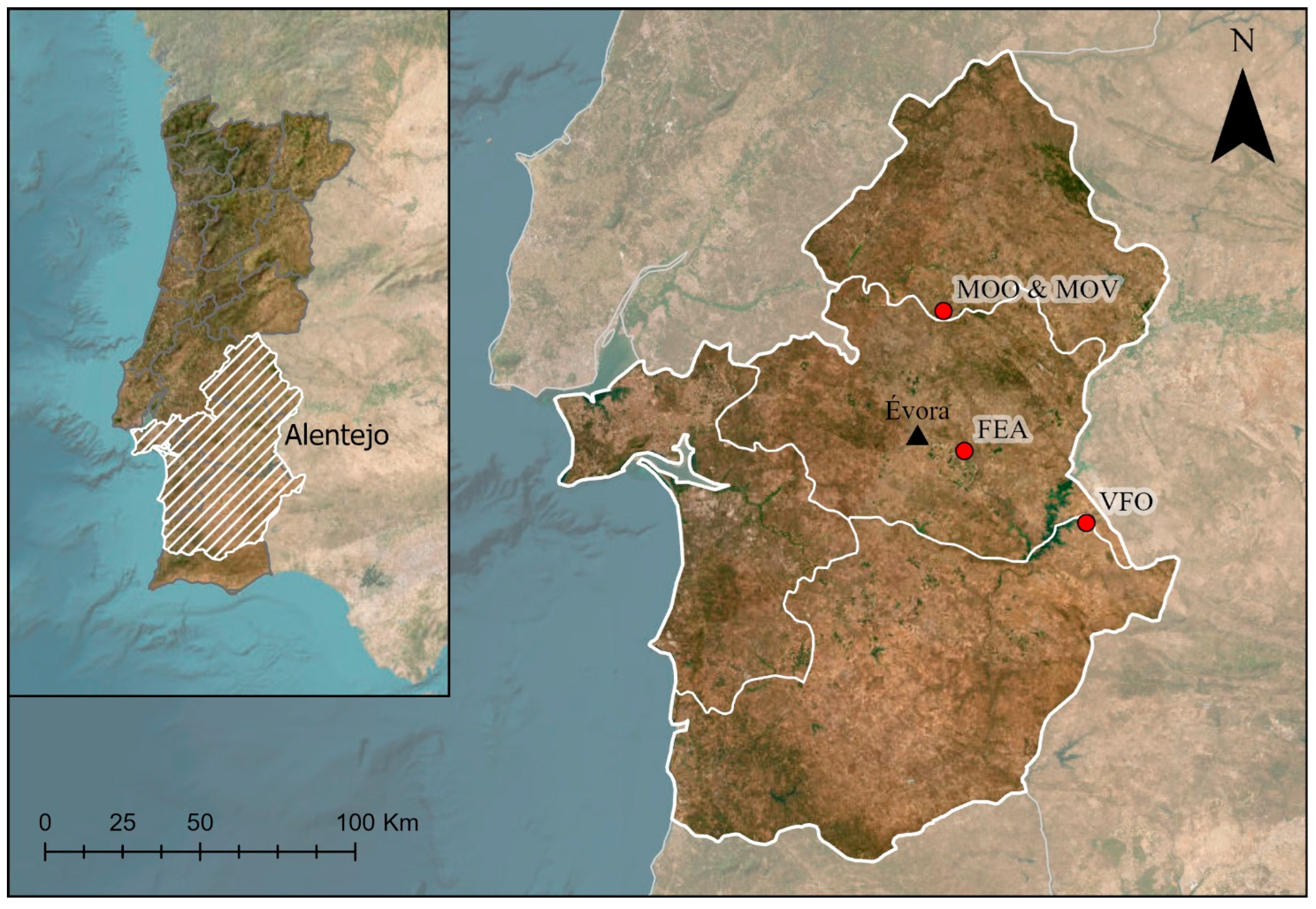
Figure 2.
Transects showing the heights of the GPS points versus the corresponding heights in the DTMs, and the RMSE values calculated from the differences between GPS and DTM heights.
Figure 2.
Transects showing the heights of the GPS points versus the corresponding heights in the DTMs, and the RMSE values calculated from the differences between GPS and DTM heights.
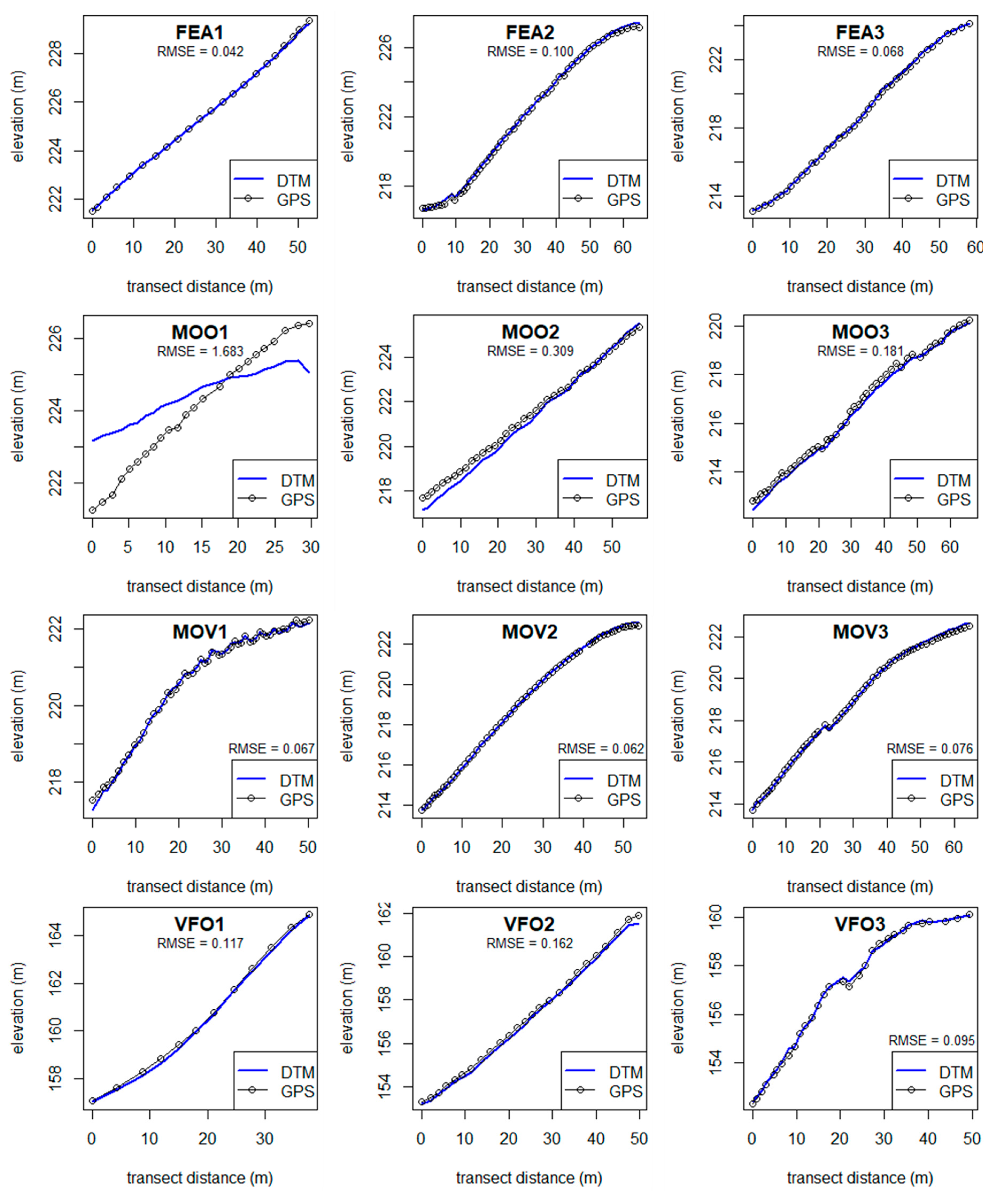
Figure 3.
Transects showing the heights of GPS points versus the corresponding height on the Co-registered and Geo-referenced DTMs.
Figure 3.
Transects showing the heights of GPS points versus the corresponding height on the Co-registered and Geo-referenced DTMs.
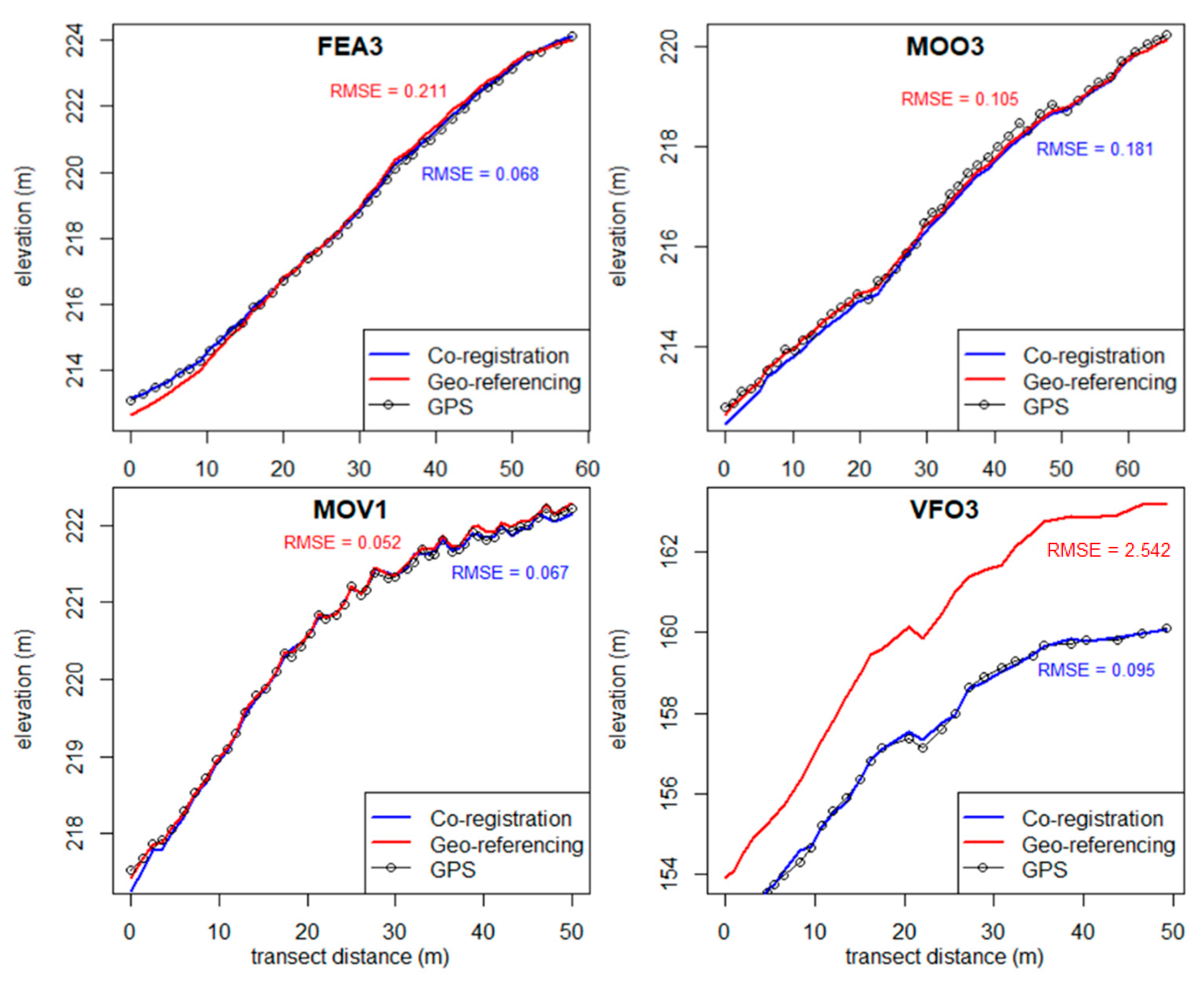
Figure 4.
(A) plot of predicted erosion against measured erosion. (B) Plot of relative differences. The dashed lines signify the 95% occurrence interval as determined by Nearing (2000) for replicate erosion plots, which were found to become wider at lower rates of measured erosion. .
Figure 4.
(A) plot of predicted erosion against measured erosion. (B) Plot of relative differences. The dashed lines signify the 95% occurrence interval as determined by Nearing (2000) for replicate erosion plots, which were found to become wider at lower rates of measured erosion. .
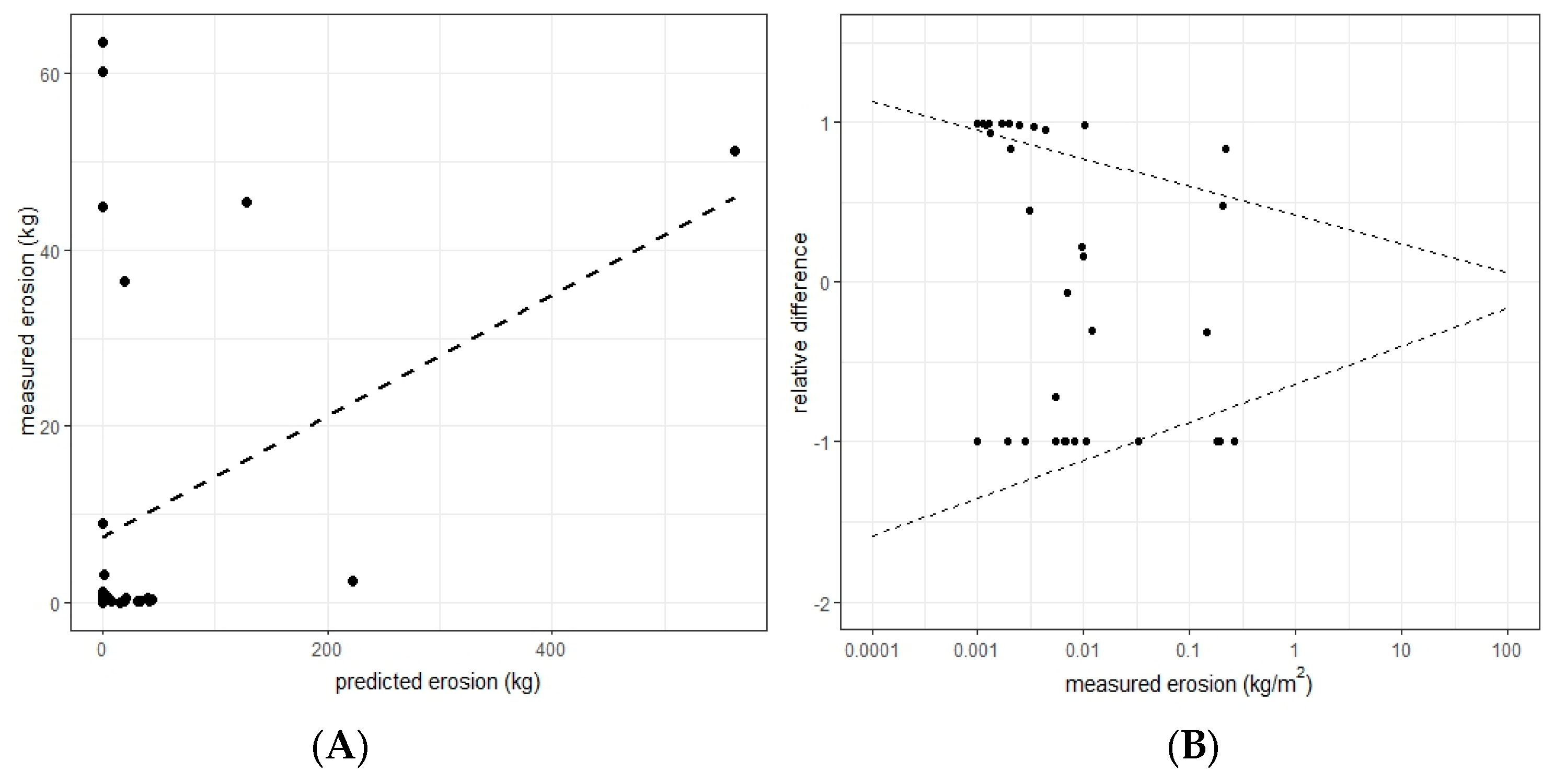
Figure 5.
Two examples of DoDs from the study areas. For each example, the first image shows the original DTM, the second image shows the DoD and the third image shows the DoD with only areas with significant increase or decrease. 5A shows a part of plot VFO8, where compaction in ruts caused by tractor passages, raising of the sides of ruts, and vegetation growth are visible. 5B shows a part of plot MOO7, where compaction in existing ruts and creation of new ruts because of tractor passages, and holes caused by soil sampling are shown.
Figure 5.
Two examples of DoDs from the study areas. For each example, the first image shows the original DTM, the second image shows the DoD and the third image shows the DoD with only areas with significant increase or decrease. 5A shows a part of plot VFO8, where compaction in ruts caused by tractor passages, raising of the sides of ruts, and vegetation growth are visible. 5B shows a part of plot MOO7, where compaction in existing ruts and creation of new ruts because of tractor passages, and holes caused by soil sampling are shown.
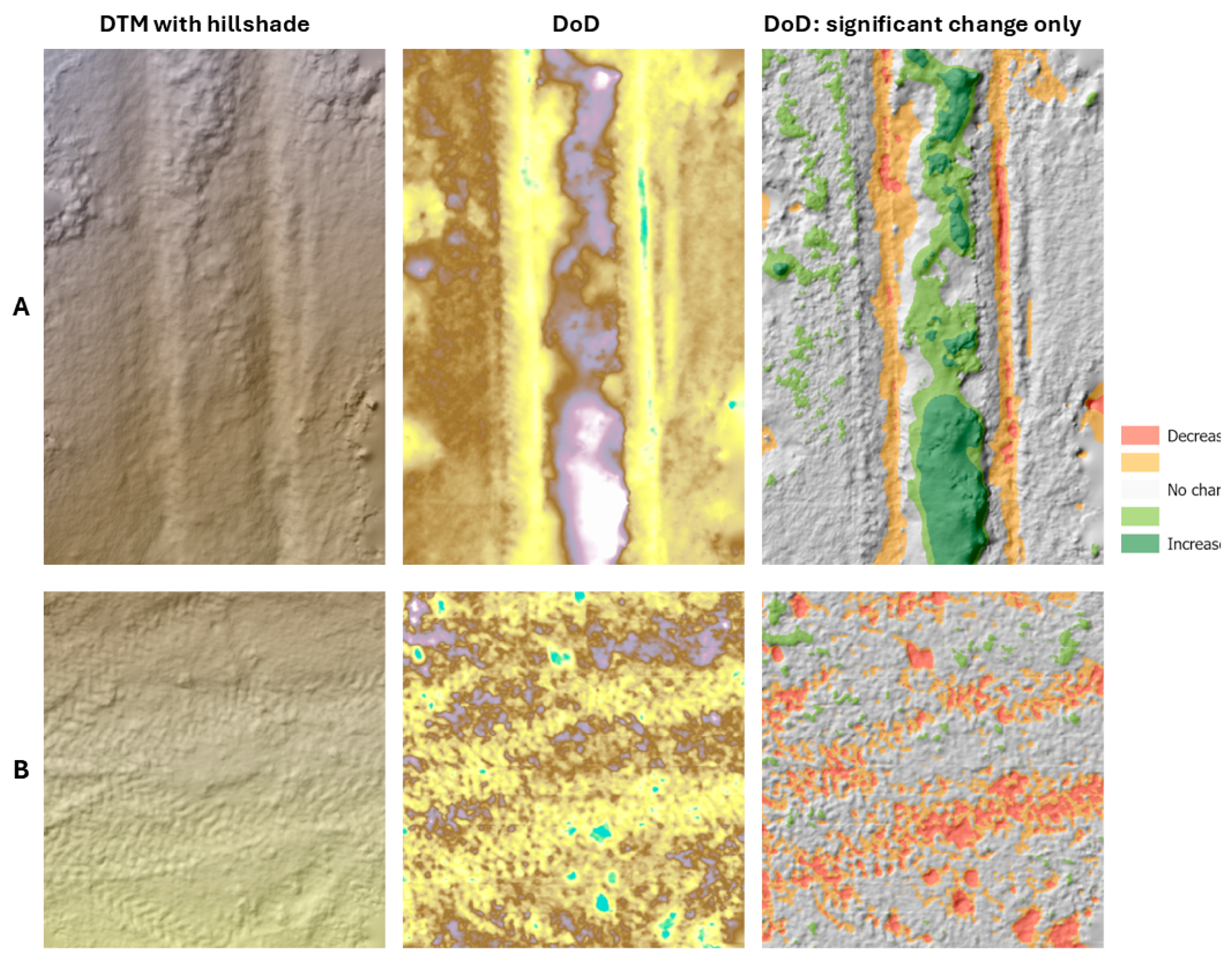
Figure 6.
Boxplots of the measured erosion, random roughness, and vegetation cover. The boxplots are separated over the study areas (FEA, MOO, MOV, VFO). The color of the boxplot shows the treatment, with red for control, green for much, and blue for mulch + biochar.
Figure 6.
Boxplots of the measured erosion, random roughness, and vegetation cover. The boxplots are separated over the study areas (FEA, MOO, MOV, VFO). The color of the boxplot shows the treatment, with red for control, green for much, and blue for mulch + biochar.
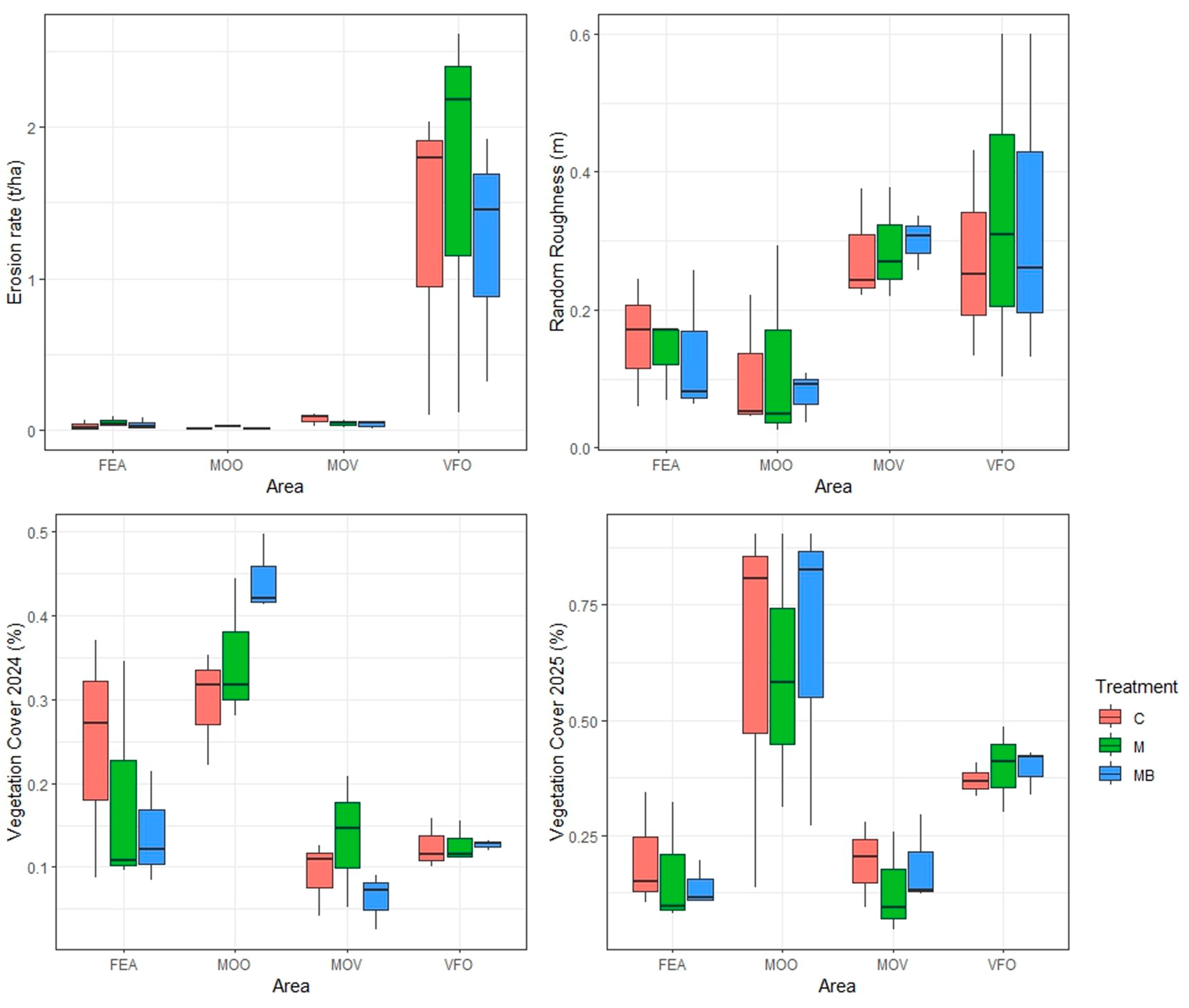
Figure 7.
(A): correlation matrix of the UAV-derived variables and in-field measured erosion. (B): Forest plot showing the results of the best performing regression model. For each predictor, the magnitude of the regression coefficient is shown by the blue circle, and the 95% confidence interval of the coefficient is shown by the blue line. On the right, the p-value of each predictor in the model is shown. The predictor “Slope x length” signifies an interaction between the two predictors.
Figure 7.
(A): correlation matrix of the UAV-derived variables and in-field measured erosion. (B): Forest plot showing the results of the best performing regression model. For each predictor, the magnitude of the regression coefficient is shown by the blue circle, and the 95% confidence interval of the coefficient is shown by the blue line. On the right, the p-value of each predictor in the model is shown. The predictor “Slope x length” signifies an interaction between the two predictors.
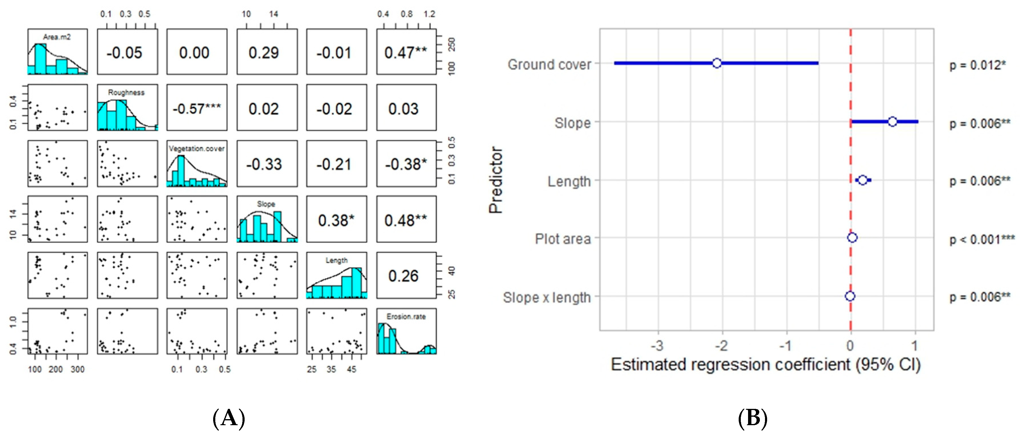

Table 1.
Table summarizing the plots per location and treatment. Each plot was given a code according to its study area (VFO, MOO, FEA, MOV). Furthermore, the plots were numbered and were assigned a code for the applied treatment (C = control, M = mulch, MB = mulch + biochar). Per study area plots were divided into three blocks (e.g., VFO1, VFO2, and VFO3).
Table 1.
Table summarizing the plots per location and treatment. Each plot was given a code according to its study area (VFO, MOO, FEA, MOV). Furthermore, the plots were numbered and were assigned a code for the applied treatment (C = control, M = mulch, MB = mulch + biochar). Per study area plots were divided into three blocks (e.g., VFO1, VFO2, and VFO3).
| Block | Olive grove | Vineyard | ||
|---|---|---|---|---|
| VFO | MOO | FEA | MOV | |
| 1 | VFO1_C VFO2_M VFO3_MB |
MOO1_MB MOO2_M MOO3_C |
FEA1_C FEA2_M FEA3_MB |
MOV1_C MOV2_M MOV3_MB |
| 2 | VFO6_C VFO7_M VFO8_MB |
MOO4_C MOO5_MB MOO6_M |
FEA4_MB FEA5_M FEA6_C |
MOV4_MB MOV5_C MOV6_M |
| 3 | VFO9_C VFO10_MB VFO12_M |
MOO7_MB MOO8_C MOO9_M |
FEA7_M FEA8_C FEA9_MB |
MOV7_M MOV8_C MOV9_MB |
Table 3.
Overview of the drone surveys, curtesy of Cambisol. The number of images was the same during both surveys and includes nadir (n) and oblique (o) images. GPS points collected in 2024 include the ground control points (gcps). GPS points collected in 2025 includes the transect points measured in the field (tran), and the co-registration points (co-reg). Low and high altitudes are given in meters above sea level (m.a.s.l.).
Table 3.
Overview of the drone surveys, curtesy of Cambisol. The number of images was the same during both surveys and includes nadir (n) and oblique (o) images. GPS points collected in 2024 include the ground control points (gcps). GPS points collected in 2025 includes the transect points measured in the field (tran), and the co-registration points (co-reg). Low and high altitudes are given in meters above sea level (m.a.s.l.).
| Study site | Number of drone images |
GPS points collected in 2024 |
GPS points collected in 2025 |
Low alt. (m.a.s.l.) |
High alt. (m.a.s.l.) |
|---|---|---|---|---|---|
|
FEA1 FEA2 FEA3 |
26(n) 52(n+o) 29(n) |
10 (gcps) 6 (gcps) 8 (gcps) |
22(tran) + 67(co-reg) 53(tran) + 48(co-reg) 41(tran) + 58(co-reg) |
219 213 211 |
229 228 225 |
|
MOO1 MOO2 MOO3 |
132(n+o) 72(n+o) 78(n+o) |
6 (gcps) 9 (gcps) 8 (gcps) |
44(tran) + 12(co-reg) 38(tran) + 18(co-reg) 46(tran) + 43(co-reg) |
214 215 210 |
226 228 222 |
|
MOV1 MOV2-3 |
20(n) 36(n) |
6 (gcps) 7 (gcps) + 8 (gcps) |
51(tran) + 51(co-reg) 117(tran) + 64(co-reg) |
216 213 |
223 223 |
|
VFO1 VFO2 VFO3 |
95(n+o) 77(n+o) 70(n+o) |
9 (gcps) 7 (gcps) 8 (gcps) |
12(tran) + 53(co-reg) 25(tran) + 49(co-reg) 50(tran) + 53(co-reg) |
154 156 151 |
171 163 161 |
Table 4.
Summary statistics of the 2025 DTMs showing the resolution of the DTM (cell size) in meters, the residual error, the RMSE between the 2025 DTM and the GPS transect, and the Level of Detection calculated for a 95% confidence interval.
Table 4.
Summary statistics of the 2025 DTMs showing the resolution of the DTM (cell size) in meters, the residual error, the RMSE between the 2025 DTM and the GPS transect, and the Level of Detection calculated for a 95% confidence interval.
| DTM | Resolution (m) | RMSE | 95% LoD (m) | |
|---|---|---|---|---|
| Vineyard | FEA1 | 0.0154 0.0180 0.0176 0.0175 0.0175 0.0171 |
0.042 0.100 0.068 0.067 0.062 0.076 |
0.117 0.278 0.188 0.187 0.172 0.211 |
| FEA2 | ||||
| FEA3 MOV1 MOV2 MOV3 | ||||
| Olive Orchard | MOO1 MOO2 MOO3 VFO1 |
0.0166 0.0190 0.0169 0.0135 0.0146 0.0164 |
1.683 0.309 0.181 0.117 0.162 0.095 |
4.665 0.858 0.502 0.325 0.450 0.264 |
| VFO2 VFO3 |
Table 5.
Table showing a summary of the ANOVA tests. The first column shows the investigated variable, The second and third column show if there were significant differences and p-values for treatment and location respectively. The fourth column shows the significant pairs and their p-value according to the pairwise comparison.
Table 5.
Table showing a summary of the ANOVA tests. The first column shows the investigated variable, The second and third column show if there were significant differences and p-values for treatment and location respectively. The fourth column shows the significant pairs and their p-value according to the pairwise comparison.
| Variable | Significant differences | Significant pairs | |
|---|---|---|---|
| Treatment | Location | ||
| Measured erosion | No (p = 0.858) | Yes (p < 0.001) | VFO – FEA (p < 0.001) VFO – MOO (p < 0.001) VFO – MOV (p < 0.001) |
| Random roughness | No (p = 0.929) | Yes (p < 0.001) | VFO-FEA (p = 0.024) MOV-MOO (p = 0.004) VFO-MOO (p = 0.001) |
| Vegetation cover 2024 | No (p = 0.814) | Yes (p < 0.001) | MOO-FEA (p = 0.002) MOO-MOV (p < 0.001) MOO-VFO (p < 0.001) |
| Vegetation cover 2025 | No (p = 0.915) | Yes (p = 0.002) | MOO-FEA (p = 0.002) VFO-FEA (p = 0.020) MOO-MOV (p < 0.001) MOO-VFO (p < 0.001) |
Disclaimer/Publisher’s Note: The statements, opinions and data contained in all publications are solely those of the individual author(s) and contributor(s) and not of MDPI and/or the editor(s). MDPI and/or the editor(s) disclaim responsibility for any injury to people or property resulting from any ideas, methods, instructions or products referred to in the content. |
© 2026 by the authors. Licensee MDPI, Basel, Switzerland. This article is an open access article distributed under the terms and conditions of the Creative Commons Attribution (CC BY) license (http://creativecommons.org/licenses/by/4.0/).
Copyright: This open access article is published under a Creative Commons CC BY 4.0 license, which permit the free download, distribution, and reuse, provided that the author and preprint are cited in any reuse.