

Submitted:
22 March 2026
Posted:
24 March 2026
You are already at the latest version
Abstract
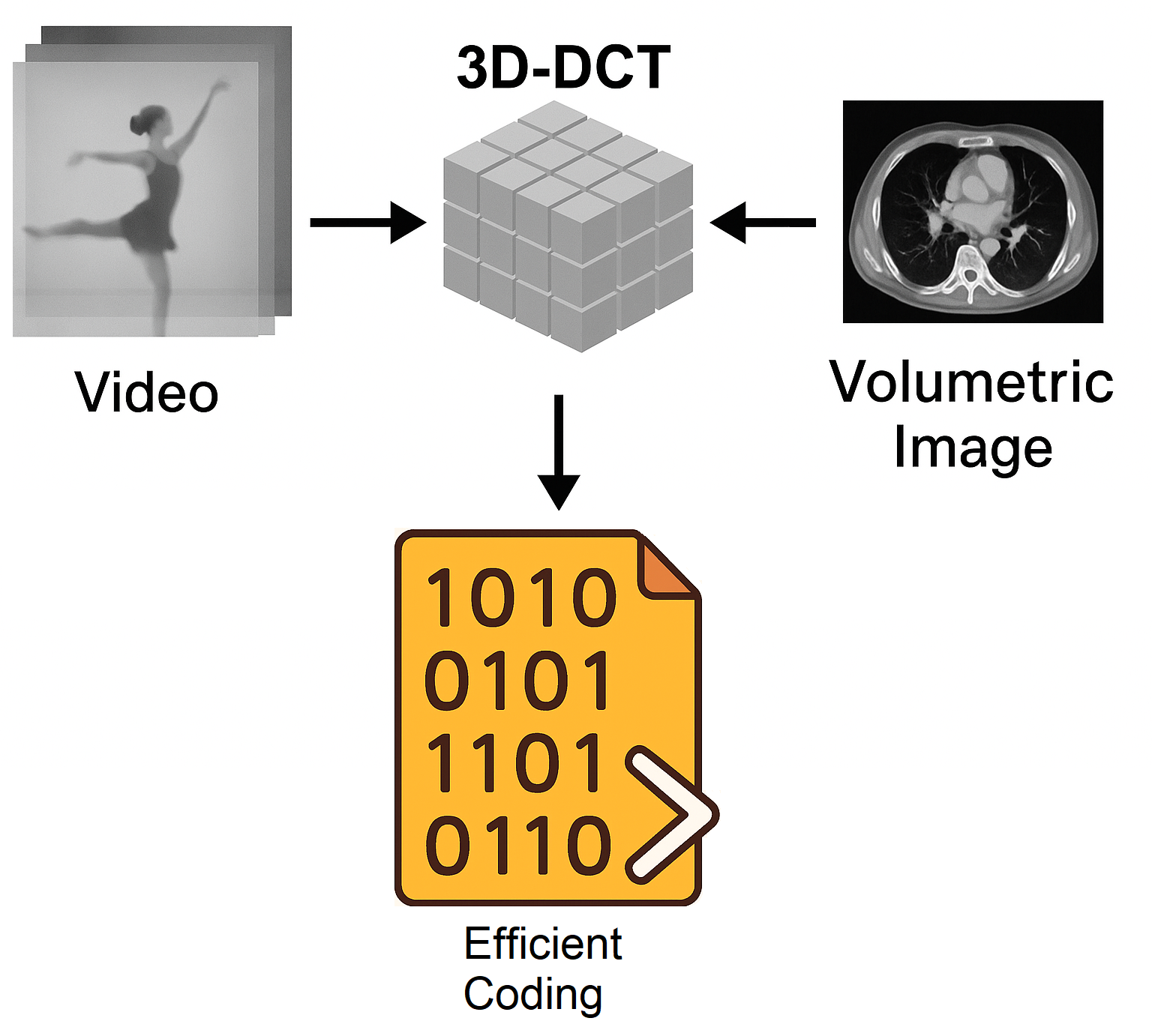
This paper evaluates the practical use of the Three-Dimensional Discrete Cosine Transform (3D-DCT) for video and volumetric image compression. While one- and two-dimensional DCT transforms are widely used in modern multimedia standards, their three-dimensional extension has received limited attention in real coding systems. In this work, a complete 3D-DCT–based encoder is developed by extending a JPEG-like pipeline to operate on three-dimensional data blocks. The proposed approach processes groups of video frames as 3D cubes and applies a separable 3D-DCT followed by quantization, coefficient serialization, and entropy coding. Unlike conventional video codecs that rely on motion estimation and compensation, the proposed system exploits temporal redundancy directly through the transform domain, resulting in a simpler coding structure with reduced algorithmic complexity. Different configurations are evaluated, including alternative methods for computing the 3D quantization matrix, serialization schemes, and variable block depth along the temporal dimension.Experimental results obtained from multiple test videos and volumetric medical datasets, including CT and MRI studies, demonstrate that the proposed method achieves competitive compression ratios while maintaining good reconstruction quality measured in terms of Peak Signal-to-Noise Ratio (PSNR). The results indicate that 3D-DCT provides a flexible and computationally simple solution for both video compression and three-dimensional medical image coding, particularly in applications where implementation simplicity and frame-level accessibility are important.
Keywords:
image transforms
; discrete cosine transform
; video coding
; medical images coding
1. Introduction
Nowadays, the distribution and archiving of video is a daily routine. Digital broadcasting platforms, traditional broadcasting systems (now converted into digital ones), social networks, private applications like surveillance security systems, and many other examples produce worldwide thousands of videos each day. Optimized coding of video means converting the raw output from camera sensor to a reduced format that can be efficiently distributed or archived. Note that size of a regular High Definition (HD) video of 1920×1080 pixels, Red-Green-Blue (RGB) color space (three color channels) and 25 frames per second would be: 1920×1080×3×25= 155×106 bytes/s assuming 8 bytes per sample (the usual value), this is 1.2 Gbit/s. This huge bitrate would make impossible the actual use of video technology. That same video is reduced to only 5 Mb/s using modern MPEG-4 coding (the technology used nowadays in digital television systems). This example illustrates the importance of video coding technology. Multimedia applications would not exist without it [1].
Mathematical image transforms have always played a central role in the still image and video coding methods. This is because of their ability to concentrate spatial image information in a small set of numerical coefficients. Discrete Cosine Transform (DCT) [2] and its variants have become the most used concept for this task. The 2D-DCT serves as the foundation for the JPEG standard in still image compression and plays a crucial role in widely used video coding standards such as MPEG-1, MPEG-2, H.261, and H.263. More advanced codecs, including MPEG-4/H.264 and the latest MPEG-H/H.265, utilize an enhanced version of the 2D-DCT. Furthermore, a variation of the 1D-DCT, known as the Modified Discrete Cosine Transform (MDCT), is commonly used in audio coding.
This work explores a less known variant known as 3D-DCT that is the natural extension to a 3D image (a voxel made image) than can also be constructed stacking the individual frames of a video.
Let x be a monochrome square image. This image is mathematically represented as a discrete matrix or function of two integer variables: x[m,n] (m,n=0...N-1). Under these conditions, the two-dimensional discrete cosine transform (2D-DCT) of x is defined as (Sx) [3]:
where:
This definition, as can be deduced from the equation, allows obtaining a new real matrix (no imaginary part) of the same size (N×N). It can be shown that, when applied to low-pass spectrum images (all natural images and those synthetic images that look natural), most of the information is concentrated in the first coefficients: the Sx[u,v] with u+v of small value. This fact is simply due to the concentration of information at low frequencies. The u and v indices can be understood as horizontal and vertical spatial frequencies [4].
The qualitative properties of the DCT are very similar to those of the Fourier transform. An FFT-2D would also concentrate the information at low frequency but, in this case, we would have a non-zero imaginary part and a replication of the transform values at multiples of N (periodicity in the two spatial frequencies with period 2π). See graphical representation of an example in Figure 1.
Of course, for DCT, there is a reversal equation that allows the original image to be recovered exactly:
Widely used methods, such as JPEG, MPEG-1 and 2 standards, H.261 and H.263 are based on dividing the images into small square blocks (the size used in these standards is 8x8), calculating the 2D-DCT transform of each block and quantifying the S coefficients Sx[u,v].
This work consists in studying the extension to three dimensions of the DCT concept, i.e., starting from a three-dimensional (cubic) matrix of real values: x[m,n,p] (m,n,p=0...N-1), the 3D-DCT is defined as (analysis equation):
In addition, the inversion equation (or synthesis equation) would yield:
This concept has already been formulated, although it is not very well known. It has been used for video coding [5] and also for coding videos obtained in medical explorations (endoscopy) [6]. In addition, there exist fast algorithms for 3D-DCT computation [7].
In this paper, the 3D-DCT is implemented in MATLAB (The MathWorks, Inc., Natick, MA) for video coding, developing a novel coder that is analyzed in various scenarios. Notably, its application to medical 3D studies presents a promising new avenue for exploration. This new coding scheme is not intended to replace lossless standards such as JPEG 2000 [8] or JPEG-LS [9]. However, it provides an effective alternative for storing large volumes of legacy data or supporting rapid communication scenarios, as it achieves significantly higher compression rates.
With respect to precedents [5] and [6], authors in [5] focus on optimizations for low power applications: Internet of Things (IoT) and drones, while our study focuses on constructing a solid method from scratch and exploring all possible applications. Furthermore, the method presented in [6] is very specific to endoscopic video characteristics whereas this study is much more general. The proposed method is amenable to implementation on dedicated hardware and is therefore well suited for low-power environments. Importantly, motion detection and motion compensation constitute the primary computational burden in MPEG and H.26x codecs; by contrast, the system introduced in this paper does not rely on these processes.
As another contribution of this paper, a non-cubic (parallelepipedic) version of ·3D-DCT with a deeper excursion of the p index in equations 3 and 4 has been implemented and tested in all previously described scenarios obtaining novel and interesting results.
Other interesting specific studies about 3D-DCT are, for example: [10] where authors demonstrate that 3D-DCT coding can be more robust against transmission errors. In [11] a study is presented on quantization and ordering of 3D-DCT coefficients proposing adaptive schemes. Authors of [12] study the transform coefficients to predict which of them will be zero and optimize the computation. In [13] a system for digital mobile devices is described, authors base themselves on the methods described in [12].
In [14] authors do an extensive review of medical image compression. According to them, most examples are lossless methods that are not comparable to this development. One of the few lossy examples is [15], where authors propose detecting most interest regions using convolutional neural networks, then rest of the image is simplified using a low-pass (blurring) filter and a lossless method is used. Compression ratio for this method (2.25) is much less than the values achieved by a DCT based lossy system whereas diagnostic quality can be demonstrated with the same objective measurements: Peak Signal to Noise Ratio (PSNR) and Structural Similarity Index Measure (SSIM).
Main contributions of this paper can be summarized as follows: This paper investigates the practical use of the Three-Dimensional Discrete Cosine Transform (3D-DCT) for video and volumetric image compression. The main contributions are as follows:
- A complete 3D-DCT–based coding framework: A simple and fully functional end-to-end codec is developed by extending a JPEG-like 2D pipeline to three dimensions, including 3D transform computation, quantization, serialization, and entropy coding.
- Low-complexity video compression without motion compensation: The proposed approach exploits temporal redundancy via 3D-DCT, achieving compression performance comparable to MPEG-4 while avoiding motion estimation and compensation, significantly reducing computational complexity.
- Editing-friendly video coding with configurable GOP sizes: The use of fixed-size 3D blocks enables short and flexible GOPs, allowing direct frame access and making the method well suited for video editing workflows and camera firmware.
- Generalization to non-cubic 3D-DCT blocks: Non-cubic (parallelepipedic) 3D-DCT transforms are introduced and evaluated, demonstrating that increasing the third-dimension size improves compression efficiency across applications.
- Novel 3D quantization and serialization strategies: Two original methods for 3D quantization matrix construction and two alternative coefficient ordering schemes are proposed and analyzed, showing that optimal choices depend on the redundancy structure of the data.
- Application to volumetric medical image compression: The proposed coder is successfully applied to real CT datasets, achieving very high compression ratios while maintaining diagnostically acceptable image quality.
2. Materials and Methods
2.1. Starting Point
This work was initially conceived as an exploration of how to create a video coder from a standard JPEG coder designed for still images. Initially, a functional code designed by authors is used. This code implements still image JPEG encoding and it is very simple (pseudo-code in Figure 2).
In the code, we can see how the image is divided into small square blocks of the same size as the quantization matrix: Q. Normally, Q is of size 8x8 but the present code can work with any square size.
The cosine transform in two dimensions is applied to each of the original blocks (line 13). The values of the cosine transform are quantized. The matrix Q contains a different quantization step: Qij for each DCT coefficient, according to its position or importance). The next step is the zig-zag sorting of the coefficients in order of importance (line 14). Note that, to generate a sequence of data that can be saved in a file, it will always be necessary to serialize the matrices (reorder them as vectors). The zig-zag serialization (Figure 3) places the least significant coefficients at the end. This, for natural images, produces long series of zeros at the end of the quantized and serialized block (because the high-frequency coefficients are weak and are quantized more strongly). These series of zeros (in a typical JPEG encoding there are more than 90% of zeros at this stage) allow a high compression of the data, using an end-of-block binary code in the final binary sequence. In line 16, a variable length binary encoding (Huffman code) is applied, which will be responsible for the reduction in the size of the information. In addition to introducing the end-of-block code at the time when the remaining coefficients are a series of zeros, the significant part is also encoded using shorter codes for more probable values and vice versa.
The standard does not specify compulsory values for the coefficients of the Q matrix [16,17,18,19,20]. There exist various classical papers about coefficient optimized quantization. Nevertheless, most implementations use the values recommended in [21] that are the JPEG official recommendation, see equation 5 for the numerical values.
This matrix is used to achieve an average quality (q=50%). To achieve higher qualities (50<q<100) it is multiplied by a factor: 2-q/50, always less than 1, achieving smaller quantification steps. For q<50 the factor is 50/q, greater than 1, which increases the quantification steps.
The exercise consists, of converting this still image coder into a video encoder using the concept of 3D DCT and stacking consecutive frames of the video in order to obtain cubic three-dimensional blocks of size 8x8x8. Applying a non-cubic 3D-DCT means using non-cubic blocks of size 8x8xZ where Z can be any integer number, generally greater than 8. In the vocabulary of video coding this new coder would use fixed size GOP’s (Groups of Pictures) of Z frames. In video coding, a Group of Pictures (GOP) is a sequence of frames that are encoded with interdependencies to enhance compression efficiency via temporal redundancy.
Before the video (3D) extension, this JPEG encoder is assessed with a collection of uncompressed grayscale images (bmp format) including some of the most historically used (Lenna, Cameraman). A total of fourteen images. The results obtained for the Q matrix of (5), q=50, are PSNR 34 dB and compression ratio 9.40 or 9.40:1 (original-size/compressed-size).
In everything that follows, PSNR (Peak Signal to Noise Ratio) is defined as:
where Nbits is the number of bits per sample in the initial format, is the initial image/video and is the image/video obtained after the coding and decoding process. PSNR is a common manner of measuring the quality of a coding method [3].
Compression rates will be measured as a ratio obtained dividing the original bit size of the image/video and the bit size of the coded format. Many times this ratio is converted to bpp’s (bits per pixel), bpp’s = Nbits/Compression-ratio. For example, for the previous example of JPEG compression of still images, the average compression ratio of 9.40 yields 0.85 bpp.
In the following subsections a description is provided for the basic building blocks that were created to make possible the easy extension to a 3D (video) coder.
2.2. 3D-DCT Computation by Separability
To implement the calculation of the three-dimensional DCT, we need to develop a new function, since there is no such extension in the MATLAB catalog.
For this purpose, an advantage is taken of the separability property. That is, a 2D transform is separable if it can be written in this way:
Where X is the input image (matrix), S is the transform (matrix) and C is the matrix that defines the transformation. The first product in equation 7, would be the 1-D transform of the columns of X, while the second would be the 1-D transform of the rows. That is: the 2-D transform can be calculated through 1-D transforms: it can be done first by rows and then by columns or vice versa, and the result is the same.
The DCT is separable, in terms of 6, we would have to do:
with i and j in a range between 1 and N.
Applying this to a three-dimensional case, given an input parallelepiped x[m,n,p], the DCT-3D can be calculated:
- First, apply the DCT-2D to each 2D layer of x: x[m,n,p0 ] (p0 constant).
- Applying in the resulting matrix, the DCT-1D (dct function in MATLAB), to each vector T2d[m0 ,n0 ,p] (m0 and n0 constant).
2.3. From the Quantization Matrix to the Quantization Parallelepiped
Now it is necessary to calculate a three-dimensional quantization matrix. That is a quantization cube or parallelepiped, mathematically a tensor. Calling this object Q3, it will be a matrix with three indices Q3(i,j,k) where the indices i,j indicate spatial frequencies whereas k will be a temporal frequency. Intuitively, the values of Q3 should grow as the sum i+j+k increases.
Two methods for computation of quantization coefficients were implemented and tested:
-
Method 1: called the geometrical method. To easily calculate an operational matrix, the following method has been designed:
- Make the matrices corresponding to the Cartesian planes, that is Q3(i,j,1), Q3(i,1,k), and Q3(1,j,k) equal to the original JPEG matrix (equation 5). If Z dimension (index k) is greater than 8, remaining values are filled with the maximum value in the 2D matrix.
- Calculate the remaining values according to the plane i+j+k=c0 to which they belong.
- For a plane, i+j+k=c0, make its coefficients Q(i,j,k) not yet assigned; equal to the average of those already assigned (the values already assigned are those on the intersection lines of that plane with the Cartesian planes).
- If there is no intersection. For these high frequencies, make Q3(i,j,k) equal to the maximum coeffient of 2D matrix.
The idea behind this method is making a geometric extension of the original JPEG matrix.
-
Method 2: called the polynomic method. This new method comes from the idea of constructing polynomial function that computes matrix coefficients. Method details are:
- Assume that there exists a function that can compute Q2(i,j) as:
- 2.
- Compute A, B, and C, using a overdetermined linear equation system solved using a matrix formulated minimum square error method [22].
- 3.
- Extend the polynomial for being able to create a 3D Q, Q3(i,j,k):
- 4.
- Coefficients must be corrected using the following empirical equations:
- 5.
- Running a simple loop allows to create a 3D Q matrix easily (computed coefficients are rounded to the nearest integer). Remember that any matrix is valid, its ability to get high PSNR and high compression must be tested.
Note that the DCT-3D will have a different scaling. According to equation 1, the maximum value of a DCT-2D is max_lumxN (continuum coefficient of a constant block equal to the maximum luminance value). For the typical situation: max_lum=255 and N=8, a maximum value of 2040 is obtained. In DCT-3D (equation 3), the maximum will be max_lumxNx(Z)0.5. For the same case, a maximum of 5770 is obtained for N=Z=8 (cubic transform). This data seems to suggest that the Q3 matrix could be scaled by a factor of 5770/2040 = 2.83, maintaining the quality/compression ratio. This is an estimate; obviously, it must be tested with real videos since the temporal redundancy in the third dimension is not going to be equal to the spatial redundancy. Experiments have been performed with the Q3 matrix derived from the original Q, without scaling, obtaining satisfactory results: see section 3.
2.4. Serialization of the Quantized Block
Serialization is simply a way of ordering the coefficients of the transformed matrix already quantized. It should be an ordering by perceptual importance, or in other words: an ordering that favors the appearance of long series of zeros, especially at the end of the block, so that variable-length coding (lossless compression) is very efficient.
To perform the 3D transform path, it was experimentally verified that, in regular videos, 90% of the non-zero coefficients of the block are in the first layer: T3d[i,j,1], where the third dimension is the temporal one. This can be due to the higher temporal redundancy, compared to the spatial one.
Two methods for serialization were implemented and tested:
- Method 1: Based on the fact stated above, the serialization is performed by horizontal plane layers: T3d[i,j,k0], with constant k0. The word horizontal means that layers are parallel planes orthogonal to vector (0,0,1). Inside each layer, the zig-zag path inherited from the standard JPEG method is applied.
- Method 2: In theory, indexes i, j, and k are proportional to transform frequencies (horizontal, vertical and temporal), so the sum i+j+k can be used as a measurement of “how high is the frequency associated with a given coefficient”. So it can be reasonable to order coefficients using parallel planes orthogonal to vector (1,1,1), id EST: planes with equation the i+j+k=c0.
The second method will be better when redundancy is similar when moving on any of the three axes. More concretely, “horizontal” planes are optimum in video coding because of redundancy being greater in the temporal dimension; if applied to 3D volumetric data, second method is best.
From now on, system running with method 1 on each option, will be called the baseline coder. In the results sections performance is compared for baseline coder and all the variations.
2.5. Variable Length Encoding
This section does not change compared to the 2D view. However, we will comment a little on its implementation.
For this purpose, the tables published in [23] are used. The implementation employs DC and AC coefficient encoding from the JPEG Baseline Encoder (ISO/IEC 10918-1). Huffman coding represents both the length of any intermediate run of zeros and the size of the coefficient codeword. Each coefficient is then encoded in one’s complement, with the most significant bit indicating its sign. The sequence “1010,” or End of Block (EOB), signals that the remaining coefficients are zero, allowing the encoder to proceed to the next block.
2.6. Video Encoding with 3D-DCT
With all these ingredients, monochrome video coding can be implemented with a simple code very similar to the original one in Figure 1. In Figure 4, we can see how the video is represented with a three-index matrix that is divided into cubes to which the same process is applied: transform, quantization, serialization, and Huffman coding.
2.7. Test Videos
Twenty-three test videos will be used. All of them are color videos in .y4m format (without compression). Among them are some very popular in MPEG testing like Akiyo, Foreman, Claire, or Miss America. A function obtained from MATLAB Central [24] is used to read this format. This function returns a movie object from which the Y, Cb, Cr components required for encoding can be easily extracted (for monochrome video the Y component is enough). Videos were obtained from [25], see Appendix A for a description of video collection.
Note that, unlike machine learning systems, a coding scheme does not need a massive dataset for testing.
3. Results and Discussion
3.1. Monochrome Video Encoding
Results for all coder variations are summarized below in Table 1, average bitrates are not computed because collection consists of videos of different resolutions and it is difficult to compare.
The comparison with popular MPEG-4 is done using videowriter MATLAB function with default options: 90 frames GOP with one I frame, 44 P frames and 45 B frames). This results in a PSNR of 43 dB (better than all 3D-DCT methods) and a compression ratio of 27 that is less than those achieved by almost all 3D-DCT options.
Nevertheless, 3D-DCT offers practical advantages for specific use cases. Because it does not require motion detection or compensation, it is simpler than many alternative methods and is therefore well suited for encoders operating on resource-constrained devices.
Another important benefit is that 3D-DCT enables the selection and editing of individual frames without the need to decode large GOPs of 30, 60, or 90 frames (GOP: Group of Pictures, a sequence of frames linked through motion prediction). With 3D-DCT, a GOP typically contains only 8, 16, or 32 frames. This flexibility is particularly valuable for video production companies, which currently rely on formats without temporal redundancy—such as DV-25 and DVC-Pro—that use a GOP of a single frame. However, these formats are significantly less efficient than 3D-DCT, making the latter a more effective alternative for such workflows.
The last three rows in Table 1 report the results of a test run using the H.265 (HEVC) codec. This experiment was conducted by combining a MATLAB script with FFmpeg [26] as an external encoder. H.265 currently achieves higher compression rates than both MPEG-4 and 3D-DCT. Nevertheless, the considerations discussed above regarding specialized applications remain valid.
From Table 1, it can be inferred that the second method for computing Q values yields a more efficient system, paying slightly worse PSNR but much better compression. Regarding DCT ordering, PSNR value is the same except for rounding errors, regardless of the serialization method used because of the fact that quantized coefficients are the same. Compression is better for the method 1 confirming the assumption of bigger temporal redundancy. Effect on variation in Z is, in general, a better performance for greater Z values (increasing both PSNR and compression ratio). In particular, variation 10 is able to outperform outstandingly MPEG4 baseline improving compression more than 100% (notice that H.265 outperforms MPEG4 only with 30-50% improvement). Note also that PSNR’s over 30 are enough, making not so important the advantage in PSNR shown by MPEG.
To enable an appropriate performance evaluation, the graph in Figure 5 was generated. The performance factor (PF) is defined as the product of PSNR and the compression factor. Using the MP4 baseline as a reference (PF₀), the normalized performance factor is computed as PFₙ = PF / PF₀. Values greater than 1.0 indicate better performance than the MP4 baseline, whereas values below 1.0 indicate inferior performance.
The last column reports the processing time (in seconds), calculated as the average of encoding and decoding time per frame for each configuration. The MATLAB implementation used for prototyping is noticeably slow (tests were conducted on an AMD Ryzen 7 5700G at 3.80 GHz). Real-time performance can be achieved through optimized low-level programming in languages such as C or C++. Accordingly, MATLAB should be regarded as a prototyping environment rather than a platform for final deployment.
In this implementation, a substantial portion of the execution time is attributable to Huffman coding, which is typically faster in lower-level languages. Operations requiring bitwise manipulation and associative table searches are not well optimized in MATLAB. By contrast, all MPEG variants rely on motion detection and compensation, processes that are inherently computationally expensive.
Execution time also decreases as the GOP size increases. This suggests that, although the DCT constitutes the primary computational burden, its cost does not scale linearly with transform depth; in fact, the transform time appears nearly constant. It should be noted that the reported averages were computed only for CIF (352×288) videos; Appendix A provides a detailed description of the video dataset.
A brief study about computational load is included in Appendix B.
3.2. Color Video Encoding
The color video is encoded in the same way as monochrome video: by running the encoding three times, once for each component (Y, Cb, and Cr). The chroma components are under-sampled with a 4:2:0 scheme (dividing both the width and height of each frame by 2), as in MPEG. In addition, a different matrix is used for color coding (Q3c), obtained from the Qc matrix of the 2D-JPEG (which has slightly larger quantization steps, see equation 7).
The average results for baseline coder are now: 33.33 dB PSNR, and an average compression ratio of 77.91. For MPEG-4 we obtain 36.10 dB PSNR (8% better) and 65.20 compression ratio (14% worse). Again a draw, or not if bitrate is considered the main parameter (assuming that PSNR > 30 dB ensures visual quality).
Results for all options are summarized in Table 2:
The conclusions remains the same. Second method for Q coefficients computation is again very efficient boosting compression ratio, in this case without even getting worse PSNR. Again, PSNR does not change with serialization method. Compression is a bit worse for the second serialization scheme. The big extra compression in the color components (Cb and Cr are decimated and subjected to more aggressive quantization) makes compression rates go higher for all coders compared to the monochrome example. Interestingly, in this test H.265 achieves superior visual quality but is less efficient in terms of compression, being surpassed by 3D-DCT. Compression was performed using FFmpeg with a fixed GOP size and a maximum of three consecutive B-frames, while coefficient quantization was handled by the encoder’s internal optimization mechanisms. The effect of the Z parameter is the same of previous section: getting better performance with increasing Z. 3D-DCT can serve as a viable alternative to MPEG in specialized environments. PF curves have been re-computed for this case, see Figure 6.
Conclusions about processing time are, basically, the same. As a comparative example, results for color compression using 3D-DCT reported in [6] are PSNR=39 dB and 18 compress ratio, this would yield a PF in Figure 6 of 0.29, clearly below the implementation described in this paper. For results published in [10], FP would yield 0.46.
3.3. Medical Images Coding
In [3], the authors use 3D-DCT for the encoding of color video from endoscopies. This should not be very different from the two previous sections.
Here a different application is tested: the encoding of 3D medical studies. A 3D medical study (best examples are Computed Tomography (CT), or Magnetic Resonance Imaging (MRI) consists of a set of monochrome images corresponding to parallel slices of areas of the human body.
These studies are usually stored in collections of files stored in a specific format for the work and exchange of medical images: the DICOM format.
However, when they are read by an application, an in-memory structure consisting of a numerical array with three indices is usually created (a 3D image made of voxels instead of pixels). This is a very voluminous piece of information that can be efficiently encoded using 3D-DCT.
Of course, any 3D-DCT-based format is not going to replace DICOM which will continue to be used on a day-to-day basis. However, some kind of compression may be interesting to facilitate faster file exchange and/or for massive archiving of old medical records.
Testing with a real CT of 460 slices (consisting on a study comprising the entire head and upper half of thoracic region), each of size 512x512 (12-bit monochrome images), the baseline coder (Z=8) yielded: 47.43 dB PSNR and a compression ratio of 116.51. The quality seems sufficient but could be increased by using a Q3 matrix scaled by a number less than 1. The original DICOM files can use different types of compression, most used are lossless schemes like JPEG-2000 lossless (JPEG-LS). Note that this is a “per slice” compression, not a method working with the whole volumetric image. If the degree of compression is measured by dividing the total size of these DICOM files by the compressed 3D-DCT size, the factor obtained is 22 (relative compression, opposed to absolute compression obtained dividing the total bit size of the volumetric image by the compressed bit size.
Extending the test to a collection of 12 CT studies that are real medical images from different body regions: full head and shoulders, dental CT and cervical spine (all of them downloaded from public sources [27,28]), results obtained for the baseline coder are: 37.56 dB for average PSNR, 318.93 average compression rate measured absolutely (relative to initial bit size) and 290.85 compression rate measured relatively to DICOM files size. Note that compression rate depends highly on the initial entropy of input data and a CT study of a head consists of much less regular images than other of the abdominal region. Besides, the relative compression rate is very dependent on the compression used in DICOM files (most DICOM files use JPEG-LS).
In Table 3, below, results are showed for all coder variations.
Comments are similar to those in previous sections. The second method for Q coefficient compression increases efficiency, losing less than 1 dB in PSNR in exchange for much more compression. Regarding serialization, quality does not change but, in this case, the behavior in compression rate is different because of the different redundancy over each axis. In this case, the second serialization improves greatly the compression performance. The reason is that redundancy is more equally distributed across axes this time. Again the effect from Z value is improving performance with increasing Z. Note the outstanding results for variation 11. MPEG is not used in this scenario and thus it is not tested.
In [9], authors recommend another merit factor for medical image compression. This parameter is called SSIM (structural similarity index measure) and it is a real number between 0.0 and 1.0. Similarly to a correlation coefficient, a value of 1.0 is maximum similarity. Computing SSIM for the test studies average results are above 0.75 for all the variants assuring a good performance for the proposed applications.
To demonstrate the capability of 3D-DCT for compressing MRI data, an identical test was conducted on three studies (see Appendix A). The original images were obtained from [28]. The results are presented in a corresponding table (Table 4). Note that the image sizes vary across the studies, which reduces the comparability of the processing time measurements.
4. Conclusions
This paper investigates the capabilities of the Three-Dimensional Discrete Cosine Transform (3D-DCT), both as a pedagogical tool and as a practical approach to video coding and medical image compression. While this was initially considered as a didactic exercise, the study evaluates its feasibility as an efficient coding technique in various applications.
The 3D-DCT presents a compelling alternative for video coding, particularly in scenarios where software simplicity is crucial, such as implementation on low-power hardware. Additionally, it outperforms formats like DV-25 and DVCpro for compressing video intended for editing, making it a strong candidate for integration into video camera firmware.
A particularly novel application explored in this study is the use of 3D-DCT in medical imaging. The results demonstrate that it provides a high quality, high-performance compression scheme, which could be valuable for three-dimensional medical studies, such as CT or MRI scan data storage and transmission.
Obtained results support the above conclusions as PSNR/Compression data for 3D-DCT method match and sometimes outperform those of MPEG-4 for monochrome and color videos (at least for the MATLAB baseline coder). It even outperforms H.265 (HEVC) for compression in color videos. Results for medical 3D studies show that use of 3D-DCT coding would be a good method for optimized archiving or rapid communication of studies.
Two methods have been used for quantization 3D matrix computation. The second one is a polynomic regression scheme and, despite of being fully heuristic, results are very interesting: getting slightly worse results in PSNR but boosting compression rate values.
Two methods have been used for DCT serialization obtaining better results for the first one in videos (high temporal redundancy) and for the second one in medical images (where all dimensions are spatial and redundancy is fairly equal in all axes). In general terms, if it is known than a given 3D direction in image cubes shows less entropy than others, serialization planes should be orthogonal to that direction.
Third dimension (Z axis) for the DCT was made variable defining a coding system with variable GOP size. Influence of the Z size value on results was an improvement on efficiency in all applications considered. Note that increasing GOP makes more difficult the use in an environment where video edition is necessary.
Although the MATLAB implementation used for prototyping is significantly slow: for example, in the case of CT compression, processing time per slice (individual 2D image) is 2.42 s for a 8 images GOP, 1.26 s for Z=16 and 0.72 for Z=32, machine was an AMD Ryzen 7 5700G at 3.80 GHz. Real-time performance can be achieved using optimized low-level programming techniques in an appropriate language like C/C++. MATLAB should therefore be viewed as a prototyping environment rather than a final implementation tool.
Future research will further investigate potential applications, particularly in 3D medical image coding, where 3D-DCT could offer a balance between compression efficiency and computational complexity. Additional optimizations and hardware-accelerated implementations could enhance its viability for real-world use.
Author Contributions
For research articles with several authors, a short paragraph specifying their individual contributions must be provided. The following statements should be used “Conceptualization, F. Martín-Rodríguez and Mónica Fernández-Barciela; methodology, F. Martín-Rodríguez and Mónica Fernández-Barciela; validation, F. Martín-Rodríguez; formal analysis, F. Martín-Rodríguez and Mónica Fernández-Barciela; investigation, F. Martín-Rodríguez and Mónica Fernández-Barciela; resources, F. Martín-Rodríguez, Ainhoa Morales-Fernández and María Marante-Boado; data curation, F. Martín-Rodríguez, Ainhoa Morales-Fernández and María Marante-Boado; writing original draft preparation F. Martín-Rodríguez; writing—review and editing, F. Martín-Rodríguez, Mónica Fernández-Barciela, Ainhoa Morales-Fernández and María Marante-Boado; visualization, F. Martín-Rodríguez; supervision, Mónica Fernández-Barciela; project administration, Mónica Fernández-Barciela. All authors have read and agreed to the published version of the manuscript.”.
Funding
“This research received no external funding”.
Data Availability Statement
Data can be obtained upon reasonable request to authors.
Acknowledgments
The authors would like to thank the University of Vigo and the atlanTTic center for their support in this work.:
Conflicts of Interest
“The authors declare no conflicts of interest.”.
Abbreviations
The following abbreviations are used in this manuscript:
| JPEG | Joint Photographic Experts Group (still images coding standard) |
| MPEG | Motion Pictures Experts Group (video coding standard) |
| DCT | Discrete Cosine Transform |
| PSNR | Peak Signal to Noise Ratio |
| CT | Computer Tomography |
| DICOM | Digital Imaging and Communication in Medicine (medical image file format) |
Appendix A. Description of used databases
The following tables describe the video and CT images databases used in this paper. Note that the same videos are used in the monochrome tests (discarding Cb and Cr channels) and in the color ones (retaining them).

Table A1.
Video database.
| Name |
Resolution |
FPS | Duration (s) | Color space | Scene Type |
|---|---|---|---|---|---|
| akiyo_cif | CIF (352×288) | 30 | 10 | YCbCr | HS |
| akiyo_qcif | QCIF (176×144) | 30 | 10 | YCbCr | HS |
| bowing_cif | CIF (352×288) | 30 | 10 | YCbCr | HS |
| bowing_qcif | QCIF (176x144) | 30 | 10 | YCbCr | HS |
| bridge_close_cif | CIF (352×288) | 30 | 67 | YCbCr | UL |
| bridge_close_qcif | QCIF (176×144) | 30 | 67 | YCbCr | UL |
| bridge_far_cif | CIF (352x288) | 30 | 70 | YCbCr | UL |
| bridge_far_qcif | QCIF (176×144) | 30 | 70 | YCbCr | UL |
| bus_cif | CIF (352×288) | 30 | 5 | YCbCr | UT |
| bus_qcif_15fps | QCIF (176×144) | 15 | 5 | YCbCr | UT |
| car_phone_qcif | QCIF (176×144) | 30 | 13 | YCbCr | HS |
| city_4cif | 4CIF (704×576) | 60 | 10 | YCbCr | UL (aerial) |
| city_cif | CIF (352×288) | 30 | 10 | YCbCr | UL (aerial) |
| city_qcif_15fps | QCIF (176×144) | 15 | 10 | YCbCr | UL (aerial) |
| claire_qcif | QCIF (176×144) | 30 | 16.50 | YCbCr | HS |
| foreman_cif | CIF (352×288) | 30 | 10 | YCbCr | HS+UL |
| foreman_qcif | QCIF (176x144) | 30 | 10 | YCbCr | HS+UL |
| hall_monitor_cif | CIF (352×288) | 30 | 10 | YCbCr | IO |
| hall_monitor_qcif | QCIF (176x144) | 30 | 10 | YCbCr | IO |
| miss_am_qcif | QCIF (176×144) | 30 | 5 | YCbCr | HS |
| news_cif | CIF (352×288) | 30 | 10 | YCbCr | TV (news) |
| news_qcif | QCIF (176×144) | 30 | 10 | YCbCr | TV (news) |
| tt_sif | SIF (352×240) | 30 | 4 | YCbCr | IS |
Scene types: HS → Head & Shoulder, UL → Urban Landscape, UT → Urban Traffic, IO → Indoor Office, TV → Television, IS → Indoor Sports.
Table A2.
CT studies database.
| Name |
Resolution |
Number of Slices |
|---|---|---|
| dental | 512x512 | 166 |
| head | 512x512 | 460 |
| spine01 | 512x512 | 436 |
| spine02 | 512x512 | 515 |
| spine03 | 512x512 | 226 |
| spine04 | 512x512 | 631 |
| spine05 | 512x512 | 322 |
| spine06 | 512x512 | 556 |
| spine07 | 512x512 | 258 |
| spine08 | 512x512 | 202 |
| spine09 | 512x512 | 299 |
| spine10 | 512x512 | 328 |
Table A3.
MRI studies examples.
| Name |
Resolution |
Number of Slices |
|---|---|---|
| Lumbar01 | 640x640 | 25 |
| Lumbar02 | 256x256 | 47 |
| Lumbar03 | 768x768 | 25 |
Appendix B. Computational load study
This study estimates the approximate number of floating-point operations required to encode one second of CIF (352×288) video at 30 fps. Then this value is compared to the equivalent of MPEG4 to demonstrate that 3D-DCT can be implemented more efficiently.
A CIF frame (352x288) consists of (352/8)x(288/8) = 1584 8x8 blocks. In 3D-DCT 3D blocks are used. Assuming a depth (GOP size) of Z=8, one second (30 frames) correspond aproximately to 3 GOP’s (really 3 GOP’s are 32 images). That yields 3x1584 = 4752 3D blocks.
Each 3D block requires a 8x8x8 3D-DCT and 8x8x8 divisions (512) for quantization.
Each 3D-DCT is implemented as Z 8x8 2D-DCT’s plus 8x8=64 1D-DCT of size Z. Assuming that DCT’s are implemented using fast algorithms (that are derived from FFT), one 1-D DCT of size N requires Nxlog2(N), and one 2D-DCT requires 2xN2xlog2(N). Then for a 3D-DCT of size 8x8xZ, the number of operations will be:
Zx2x82xlog2(8)+64*Z*log2(Z)
For Z=8, this yields 3072 operations for a single 3D-DCT. Adding the 512 operations required for quantization and multiplying for 4752 (number of blocks in a second), the final number of operations is: 17031168 (17 millions of floating point operations). In computation language this would be 17 MOPS (Million Operations Per Second).
Searching a similar datum for MPEG4, the required number of operations for a second of CIF video is about 1000 MPOS [29,30] or even higher depending on motion estimation algorithm used.
So it is clear that an efficient implementation 3D-DCT should clearly outperform MPEG computing speed.
References
- M.K.Ibraheem, A.V. Dvorkovich, I.M. Abdalameer Al-khafaji , A Comprehensive Literature Review on Image and Video Compression: Trends, Algorithms, and Techniques, Ingénierie des Systèmes d’Information, p863-876. [CrossRef]
- Technical report: https://www.sciencedirect.com/topics/computer-science/discrete-cosine-transform.
- A.K. Jain, Fundamentals of digital image processing, Englewood Cliffs, New Jersey: Prentice Hall, cop. 1989.
- S. Saponara, S. Real-time and low-power processing of 3D direct/inverse discrete cosine transform for low-complexity video codec. J Real-Time Image Proc, 7, 43–53 (2012). [CrossRef]
- Jeoong Sung Park, Tokunbo Ogunfunmi, A 3D-DCT video encoder using advanced coding techniques for low power mobile device, Journal of Visual Communication and Image Representation 2017, 48, 122-135. [CrossRef]
- Xue, J.; Yin, L.; Lan, Z.; Long, M.; Li, G.; Wang, Z.; Xie, X. 3D DCT Based Image Compression Method for the Medical Endoscopic Application. Sensors 2021, 21, 1817. [CrossRef]
- O. Alshibami and S. Boussakta, Fast algorithm for the 3D DCT, 2001 IEEE International Conference on Acoustics, Speech, and Signal Processing, Salt Lake City, UT, USA, 2001, pp. 1945-1948 vol.3. [CrossRef]
- A. Skodras, C. Christopoulos and T. Ebrahimi, “The JPEG 2000 still image compression standard,” in IEEE Signal Processing Magazine, vol. 18, no. 5, pp. 36-58, Sept. 2001. [CrossRef]
- M. J. Weinberger, G. Seroussi and G. Sapiro, “From LOGO-I to the JPEG-LS standard,” Proceedings 1999 International Conference on Image Processing (Cat. 99CH36348), Kobe, Japan, 1999, pp. 68-72 vol.4. [CrossRef]
- D. A. Adjeroh and S. D. Sawant, Error-Resilient Transmission for 3D DCT Coded Video, in IEEE Transactions on Broadcasting, vol. 55(2), pp. 178-189 (2009). [CrossRef]
- T. Haiyan, S. Wenbang, G. Bingzhe and Z. Fengjing, Research on Quantization and Scanning Order for 3-D DCT Video Coding, 2012 International Conference on Computer Science and Electronics Engineering, Hangzhou, China, 2012, pp. 200-204. [CrossRef]
- J. Li, J. Takala, M. Gabbouj, H. Chen, Modeling of 3D-DCT coefficients for fast video encoding, 3rd International Symposium on Communications, Control and Signal Processing, 2008 (ISCCSP 2008), pp. 634-648. [CrossRef]
- Jin Li, Moncef Gabbouj, Jarmo Takala and Hexin Chen, Simplified video coding for digital mobile devices, 2008 9th International Conference on Signal Processing, Beijing, China, 2008, pp. 1247-1250. [CrossRef]
- Guofeng Tong, Sixuan Liu, Yang Lv, Hanyu Pei, Feng-Lei Fan, “A Survey on Medical Image Compression: From Traditional to Learning-Based”, preprint on arXiv. [CrossRef]
- H. M. Luu, et al., “Efficiently compressing 3d medical images for teleinterventions via cnns and anisotropic diffusion,” Medical Physics, vol. 48, no. 6, pp. 2877–2890, 202. [CrossRef]
- A.B. Watson, J.A. Solomon, A.J. Ahumada Jr., and A. Gale, Discrete cosine transform (DCT) basis function visibility: effects of viewing distance and contrast masking, Proc. SPIE 2179, Human Vision, Visual Processing, and Digital Display V, (1 May 1994). [CrossRef]
- H.A. Peterson, H. Peng, J.H. Morgan, and W.B. Pennebaker, Quantization of color image components in the DCT domain, Proc. SPIE 1453, Human Vision, Visual Processing, and Digital Display II, (1 June 1991). [CrossRef]
- A.J. Ahumada Jr. and H.A. Peterson, Luminance-model-based DCT quantization for color image compression, Proc. SPIE 1666, Human Vision, Visual Processing, and Digital Display III, (27 August 1992). [CrossRef]
- H.A. Peterson, A.J. Ahumada Jr., and A.B. Watson, Improved detection model for DCT coefficient quantization, Proc. SPIE 1913, Human Vision, Visual Processing, and Digital Display IV, (8 September 1993). [CrossRef]
- A.B. Watson, DCT quantization matrices visually optimized for individual images, Proceedings of SPIE 1993 (Human Vision, Visual Processing, and Digital Display IV). [CrossRef]
- G. K. Wallace, The JPEG still picture compression standard, in IEEE Transactions on Consumer Electronics, vol. 38, no. 1, pp. xviii-xxxiv, Feb. 1992. [CrossRef]
- E. W. Weisstein, Normal Equation, MathWorld (Wolfram). https://mathworld.wolfram.com/NormalEquation.html (accessed on 2nd of February, 2026).
- ITU-T Rec. T.81 (1993) PDF, legacy JPEG spec: https://www.w3.org/Graphics/JPEG/itu-t81.pdf, (accessed on 2nd of February, 2026).
- E. Oma, “YUV4MPEG reader”, matlab central, 2015. https://es.mathworks.com/matlabcentral/fileexchange/50690-yuv4mpeg-reader (accessed on 2nd of February, 2026).
- https://media.xiph.org/video/derf/ (accessed on 2nd of February, 2026).
- https://www.ffmpeg.org/ (accessed on 2nd of February, 2026).
- https://www.dicomlibrary.com/ (accessed on 2nd of February, 2026).
- www.kaggle.com (accessed on 2nd of February, 2026).
- https://www.cse.fau.edu/~borko/paper_procarch.pdf (accessed on 2nd of February, 2026).
- O. Lehtoranta and T. D. Hamalainen, “Complexity analysis of spatially scalable MPEG-4 encoder,” Proceedings. 2003 International Symposium on System-on-Chip (IEEE Cat. No.03EX748), Tampere, Finland, 2003, pp. 57-60. [CrossRef]
Figure 1.
Image (left) and modulus (logarithm) of its FFT-2D (right).
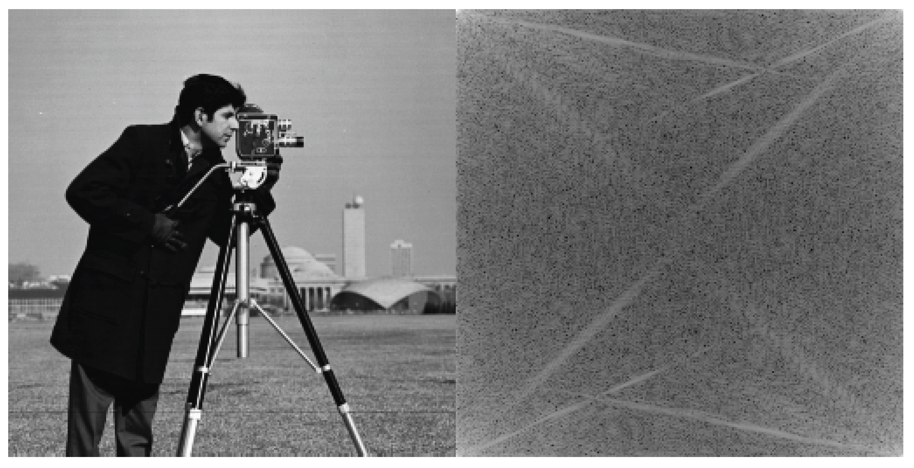
Figure 2.
(a) JPEG block diagram, (b) Pseudo-code implementing JPEG with 2D-DCT.
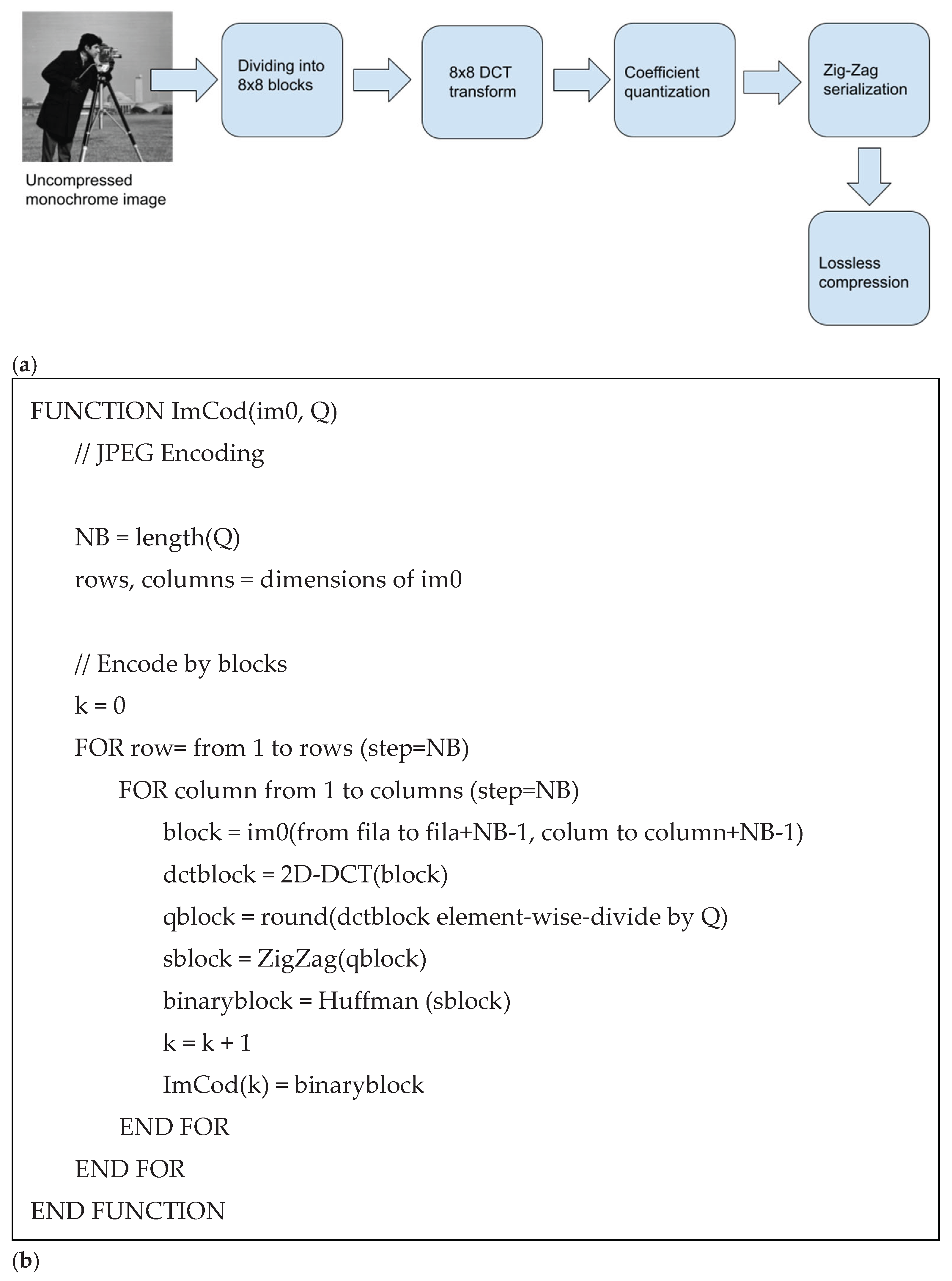
Figure 3.
Zig-zag ordering from JPEG standard.
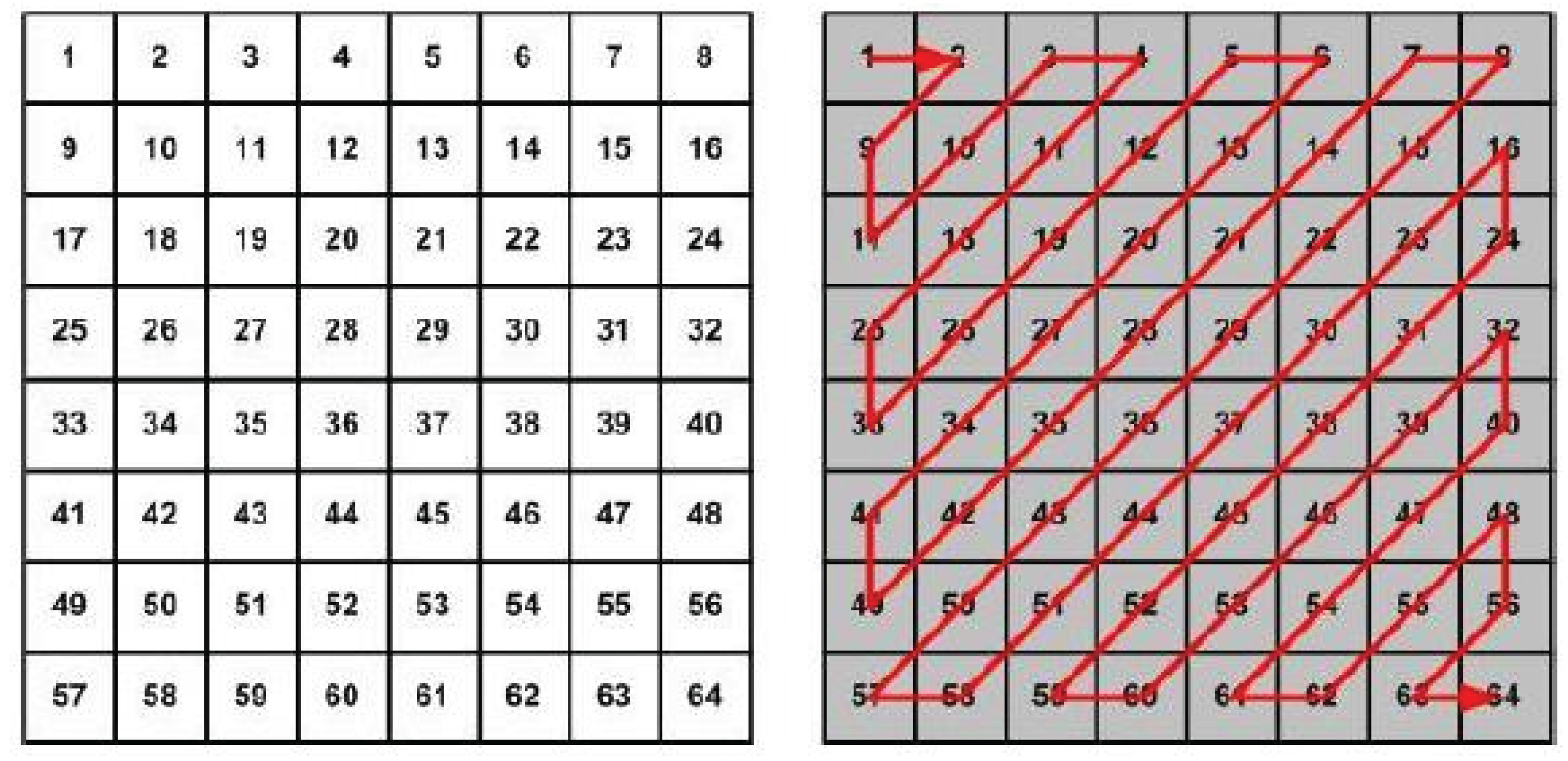
Figure 4.
(a) 3D-DCT coder block diagram, (b) Pseudo-code implementing video coding with 3D-DCT. Note that code takes into account if number of frames is not multiple of Z.
Figure 4.
(a) 3D-DCT coder block diagram, (b) Pseudo-code implementing video coding with 3D-DCT. Note that code takes into account if number of frames is not multiple of Z.
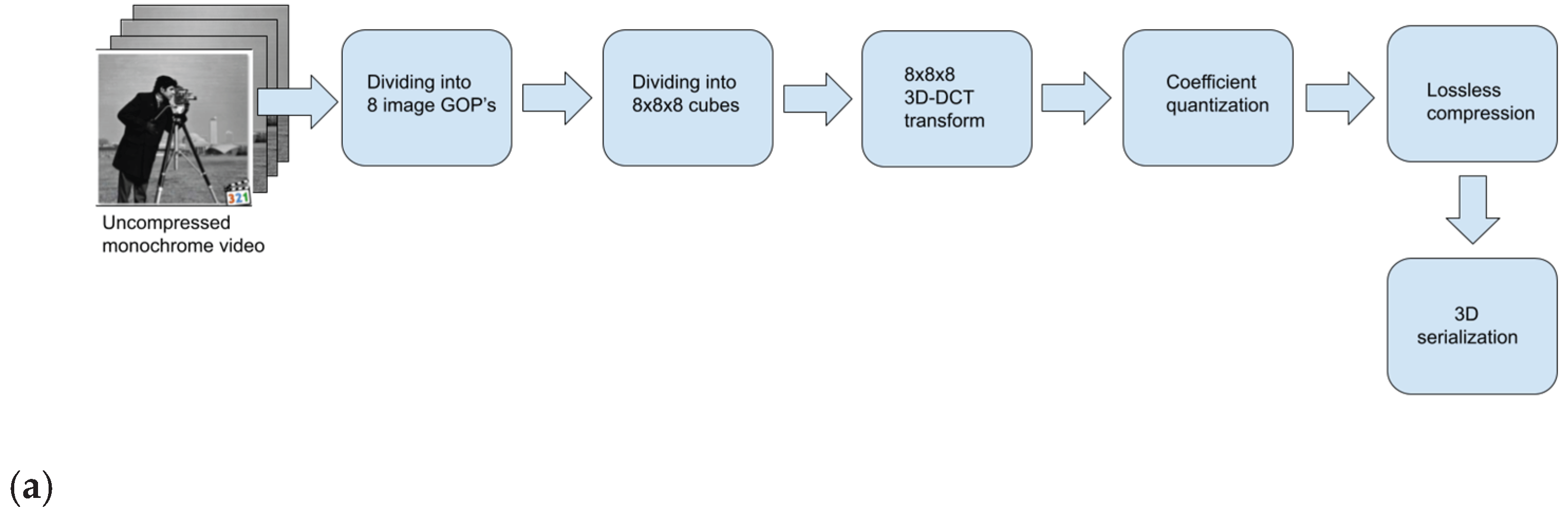
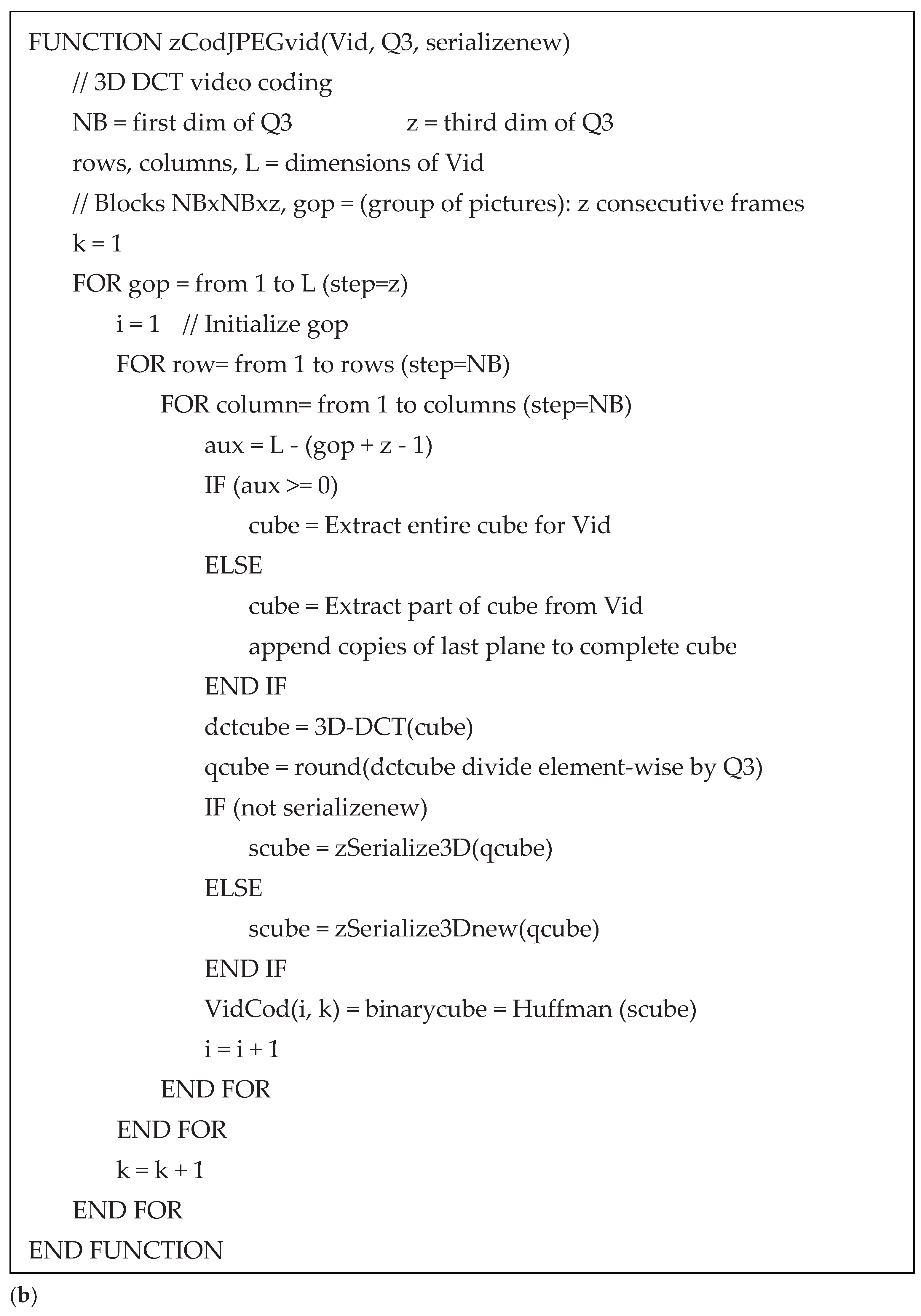
Figure 5.
Performance figures represented in a graph.
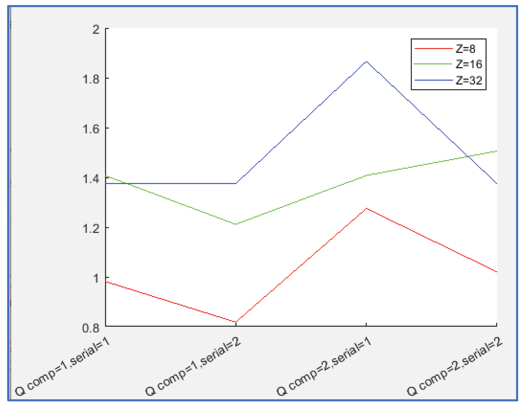
Figure 6.
Performance figures represented in a graph.
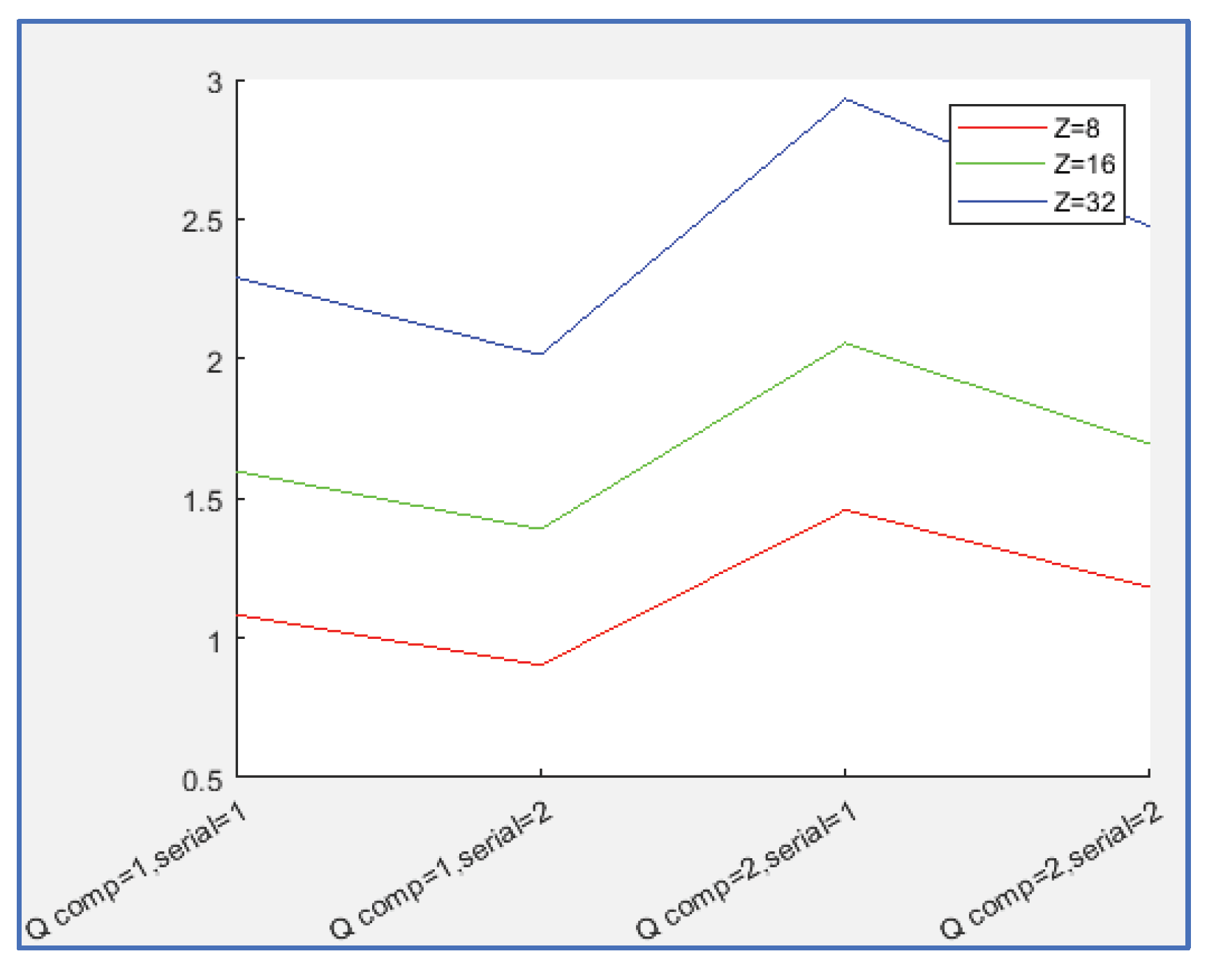
Table 1.
Full results for monochrome video.
| Coder |
Z (GOP) |
Q coefficients Computation method |
Serialization Method |
PSNR mean/std |
Compression Ratio Mean/std |
Processing time per frame |
|---|---|---|---|---|---|---|
| 3D-DCT, v0 Baseline |
8 |
1 | 1 | 37.91/1.37 | 29.50/14.93 |
0.96 |
| 3D-DCT, v1 | 8 | 1 | 2 | 37.65/1.01 | 24.53/10.71 | 0.93 |
| 3D-DCT, v2 | 8 | 2 | 1 | 37.20/1.11 | 40.36/22.73 | 0.92 |
| 3D-DCT, v3 | 8 | 2 | 2 | 37.20/1.11 | 31.90/15.71 | 0.92 |
| 3D-DCT, v4 | 16 | 1 | 1 | 37.93/1.06 | 43.38/23.41 | 0.50 |
| 3D-DCT, v5 | 16 | 1 | 2 | 38.06/1.10 | 37.39/17.58 | 0.51 |
| 3D-DCT, v6 | 16 | 2 | 1 | 37.83/1.13 | 56.88/35.79 | 0.50 |
| 3D-DCT, v7 | 16 | 2 | 2 | 37.83/1.13 | 46.47/25.25 | 0.49 |
| 3D-DCT, v8 | 32 | 1 | 1 | 38.25/1.13 | 61.79/25.24 | 0.29 |
| 3D-DCT, v9 | 32 | 1 | 2 | 38.34/1.21 | 54.01/29.16 | 0.28 |
| 3D-DCT, v10 | 32 | 2 | 1 | 38.21/1.20 | 79.09/54.74 | 0.28 |
| 3D-DCT, v11 | 32 | 2 | 2 | 38.21/1.20 | 66.16/38.65 | 0.28 |
| MPEG-4, MATLAB baseline |
90 |
NA | NA | 42.32/0.85 | 27.35/13.77 |
NA |
| H.265 (ffmpeg) | 8 | NA | NA | 37.37/1.29 | 56.37/30.45 | NA |
| H.265 (ffmpeg) | 16 | NA | NA | 37.62/1.33 | 81.21/47.34 | NA |
| H.265 (ffmpeg) | 32 | NA | NA | 37.47/1.31 | 112.81/74.73 | NA |
Table 2.
Full results for color video.
| Coder |
Z (GOP) |
Q coefficients Computation method |
Serialization Method |
PSNR mean/std |
Compression Ratio mean/std |
Processing time per frame |
|---|---|---|---|---|---|---|
| 3D-DCT, v0 Baseline |
8 | 1 | 1 | 33.34/1.29 | 77.44/36.88 | 1.38 |
| 3D-DCT, v1 | 8 | 1 | 2 | 33.00/0.64 | 65.44/25.96 | 1.37 |
| 3D-DCT, v2 | 8 | 2 | 1 | 32.69/0.74 | 105.30/55.07 | 1.36 |
| 3D-DCT, v3 | 8 | 2 | 2 | 32.69/0.74 | 84.78/37.54 | 1.36 |
| 3D-DCT, v4 | 16 | 1 | 1 | 33.42/1.18 | 115.20/59.97 | 0.74 |
| 3D-DCT, v5 | 16 | 1 | 2 | 33.16/0.69 | 100.42/43.91 | 0.73 |
| 3D-DCT, v6 | 16 | 2 | 1 | 33.00/0.74 | 149.94/89.64 | 0.73 |
| 3D-DCT, v7 | 16 | 2 | 2 | 33.00/0.74 | 123.98/62.12 | 0.72 |
| 3D-DCT, v8 | 32 | 1 | 1 | 33.17/0.75 | 164.96/98.98 | 0.42 |
| 3D-DCT, v9 | 32 | 1 | 2 | 33.20/0.77 | 145.47/74.55 | 0.41 |
| 3D-DCT, v10 | 32 | 2 | 1 | 33.22/0.99 | 210.86/141.57 | 0.41 |
| 3D-DCT, v11 | 32 | 2 | 2 | 33.12/0.77 | 177.79/98.58 | 0.41 |
| MPEG-4, MATLAB | 90 | NA | NA | 35.65/0.74 | 66.59/22.62 | NA |
| H.265 (ffmpeg) | 8 | NA | NA | 70.33/2.40 | 47.35/22.66 | NA |
| H.265 (ffmpeg) | 16 | NA | NA | 70.35/33.25 | 66.30/33.25 | NA |
| H.265 (ffmpeg) | 32 | NA | NA | 70.28/2.40 | 87.60/47.59 | NA |
Table 3.
Full results for medical CT’s.
| Coder |
Z |
Q coefficients Computation method |
Serialization Method |
PSNR mean/std |
Absolute Compression mean/std |
Relative Compression mean/std |
Processing time per frame |
|---|---|---|---|---|---|---|---|
| 3D-DCT, v0 Baseline |
8 | 1 | 1 | 37.56/3.28 | 315.63/ 236.84 |
285.56/ 237.77 |
2.38 |
| 3D-DCT, v1 | 8 | 1 | 2 | 37.56/3.28 | 356.58/ 256.54 |
319.93/ 262.03 |
2.42 |
| 3D-DCT, v2 | 8 | 2 | 1 | 36.90/2.74 | 476.84/ 358.60 |
429.74/ 356.01 |
2.46 |
| 3D-DCT, v3 | 8 | 2 | 2 | 36.90/2.74 | 521.75/ 388.11 |
466.84/ 380.16 |
2.46 |
| 3D-DCT, v4 | 16 | 1 | 1 | 36.90/3.01 | 415.63/ 307.66 |
377.13/ 311.04 |
1.27 |
| 3D-DCT, v5 | 16 | 1 | 2 | 36.90/3.02 | 523.70/ 393.39 |
472.37/ 390.77 |
1.26 |
| 3D-DCT, v6 | 16 | 2 | 1 | 36.59/2.71 | 668.22/ 517.00 |
606.13/ 516.16 |
1.26 |
| 3D-DCT, v7 | 16 | 2 | 2 | 36.59/2.71 | 819.66/ 641.15 |
739.44/ 631.14 |
1.25 |
| 3D-DCT, v8 | 32 | 1 | 1 | 36.13/2.71 | 537.49/ 394.29 |
488.48/ 401.28 |
0.73 |
| 3D-DCT, v9 | 32 | 1 | 2 | 36.13/2.71 | 726.67/ 554.28 |
659.36/ 555.27 |
0.75 |
| 3D-DCT, v10 | 32 | 2 | 1 | 36.09/2.67 | 863.22/ 676.02 |
787.82/ 679.64 |
0.75 |
| 3D-DCT, v11 | 32 | 2 | 2 | 36.09/2.67 | 1166.40/ 946.93 |
1064.40/ 943.18 |
0.71 |
Table 3.
Full results for medical MRI’s.
| Coder |
Z |
Q coefficients Computation method |
Serialization Method |
PSNR mean/std |
Absolute Compression mean/std |
Relative Compression mean/std |
Processing time per frame |
|---|---|---|---|---|---|---|---|
| 3D-DCT, v0 Baseline |
8 | 1 | 1 | 39.97/2.26 | 44.20/5.9 | 34.31/2.54 |
4 |
| 3D-DCT, v1 | 8 | 1 | 2 | 39.97/2.26 | 58.43/6.94 | 45.37/2.60 | 4 |
| 3D-DCT, v2 | 8 | 2 | 1 | 38.47/2.03 | 63.59/6.56 | 49.41/2.01 | 4 |
| 3D-DCT, v3 | 8 | 2 | 2 | 38.47/2.03 | 88.68/8.52 | 68.93/2.32 | 4 |
| 3D-DCT, v4 | 16 | 1 | 1 | 37.17/1.43 | 60.09/3.80 | 46.79/0.71 | 2.1 |
| 3D-DCT, v5 | 16 | 1 | 2 | 37.18/1.44 | 81.31/7.37 | 63.23/1.83 | 2.1 |
| 3D-DCT, v6 | 16 | 2 | 1 | 36.97/1.58 | 75.29/3.67 | 58.65/1.00 | 2 |
| 3D-DCT, v7 | 16 | 2 | 2 | 36.97/1.58 | 101.73/6.90 | 79.18/0.32 | 2.1 |
| 3D-DCT, v8 | 32 | 1 | 1 | 35.43/1.22 | 82.29/13.12 | 63.80/6.45 | 1.2 |
| 3D-DCT, v9 | 32 | 1 | 2 | 35.47/1.25 | 104.52/17.60 | 81.00/8.91 | 1.2 |
| 3D-DCT, v10 | 32 | 2 | 1 | 35.55/1.30 | 97.90/15.47 | 75.90/7.54 | 1.2 |
| 3D-DCT, v11 | 32 | 2 | 2 | 35.55/1.30 | 122.88/20.15 | 95.24/10.03 | 1.1 |
Disclaimer/Publisher’s Note: The statements, opinions and data contained in all publications are solely those of the individual author(s) and contributor(s) and not of MDPI and/or the editor(s). MDPI and/or the editor(s) disclaim responsibility for any injury to people or property resulting from any ideas, methods, instructions or products referred to in the content. |
© 2026 by the authors. Licensee MDPI, Basel, Switzerland. This article is an open access article distributed under the terms and conditions of the Creative Commons Attribution (CC BY) license (http://creativecommons.org/licenses/by/4.0/).
Copyright: This open access article is published under a Creative Commons CC BY 4.0 license, which permit the free download, distribution, and reuse, provided that the author and preprint are cited in any reuse.