
Submitted:
26 January 2026
Posted:
27 January 2026
You are already at the latest version
Preprints on COVID-19 and SARS-CoV-2
Abstract
This study examines whether excess mortality in Spain is returning to pre-pandemic levels by quantifying the increase in mortality associated with COVID-19 during the period 2020–2023. To achieve this objective, we apply a forecasting-based methodology that can be used in any regional or temporal context, relying on several stochastic mortality models to project future mortality rates using pre-pandemic data and comparing these projections with observed values. The results reveal substantial excess mortality during the pandemic years, followed by a gradual decline that suggests a partial return toward pre-pandemic mortality patterns. The analysis highlights the usefulness of multi-model stochastic approaches for evaluating the impact of mortality shocks and for monitoring the extent to which mortality normalizes after such events. The findings underscore the need for robust statistical tools to support public health assessment and to inform prevention and response strategies in future health crises.
Keywords:
excess mortality
; stochastic mortality models
; COVID-19
; epidemiology
; time-series forecasting
; Spain
1. Introduction
The COVID-19 pandemic has been an unprecedented global public health challenge. Since its appearance, the virus has affected millions of people and strained the capacity of the health systems of every country in the world. Scientific research has been fundamental to understanding the disease, developing vaccines and treatments, and putting in place prevention measures. Various studies have approached the pandemic from different perspectives, including epidemiology (Madewell, Yang, Longini, Halloran, & Dean, 2020), immunology (Arif, Ansari, Ahsan, Mahmood, & Halim Khan, 2021), forecasting (Petropoulos, Makridakis, & Stylianou, 2022) or insurance (Liu & Araz, 2024). From a management perspective, several studies analyse the strategies implemented during the pandemic, focusing on the economic impacts and highlighting the need to make decision-making more flexible in order to apply rapid planning policies that mitigate negative effects. In an era marked by overlapping crises, such as the COVID-19 pandemic and the war in Ukraine, it is relevant to take a closer look at markets centered on risk management—namely, the insurance market—in terms of their organization and future development. Waniak-Michalak (2024) examines how crises related to the COVID-19 pandemic have affected insurance business lines under dynamically changing conditions. This study is divided into three main periods of analysis: the pre-COVID-19 period, the COVID-19 period, and the COVID-19 recovery period (in which we are currently situated). The findings highlight the need for further exploration of this research area to ensure the best possible sustainable development of the insurance industry and to better prepare it for potential disruptions or crises. Complementing this work, Toppur (2023) analyses firms selling commercial vehicles and the effect of manufacturers anticipating demand to optimize production schedules. The study shows that, as life returns to normal after the financial crisis caused by COVID-19, predictive models can be strategically employed to overcome such disruptions. Therefore, impact measurement methodologies—particularly those aimed at assessing and reducing negative impacts, such as the one proposed in this paper—are highly desirable.
In this context, excess mortality has become a key indicator to assess the real impact of the pandemic, beyond the official data of COVID-19 deaths. Excess mortality is typically defined as the difference between the observed numbers of deaths in specific time periods and expected numbers of deaths in the same time periods (Centers for Control Disease and Prevention, 2023). This indicator allows the identification of the direct and indirect impact of the pandemic on mortality, being the indirect deaths those which came due to late diagnosis or lack of resources due to the pandemic emergency.
Measuring excess mortality is important for two reasons. First, it provides a more accurate picture of the real impact of the pandemic on population health, allowing health authorities and researchers to better understand the magnitude of the crisis and to make informed decisions about control and mitigation measures. Second, measuring excess mortality is essential to assess the effectiveness of policies and strategies implemented to combat the pandemic, as well as to learn valuable lessons for future public health crises. In addition to its importance for public health, excess mortality also has relevant implications for other sectors, such as the insurance and pension industries. Life insurance companies and pension schemes, for example, need to understand the impact of the pandemic on mortality in order to adjust their risk models and ensure the sustainability of their products and services.
In a wider approach, the crisis encouraged companies in the sectors of insurance, healthcare or finance to improve their strategic organizational responses, by boosting digital transformation and reviewing business continuity plans. According to (Bahmani, Bhatnagar, & Gauri, 2023), the shareholders showed a preference for firms that prioritized financial resilience over short-term social responsibility actions in the worst stages of the pandemic. These preferences show that a proactive crisis response and risk-based forecasting are increasingly essential for long-term sustainability.
The aim of this work is, then, to measure the excess of mortality caused by the pandemic. This means quantifying the difference between the expected mortality in a world without pandemic and the real one. To do this, mortality statistics for the last 30 years are obtained and projected to the years after the pandemic. In this study, we assume that there is no model capable of making predictions with full reliability, as highlighted by Schnürch et al. (2022), Schnürch (2023) and Dimai (2024), who examine the Lee–Carter family of models and identify notable limitations in their forecasting performance. To mitigate what is often referred to as “technique bias,” we adopt
a multi-model approach and select those models deemed most appropriate for the context under analysis. The projections are made using stochastic mortality models, such as Lee-Carter (Lee & Carter, 1992), CBD (Cairns, Blake, & Dowd, 2006) and Age-Period-Cohort (Columbia University Mailman School of Public Health, 2016). With this, we have the expected mortality without considering the pandemic for these last years and the projection is compared with reality using a series of indicators. These indicators help us to better understand how the pandemic has affected the mortality, the trends it follows and its future behaviour.
The data used for this article consists of the historical data of mortality of Spain for the 30 years prior to the pandemic, spanning from 1990 to 2019, and data of mortality for the 5 years after the pandemic; this is 2020 to 2024. This extensive timeframe enables the establishment of a robust foundation for analysis and comparison, facilitating the identification of long-term trends and patterns in Spanish mortality. The data was taken from the from Human Mortality Database (HMD) and the Spanish National Institute of Statistics (INE). The software used to analyse the data is R, using the StMoMo package, a specialized and highly effective tool for working with stochastic mortality models.
The response to the questions raised is a mixture of quantitative and qualitative (which is ordinal and numerical) sense. It is based on the analysis of numerical data and some indicators will determine if there was or there was not a type of excess of mortality for a specific year and age, while others will give us a quantification of that excess. With that, we can comprehend the effect of COVID-19 in the Spanish mortality and the evolution of that effect through the years.
The work is organized into different sections. In the second we give some statistical and actuarial definitions and see the historical evolution of mortality analysis. In the third section we explain the methodology, the existing models and the data and software used. In the fourth section, the data is analysed statistically and the questions raised will be answered. Finally, in the fifth section the conclusions drawn from the data will be discussed. The work is completed by the Bibliography section.
2. Background and Theoretical Framework
Apart from the own experience of the last years, studies have been done on the opinions of expert actuaries and demographers on the future behaviour of mortality. In an article about this topic, (Reynolds & Dattani, 2023, 31 de marzo) believe that, even without the virus, the steep decline in mortality that occurred during the 20th and early 21st centuries was already stagnating and would deteriorate in the coming years. The factors that explain this are, among others, climate change, population growth or wars. Not all these factors apply to Spain, but in a globalized society it seems logical that no country should be left out of these events.
In Spain, the “Instituto de Salud Carlos III” (ISCIII) is the international reference entity in Public Health and Biomedical Research. This body prepares the report Excess of mortality identified by the Daily Mortality Monitoring System (MoMo) (ISCIII, 2018), which tries to identify the deviations of daily mortality observed with respect to that expected according to the historical mortality series and allows to indirectly estimate the impact of any event of importance in Public Health.
According to this report, and as shown in Figure 1, the total death rate in Spain has been increasing steadily until 2019, with the slight fluctuations inherent in a process of a stochastic nature. This increase is explained by increase of weight of the population of the most advanced age groups respect to the total population, groups in which the baby boom generation is already immersed, a phenomenon known as the “inversion of the population pyramid” (Fundación MAPFRE, 2022). This phenomenon is also visible in other European countries (Directorate-General for Economic and Financial Affairs, 2023). However, in 2020, the year in which the pandemic emerges, we see a sharp increase in mortality that is not explained by the trends up to that point and, therefore, is attributable to the effects of COVID-19.
The “Instituto Carlos III” annually monitors daily excess of mortality (initially caused by climate change, although it now measures excesses due to any cause) through the Daily Mortality Monitoring System (MoMo). The report (ISCIII, 2018) defines various indicators of excess mortality, which have statistical nature and are measures that attempt to scientifically quantify a characteristic of a sample. Some indicators are qualitative, and others are quantitative. An alert is reported when the number of deaths observed is above the number expected in the analysis period. There are different types of alerts, depending on the degree of difference between expected and actual mortality. An excess of mortality occurs when the observed number of daily deaths exceeds the upper limit of the 99% confidence interval for the expected number of daily deaths. The MoMo defines some quantitative indicators, such as the excess of deaths which is the difference between the number of observed deaths and the number of expected deaths during the period considered of “excess of mortality”. Another quantitative indicator is the percentage of excess of deaths.
Because the indicators are general and objective, it is possible to have a clear idea of whether an excess of mortality is occurring in a period or not, while at the same time standardizing their analysis to facilitate comparison between periods or regions. We can also have a quantitative sight of the excess in each period.
2.1. Data and Methods
In this paper we seek to quantify the effect of COVID-19 on mortality in Spain, since, as we have pointed out in section 2.1, there has been a notable increase in mortality. To do this we project mortality rates for the last 30 years with different stochastic models and see what values would be expected for the period 2020-2025. We use the actual data for these years to compare them, analysing the differences observed using the indicators defined for this purpose.
2.2. Stochastic Mortality Models
Stochastic mortality models are used to characterize the evolution of mortality and thus facilitate its study over time. In this work we characterize mortality rates in order to make projections of these rates according to age, period or cohort. In this section we briefly describe some of the most relevant models and their characteristics. It is usual for these models to consider that the mortality phenomenon is distributed as a random variable with Poisson or Binomial law, by age.
- ▪
- Lee-Carter model
In 1992, the statisticians Ronald Lee and Lawrence Carter (Lee & Carter, 1992) proposed a model to project the mortality rate that differs from other models in that it assumes no cap on life expectancy, but allows age-specific mortality to decrease without limit. This method is one of the most widely used and is based on the following expression, where x is the age-related subscript and t is the year-related subscript:
In order to correctly estimate the parameters, it is necessary to apply some restrictions, such as:
The Lee-Carter model is one of the most widely used in the actuarial world (Cairns, Blake, & Dowd, 2008 (2-3)), (Lee & Miller, 2001) and since its publication different variants have emerged, as well as multiple applications. For example, the Lee-Carter model was adapted to explain the influence of climate on mortality (Boumezoued, Elfassihi, Germain, & Titon, 2022). The (Hyndman & Ullah, 2007) functional mortality model is an extension of the Lee-Carter which allows for smooth functions of age and the amount of noise to become age-specific. Another Lee-Carter adaptation is the (Renshaw & Haberman, 2006) model, which is a cohort-based model that incorporates a cohort effect to the Lee-Carter predictor to better capture discontinuities in mortality trends.
- ▪
- Cairns-Blake Dowd (CBD)
This model (Cairns, Blake, & Dowd, 2006), which differs from the others in that it does not require restrictions on the parameters. In this model the authors assume a binomial distribution for mortality, so the model is expressed with the following equation:
As stated in (Díaz Rojo, 2021), this model assumes the mortality is linear in the logit scale. Consequently, it only works well for older ages, leading to high residuals in early ages and a poor behaviour in general for the residuals. In (Cairns A. J., y otros, 2009) we find a generalization of the CBD model suggesting that the impact of the cohort effect on a specific cohort decreases over time.
- ▪
- Age-Period-Cohort (APC)
This model (Columbia University Mailman School of Public Health, 2016) considers these three variables (age, period, and cohort) as the determinants of variation in mortality rates in a population. This is the key difference with the other models, although extensions and variations of the Lee-Carter and the CBD have also incorporated these elements. We see the role of each one:
- Age: Collects the variations inherent to biological age and the social processes associated with each age.
- Period: It includes the external effects derived from the historical period in which the population is found. It therefore affects everyone equally. An example of a period effect can be wars, droughts, politics or environmental changes.
- Cohort: These are variations that affect only a cohort born in a given period. Therefore, the determining variable here is the year of birth. This can be influential in the case of an epidemic affecting only children during a period or a child vaccination program.
Since the Cohort variable can be obtained as “Period” minus “Age”, a linear dependence arises between the variables that gives rise to what is known as the “Identification Problem”: the difficulty of correctly and independently estimating the effect of each of the three variables. The solution is, for example, to use restrictions on the values of the predictors, as in the Lee-Carter model.
The formulation of this model is as follows:
The restrictions to avoid the identification problem are analogous to those of Lee-Carter:
To avoid the technique bias, we will test the Lee-Carter, the CBD and the APC models in the data and compare the results to ensure the best model for our data is used.
2.3. Goodness of the Models
One of the most commonly used statistical tools to assess the quality of a model are the information criteria. When models have many possible explanatory variables, as is the case of a mortality model (the variables would be all the ages of each observed year), it is necessary to limit the number of these, as too many can add a lot of noise and complexity to the model. At the same time, the model must be reliable and have quality predictors that return a good fit. These information criteria allow us to quantify the balance between predictive capacity and complexity as follows:
The two main criteria are the Akaike Information Criterion (Akaike, 1980) and the Bayesian Information Criterion (Schwarz, 1978). Their mathematical expressions are the following:
where k expresses the number of model parameters and L the value of the maximum of the likelihood function of the data.
where n is the size of the sample.
Another useful indicator of the goodness of the model is the deviance, which is a quality-of-fit statistic for a model that is often used for statistical hypothesis testing. A lower deviance means a better fit to the data.
Procedure
Now, we describe how to determine which models adequately measure excess mortality and can therefore be used in this study. The following process has been structured with for this purpose. First, the period for which data is available is divided into subperiods of similar size, [, ]. Second, for each subperiod, a mortality rate prediction is made for each age with a forecast horizon of h=5, 10 or 20 years. Third, the predicted mortality rate for each age () is compared with the actual observed values (), which were not used in the prediction. To assess the adequacy of the models, the mean squared error is considered as the evaluation metric. The sum of these errors, across all considered ages and for all years that make up the validation period (5, 10, or 20 years), constitutes the model’s indicator, which is summarized in (10).
Where is named the h-Quadratic mean square error; and is the known actuarial infinity.
The models are ordered using the indicator and the best model to our purpose is the model with the lowest value in this indicator.
2.4. Excess of Mortality Indicators
In Section 2 we show some indicators that the ISCIII uses to measure the impact on Spanish mortality, initially due to climate change. These focus on the daily evolution of mortality by territory, measuring daily confidence intervals or differences between expected deaths and reality.
The objective of our analysis is different, and we cannot use this type of indicators directly. We therefore made an adaptation of the indicators used by the ISCIII in its MoMo report to adapt them to annual mortality broken down by age group as indicated below.
We consider the following indicators to measure the exceed of mortality for each age.
Firstly, the Punctual excess mortality (PEM), we said that an arbitrary age has a PEM when the mortality rate for this age is higher than the expected value. Then, we consider the Relative excess mortality (REM) the percentage by which the actual mortality rate exceeds the expected value. Finally, if the mortality rate for an arbitrary age exceeds the upper limit of the 99% confidence interval of the mortality prediction for that particular age, we said that this age has an Excess of mortality (EM).
The mechanism we built to perform the calculations considers the following guidelines:
The main target is to forecast the mortality for the years 2020 to 2025 (estimated data) with the information observed until 2019. Therefore, the forecast horizon is variable, going from 1 to 6 years. To guarantee the reliability of our results, the validation must be made with data forecasted with such horizons.
To perform these validations, the years 2000 to 2019 are forecasted with horizons of 1 to 6 years, what will lead us to compare the results of the year 2020 with the predictions done with a horizon of 1 year; the results of the year 2021 with the predictions done with a horizon of 2 years, etc.
Finally, the results are grouped into 10-year age groups; the mortality indicators of each group will be analysed according to the number of indicators by age that have occurred in each group.
2.5. About the Data
Human Mortality Data Base (Human Mortality Database (HMD), s.f.) and INE (Instituto Nacional de Estadística (INE), s.f.) provide us the mortality rates. In particular, the data used in this study are referred to Spain, in period from 1990 to 2025 (estimated data), and for ages in 0 to 100 years. The databases consist of two matrices, one with the exposed population by age and year of calendar, and another with the number of deaths by age and year. Both set of data have been obtained from the Human Mortality Database (Human Mortality Database (HMD), s.f.), which in turn is obtained from the respective national statistical institutes of each country. The data for 2022 and 2023 were obtained directly from the INE (Instituto Nacional de Estadística (INE), s.f.), since they were not yet included in the HMD. The data for 2024 and 2025 is also from the INE, but it is an estimation since official data is not available yet.
2.6. Software and Packages
For data analysis we use R-Studio (Posit Team, 2023) (Version 1.2.5001) and, in particular, the StMoMo package (Villegas, Kaishev, & Millossovich, 2018), which includes tools for implementing generalized stochastic mortality models such as those we have seen in previous chapters (Lee-Carter, APC, CBD). It includes functions for fitting mortality models, analysing goodness-of-fit, and performing mortality predictions and simulations. The demography package (Hyndman, 2023) has also been used for downloading HMD data. The data and the script developed to the process, the validation step, the estimation of the h-Quadratic mean square error, and to determine the best model, are available in (Ibáñez & Morillas, 2025).
3. Results
In this section we derive the main result of the investigation. We apply the models described before to mortality data from Spain in the period prior to the pandemic. We describe the mortality situation and analyse the mortality excesses of reality with respect to the predictions of the models using the indicators defined, which help us to characterize the excess of mortality derived from the COVID-19 pandemic.
3.1. Descriptive Analysis
Mortality in Spain is shown for the years of the pandemic, that is 2019 to 2023. We can observe the logarithmic mortality rates before the COVID-19 appeared and its evolution through the time.
The shape of the mortality rates curves we see in the left panel of Figure 2 is the usual for a country like Spain. This shape can be structured as follows: there is a first stage considered (i) adaptation to the environment, which represents infant mortality in the first years of life, from birth onwards the mortality rate falls until 4-7 years of age, when it begins to rise. At the end of the first stage, two overlapping stages begin: (ii) natural mortality, which lasts until the oldest ages, 80 years and older; and (iii) the social hump, also known as the accident hump. This hump is a bulge that occurs at the end of the first stage and can have variations both in amplitude and in the age at which the maximum risk occurs. In this case, the amplitude is from age 17 to 30, with a maximum at age 22. It can be seen that the mortality rate referred to natural longevity is a steadily increasing but stable curve until approaching actuarial infinity.
The evolution of the curves shows high volatility for the lower ages, and in the right panel we can start noticing lower values for the year 2019 respect to the other years. This goes on until the age of 45, where the year 2023 will continue, until the actuarial infinity, being the year with the lowest mortality, meaning the effects of the pandemic are almost gone. From the age of 45, the year 2020 is the one with highest mortality, showing the big impact in the middle aged and elder population.
From the age of 50, the curves show very little volatility and do not intersect, each one following its path with different levels of mortality.
From these figures we get a global view of the mortality rates, but the analysis of excess mortality cannot be rigorously performed based on the raw data. For this reason, the articulated process involves applying the previously introduced dynamic mortality models to predict an expected value in a non-pandemic scenario and then comparing them with the observed values and, via the quantitative measures defined to characterize excess mortality, making a more accurate interpretation, as correct as possible. The models selected are Lee-Carter, APC and CBD.
3.2. Model Fitting and Selection for Prediction
To determine the suitability of the models introduced and thus take into consideration the one or another model, we use the information criteria introduced in Section 4.4, the AIC and the BIC, as well as the deviance.
Table 1 allows us to ensure that the model that provides the most information for the set of all ages in relation to the available data is the APC. It is this model that has the lowest values in the two information measures considered, AIC and BIC and in the deviance. The left panel of Table 1 shows the values for the models considering all ages.
It is important to note the difference in magnitude between the models. While the Lee-Carter and APC models have similar magnitudes, the CBD model presents values within the order of 20 times bigger than the other models. According to Diaz Rojo (Díaz Rojo, 2021) this happens because the CBD model is linear in both logit and log scale; it is usually indicated that this is because this model does not characterize well the adaptation to the environment or the fluctuations of the social hump, so it can be verified that it will work better at older ages. Thus, the panel 2 collects the AIC and BIC values only for ages 70 to 100 years.
Note that, although the best models are still APC and Lee-Carter, now the magnitude of the AIC and BIC values has been reduced to only 50% more for CBD, as opposed to the set for all ages, whose value was in the neighbourhood of 2000%.
Once this is resolved, the conclusions provided by the information criteria is that for both age ranges, it is the APC model that has the highest quality, closely followed by the Lee-Carter. The CBD, despite improving when only older ages are considered, continues to be the worst performer according to the AIC and BIC information criteria. In this sense, both Lee-Carter and APC are good candidates to use in our predictions.
Regarding the residuals of the models, the CBD shows clear patterns influenced by the linearity of the model observed previously. Thus, up to 40 years of age, a clear over mortality is detected, due to the fact that the model does not correctly reflect the low juvenile mortality. The APC and Lee-Carter show some patterns for some cohorts, but these are not so clear.
The BIC and AIC information criteria do not allow us to differentiate between the Lee-Carter and APC models; they can have similar values for these indicators and, at the same time, not predict well for some ages. To determine whether one or the other model predicts better at certain ages, we use a measure of precision such as the quadratic error. Thus, we use the expression (11) for different years of the period.
In the case of the Lee-Carter model, for a prediction time horizon of 5 years we take data from the period 1990-2010. With these data the model is adjusted, and this adjustment is used to predict the following 5 years, from 2011 to 2015. With the values of the predictions made and the observed values for the same years, the quadratic errors of prediction are obtained:
This would be repeated several times, advancing each time by one year, both in the adjustment interval and in the prediction period, without overlapping (in the second prediction the data used are those of the years 1991-2011, and the projection is made for the years 2012-2016). This makes it possible to quantify the predictive capacity of each model. Applying this process also to the APC and CBD method allows us to select the model to be used in the estimation of excess mortality caused by COVID-19.
As we can see, for short and medium-term projections, Lee-Carter is the best performing model. However, for a long-term projection, the CBD model appears as the best model, although very close to Lee-Carter. Based on these indicators, taking into consideration not only the mean square error but also the values of AIC and BIC and the prediction time horizon for excess mortality estimates (4 years), we determine that Lee-Carter is adequate to perform the analysis.

Table 2.
Quadratic error of the models.
| Years of prediction | LC | CBD | APC |
|---|---|---|---|
| 5 | 0.2093 | 1.6655 | 0.473 |
| 10 | 0.6369 | 2.7291 | 1.008 |
| 20 | 8.5337 | 7.9965 | 13.0063 |
| Source: Compiled by the authors. Data for years 2024 and 2025 are projections. | |||
3.3. Excess of Mortality Indicators
In order to accurately determine the excess of mortality that has occurred in each age group, a projection of the models is made for the years 2020 to 2025. These predictions are compared with the actual data on mortality rates and the indicators defined in section 3.3 are evaluated. Note that the maximum number of ages with an indicator is 100 for the full year and 10 for the decadal group.
First, we encounter the punctual excess mortality (PEM), any excess of the actual mortality rate over the one predicted by the projection. In Figure 3 we see the evolution of the number of PEM for every horizon. The years 2015 to 2019 show an increase in the number of indicators, with around 65% of ages having an increase in the mortality respect to what the models forecasted. In the years 2020 to 2022, this figure reaches an 85%. We can observe that in 2023 the PEM returns to the values of the years before the pandemic.
Using the Lee-Carter model to analyse the PEM by 10-year age groups, the punctual excess mortality is shown in Table 3.
When broken down by age groups, the 3 models considered provide similar values that we interpret as the “harvest effect”. For example, via the Lee-Carter model, in the years 2020 to 2022, for ages 81 to 100 years there are point excesses of mortality at almost all ages. However, in 2023, this value drops to 2. This could be explained because the first wave of the pandemic was excessively lethal, so that all the people who “probably” would have died during the first two years died along with those who might have survived for one or two more years.
We can also observe a higher excess of mortality in 2022 than in 2021. After a lethal period in 2020, there might have been a general harvest effect, so the mortality fell in 2021, but the new varieties of the virus and the “low” mortality in 2021 made the population vulnerable again and the mortality rose again in 2022. In 2023 we can observe a big drop, returning to the number of PEM of the years before the pandemic.
Figure 4 shows the excess mortality (EM) -defined as the excess of the actual mortality rate over the upper limit of the 99% confidence interval of the prediction- and the values obtained for the Lee-Carter model. We can see the evolution of the number of EM for every horizon, showing that 2020 and 2021 have a big difference respect to the usual number of EM for the years before the pandemic. Contrary to what happened in the PEM, here 2022 shows little difference with the other years, while 2023, despite having less EM, shows a big difference with the previous years.
If we group the results by decadal age groups, the results are shown in Table 4 for the Lee-Carter model.
Broken down by age and focusing on the Lee-Carter model, in the 21-40 age bracket, EMP occur at almost all ages. The intermediate ages between young adults and the elderly suffer fewer excesses, but from the age of 61 onwards they occur again at all ages in 2020. We can see a strong decrease in the number of EM for these ages that can be explained by the harvest effect, leading to almost no EM at all in 2021 for the segment of 81 to 100. In 2022 we see some EM again and in 2023 there are no EM for the ages 71 to 100.
Another important indicator of excess mortality is the relative excesses mortality (REM) of reality over that expected by the model.
Table 5 shows the REM by age group. The biggest impact occurs in the range of 21 to 40. This can be explained because their mortality in stable conditions is very low, therefore a small number of deaths in these age groups will cause a shock in their mortality rates. As stated in the other indicators, the harvest effect can be seen here, since the REM of the population aged 81 to 100 drops in 2021 and, although it raises in 2022, it drops again in 2023. It shows that all weak elderly people died in 2020, and the survivors were in better health and could resist better the virus.
3.4. Graphical Method
Following the method shown in (Navarro & Requena, 2023), now we analyse the relative excess mortality from two points of view. One is the REM as we saw it in the indicators; that is, comparing the real mortality rates with the expected ones from the Lee-Carter model. Since the data of every year is very volatile, we used the method of the simple moving average to smooth the function.
Figure 5.
REM by year.
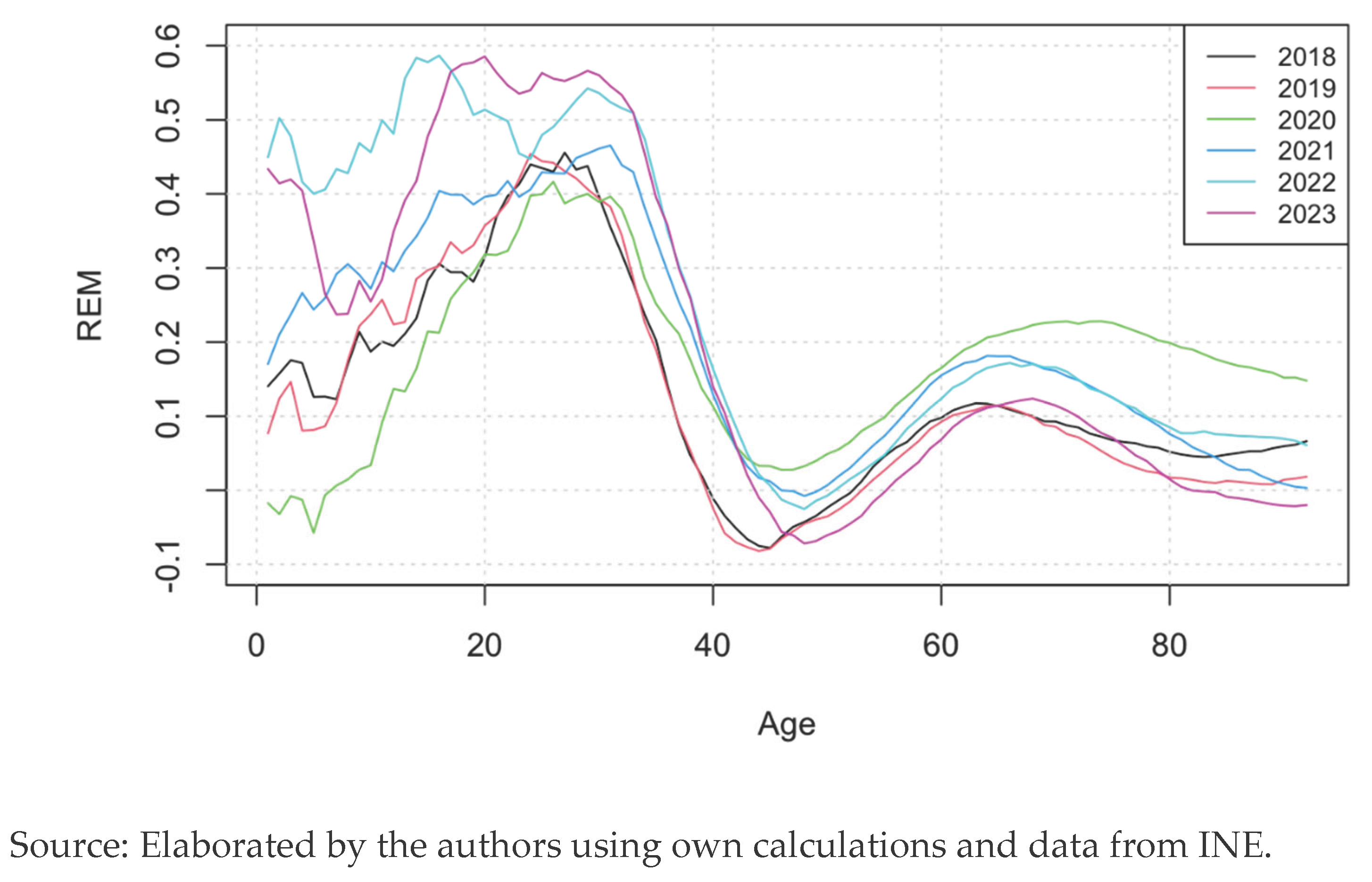
We can see that even for the years before the pandemic (2018 and 2019), the younger ages have a very high REM. That means the model undervalues the mortality for that range of ages and for those years, leading to an alleged over mortality. We observe a clear high REM in 2020 for the elderly people which then decreases until getting to normal levels in 2023. 2020 is the year with the highest REM from the age of 43 onwards.
For the ages 10 to 35 there is large increase in the REM in 2022 and 2023. This may be explained by three reasons: the first is the low mortality rate in this age range, which leads to big percentual increases in response to a small number of deaths. The second reason is that, because people were at home in 2020 and did not travel much in 2020 and 2021, the accident hump was not present in these years and in 2022 and 2023 it appeared again. The third reason, especially for 2022, is that the vaccines arrived first for the older generations and later for the younger and healthier people, so in 2022 there were two different populations in terms of protection against the virus: one vaccinated and the other non-vaccinated. For every year, there is a big drop in the REM between the ages 40 to 60.
The other point of view to analyse the relative excess of mortality is to compare every year with the precedent year. We can see this in the Figure 6.
In this analysis, we focus on the age range from 20 to 100 years. The year 2020 shows a high excess respect 2019. This makes sense, since it is the year when the virus appeared, what caused a big shock in the mortality. For the rest of the years, only 2022 has an excess of mortality, after a 2021 with a large decrease in the mortality for that age range. Looking now at the younger generations, 2021 and 2022 emerge as the years with the highest excess. That means that, after a year of big excess in 2021, the mortality increased again among the population aged 0 to 20. This huge increase caused a big decrease in 2023, when mortality rates came back to normality.
4. Discussion
Authors should discuss the results and how they can be interpreted from the perspective of previous studies and of the working hypotheses. The findings and their implications should be discussed in the broadest context possible. Future research directions may also be highlighted.
5. Conclusions
The goal of this study is to quantify excess mortality during the COVID-19 pandemic, analyse its evolution over time, and assess whether mortality in Spain is returning to pre-pandemic levels. To do this we articulate a multi-model stochastic framework, the analysis provides a detailed view of age-specific mortality patterns and offers an evaluation of how the pandemic altered the long-term trajectory of Spanish mortality. Throughout the research, various indicators were constructed to measure excess mortality, both quantitative and qualitative.
The findings suggest that, at the population level, COVID-19 mortality in Spain has transitioned from an acute shock to a post-pandemic phase characterized by a return to pre-COVID mortality patterns, consistent with a normalization of epidemiological risk.
The results show that excess mortality was not evenly distributed across the population. The indicators proposed allowed for a detailed analysis of the phenomenon, capturing variations over time and between different population groups. During the first years of the pandemic, excess mortality was strongly concentrated among older age groups, reflecting the high vulnerability of these cohorts to COVID-19. In contrast, during the later years, especially in 2022, younger cohorts displayed relatively higher excess mortality than older adults. This shift reflects changes in exposure patterns, the restoration of social mobility and the accident or social hump, and delays in medical care accumulated during the pandemic period.
The key question of this study is whether excess mortality is returning to pre-pandemic levels, and it requires an answer with distinctions. The substantial decline in excess mortality observed in 2023 indicates that Spain is indeed moving back toward baseline mortality patterns. However, this normalization is not homogeneous across age groups. Older adults exhibit a clearer return to pre-pandemic levels, in part due to a pronounced harvest effect, while younger cohorts show more persistent deviations.
The multi-model approach confirms that model choice is critical for assessing mortality shocks. The Lee-Carter model offered the best short-term predictive capacity, while APC and CBD captured long-term structure differently. The construction of quantitative and qualitative indicators enabled a refined characterization of excess mortality, revealing the heterogeneity of the pandemic’s impact and supporting the interpretation of 2023 as the first year of near-normal mortality after the pandemic shock.
From a health-economics perspective, these findings highlight the importance of incorporating stochastic mortality models into crisis assessment and long-term planning. Mortality shocks propagate differently across age groups, affecting pension liabilities, insurance pricing, and healthcare decision-making.
Limitations
This study is not without limitations, and these should be taken into account when interpreting the results. Mortality data for the most recent years (2024–2025) are still provisional and may be revised, which introduces uncertainty into the assessment of whether mortality is returning to pre-pandemic levels. The models used assume continuity in pre-pandemic mortality trends, potentially overlooking structural changes in behaviour, healthcare access, and population health conditions that may have arisen during or after the pandemic. In addition, the analysis relies on all-cause mortality and does not allow for distinguishing whether specific causes of death have returned to their pre-pandemic bhaviour, a factor that could offer relevant insights into the nature of the observed deviations. The harvest effect, while clearly observable in aggregated data, cannot be precisely quantified without individual-level longitudinal information. Finally, the stochastic mortality models employed do not incorporate socioeconomic or behavioural covariates that may influence differences in the pace at which various demographic groups return to baseline mortality levels.
Improvements
Future research could further explore several aspects arising from this study. A natural extension would be to examine cause-specific mortality to determine whether the patterns identified at the aggregate level also manifest within specific categories of death, providing deeper insight into how different components of mortality have evolved in relation to pre-pandemic levels. Additional work could analyse heterogeneity across regions, socioeconomic groups, and clinical profiles, offering a more granular understanding of the differentiated recovery of mortality patterns. Comparisons with other European countries could help contextualize Spain’s trajectory within wider demographic responses to the pandemic. Methodologically, future studies could develop structural stochastic mortality models that explicitly incorporate pandemic-induced shocks, potentially enhancing the accuracy of long-term projections. Finally, further research could evaluate how the gradual normalization of mortality affects pension systems, life-insurance pricing, and healthcare resource planning in the medium and long term. This section is not mandatory but can be added to the manuscript if the discussion is unusually long or complex.
Data Availability Statement
We encourage all authors of articles published in MDPI journals to share their research data. In this section, please provide details regarding where data supporting reported results can be found, including links to publicly archived datasets analyzed or generated during the study. Where no new data were created, or where data is unavailable due to privacy or ethical restrictions, a statement is still required. Suggested Data Availability Statements are available in section “MDPI Research Data Policies” at https://www.mdpi.com/ethics.
Conflict of interest
The authors declare that there are no conflicts of interest.
Acknowledgements and Fundings
The authors wish to state that there are no acknowledgements to declare for this work, also, this research did not receive any grant from funding agencies in the public, commercial, or not-for-profit sectors.
References
- Akaike, H. (1980). Likelihood and the Bayes procedure. Trabajos de Estadistica Y de Investigacion Operativa, 31(1), 143-166. [CrossRef]
- Arif, A., Ansari, S., Ahsan, H., Mahmood, R., & Halim Khan, F. (2021). An overview of Covid-19 pandemic: immunology and pharmacology. Journal of immunoassay & immunochemistry, 42(5), 493–512. [CrossRef]
- Ayuso, M., Corrales, H., Guillen, M., Pérez Marín, A. M., & Rojo, J. L. (2007). Estadística Actuarial Vida. Barcelona: Publicacions i Edicions de la Universitat de Barcelona.
- Bahmani, N., Bhatnagar, A., & Gauri, D. (2023). Firms’ responses to a black swan macro-crisis: Should they be socially responsible or fiscally conservative? Journal of Business Research, 161, 113783. [CrossRef]
- Boumezoued, A., Elfassihi, A., Germain, V., & Titon, E.-E. (2022, December 19). Modelling the impact of climate risks on mortality. [White Paper]. Milliman, https://www.milliman.com/en/insight/modeling-the- impact-of-climate-risks-on-mortality.
- Cairns, A. J., Blake, D., & Dowd, K. (2008 (2-3)). Modelling and management of mortality risk: a review. Scandinavian Actuarial Journal, 79-113. [CrossRef]
- Cairns, A. J., Blake, D., Dowd, K., Coughlan, G. D., Epstein, D., Ong, A., & Balevich, I. (2009). A quantitative comparison of stochastic mortality models using data from England and Wales and the United States. North American Actuarial Journal, 13(1), 1-35. [CrossRef]
- Cairns, A., Blake, D., & Dowd, K. (2006). A Two-Factor Model for Stochastic Mortality with Parameter Uncertainty: Theory and Calibration. The Journal of Risk and Insurance, 73(4), 687-718. [CrossRef]
- Centers for Control Disease and Prevention. (2023, March 8). Excess deaths associated with COVID-19. (National Center for Health Statistics) Retrieved from https://www.cdc.gov/nchs/nvss/vsrr/covid19/excess_deaths.htm.
- Columbia University Mailman School of Public Health. (2016). Age-Period-Cohort Analysis. Retrieved from https://www.publichealth.columbia.edu/research/population-health-methods/age-period-cohort-analysis.
- Ibáñez-Soriano, J. and Morillas-Jurado, F. G. (2025). Data and R-Script used to Analyze the effect of COVID-19 in the mortality of Spain with stochastic models. Zenodo [on-line: https://zenodo.org/records/17347977]. [CrossRef]
- Díaz Rojo, G. (2021). Ajuste y predicción de la mortalidad. Aplicación a Colombia. [Doctoral dissertation, Universitat Politècnica de València], https://doi.org/10.4995/Thesis/10251/171096.
- Dimai, M. (2024) Modeling and forecasting mortality with economic, environmental and lifestyle variables. Decisions Econ Finan. [CrossRef]
- Directorate-General for Economic and Financial Affairs. (2023). 2024 Ageing Report. Underlying Assumptions and Projection Methodologies. Retrieved from https://economy- finance.ec.europa.eu/publications/2024-ageing-report-underlying-assumptions-and-projection- methodologies_en.
- Fundación MAPFRE. (2022). La evolución de la pirámide invertida. Retrieved from Ageingnomics - Fundación MAPFRE: https://ageingnomics.fundacionmapfre.org/blog/evolucion-piramide-invertida/.
- Glei, D. A., Gómez Redondo, R., Argüeso, A., & Canudas-Romo, V. (2022). About mortality data for Spain. Retrieved from https://www.mortality.org/File/GetDocument/hmd.v6/ESP/Public/InputDB/ESPcom.pdf.
- Human Mortality Database (HMD). (n.d.). Human Mortality Database. Retrieved from https://www.mortality.org/.
- Hyndman, R. J. (2023). demography: Forecasting Mortality, Fertility, Migration and Population Data (R package version 1.24). Retrieved from https://pkg.robjhyndman.com/demography/.
- Hyndman, R. J., & Ullah, M. S. (2007). Robust forecasting of mortality and fertility rates: A functional data approach. Computational Statistics and Data Analysis 51(10), 4942–4956. [CrossRef]
- Instituto Nacional de Estadística (INE). (2020). Edad Media de la Población por provincia, según sexo. Retrieved from https://www.ine.es/jaxiT3/Tabla.htm?t=3199&L=0.
- Instituto Nacional de Estadística (INE). (n.d.). Mortalidad. Movimiento natural de la población. Retrieved from www.ine.es: https://www.ine.es/dyngs/INEbase/es/operacion.htm?c=Estadistica_C&cid=1254736177004&menu=ultiDatos&idp=1254735573002.
- Instituto Nacional de Estadística (INE). (n.d.). Tablas de mortalidad. Retrieved from www.ine.es: https://www.ine.es/dyngs/INEbase/es/operacion.htm?c=Estadistica_C&cid=1254736177004&menu=ultiDatos&idp=1254735573002.
- ISCIII. (2018). Excesos de mortalidad identificados por el Sistema de Monitorización de la Mortalidad Diaria (MoMo). Epidemiological National Center of Spain. Obtenido de https://cne.isciii.es/documents/d/cne/informe_momo_plan_de_calor2016_final.
- Lee, R. D., & Carter, L. (1992). Modeling and forecasting U.S. mortality. Journal of the American Statistical Association, 87(419), 659-671. [CrossRef]
- Lee, R. D., & Miller, T. (2001). Evaluating the performance of the Lee-Carter method for forecasting mortality. Demography, 38(4), 537-549. [CrossRef]
- Liu, Y., & Araz, Ö. M. (2024). Estimating the Role of Uninsured in the Spread of COVID-19 via Geospatial Bayesian Models. North American Actuarial Journal, 29(1), 199-223. [CrossRef]
- Madewell, Z. J., Yang, Y., Longini, I. M., Halloran, M., & Dean, N. E. (2020). Household Transmission of SARS-CoV-2: A Systematic Review and Meta-analysis. JAMA Network Open, 3(12), e2031756. [CrossRef]
- Navarro, E., & Requena, P. (2023). Impact of COVID-19 on Spanish mortality rates in 2020 by age and sex. Journal of Public Health, 45(3), 577–583. [CrossRef]
- Petropoulos, F., Makridakis, S., & Stylianou, N. (2022). COVID-19: Forecasting confirmed cases and deaths with a simple time series model. International Journal of Forecasting, 38(2), 439-452. [CrossRef]
- Posit Team. (2023). RStudio: Integrated Development Environment for R. Posit, PBC. Retrieved from http://www.posit.co/.
- Renshaw, A. E., & Haberman, S. (2006). A cohort-based extension to the Lee–Carter model for mortality reduction factors. Insurance: Mathematics and Economics, 38(3), 556-570. [CrossRef]
- Reynolds, C., & Dattani, A. (2023, 31 de marzo). What if mortality stops improving? Introducing a product idea that shares the risks and benefits of changes in mortality rates. Mill. Milliman, https://www.milliman.com/en/insight/what-if-mortality-stops-improving.
- Schnürch, S., Kleinow, T., Korn, R., & Wagner, A. (2022). The impact of mortality shocks on modelling and insurance valuation as exemplified by COVID-19. Annals of Actuarial Science, 16(3), 498–526. [CrossRef]
- Schnürch, S., Kleinow, T., & Wagner, A. (2023). Accounting for COVID-19-type shocks in mortality modeling: a comparative study. Journal of Demographic Economics, 89(3), 483–512. [CrossRef]
- Schwarz, G. (1978). Estimating the dimension of a model. The Annals of Statistics, 6(2), 461-464. [CrossRef]
- Toppur, B., Thomas, T. C., Blanco González-Tejero, C., & Gavrila, S. (2023). Forecasting commercial vehicle production using quantitative techniques. Contemporary Economics, 17(1), 10–23. [CrossRef]
- Villegas, A. M., Kaishev, V. K., & Millossovich, P. (2018). StMoMo: An R Package for Stochastic Mortality Modeling. Journal of Statistical Software, 84(3), 1-38. [CrossRef]
- Waniak-Michalak, H., Leitoniene, S., & Perica, I. (2024). To survive in the COVID-19 pandemic: The financial aspects of NGOs. Contemporary Economics, 18(3), 321–335. [CrossRef]
Figure 1.
Spanish mortality rate evolution (years 2000-2025).
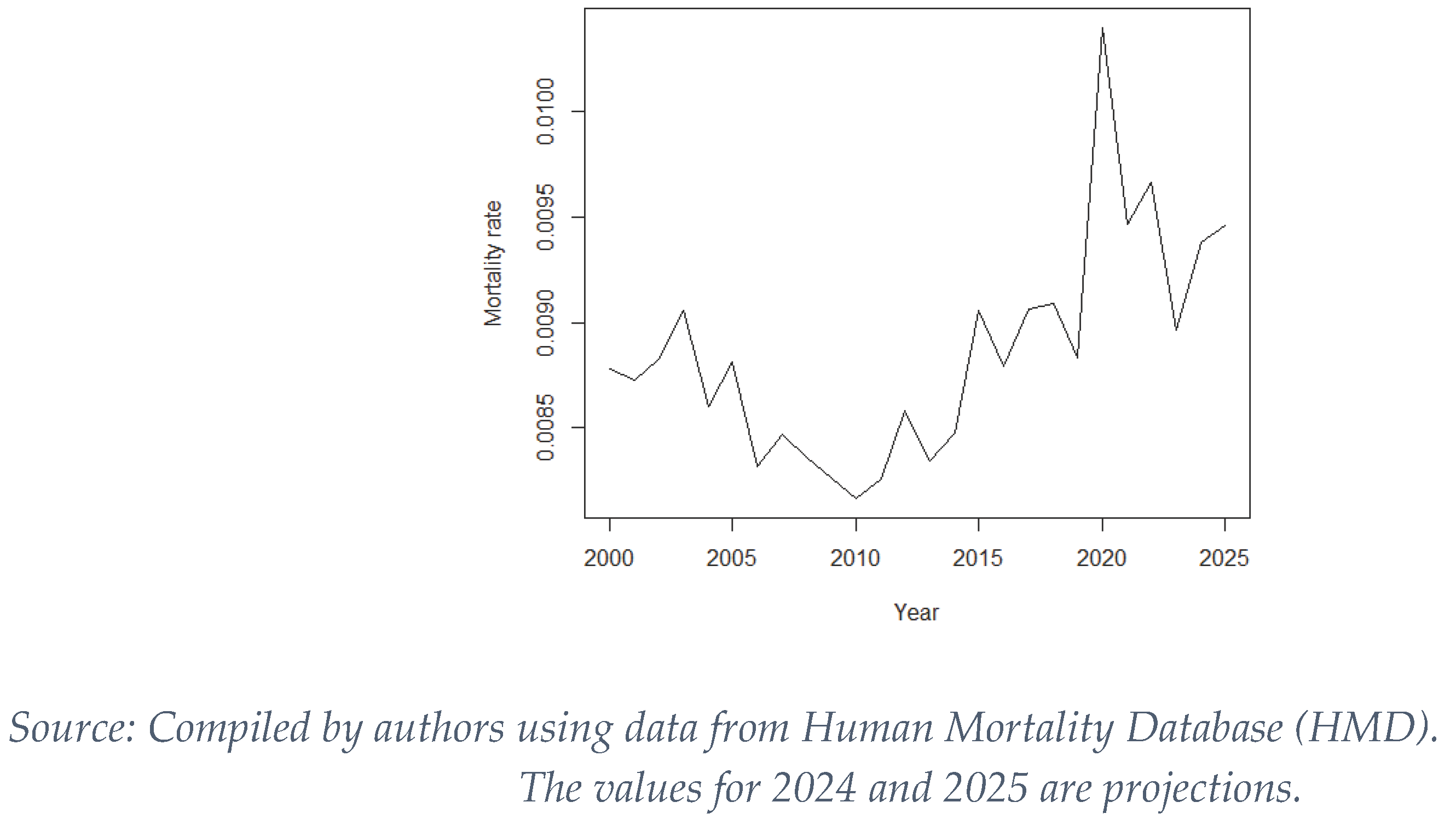
Figure 2.
Logarithmic mortality rates of Spain. Left panel: All ages. Right panel: Ages 20 to 60.
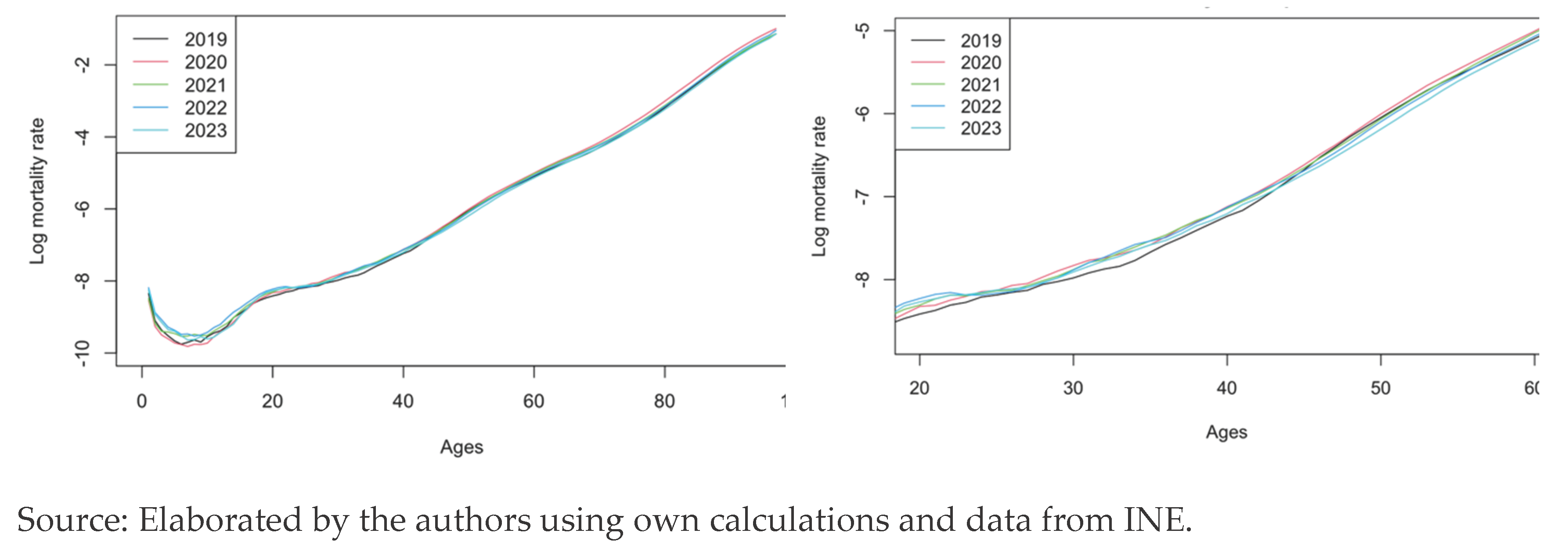
Figure 3.
Evolution of number of PEM – Lee-Carter model. Top left: Horizon of 1 year (2020). Top right: Horizon of 2 years (2021). Bottom left: Horizon of 3 years (2022). Bottom right: Horizon of 4 years (2023).
Figure 3.
Evolution of number of PEM – Lee-Carter model. Top left: Horizon of 1 year (2020). Top right: Horizon of 2 years (2021). Bottom left: Horizon of 3 years (2022). Bottom right: Horizon of 4 years (2023).
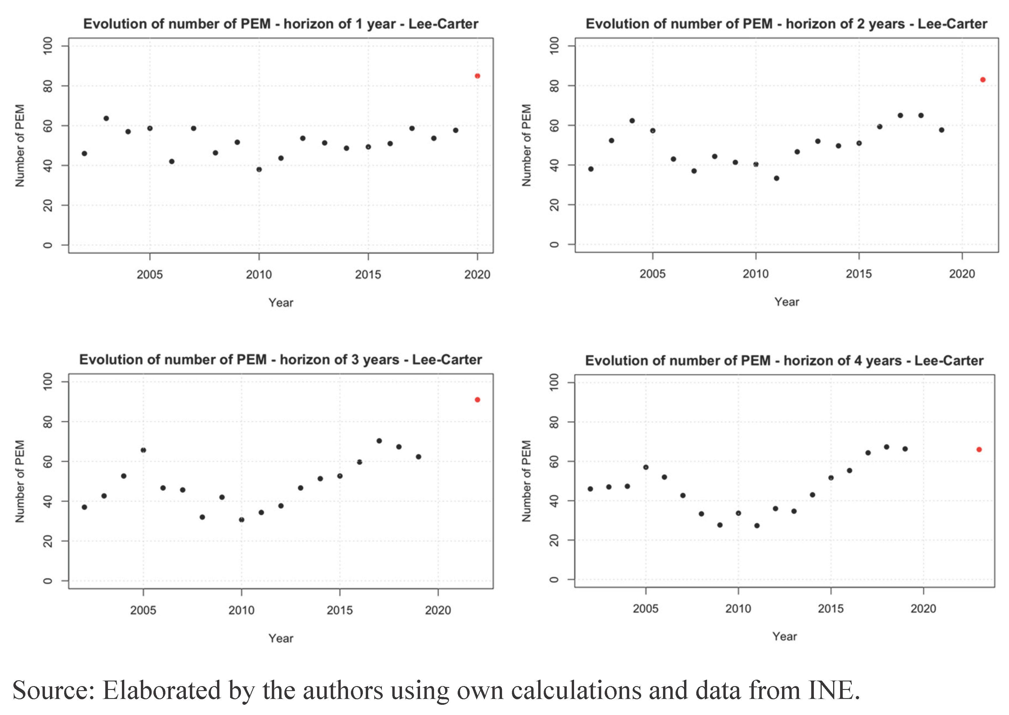
Figure 4.
Evolution of number of EM – Lee-Carter model. Top left: Horizon of 1 year (2020). Top right: Horizon of 2 years (2021). Bottom left: Horizon of 3 years (2022). Bottom right: Horizon of 4 years (2023).
Figure 4.
Evolution of number of EM – Lee-Carter model. Top left: Horizon of 1 year (2020). Top right: Horizon of 2 years (2021). Bottom left: Horizon of 3 years (2022). Bottom right: Horizon of 4 years (2023).
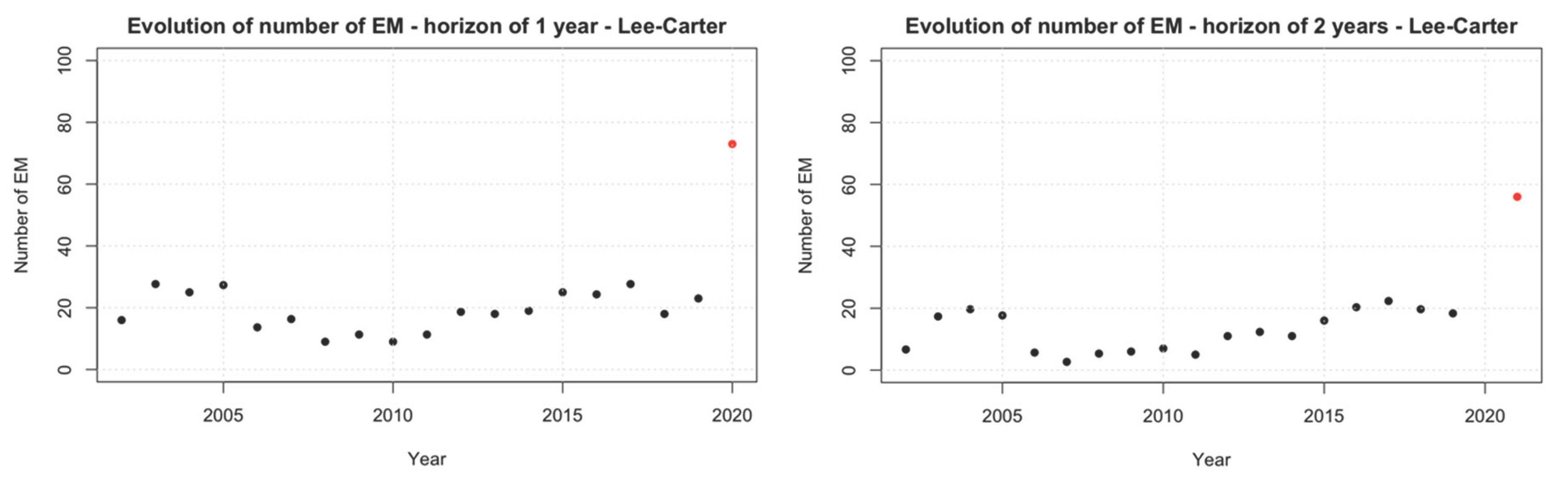
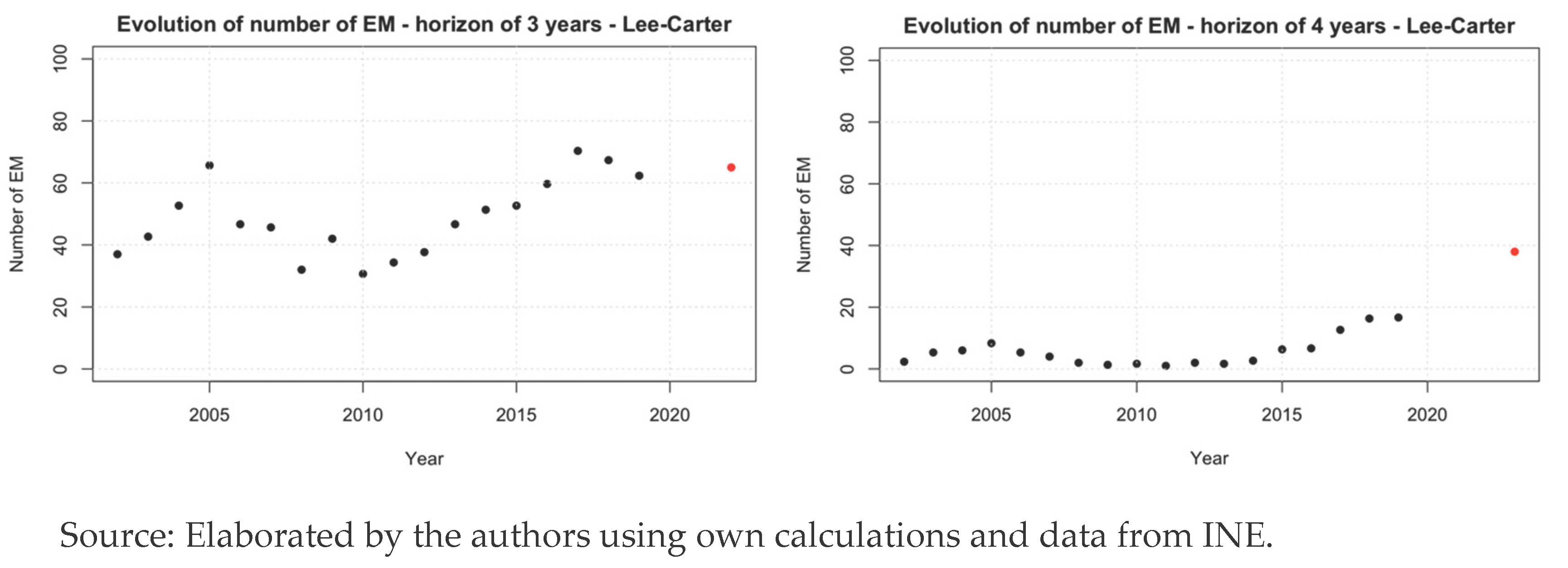
Figure 6.
Comparison of Excess of Mortality using a ratio.
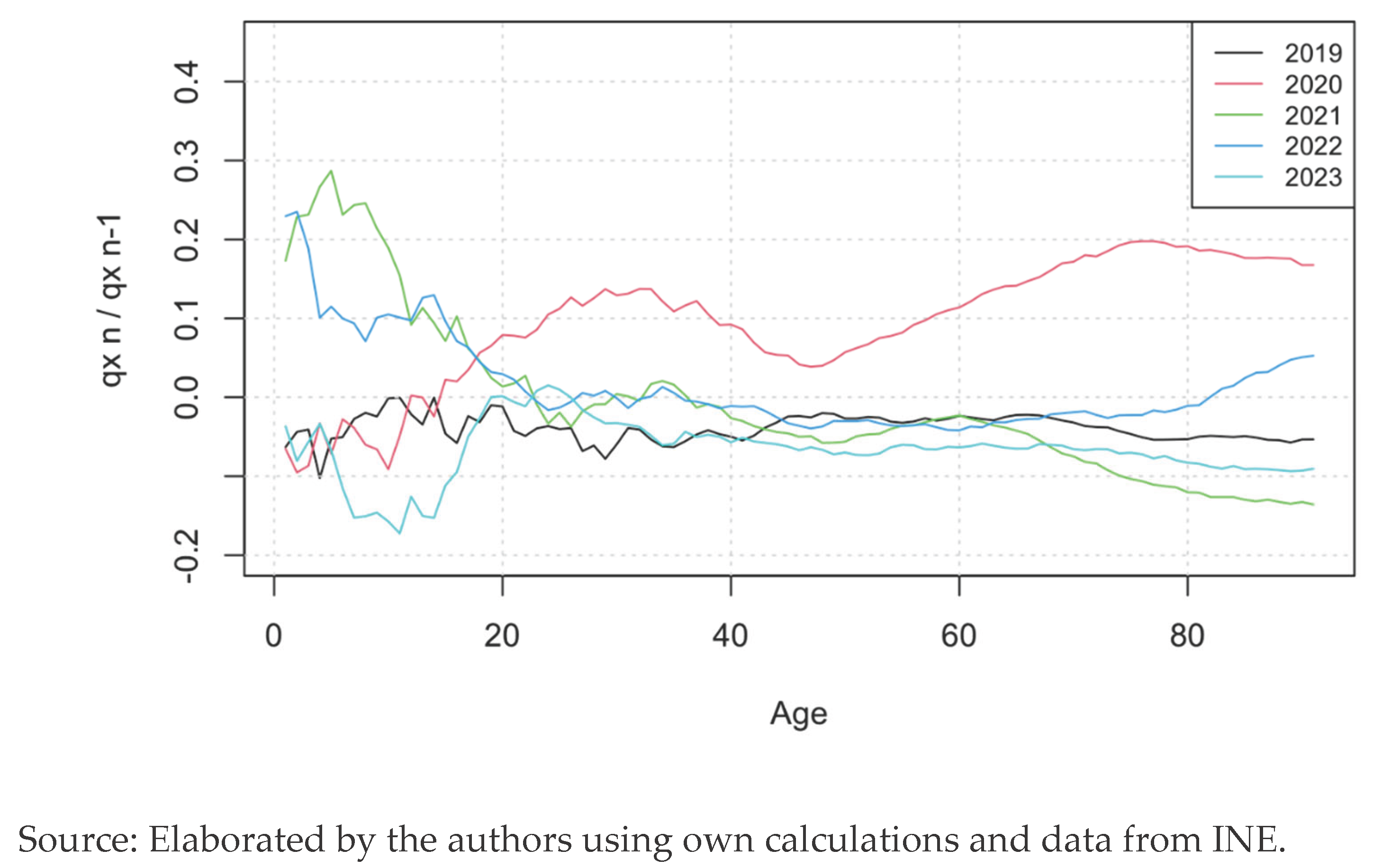
Table 1.
Akaike and Bayesian Information Criteria of the used models jointly with Deviance.
| Model | Lee-Carter | CBD | APC | Model | Lee-Carter | CBD | APC | |
| AIC | 39273 | 947111 | 35785 | AIC | 12497 | 18655 | 11758 | |
| BIC | 40656 | 947471 | 37300 | BIC | 12931 | 18944 | 12298 | |
| Deviance | 11822 | 919961 | 8290 | Deviance | 2431 | 8760 | 1648 | |
| Left panel: All ages. | Right panel: Ages 70 to 100 |
Source: Compiled by the authors. Data for years 2024 and 2025 are projections.
Table 3.
Number of ages with PEM in Lee – Carter model. (by decadal groups of age).
| Age | 2020 | 2021 | 2022 | 2023 | 2024* | 2025* |
|---|---|---|---|---|---|---|
| 1-10 | 8 | 9 | 10 | 10 | 9 | 9 |
| 11-20 | 4 | 10 | 10 | 7 | 10 | 10 |
| 21-30 | 10 | 10 | 10 | 10 | 10 | 10 |
| 31-40 | 10 | 10 | 10 | 10 | 10 | 10 |
| 41-50 | 4 | 4 | 5 | 5 | 10 | 10 |
| 51-60 | 8 | 6 | 6 | 2 | 10 | 10 |
| 61-70 | 10 | 10 | 10 | 10 | 10 | 10 |
| 71-80 | 10 | 10 | 10 | 10 | 10 | 10 |
| 81-90 | 10 | 10 | 10 | 2 | 10 | 10 |
| 91-100 | 10 | 4 | 10 | 0 | 10 | 10 |
| Total | 84 | 83 | 91 | 66 | 99 | 99 |
Source: Compiled by the authors. Data for years 2024 and 2025 are projections.
Table 4.
Number of ages which have an EM in Lee – Carter model.
| Age | 2020 | 2021 | 2022 | 2023 | 2024* | 2025* |
|---|---|---|---|---|---|---|
| 0-10 | 3 | 5 | 9 | 9 | 8 | 8 |
| 11-20 | 3 | 6 | 8 | 3 | 6 | 6 |
| 21-30 | 10 | 10 | 10 | 10 | 9 | 9 |
| 31-40 | 9 | 10 | 8 | 9 | 9 | 9 |
| 41-50 | 1 | 1 | 1 | 0 | 0 | 0 |
| 51-60 | 6 | 2 | 1 | 0 | 0 | 0 |
| 61-70 | 10 | 10 | 10 | 7 | 5 | 4 |
| 71-80 | 10 | 10 | 9 | 0 | 6 | 5 |
| 81-90 | 10 | 2 | 1 | 0 | 1 | 2 |
| 91-100 | 10 | 0 | 8 | 0 | 2 | 0 |
| Total | 73 | 56 | 65 | 38 | 46 | 43 |
Source: Compiled by the authors. Data for years 2024 and 2025 are projections.
Table 5.
REM by ages in Lee-Carter model.
| Age | 2020 | 2021 | 2022 | 2023 | 2024* | 2025* |
|---|---|---|---|---|---|---|
| 1-10 | 5,8% | 26,2% | 57,4% | 56,5% | 116.3% | 132.6% |
| 11-20 | 3% | 21,8% | 38,4% | 17,8% | 45.5% | 53.2% |
| 21-30 | 48,3% | 57,8% | 70,5% | 78,7% | 53.8% | 61.3% |
| 31-40 | 42,5% | 49,2% | 54,9% | 57,4% | 56.6% | 64.6% |
| 41-50 | 0,5% | 0,2% | 1,8% | -0,8% | 23.2% | 27.4% |
| 51-60 | 5,9% | 2,3% | 0,7% | -5,2% | 7.7% | 9.1% |
| 61-70 | 21% | 19,8% | 17,4% | 12,2% | 12.4% | 14% |
| 71-80 | 22,6% | 15,1% | 15,6% | 10,2% | 18.9% | 21.4% |
| 81-90 | 18,2% | 5,6% | 6,3% | -1% | 14% | 16.2% |
| 91-100 | 14,8% | 0% | 6,1% | -2,8% | 6.3% | 6.8% |
Source: Compiled by the authors. Data for years 2024 and 2025 are projections.
Disclaimer/Publisher’s Note: The statements, opinions and data contained in all publications are solely those of the individual author(s) and contributor(s) and not of MDPI and/or the editor(s). MDPI and/or the editor(s) disclaim responsibility for any injury to people or property resulting from any ideas, methods, instructions or products referred to in the content. |
© 2026 by the authors. Licensee MDPI, Basel, Switzerland. This article is an open access article distributed under the terms and conditions of the Creative Commons Attribution (CC BY) license (http://creativecommons.org/licenses/by/4.0/).
Copyright: This open access article is published under a Creative Commons CC BY 4.0 license, which permit the free download, distribution, and reuse, provided that the author and preprint are cited in any reuse.


