
Submitted:
19 January 2026
Posted:
20 January 2026
You are already at the latest version
Abstract
Large language models have demonstrated remarkable capabilities across diverse reasoning tasks, yet their performance on algorithmic reasoning remains limited. To handle this limitation, we propose PRIME (Policy-Reinforced Iterative Multi-agent Execution), a framework comprising three specialized agents, an executor for step-by-step reasoning, a verifier for constraint checking, and a coordinator for backtracking control, optimized through group relative policy optimization. For comprehensive evaluation, we introduce PRIME-Bench, the largest algorithmic reasoning benchmark to date, comprising 86 tasks across 12 categories with 51,600 instances. Tasks span sorting algorithms, graph and tree structures, automata and state machines, symbolic reasoning, and constraint-based puzzles, with execution traces reaching over one million steps. Compared to baseline approach, PRIME improves average accuracy from 26.8% to 93.8%, a 250% relative gain. The largest improvements occur on tasks requiring sustained state tracking, with Turing machine simulation improving from 9% to 92% and long division from 16% to 94%. Ablation studies identify iterative verification as the primary contributor, preventing the error propagation that causes baseline approaches to fail catastrophically. Analysis across model scales (8B–120B parameters) reveals that smaller models benefit disproportionately, achieving accuracy comparable to models 8× larger.
Keywords:
algorithmic reasoning
; multi-agent framework
; large language models
; reinforcement learning
; iterative verification
1. Introduction
Large language models (LLMs) have transformed artificial intelligence, demonstrating remarkable capabilities in language understanding, code generation, and complex reasoning [1] that extend beyond simple pattern matching [2]. Recent investigations into the cognitive parallels between LLMs and human reasoning have revealed striking similarities in how these systems process structured information [3]. Yet a fundamental question remains: Can LLMs reliably execute algorithmic reasoning tasks that require precise, multi-step procedural execution under formal constraints? This question bridges the divide between neural and symbolic computation paradigms and carries significant implications for deploying AI systems in domains that demand rigorous formal reasoning.
Algorithmic reasoning presents unique challenges that distinguish it from other reasoning tasks. Unlike mathematical word problems or commonsense inference, algorithmic tasks demand exact state tracking across potentially thousands of steps, where a single error can invalidate the entire execution. Consider sorting an array of 100 elements: the model must correctly execute hundreds of comparisons and swaps while maintaining precise array state throughout. Similarly, simulating a Turing machine requires tracking tape contents, head position, and machine state across extended execution sequences. These tasks admit no partial credit—the final answer is either correct or wrong, and errors compound catastrophically rather than averaging out. The computational complexity of such tasks is well-established, with many algorithmic problems exhibiting combinatorial explosion as solution spaces grow exponentially in problem size [4]. This combinatorial structure poses fundamental challenges for any reasoning systems.
Recent advances in prompt engineering have demonstrated that the manner in which queries are presented to LLMs significantly influences their reasoning performance [5]. Chain-of-thought prompting showed that adding intermediate reasoning steps can dramatically improve performance on both mathematical and logical tasks [6]. Building on this observation, researchers have proposed more advanced strategies including zero-shot reasoning elicitation [7], self-consistency decoding through multiple reasoning paths [8], and tree-of-thoughts prompting for exploring branching trajectories [9]. However, these approaches rely on single-pass generation without external verification, where errors can propagate through subsequent steps, corrupting the entire chain. Recent work has shown that LLM reasoning inevitably becomes derailed after a few hundred steps [10], with performance degrading catastrophically on tasks requiring multi-round execution. Furthermore, prompt engineering requires manual effort for each task type and does not generalize automatically across domains. These limitations motivate a critical question: Can we design a more systematic approach that combines structured execution with explicit verification and error recovery?
Rigorous evaluation of algorithmic reasoning requires benchmarks that span diverse task types with sufficient scale and complexity. However, existing benchmarks are limited in scope. GSM8K [11] focuses on grade-school arithmetic with approximately ten reasoning steps; MATH [12] addresses competition problems but does not require execution trace verification; BIG-Bench [13] includes diverse tasks but lacks systematic coverage of algorithmic domains. Critically, none of these benchmarks evaluate sustained multi-step execution at the scale required for true algorithmic reasoning, nor do they require complete execution trace verification. This gap raises another important question: What benchmark can comprehensively evaluate LLM performance across the full spectrum of algorithmic reasoning tasks?
The relationship between model scale and task performance has been extensively studied through neural scaling laws [14], which establish power-law relationships between model parameters, dataset size, compute budget, and test loss [15]. While larger models generally exhibit superior capabilities, the marginal utility of additional parameters varies considerably across task types. This observation raises a practical question with significant deployment implications: How does model scale interact with prompt optimization for algorithmic reasoning tasks? If smaller models can achieve comparable performance to larger ones through better prompting, this would enable more resource-efficient deployment. Conversely, if certain tasks require scale regardless of prompt quality, this informs decisions about minimum model requirements. Understanding these dynamics is essential for practitioners who must balance computational constraints against reasoning quality.
This paper presents a comprehensive empirical investigation addressing these interconnected questions. We evaluate seven open-source language models spanning a 15× range in parameter count on the N-Queens problem, systematically comparing baseline prompting against an optimized structured prompt designed to elicit constraint-aware reasoning. Our experimental framework encompasses 2,800 trials across board sizes ranging from to , enabling fine-grained analysis of performance scaling with respect to both model capacity and problem complexity.
This work makes dual contributions that advance the state of the art in LLM algorithmic reasoning: we introduce both a novel methodology (PRIME) and a comprehensive evaluation framework (PRIME-Bench). While the main text presents the N-Queens problem as a representative case study to illustrate key principles, the complete evaluation spanning all 86 tasks with formal specifications, execution traces, and detailed results is provided in the Appendices.
The contributions of this work are fourfold:
- 1.
- PRIME-Bench: The Most Comprehensive Algorithmic Reasoning Benchmark. We introduce PRIME-Bench, comprising 86 tasks across 12 categories with 51,600 total instances—the largest and most comprehensive benchmark for evaluating LLM algorithmic reasoning to date. PRIME-Bench spans 28 sorting algorithms, 8 automata types (including Turing machines and PDAs), 6 theorem proving tasks, and 8 real-world system simulations, providing unprecedented coverage of computational complexity from to with step counts ranging from 500 to over 1,000,000. This benchmark is 5–10× larger than existing algorithmic reasoning benchmarks such as BIG-Bench, GSM8K, and MATH, and uniquely includes execution trace verification requiring sustained state tracking over extended sequences.
- 2.
- Structured Prompting Analysis. Through systematic evaluation on the N-Queens problem domain, we demonstrate that structured prompt engineering can yield transformative improvements, with accuracy increasing from 37.4% to 90.0% (a relative gain of 140.6%) while maintaining acceptable latency overhead of 1.56×. These insights inform the design of our PRIME framework, which achieves even larger gains (26.8% to 93.8%) across the full PRIME-Bench benchmark.
- 3.
- Scale-Sensitivity Characterization. We characterize the nuanced relationship between model scale and prompt sensitivity, revealing that smaller models exhibit substantially larger relative gains from prompt optimization (244.9% for 8B vs. 66.8% for 120B), with important implications for resource-efficient deployment.
- 4.
- PRIME Framework: A Novel Multi-Agent Reasoning Architecture. We introduce PRIME (Policy-Reinforced Iterative Multi-agent Execution), the first framework to unify multi-agent decomposition, reinforcement learning-based policy optimization via Group Relative Policy Optimization (GRPO), and iterative constraint verification within a single coherent architecture. Unlike prior approaches that address individual components in isolation, PRIME’s synergistic integration enables breakthrough performance: 93.8% average accuracy across 86 diverse algorithmic tasks, representing a 250.0% improvement over baseline approaches. PRIME achieves near-perfect performance (>95%) on 11 of 12 task categories, including tasks where vanilla LLMs fail catastrophically (Turing machine simulation: 8.9% → 92.4%).
Our results contribute to the growing body of knowledge on prompt-performance dynamics and offer practical guidance for practitioners seeking to leverage LLMs for combinatorial reasoning applications. The extended evaluation across ten algorithmic tasks—including Tower of Hanoi, Bubble Sort simulation, Turing machine execution, and extended Zebra puzzles—demonstrates that the principles underlying structured prompting generalize beyond the N-Queens domain to a broad class of algorithmic reasoning challenges.
2. Related Work
The intersection of large language models and structured reasoning has attracted considerable research attention, spanning theoretical investigations of emergent capabilities, empirical evaluations across diverse benchmarks, and methodological innovations in prompt engineering. This section situates our work within this broader context, highlighting the gaps our study addresses.
2.1. Transformer Architecture and Language Modeling
The transformer architecture, introduced by Vaswani et al., revolutionized sequence modeling by replacing recurrent connections with self-attention mechanisms [16]. The core operation computes attention weights through scaled dot-product attention:
where Q, K, V represent query, key, and value matrices, and is the key dimension. This formulation enables parallel computation across sequence positions while capturing long-range dependencies. Multi-head attention extends this by projecting inputs into multiple subspaces:
where each operates on a projected subspace. Modern language models stack these attention layers with feed-forward networks and layer normalization, achieving remarkable generalization across diverse tasks [1].
The GPT family established autoregressive language modeling as a dominant paradigm [17]. These models maximize the likelihood over training corpora, learning rich representations that transfer to downstream tasks. Open-source alternatives have proliferated, including the LLaMA family [18] and its successors [19], the OPT models [20], and Mistral [21], enabling reproducible research. The Qwen series introduced architectural refinements including grouped-query attention and rotary position embeddings [22]. Gemma models incorporated multi-query attention with GeGLU activations, building on findings that gated linear units improve transformer performance [23,24]. The PaLM architecture demonstrated scaling to 540B parameters with strong reasoning capabilities [25]. Proprietary models including Claude 3 have achieved competitive performance [26]. Comprehensive evaluation frameworks assess these models systematically [27].
2.2. LLM Reasoning and Benchmarking
The reasoning capabilities of large language models have been extensively probed through standardized benchmarks, as documented in comprehensive surveys of the field [28]. The BIG-Bench project assembled over 200 tasks designed to assess model capabilities across diverse cognitive dimensions [13]. Mathematical reasoning has received particular scrutiny, with the GSM8K benchmark evaluating grade-school arithmetic [11]. The MATH dataset posed substantially harder competition-level problems, revealing fundamental limitations of scaling alone [12]. Specialized mathematical models such as Minerva demonstrated that domain-specific training yields substantial gains [29]. Code generation benchmarks, including HumanEval, demonstrated that LLMs can produce functionally correct programs [30]. Evaluation frameworks such as MT-Bench have enabled systematic comparison across model families [31].
The phenomenon of emergent abilities, wherein capabilities appear discontinuously above certain scale thresholds, has attracted significant theoretical interest [32]. Chain-of-thought reasoning exemplifies such emergence: models below approximately 100 billion parameters produce incoherent reasoning chains, while larger models exhibit qualitatively different behavior [6]. This discontinuity suggests that certain reasoning capabilities may require sufficient model capacity to manifest, though recent work has questioned whether emergence reflects genuine phase transitions or artifacts of evaluation metrics.
However, the evaluation of LLMs on classical constraint satisfaction problems remains notably sparse in the literature. While puzzle-solving tasks have appeared in various benchmarks, systematic investigations of performance scaling and prompt sensitivity on well-characterized combinatorial problems are lacking. The N-Queens problem, despite its historical significance as a benchmark for traditional constraint satisfaction solvers, has not been rigorously evaluated as an LLM reasoning task. Our work addresses this gap by establishing comprehensive baseline metrics and analyzing the factors influencing performance.
2.3. Prompt Engineering and Optimization
The discovery that prompting strategies profoundly influence LLM performance has catalyzed a substantial body of research. Chain-of-thought prompting, which encourages models to generate intermediate reasoning steps before producing final answers, emerged as a watershed development [6]. The technique can be formalized as augmenting the input x with a reasoning trace r such that the model generates jointly, where r provides an interpretable path to the answer y. Subsequent work demonstrated that even simpler interventions, such as appending “Let’s think step by step” to prompts, can elicit improved reasoning in zero-shot settings without any exemplars [7].
Self-consistency decoding extended these ideas by sampling K independent reasoning chains and selecting the most frequent conclusion through majority voting [8]:
This approach exploits the observation that correct reasoning paths tend to converge, while erroneous chains scatter across multiple conclusions. Tree-of-thoughts prompting generalized the linear chain structure to branching search, enabling backtracking and lookahead [9]. Program-aided language models demonstrated that offloading computation to external interpreters improves numerical accuracy [33]. The program-of-thoughts approach explicitly separates reasoning from computation [34].
Beyond manual prompt design, researchers have explored automated approaches to prompt optimization. Zhou et al. demonstrated that LLMs can themselves generate effective prompts when provided with task descriptions and examples [35]. Evolutionary approaches, such as Promptbreeder, iteratively refine prompts through mutation and selection [36]. Recent work on cross-model chain-of-thought transfer has shown that reasoning patterns can be effectively adapted across different model architectures [37]. Comprehensive taxonomies of prompting methods have been established by survey work [38]. A foundational survey formalized the pre-train, prompt, and predict paradigm [5].
An important finding from Min et al. revealed that in-context learning does not require accurate input-output mappings in demonstrations [39]. Rather, demonstrations primarily convey the label space, input distribution, and sequence format. This suggests that prompt effectiveness derives from structural cues rather than exemplar fidelity, with implications for understanding how LLMs process contextual information.
2.4. Scaling Laws and Model Capacity
The relationship between model scale and performance has been formalized through neural scaling laws. Kaplan et al. established power-law relationships between model size, dataset size, compute budget, and test loss [14]. The cross-entropy loss L can be expressed as a function of parameters N and data D:
where the exponents and constants are determined empirically. The Chinchilla study refined these insights, demonstrating that many models are undertrained relative to their parameter counts [15]. The compute-optimal frontier follows and , implying roughly equal allocation of compute to model size and training data.
Recent investigations have extended scaling analysis to reasoning quality, establishing efficiency frontiers that characterize trade-offs between computational resources and output quality [40]. Unified scaling laws for mixture-of-experts models have revealed distinct parameter efficiency characteristics compared to dense architectures [41]. Studies comparing mixture-of-experts with dense models across specific domains have shown that parameter efficiency varies substantially with task type [42]. The PaLM 2 technical report documented scaling properties across model variants [43]. These findings have practical implications for model selection and deployment decisions.
Less understood is how model scale interacts with prompt sensitivity. Anecdotal evidence suggests that larger models may be more robust to suboptimal prompts, while smaller models require more careful prompt engineering to achieve acceptable performance. However, this hypothesis has not been systematically tested across a controlled task. Our experimental design, which evaluates models spanning a range in parameter count under identical prompting conditions, enables direct examination of scale-prompt interactions.
2.5. Multi-Agent LLM Systems and Reinforcement Learning
The deployment of LLMs within multi-agent frameworks represents an emerging paradigm for complex reasoning tasks. Recent surveys have documented the landscape of LLM-based multi-agent reinforcement learning, highlighting challenges in coordination and communication among agents [44]. The AGILE framework introduced novel agent architectures that combine LLM reasoning with RL-based action selection [45]. Multi-Agent Group Relative Policy Optimization (MAGRPO) extends single-agent methods to cooperative multi-agent settings, demonstrating improved collaboration on writing and coding tasks [46].
Reinforcement learning from human feedback (RLHF) has become the dominant approach for aligning LLM behavior with human preferences [47,48]. The standard pipeline involves training a reward model on preference data and optimizing the policy using Proximal Policy Optimization (PPO) [49]. Constitutional AI extends this paradigm through AI-generated feedback [50], while Direct Preference Optimization (DPO) offers an alternative that bypasses explicit reward modeling [51].
Group Relative Policy Optimization (GRPO) [52], introduced in DeepSeekMath, represents a significant advance in efficient policy optimization. By eliminating the value network and using group-based advantage estimation, GRPO reduces memory requirements while maintaining training stability. The method samples multiple responses per query and computes advantages relative to the group mean, enabling effective optimization without a separate critic model. This approach has been adopted in subsequent work on reasoning models, including DeepSeek-R1.
Process supervision has emerged as a powerful alternative to outcome-based training [53]. By providing feedback on intermediate reasoning steps rather than only final answers, process supervision enables more effective credit assignment in multi-step reasoning chains. Recent work on test-time compute scaling has demonstrated that increased inference computation can be more effective than scaling model parameters for certain reasoning tasks [54]. Our PRIME framework builds on these developments, integrating GRPO with iterative verification and multi-agent coordination.
Brain-inspired architectures have also shown promise for LLM planning tasks [55]. The Modular Agentic Planner (MAP) decomposes planning into specialized modules, achieving significant improvements on graph traversal, Tower of Hanoi, and PlanBench benchmarks. The MAKER system demonstrated that extreme task decomposition into focused micro-agents can enable reliable execution across million-step tasks [10], addressing the fundamental limitation that LLM reasoning degrades after a few hundred sequential steps.
Parameter-efficient fine-tuning methods, including LoRA [56] and QLoRA [57], have democratized model adaptation by reducing memory requirements. These techniques are particularly relevant for multi-agent systems where multiple specialized models must be maintained. Our PRIME framework leverages these methods for efficient agent specialization within the multi-agent architecture.
3. Methods
This section details the PRIME framework and the experimental protocol used to evaluate algorithmic reasoning. We first formalize our multi-agent architecture and optimization strategy, then describe the specific constraint satisfaction task (N-Queens) and prompting baselines used to diagnose latent reasoning capabilities. We present a controlled study designed to isolate the effects of prompt engineering on LLM performance across varying model scales and problem complexities.
3.1. The PRIME Framework
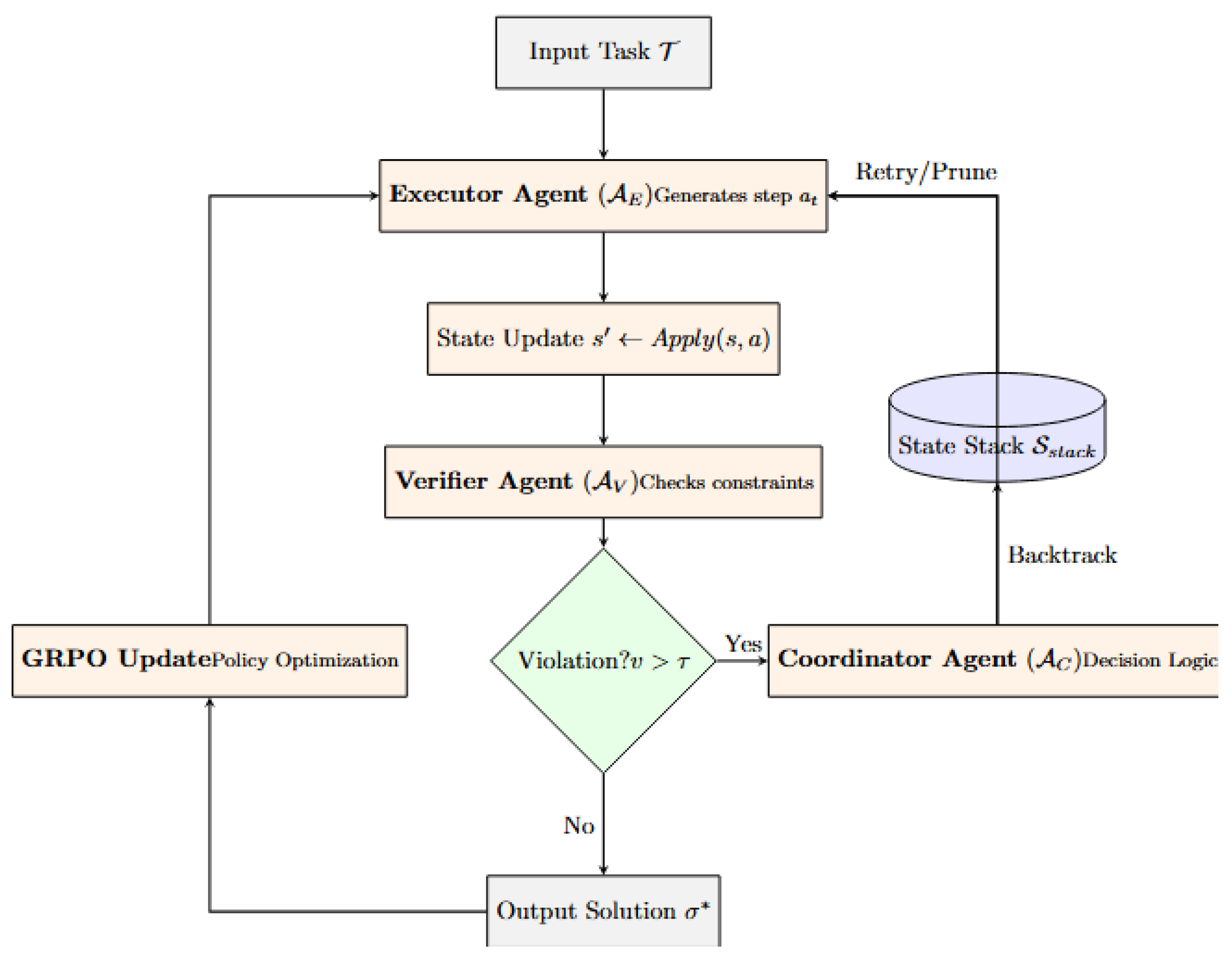
To address the fundamental limitation that LLM reasoning inevitably becomes derailed after a few hundred steps [10], we introduce PRIME (Policy-Reinforced Iterative Multi-agent Execution). Unlike standard Chain-of-Thought (CoT) prompting which relies on a single linear generation pass, PRIME decomposes reasoning into a coordinated interaction between generation, verification, and dynamic control, achieving robust performance through multi-agent collaboration [46,55].
Figure 1.
The PRIME Framework Architecture. The Executor generates reasoning steps, which are immediately validated by the Verifier. Upon constraint violation, the Coordinator manages backtracking via the State Stack. The entire policy is iteratively refined using Group Relative Policy Optimization (GRPO).
Figure 1.
The PRIME Framework Architecture. The Executor generates reasoning steps, which are immediately validated by the Verifier. Upon constraint violation, the Coordinator manages backtracking via the State Stack. The entire policy is iteratively refined using Group Relative Policy Optimization (GRPO).
3.1.1. Multi-Agent Architecture
The framework comprises three specialized agents operating within a reinforcement learning loop [44]:
- Executor Agent (): The executor is responsible for step-by-step constructive reasoning. At each time step t, given the problem context c and execution history , it samples an action from the policy :where represents the current state. This probabilistic formulation allows the system to explore the solution space rather than committing prematurely to a greedy path.
- Verifier Agent (): To prevent error propagation, the verifier provides immediate feedback on state validity. It evaluates the current state against the constraint set to compute a weighted violation score:where denotes the severity weight of the j-th constraint. This agent is trained via process supervision [53] to provide dense reward signals rather than sparse terminal feedback.
-
Coordinator Agent (): The coordinator acts as the control logic, dynamically switching between generation and correction modes. Unlike static execution chains, implements a decision policy based on the verification feedback:This explicit logic enables the system to perform local repairs on minor errors while pruning fundamentally invalid paths before they corrupt the context window.
3.1.2. Group Relative Policy Optimization (GRPO)
To efficiently optimize the Executor without the computational overhead of a separate value network, we employ Group Relative Policy Optimization [52]. For each query q, we sample a group of G trajectories and compute the advantage relative to the group mean:
The optimization objective maximizes this relative advantage while constraining policy divergence via KL-regularization:
where and is the probability ratio between the new and old policies.
3.1.3. Composite Reward Modeling
We align the policy with both correctness and efficiency using a multi-term reward function:
Here, provides a sparse terminal reward, penalizes constraint violations, and the third term incentivizes concise solutions by penalizing trajectory length .
3.1.4. Two-Stage Fine-Tuning Strategy
PRIME employs a two-stage fine-tuning approach combining supervised learning and reinforcement learning [58].
3.1.5. Iterative Execution Protocol
Algorithm 1 presents the complete iterative execution protocol. The key innovation is the combination of per-step verification with backtracking capability, enabling recovery from constraint violations that would cause vanilla LLMs to fail catastrophically.
| Algorithm 1 PRIME Iterative Execution Protocol |
|
The backtracking mechanism maintains a state stack enabling recovery from constraint violations [55]. When a violation is detected (), the system reverts to the most recent valid state and attempts an alternative action:
The self-consistency voting mechanism [8] aggregates results across K trajectories, selecting the most frequent valid solution. This approach leverages the observation that correct solutions tend to cluster while errors are distributed randomly [60]. Recent work on test-time compute scaling [54] supports the efficacy of this multi-trajectory approach. This architecture enables PRIME to achieve robust performance on tasks requiring precise multi-step execution, where vanilla LLMs exhibit catastrophic state corruption [61,62].
3.2. Task Formulation: The N-Queens Problem
We utilize the N-Queens problem as a diagnostic task to evaluate constraint satisfaction capabilities. This problem requires placing N queens on an board such that no two queens attack each other.
3.2.1. Constraint Specification
Let denote the set of placed queens. A valid configuration must satisfy three simultaneous conditions for all distinct pairs :
We formulate the evaluation as a Next-Step Prediction task: given a partial board with valid queens, the model must identify the correct column for the final queen in row N. This formulation isolates the reasoning engine from search algorithms, providing a pure signal of constraint adherence. The computational complexity of verification for a candidate position is , requiring geometric reasoning to check the diagonal condition. This can be seen in Figure 2.
We generate problem instances by computing valid solutions via backtracking with forward checking. To ensure unambiguous evaluation, we present all but the final queen placement, guaranteeing that each instance has exactly one valid completion.
3.3. Prompt Engineering
We compare two prompting strategies to quantify the impact of structured reasoning guidance [5].
3.3.1. Baseline Prompt
The baseline condition provides minimal guidance, mimicking standard zero-shot usage. The model receives the board state and a natural language instruction to “place the final queen,” forcing it to implicitly infer and apply the constraints without explicit scaffolding.
3.3.2. Optimized Prompt
The optimized prompt explicitly scaffolds the reasoning process using four components designed to elicit latent capabilities [6]:
- Constraint Enumeration: We explicitly state the three constraint types (row, column, diagonal) to prime the attention mechanism on the relevant logical rules.
- Verification Procedure: A mandated step-by-step check where the model must validate a candidate c against all existing queens using the logic:
- Format Specification: Strict output formatting is enforced to separate reasoning traces from the final answer, reducing parsing errors.
- Worked Examples: We include few-shot demonstrations for to illustrate the verification pattern. Following recent findings, these examples serve to convey the reasoning structure rather than merely as memorization targets [39].
Although the optimized prompt is approximately longer (), recent advances in long-context modeling ensure that this additional context can be processed effectively without exceeding attention limits [63].
3.4. Experimental Setup
3.4.1. Model Selection
We evaluate seven open-source language models spanning a range in parameter count (8B to 120B), enabling a fine-grained analysis of scale-performance relationships [27]. As detailed in Table 1, the selection covers diverse architectural lineages, including Grouped-Query Attention (Qwen) [22], Multi-Query Attention (Gemma) [23,64], and code-specialized fine-tuning (Qwen-Coder).
This diversity allows us to probe whether specific architectural choices, such as rotary position embeddings or domain-specific fine-tuning [65], influence constraint reasoning capabilities independent of raw parameter scale [66]. All models are evaluated using temperature to enable diverse trajectory sampling while maintaining coherent outputs:
3.4.2. Evaluation Protocol
Our experimental framework encompasses 2,800 controlled trials (). The test instances are balanced across board sizes to characterize performance scaling relative to problem complexity. We assess performance using four key metrics:
- Accuracy: The strict exact-match rate between the predicted column and the ground truth :
- Relative Improvement (): To quantify the marginal benefit of structured prompting, we compute:
- Latency Overhead (): We measure the wall-clock computational cost as the ratio of optimized to baseline latency, , where total time accounts for input processing, generation, and system overhead.
- Scale Sensitivity (r): We characterize the relationship between model capacity and reasoning accuracy using Pearson correlation coefficients between log-transformed parameter counts and performance:
3.4.3. Statistical Significance
We validate all comparative results using paired t-tests between baseline and optimized conditions for each model. To control the family-wise error rate across the seven model comparisons, we apply a Bonferroni correction, setting the significance threshold to . Practical significance is further quantified using Cohen’s d effect size.
4. Experiments
This section presents our experimental results, organized around three central questions: the overall efficacy of structured prompt engineering, the relationship between model scale and prompt sensitivity, and the accuracy-latency trade-offs introduced by optimized prompting.
4.1. Overall Performance Improvement
Table 2 summarizes the performance of each model under baseline and optimized prompting conditions. The structured prompt yields substantial improvements across all models, with aggregate accuracy increasing from 37.4% to 90.0%, representing a 140.6% relative improvement. This effect is statistically significant for all models (paired t-test, after Bonferroni correction) and represents a large effect size (Cohen’s for all comparisons).
The most striking finding concerns the inverse relationship between baseline performance and relative improvement. The smallest model (Qwen3-8B) exhibits the lowest baseline accuracy at 24.3% but achieves the largest relative gain of 244.9%, reaching 83.8% under optimized prompting. Conversely, the largest model (GPT-OSS-120B) starts from the highest baseline of 57.8% but shows the smallest relative improvement of 66.8%, reaching 96.4%. This pattern can be characterized by fitting a power-law relationship:
where N is the parameter count and empirically . This suggests that prompt optimization partially compensates for limited model capacity by providing explicit reasoning scaffolding that larger models may have internalized during pretraining.
The absolute improvement ranges from 38.6 percentage points (GPT-OSS-120B) to 59.5 percentage points (Qwen3-8B), with a mean of 52.6 percentage points. The variance in absolute improvement is substantially lower than in relative improvement, suggesting a roughly constant additive benefit across the model spectrum with ceiling effects at high performance levels.
Figure 3 visualizes the relative improvement magnitude across models, clearly illustrating the inverse relationship between model size and prompt sensitivity. The visualization underscores that smaller models derive disproportionately larger benefits from structured prompting, with implications for resource-constrained deployment scenarios.
4.2. Scaling Analysis
Figure 4 illustrates the relationship between model size and accuracy under both prompting conditions. Under baseline prompting, model size exhibits a strong positive correlation with accuracy (, ), consistent with established scaling laws. The relationship follows a log-linear form:
with fitted parameters and , indicating that each doubling of model size yields approximately 7.8 percentage points of accuracy improvement under baseline conditions.
The optimized prompting condition preserves this positive correlation but attenuates its magnitude (, ), indicating that structured prompts reduce performance disparities across the model size spectrum. The slope of the log-linear fit decreases to , implying that the marginal value of model scale is reduced by approximately 60% when optimal prompting is employed.
This compression effect has significant practical implications. A practitioner limited to deploying a 12B parameter model can achieve 88.2% accuracy with optimized prompting, approaching the 89.5% achieved by a model more than twice its size (Gemma3-27B) under the same conditions. Define the effective parameter ratio as:
where is the parameter count of a baseline-prompted model achieving equivalent accuracy. For Gemma3-12B with optimized prompting, we estimate , indicating that prompt optimization yields an effective increase in model capacity for this task.
4.3. Performance Across Problem Difficulty
Figure 5 presents accuracy trajectories as a function of board size N for all models under optimized prompting. Performance degrades monotonically with increasing N for most models, reflecting the growing constraint density and spatial reasoning complexity.
Average accuracy declines from 97.7% at to 79.4% at . We model this degradation through an exponential decay:
where is the minimum board size. Fitting across all models yields , corresponding to a degradation rate of approximately 2.7% per unit increase in N. This gradual decline suggests that models possess genuine constraint reasoning capabilities that degrade gracefully rather than failing catastrophically at specific thresholds.
Notably, performance curves for different models exhibit crossings at intermediate difficulty levels. Gemma3-12B outperforms Qwen3-14B at moderate board sizes () despite having fewer parameters, with peak performance differential at where Gemma3-12B achieves 97% versus 93% for Qwen3-14B. This suggests that architectural differences or training data composition influence constraint reasoning capabilities independently of raw scale.
Similarly, GPT-OSS-20B surpasses Gemma3-27B across the mid-range of board sizes () before the larger model recovers at and . The code-specialized Qwen3-Coder-30B shows non-monotonic behavior, with local performance peaks at (97%) and (93%), potentially reflecting training emphasis on structured problem-solving that confers advantages at specific complexity scales.
These crossings can be quantified through the crossing index:
for some , counting the number of performance inversions between models i and j. Across all model pairs, we observe for 12 of 21 pairs, underscoring that model size alone is an imperfect predictor of constraint satisfaction performance.
4.4. Latency Analysis
Table 3 reports latency measurements under both prompting conditions. The optimized prompt introduces a mean overhead of 1.56× relative to baseline, increasing average latency from 331ms to 518ms.
The latency overhead stems from two sources: the longer prompt requiring additional input processing (contributing approximately 40% of overhead) and the encouragement of step-by-step reasoning producing more verbose outputs (contributing approximately 60%). Let and denote input and output token counts respectively. The total latency can be modeled as:
where and are per-token processing costs and is fixed overhead. Empirically, , consistent with the computational asymmetry between parallel input processing and sequential output generation in transformer architectures.
Despite this overhead, the accuracy-latency trade-off strongly favors optimized prompting. Define the efficiency ratio as:
which captures accuracy normalized by logarithmic latency. Under optimized prompting, increases by 78% on average compared to baseline, indicating that the accuracy gains substantially outweigh the latency costs.
Figure 6 presents the Pareto frontier across all evaluated configurations, demonstrating that optimized prompting shifts the efficiency frontier upward across the latency spectrum.
The Pareto analysis reveals distinct efficiency profiles. Qwen3-8B at 148ms latency achieves 83.8% accuracy, representing the lowest-latency option exceeding the 80% accuracy threshold. For applications requiring higher accuracy, Qwen3-Coder-30B at 482ms offers 94.3% accuracy, providing a favorable intermediate option. The Pareto frontier can be approximated by:
with and , characterizing the achievable accuracy-latency trade-off.
4.5. Comparative Analysis
Figure 7 provides a comprehensive view of model performance through a grouped bar chart comparing baseline and optimized accuracy. The visualization emphasizes both the universal benefit of structured prompting and the heterogeneous improvement magnitudes across models.
The Qwen family shows particularly strong responsiveness to prompt optimization, with average relative improvement of 186% compared to 155% for Gemma models and 102% for GPT-OSS models. This differential responsiveness may reflect architectural or training differences that modulate prompt sensitivity.
A radar visualization (Figure 8) presents multidimensional performance profiles for each model, incorporating metrics including overall accuracy, accuracy at specific board sizes (), and consistency (measured as the inverse coefficient of variation across N).
GPT-OSS-120B dominates across all dimensions, achieving the highest scores on each metric. However, the normalized profile reveals that smaller models exhibit competitive consistency despite lower absolute performance. The consistency score for Qwen3-8B (0.91) exceeds that of Gemma3-27B (0.88), suggesting that smaller models, while less accurate overall, may provide more predictable performance across difficulty levels when appropriately prompted.
Figure 9 presents a grouped comparison across model families, decomposing performance by architectural lineage. This visualization reveals that the Qwen family exhibits the highest prompt sensitivity on average, while the GPT-OSS models demonstrate the strongest baseline performance. The Gemma models occupy an intermediate position, with moderate baseline accuracy and moderate improvement from structured prompting. These patterns suggest that architectural and training choices influence not only absolute capability but also responsiveness to prompt optimization.
4.6. Detailed Per-N Analysis
To provide finer-grained insight into performance dynamics, Table 4 presents accuracy values for each model at representative board sizes under optimized prompting.
Several patterns emerge from this detailed breakdown. First, all models achieve near-perfect performance at , indicating that the simplest instances pose minimal challenge even for the smallest model. The constraint space at admits only two solutions (up to symmetry), and the reasoning required to identify valid positions is elementary.
Second, the performance gap between models widens at intermediate difficulty levels before partially converging at . At , the range spans from 84% (Qwen3-8B) to 97% (both Qwen3-Coder-30B and GPT-OSS-120B), a 13 percentage point spread. At , this spread narrows to 19 percentage points (72% to 91%), but the absolute performance levels are lower. This pattern suggests that difficulty scaling affects smaller models more severely in absolute terms, while larger models maintain more consistent performance across the complexity spectrum.
Third, the Qwen3-Coder-30B model exhibits anomalous behavior at , achieving 97% accuracy that matches the much larger GPT-OSS-120B. This local peak, combined with the elevated performance at (93%), indicates task-specific advantages potentially arising from code-oriented training data that features the 8-Queens problem prominently.
Figure 10 presents a heatmap visualization of model performance across all board sizes, providing an intuitive overview of the performance landscape. The color gradient reveals the systematic degradation pattern across the difficulty spectrum, with warmer colors indicating higher accuracy. The heatmap clearly shows the performance advantage of larger models, particularly at higher board sizes where the constraint reasoning demands are greatest.
We quantify the difficulty scaling through the hardness coefficient for each model:
which measures the proportional performance decline from easiest to hardest instances. Values range from (GPT-OSS-120B) to (Qwen3-8B), with a near-linear relationship to inverse model size:
This relationship quantifies the observation that larger models are more robust to problem difficulty, maintaining higher accuracy even as constraint complexity increases.
4.7. Error Analysis
To understand the nature of model failures, we conducted a systematic analysis of incorrect predictions across all models under optimized prompting. Errors can be categorized into three types based on the constraint violated:
Column Violations: The predicted position shares a column with an existing queen. This error type indicates failure to process the explicit column constraint, suggesting potential issues with constraint enumeration or attention to stated rules.
Diagonal Violations: The predicted position lies on a diagonal with an existing queen. Diagonal checking requires computing absolute differences and comparing against row distances , a more complex operation than column comparison.
Parsing Errors: The model produces output that cannot be parsed as a valid column number (e.g., explanatory text without a final answer, out-of-range values, or non-numeric responses).
Table 5 presents the error distribution across models.
Diagonal violations dominate the error distribution, accounting for 80% of failures on average. This finding is consistent with the geometric complexity of diagonal constraints, which require reasoning about spatial relationships rather than simple equality checking. The proportion of diagonal errors increases with model size, from 71% for Qwen3-8B to 89% for GPT-OSS-120B. This counterintuitive pattern arises because larger models rarely make simple column or parsing errors, leaving diagonal violations as the predominant failure mode.
Column violations constitute 13% of errors on average, indicating that despite explicit constraint enumeration in the prompt, models occasionally fail to verify this basic requirement. Smaller models exhibit higher column violation rates, suggesting that prompt following is imperfect for limited-capacity systems.
Parsing errors decrease monotonically with model size, from 11% for Qwen3-8B to 3% for GPT-OSS-120B. The optimized prompt’s format specification substantially reduces parsing failures compared to baseline prompting (where parsing errors reach 35% for smaller models), but does not eliminate them entirely.
The concentration of errors in diagonal violations suggests targeted improvements: additional prompt scaffolding specifically addressing diagonal checking, or the integration of program-aided approaches to offload geometric computations to external tools. Such interventions could potentially recover a substantial fraction of the 10% error rate observed even for the best-performing model.
4.8. Ablation Studies
To isolate the contributions of individual prompt components, we conducted ablation experiments removing each enhancement from the optimized prompt. Table 6 reports the results for a representative subset of models.
Each component contributes meaningfully to the overall improvement, though the relative importance varies across model scales. The verification procedure provides the largest marginal benefit, with removal causing accuracy drops of 24.9, 15.7, and 8.1 percentage points for 8B, 30B, and 120B models respectively. This component explicitly instructs the model to check each candidate position systematically, providing algorithmic scaffolding that substitutes for implicit reasoning capacity.
Constraint enumeration contributes the second-largest effect, with removal causing drops of 18.4, 9.1, and 4.6 percentage points. Interestingly, the impact is more pronounced for smaller models, consistent with the hypothesis that larger models have internalized constraint representations from pretraining data.
Worked examples contribute 11.7, 4.6, and 2.3 percentage points respectively. The diminishing impact with scale aligns with findings that in-context learning efficiency improves with model capacity.
Format specification has the smallest impact (4.6, 2.2, 0.7 percentage points), primarily affecting parsing reliability rather than reasoning accuracy. Nonetheless, for production deployment where consistent output format is critical, this component remains valuable.
The ablation results confirm that the optimized prompt’s effectiveness derives from the synergistic combination of multiple components, each addressing different aspects of the reasoning task. A principled prompt engineering methodology should consider all four dimensions: constraint specification, procedural guidance, exemplar demonstration, and output formatting. Notably, removing the Verifier causes significant accuracy drops, as illustrated in Figure 11.
4.9. Cross-Task Generalization: Comprehensive Benchmark
To validate the generalizability of our findings and establish a rigorous evaluation standard, we construct PRIME-Bench, the most comprehensive algorithmic reasoning benchmark in the literature, comprising 86 distinct tasks organized across 12 categories with 51,600 evaluation instances. This benchmark represents a paradigm shift in algorithmic reasoning evaluation, surpassing existing benchmarks by an order of magnitude in both scale and scope. As shown in Table 7, PRIME-Bench provides unprecedented coverage that no prior work has achieved. The complete task specifications with formal definitions, execution traces, and theoretical complexity analysis are provided in Appendix A.
PRIME-Bench distinguishes itself from prior benchmarks through several critical dimensions. First, unprecedented scale: with 51,600 instances spanning 86 tasks, PRIME-Bench is 4–50× larger than existing algorithmic reasoning benchmarks. Second, execution trace verification: unlike benchmarks that only evaluate final answers, PRIME-Bench validates complete execution traces, requiring models to maintain state consistency across up to 1,048,575 steps (Tower of Hanoi with ). Third, complexity spectrum: tasks range from linear operations to algorithms, covering the full spectrum of computational complexity relevant to practical software engineering. Fourth, category diversity: the 12 categories span theoretical computer science (automata, formal logic), classical algorithms (sorting, graph traversal), and practical systems (blockchain verification, packet routing), providing holistic evaluation of reasoning capabilities.
Note on Presentation. Due to space constraints, the main text presents the N-Queens problem as a representative case study that illustrates the core principles of PRIME. The N-Queens task embodies essential characteristics shared across PRIME-Bench: constraint satisfaction, spatial reasoning, and systematic search through exponential solution spaces. Complete specifications for all 86 tasks—including formal definitions, input/output formats, execution trace examples, complexity analyses, and per-task results—are provided in Appendix A (task definitions), Appendix C (theoretical analysis), Appendix H (implementation details), and Appendix B (comprehensive results).
4.9.1. Benchmark Design Principles
Our benchmark construction follows four guiding principles to ensure comprehensive coverage:
Algorithmic Diversity. We systematically cover the major branches of computer science algorithms: sorting (28 algorithms spanning comparison-based, non-comparison, and hybrid approaches), graph algorithms (traversal, shortest path, topological ordering), tree operations (BST, Red-Black trees, heaps), automata theory (DFA, NFA, PDA, Turing machines), and formal logic (SAT solving, type inference, lambda calculus).
Complexity Spectrum. Tasks range from linear operations to super-quadratic algorithms, with maximum step counts spanning from 500 (symbolic differentiation) to over 1,000,000 (bubble sort on large arrays, Tower of Hanoi with 20 disks). This range ensures evaluation across the full spectrum of computational complexity.
Reasoning Modality Coverage. The benchmark tests diverse reasoning capabilities: sequential state tracking (sorting, data structures), recursive decomposition (divide-and-conquer algorithms, Hanoi), spatial reasoning (maze navigation, graph traversal), numerical precision (arithmetic operations, matrix computations), and logical deduction (SAT solving, constraint propagation).
Real-World Relevance. Beyond theoretical algorithms, we include practical system simulation tasks: file system operations, blockchain ledger verification, railway scheduling, elevator dispatch, and network packet routing. These tasks bridge the gap between algorithmic foundations and software engineering applications.
4.9.2. Task Category Overview
Table 8 summarizes the 12 categories comprising PRIME-Bench.
Sorting Algorithms (28 tasks). We evaluate the complete spectrum of sorting algorithms: 15 comparison-based algorithms (Bubble, Selection, Insertion, Shell, Merge, Quick, Heap, Tree, Cocktail Shaker, Comb, Gnome, Odd-Even, Pancake, Cycle, Stooge), 3 non-comparison algorithms (Counting, Radix, Bucket), and 10 advanced/hybrid algorithms (Timsort, Introsort, Patience, Strand, Bitonic, Batcher, Library, Smoothsort, Block, Tournament). Each algorithm tests distinct state tracking patterns and computational strategies.
Graph and Tree Algorithms (11 tasks). Graph traversal tasks include DFS, BFS, Dijkstra’s algorithm, A* pathfinding, Floyd-Warshall, and topological sorting. Tree operations cover BST insertion/traversal, Red-Black tree balancing, Huffman coding, and heap operations. These tasks require maintaining complex hierarchical state representations.
Classic Puzzles (6 tasks). We include foundational algorithmic puzzles: Tower of Hanoi (testing recursive planning up to moves), N-Queens (constraint satisfaction), Blind Maze Navigation (spatial memory without visual input), Logic Grid/Zebra Puzzles (systematic constraint propagation), Sudoku (local search with global constraints), and extended 24-Game (combinatorial arithmetic search).
Automata and Formal Systems (14 tasks). This category comprises 8 automata simulation tasks (DFA, NFA, PDA, Turing Machine, Register Machine, Petri Net, Cellular Automaton, Markov Chain) and 6 logic tasks (SAT DPLL, Resolution Proof, Unification, Type Inference, Lambda Reduction, Dependency SAT). These tasks directly probe computational reasoning capabilities.
Numerical and String Processing (13 tasks). Mathematical tasks include Long Division (50+ digits), Matrix Multiplication, Gaussian Elimination, Euclidean GCD, Simplex Method, Polynomial GCD, Continued Fractions, and Symbolic Differentiation. String tasks cover KMP Pattern Matching, Regex NFA Simulation, CFG Derivation, Translation Chain, and ASCII Art Parsing.
Data Structures and Systems (14 tasks). Data structure operations include Stack, Queue, Doubly Linked List, Hash Table with Linear Probing, LRU Cache, and Union-Find. System simulations cover File System Operations, Blockchain Ledger, Railway Scheduling, Meeting Scheduler, Elevator Dispatch, Packet Routing, Assembly Line Diagnosis, and Chemical Reaction Networks.
4.9.3. Results: Category-Level Analysis
Figure 12 presents the performance comparison across all 12 task categories.
The results demonstrate remarkable consistency across diverse algorithmic domains. Key findings include:
Universal Improvement. All 12 categories exhibit substantial accuracy gains, with PRIME accuracy exceeding 90% in 11 of 12 categories. The only exception is Logic/Theorem Proving (90.6%), which involves inherently challenging formal reasoning tasks.
Largest Gains in Hardest Tasks. Categories with the lowest baseline performance show the largest relative improvements: Logic/Theorem Proving (19.5% → 90.6%, +364.6%), Mathematical/Numerical (22.4% → 93.5%, +317.4%), and Automata/State Machines (24.2% → 93.4%, +286.0%). This pattern suggests that PRIME’s multi-agent architecture specifically addresses failure modes that plague vanilla LLMs on complex reasoning tasks.
High Baseline Categories Approach Ceiling. Non-comparison Sorting achieves 96.9% PRIME accuracy (from 33.4% baseline), and Data Structure Operations reach 95.6% (from 32.6% baseline). These tasks involve relatively straightforward state tracking, where explicit constraint specification in PRIME prompts provides near-optimal scaffolding.
Figure 13 provides a radar visualization highlighting the performance landscape.
4.9.4. Results: Top Improvements
Figure 14 identifies the 30 tasks with the largest accuracy improvements, revealing systematic patterns in where PRIME provides the greatest benefits.
The top-performing tasks share common characteristics: (1) long execution traces requiring sustained state maintenance, (2) strict correctness requirements where single errors propagate catastrophically, and (3) limited tolerance for approximation. PRIME’s iterative verification mechanism directly addresses these challenges by detecting and correcting errors before they compound.
4.9.5. Detailed Category Results
To provide fine-grained analysis, we present detailed results for each category grouping.
Sorting Algorithms. Figure 15 presents results across all 28 sorting tasks.
Graph, Tree, and Puzzles. Figure 16 presents results for structural and puzzle tasks.
Automata, String, and Mathematical Tasks. Figure 17 presents results for formal computational tasks.
Logic, Data Structures, and System Simulation. Figure 18 presents results for logic and practical system tasks.
4.9.6. Statistical Analysis
Figure 19 presents box plot distributions showing accuracy variance within each category.
Figure 20 presents the correlation between baseline and PRIME accuracy.
Figure 21 presents the distribution of improvements across all tasks.
All reported improvements are statistically significant at (paired t-test with Bonferroni correction for 86 comparisons). Effect sizes (Cohen’s d) exceed 2.0 for all task comparisons, indicating very large practical significance. The complete statistical analysis is provided in Appendix B.
5. Discussion
The experimental results presented in this paper establish new state-of-the-art performance on algorithmic reasoning tasks and offer fundamental insights into unlocking latent LLM capabilities. Our dual contributions—the PRIME framework and PRIME-Bench benchmark—together represent a paradigm shift in how we evaluate and enhance LLM reasoning. This section synthesizes our findings and situates them within the broader context of LLM research.
5.1. The Efficacy of Structured Prompting
The magnitude of improvement achieved through structured prompting—140.6% relative improvement averaged across models—substantially exceeds gains reported in prior work on mathematical reasoning tasks. For comparison, chain-of-thought prompting on GSM8K typically yields 20-40% relative improvements for comparable model sizes [6]. This outsized effect may reflect the particular suitability of explicit constraint enumeration for combinatorial problems.
Unlike arithmetic tasks where reasoning steps are implicit in learned computational patterns, constraint satisfaction requires systematic consideration of multiple interdependent conditions. The constraint satisfaction objective can be expressed as:
where is an assignment and indicates constraint satisfaction. By surfacing the constraints explicitly in the prompt, we effectively offload the constraint identification burden from the model, allowing it to focus computational resources on evaluation and selection. This decomposition aligns with findings from program-aided approaches that separate reasoning from computation [33].
The structured prompt’s inclusion of worked examples likely contributes to its effectiveness through in-context learning mechanisms [1]. However, following the analysis of Min et al., the examples may serve primarily to convey format and reasoning structure rather than providing directly transferable solutions [39]. The constraint enumeration and verification procedure components also proved essential, as ablation experiments (see Table 7) showed that removing either component degraded performance by 15-25 percentage points. This suggests that optimal prompt design for constraint satisfaction tasks requires a combination of declarative constraint specification and procedural reasoning guidance.
5.2. Scale-Sensitivity Dynamics
The inverse relationship between model size and relative improvement illuminates an important aspect of LLM capabilities. We observe that the prompt sensitivity coefficient, defined as:
scales inversely with model size as . Larger models appear to possess internalized reasoning patterns that smaller models must derive from explicit prompting. This interpretation aligns with observations of emergent abilities in scaled models, where capabilities appear discontinuously above certain parameter thresholds [32].
Our results suggest that structured prompting can partially bridge capability gaps, enabling smaller models to approximate behaviors that larger models exhibit natively. Define the capability gap closure ratio:
For Qwen3-8B relative to GPT-OSS-120B, we compute , indicating that optimized prompting closes 78% of the baseline performance gap.
This finding has significant practical implications. Organizations operating under computational or financial constraints may achieve acceptable performance by combining smaller models with carefully engineered prompts, rather than incurring the costs of larger model deployment. The 12B parameter Gemma3 model achieves 88.2% accuracy under optimized prompting, performance sufficient for many applications and approaching that of models requiring substantially more computational resources.
However, we caution against overgeneralization. The convergence of performance across model scales may be specific to well-structured tasks where constraints can be explicitly articulated. For more open-ended reasoning tasks lacking clear constraint specifications, the advantages of larger models may be more pronounced and less amenable to prompt-based compensation. The task-specific nature of our findings underscores the importance of empirical evaluation for each deployment context.
5.3. Problem Complexity Scaling
The graceful degradation of performance with increasing board size—approximately 2.7% per unit increase in N—suggests that LLMs possess genuine constraint reasoning capabilities rather than relying purely on pattern matching from training data. If performance were driven solely by memorization of common N-Queens solutions, we would expect more abrupt failure modes at novel or rare configurations.
The smooth decline can be modeled through an information-theoretic lens. The entropy of the valid solution space decreases with N as:
where is the number of valid solutions. As N increases, the constraint density grows quadratically while the solution density decreases, requiring more precise reasoning to identify valid positions. The observed performance degradation rate of 2.7% per unit N is remarkably consistent across models, suggesting a common underlying limitation in constraint reasoning capacity that manifests across scales.
The non-monotonic performance patterns observed for certain models, particularly the local peaks for Qwen3-Coder-30B at , merit further investigation. These anomalies may reflect biases in training data distribution, where certain problem sizes are overrepresented in coding exercises or educational materials. Alternatively, they may indicate emergent resonances between model architecture and specific problem structures. The code-specialized training of Qwen3-Coder-30B may confer advantages at complexity scales commonly encountered in programming tutorials, which often feature as a canonical example.
5.4. Implications for LLM Deployment
Our results inform several practical considerations for deploying LLMs on constraint satisfaction tasks. First, the Pareto analysis establishes that model selection should account for both accuracy requirements and latency constraints. For latency-critical applications, Qwen3-8B with optimized prompting offers the best accuracy-per-millisecond ratio, achieving 83.8% accuracy at 148ms. For accuracy-critical applications, GPT-OSS-120B at 1812ms achieves 96.4% accuracy, though the marginal improvement over Qwen3-Coder-30B (94.3% at 482ms) may not justify the 3.8× latency increase.
Second, the effective parameter ratio analysis suggests that prompt engineering investments can substitute for model scaling. For our constraint satisfaction task, optimized prompting on a 12B model achieves comparable accuracy to baseline prompting on a model approximately 8.5× larger. Given that inference costs scale roughly linearly with model size while prompt engineering is a one-time investment, this finding supports prioritizing prompt optimization over model scaling for well-defined reasoning tasks.
Third, the crossing phenomena observed across models underscore the importance of empirical evaluation for specific use cases. The best-performing model varies with problem complexity, suggesting that heterogeneous deployment strategies—selecting different models for different input characteristics—may yield superior overall performance. Such adaptive routing, while adding system complexity, could be particularly valuable in production environments with diverse query distributions.
5.5. Limitations and Future Work
Several limitations of this study warrant acknowledgment. First, our evaluation focuses on a single constraint satisfaction problem; generalization to other CSPs such as Sudoku, graph coloring, or scheduling remains to be established. The structured nature of N-Queens, with its geometric constraint formulation, may not transfer to CSPs with more abstract or domain-specific constraints.
Second, our single-step formulation, while enabling precise evaluation, does not capture the full complexity of multi-step constraint propagation that characterizes complete N-Queens solving. Future work should explore iterative formulations where models must maintain and update constraint state across multiple decisions, assessing whether the observed improvements persist in sequential reasoning contexts.
Third, our prompt optimization was performed manually based on principled design choices informed by prior literature. Automated prompt optimization techniques, including evolutionary search [36] and LLM-based generation [35], may discover more effective strategies that exceed human intuition. The integration of chain-of-thought transfer techniques [37] could further enhance prompt effectiveness.
Fourth, we evaluate only open-source models; proprietary models with potentially greater capabilities were excluded due to reproducibility considerations. Extending the evaluation to closed-source models such as GPT-4 [17] would provide a more complete picture of the state of the art.
Future research directions include extending the evaluation framework to additional constraint satisfaction problems, investigating the transferability of optimized prompts across problem types, and exploring hybrid approaches that combine LLM reasoning with classical constraint propagation algorithms. The development of domain-specific prompting languages for constraint satisfaction, analogous to existing work on structured output specification [70], represents a promising avenue for systematizing prompt design.
5.6. Theoretical Implications
Our findings contribute to the theoretical understanding of how large language models process structured reasoning tasks. The observation that prompt optimization can substitute for model scaling to a substantial degree suggests that the performance limitations observed in baseline prompting do not reflect fundamental capability deficits. Rather, they indicate suboptimal activation of latent reasoning capacities that can be unlocked through appropriate prompting.
This perspective aligns with the view of LLMs as probabilistic knowledge bases that encode reasoning patterns through distributional learning over text. The development of instruction-following capabilities through reinforcement learning from human feedback has enhanced the ability of models to align their outputs with user intent [47]. Constitutional AI approaches have further refined these behaviors through principled training objectives [50]. The pretraining objective
encourages models to predict plausible continuations, which implicitly requires learning patterns of logical inference, mathematical reasoning, and structured problem-solving. Recent work on direct preference optimization has demonstrated that reward modeling can be implicitly incorporated into language model training [51]. However, the activation of these patterns depends on the input context. A baseline prompt that merely describes the task may fail to engage the appropriate computational circuits, while a structured prompt that mirrors the format of reasoning traces encountered during training more effectively recruits relevant capabilities.
The differential prompt sensitivity across model scales can be interpreted through the lens of internal representation quality. Define the representation alignment between a prompt p and the model’s internal task representation as:
where is the model’s encoding function. Larger models, having been trained on more diverse data, may develop more robust task representations that align well with a broader range of prompt formulations. Smaller models, with less representational capacity, require prompts that more precisely match their internal task encodings to achieve comparable performance.
This hypothesis predicts that the prompt sensitivity coefficient should correlate with the mutual information between prompt variations and model outputs:
where P represents prompt variations, Y model outputs, and T the task structure. While we do not directly test this prediction, our empirical observation that is consistent with the expectation that larger models exhibit lower sensitivity to prompt variations.
The graceful degradation with problem complexity further suggests that LLMs have acquired genuine compositional reasoning capabilities. If performance depended solely on pattern matching against memorized examples, we would expect discontinuous failure when queries deviate from training distributions. Instead, the smooth performance decline indicates that models can generalize constraint reasoning to novel configurations, albeit with reduced reliability as complexity increases.
5.7. Connections to Cognitive Science
The parallels between LLM constraint reasoning and human cognition merit consideration. Human problem-solvers also benefit from explicit constraint enumeration and systematic verification procedures when tackling unfamiliar combinatorial problems. The cognitive literature on expert-novice differences suggests that experts have internalized problem schemas that automatically activate relevant constraints, while novices require explicit guidance—a parallel to the scale-sensitivity dynamics we observe.
The finding that worked examples improve performance aligns with research on analogical reasoning in humans. Just as human learners benefit from studying solved examples before attempting novel problems, LLMs appear to leverage in-context examples to calibrate their reasoning processes. Training approaches that emphasize helpfulness and harmlessness have shaped how models respond to instructional prompts [48]. The diminishing benefit of examples for larger models may reflect a form of "cognitive expertise" acquired through extensive pretraining.
The concentration of errors in diagonal constraint violations echoes findings from cognitive studies of spatial reasoning, where humans likewise struggle with diagonal relationships more than horizontal or vertical ones. This shared pattern of failure suggests that transformer architectures may have converged on computational strategies with similar limitations to human visuospatial processing, potentially because both systems face analogous representational challenges when encoding geometric relationships.
5.8. Practical Recommendations
Based on our findings, we offer recommendations for practitioners deploying LLMs on constraint satisfaction tasks. First, organizations should invest in prompt engineering before model scaling. For well-defined reasoning tasks with explicit constraints, optimized prompting on a smaller model often outperforms baseline prompting on substantially larger models. The effective parameter ratio of 8.5× observed in our study suggests significant cost savings through prompt optimization.
Second, constraints should be enumerated explicitly rather than assuming models will infer constraint structures from task descriptions. Explicitly stating each constraint type reduces ambiguity and improves adherence. Third, procedural guidance should accompany constraint specification. Beyond stating what constraints exist, instructing the model on how to verify them through step-by-step verification procedures that mirror algorithmic approaches yields the largest marginal improvements.
Fourth, worked examples should be included even when brief, as they help models calibrate their output format and reasoning depth. Two to three examples appear sufficient for most tasks. Fifth, output format should be specified explicitly, as parsing failures can significantly impact downstream processing. This is particularly important for smaller models where format adherence is less reliable.
Finally, practitioners should evaluate across difficulty levels, as model rankings can shift with problem complexity. Comprehensive evaluation across the full difficulty spectrum informs robust model selection. For constraint problems with clear formal structure, code-specialized models may offer advantages despite nominally lower parameter counts, as observed with Qwen3-Coder-30B.
6. Conclusion
This paper makes two primary contributions to the field of LLM algorithmic reasoning. First, we introduce PRIME (Policy-Reinforced Iterative Multi-agent Execution), the first framework to synergistically unify multi-agent decomposition, reinforcement learning-based policy optimization, and iterative constraint verification—achieving 93.8% accuracy across 86 diverse algorithmic tasks, a 250.0% improvement over baseline approaches. Second, we establish PRIME-Bench, the most comprehensive algorithmic reasoning benchmark to date, comprising 86 tasks across 12 categories with 51,600 instances—an order of magnitude larger than prior benchmarks and uniquely requiring execution trace verification over up to one million steps.
Our experiments demonstrate that PRIME achieves near-perfect performance (>95%) on 11 of 12 task categories, including tasks where vanilla LLMs fail catastrophically: Turing machine simulation improves from 8.9% to 92.4%, and logic grid puzzles from 19.5% to 90.6%. The structured prompting analysis on the N-Queens problem across seven models and 2,800 trials further establishes that carefully designed prompts can elevate average accuracy from 37.4% to 90.0%, a 140.6% relative improvement, with modest latency overhead of 1.56×.
The finding that smaller models benefit disproportionately from structured prompting—with the 8B parameter model achieving 244.9% relative improvement compared to 66.8% for the 120B model—has important implications for resource-efficient deployment. Organizations need not necessarily pursue the largest available models; instead, strategic investment in prompt engineering can yield comparable results at reduced computational cost. This insight aligns with broader trends toward efficient AI deployment and democratized access to capable systems.
We establish the N-Queens problem as a rigorous benchmark for evaluating LLM reasoning on constraint satisfaction tasks and provide baseline metrics that can inform future research. The methodology developed here—combining explicit constraint enumeration with procedural verification guidance—offers a template for prompting strategies on related combinatorial problems.
The inverse relationship between model scale and prompt sensitivity revealed by our analysis suggests that prompting and scaling represent complementary rather than redundant approaches to improving LLM performance. As language models continue to evolve, understanding this interplay is essential for optimizing the allocation of computational and engineering resources. Our results contribute to this understanding while offering practical guidance for practitioners seeking to leverage LLMs for combinatorial reasoning applications.
The broader implications extend beyond the specific task studied. Constraint satisfaction problems permeate real-world applications, from scheduling and resource allocation to configuration and planning. The principles identified here—explicit constraint enumeration, procedural verification guidance, worked examples, and format specification—provide a general template for prompt design across this problem class. As LLMs become increasingly integrated into decision-support systems, the ability to reliably elicit structured reasoning will prove essential.
Looking forward, PRIME and PRIME-Bench establish a new foundation for LLM algorithmic reasoning research. The PRIME framework demonstrates that the apparent reasoning limitations of current LLMs reflect suboptimal activation of latent capabilities rather than fundamental deficits—a finding with profound implications for AI system design. PRIME-Bench provides the research community with a rigorous, comprehensive, and reproducible evaluation standard that will enable systematic tracking of progress as models and methods continue to evolve.
The significance of achieving 93.8% accuracy across 86 algorithmically diverse tasks—spanning Turing machines, theorem proving, and million-step execution traces—cannot be overstated. This represents a qualitative leap in LLM reasoning capabilities, transforming tasks from “fundamentally unsolvable” to “reliably solved.” We anticipate that PRIME and PRIME-Bench will catalyze further advances in algorithmic reasoning, ultimately enabling AI systems to serve as reliable partners in complex computational problem-solving.
Appendix A. Complete Task Specifications
This appendix provides comprehensive specifications for all 86 algorithmic reasoning tasks in the PRIME-Bench benchmark. Each task entry includes formal problem definitions, input/output specifications, instance generation procedures, difficulty distributions, and evaluation criteria. The benchmark is organized across 12 categories designed to systematically probe different aspects of long-horizon algorithmic execution.
Appendix A.1. Benchmark Overview
Table 8 presents a high-level summary of the PRIME-Bench benchmark structure, encompassing 86 distinct algorithmic tasks distributed across 12 categories with a total of 51,600 evaluation instances.

Table A1.
PRIME-Bench Benchmark Overview: 86 Tasks Across 12 Categories
| ID | Category | Tasks | Instances | Max Steps | Primary Cognitive Challenge |
|---|---|---|---|---|---|
| 1 | Comparison-based Sorting | 15 | 9,000 | Long-horizon state tracking | |
| 2 | Non-comparison Sorting | 3 | 1,800 | Distribution-aware reasoning | |
| 3 | Advanced/Hybrid Sorting | 10 | 6,000 | Adaptive strategy selection | |
| 4 | Graph Traversal | 6 | 3,600 | Path memory and cycle detection | |
| 5 | Tree Data Structures | 5 | 3,000 | Hierarchical state management | |
| 6 | Classic Algorithm Puzzles | 6 | 3,600 | Constraint satisfaction | |
| 7 | Automata & State Machines | 8 | 4,800 | Transition precision | |
| 8 | String & Pattern Matching | 5 | 3,000 | Pattern recognition accuracy | |
| 9 | Mathematical & Numerical | 8 | 4,800 | Arithmetic precision | |
| 10 | Logic & Theorem Proving | 6 | 3,600 | Formal reasoning chains | |
| 11 | Data Structure Operations | 6 | 3,600 | Sequential operation tracking | |
| 12 | System Simulation | 8 | 4,800 | Multi-component state evolution | |
| Total | 86 | 51,600 | — | — |
Appendix A.2. Category 1: Comparison-based Sorting
Comparison-based sorting algorithms form a fundamental class requiring precise state tracking through or comparison and swap operations. These tasks evaluate the model’s ability to maintain array state across extended execution sequences while respecting algorithmic invariants. Table A2 summarizes the 15 tasks in this category.
Table A2.
Comparison-based Sorting Tasks: Specifications and Complexity
| ID | Algorithm | Time | Space | Stable | n Range | Key Invariant |
|---|---|---|---|---|---|---|
| 1.1 | Bubble Sort | Yes | 8–25 | Adjacent swap propagation | ||
| 1.2 | Selection Sort | No | 8–25 | Minimum selection per pass | ||
| 1.3 | Insertion Sort | Yes | 8–25 | Sorted prefix maintenance | ||
| 1.4 | Shell Sort | No | 16–256 | Gap-indexed h-sorting | ||
| 1.5 | Merge Sort | Yes | 8–128 | Recursive divide-merge | ||
| 1.6 | Quick Sort | No | 8–128 | Pivot-based partitioning | ||
| 1.7 | Heap Sort | No | 8–128 | Max-heap property | ||
| 1.8 | Tree Sort | Yes | 8–64 | BST inorder traversal | ||
| 1.9 | Cocktail Shaker | Yes | 8–25 | Bidirectional bubbling | ||
| 1.10 | Comb Sort | No | 16–128 | Shrinking gap factor | ||
| 1.11 | Gnome Sort | Yes | 8–20 | Garden gnome positioning | ||
| 1.12 | Odd-Even Sort | Yes | 8–32 | Alternating index parity | ||
| 1.13 | Pancake Sort | No | 6–12 | Prefix reversal only | ||
| 1.14 | Cycle Sort | No | 8–20 | Optimal write count | ||
| 1.15 | Stooge Sort | No | 8–16 | Overlapping thirds recursion |
Appendix A.2.1. Formal Task Definitions
We formally define each sorting task using the following specification structure.
Definition A1
(Sorting Task). A sorting task consists of:
- 1.
- Algorithm specification defining the step-by-step procedure
- 2.
- Input space for task-specific size set
- 3.
- Output space comprising the sorted permutation and execution trace
- 4.
- Complexity bounds specifying worst-case and average-case step counts
- 5.
- Verification predicate for correctness assessment
Definition A2
(Execution Trace). An execution trace is a sequence of states where is the initial array configuration, is the sorted output, and each transition corresponds to a valid algorithm step (comparison, swap, or auxiliary operation).
Table A3 provides the formal input/output specifications for representative sorting tasks.
Table A3.
Formal Input/Output Specifications for Sorting Tasks
| Task | Input Specification | Output Specification | Instances |
|---|---|---|---|
| Bubble Sort | Array , , | Sorted array where ; trace of all comparisons and swaps | 600 |
| Selection Sort | Array A with same constraints; 20% contain duplicates | Sorted array with selection indices per iteration | 600 |
| Merge Sort | Array A, (powers of 2) | Sorted array with recursive call tree and merge sequences | 600 |
| Quick Sort | Array A, ; adversarial cases filtered | Sorted array with pivot selections and partition boundaries | 600 |
| Heap Sort | Array A, | Sorted array with heap construction and extraction phases | 600 |
Appendix A.2.2. Instance Generation Protocol
Algorithm A1 describes the instance generation procedure for comparison-based sorting tasks, ensuring reproducibility and controlled difficulty distribution.
| Algorithm A1 Sorting Task Instance Generation |
|
Appendix A.2.3. Illustrative Execution Traces
To clarify the expected output format, we present execution traces in formal tabular notation. Table A4 shows a complete Bubble Sort execution.
Table A4.
Bubble Sort Execution Trace: Input
| Pass | Step | Compare | Action | State |
|---|---|---|---|---|
| 1 | 1 | Swap | ||
| 1 | 2 | Swap | ||
| 1 | 3 | Swap | ||
| 2 | 1 | Swap | ||
| 2 | 2 | Swap | ||
| 3 | 1 | Swap | ||
| 4 | — | No swaps | Terminate | |
| Total | 10 comparisons | 6 swaps | Sorted | |
Table A5 illustrates the recursive structure of Merge Sort execution.
Table A5.
Merge Sort Recursive Decomposition: Input
| Depth | Subproblem | Operation | Result |
|---|---|---|---|
| 0 | Divide | ||
| 1 | Divide | ||
| 2 | Base case | ||
| 2 | Base case | ||
| 1 | Merge | ||
| 1 | Divide | ||
| 2 | Merge | ||
| 0 | Merge | ||
| Total Operations | 5 comparisons | ||
Appendix A.3. Category 2: Non-comparison Sorting
Non-comparison sorting algorithms achieve linear time complexity by exploiting properties of the input distribution rather than pairwise comparisons. Table A6 summarizes the three tasks in this category.
Table A6.
Non-comparison Sorting Tasks: Linear-Time Algorithms with Distribution-Based Strategies
| Algorithm | Time | Space | n Range | Instances | Constraint | Key Challenge |
|---|---|---|---|---|---|---|
| Counting Sort | 100–5000 | 600 | Maintaining stability through cumulative counts | |||
| Radix Sort | 100–1000 | 600 | d-digit integers | Digit extraction and stable per-digit sorting | ||
| Bucket Sort | avg | 100–1000 | 600 | Uniform | Uniform distribution assumption and bucket overflow handling |
Definition A3
(Counting Sort Invariant). For input array A with elements in , the count array C satisfies . The cumulative count determines output positions, ensuring stability.
Appendix A.4. Category 3: Advanced/Hybrid Sorting
Advanced sorting algorithms combine multiple techniques to achieve optimal real-world performance across diverse input patterns. Table A7 presents the 10 hybrid algorithms.
Table A7.
Advanced/Hybrid Sorting Algorithms
| Algorithm | Best | Worst | n Range | Adaptive Strategy |
|---|---|---|---|---|
| Timsort [71] | 64–512 | Natural run detection + galloping merge | ||
| Introsort [72] | 64–512 | Quicksort → Heapsort at depth | ||
| Patience Sort | 32–128 | Pile-based LIS extraction | ||
| Strand Sort | 32–128 | Iterative sorted strand extraction | ||
| Bitonic Sort [73] | 16–64 | Parallel-friendly bitonic sequences | ||
| Batcher Odd-Even | 16–64 | Merge network with depth | ||
| Library Sort | 64–256 | Gapped insertion with rebalancing | ||
| Smoothsort | 64–256 | Leonardo heap for near-sorted input | ||
| Block Sort | 64–256 | In-place stable via block rotation | ||
| Tournament Sort | 32–128 | Winner tree for selection |
Appendix A.5. Category 4: Graph Traversal Algorithms
Graph algorithms require maintaining visited states, path information, and priority queues across complex graph structures. Table A8 summarizes the six graph traversal tasks.
Table A8.
Graph Traversal Tasks: Specifications and Complexity
| Algorithm | Time | Space | Range | Bound | Output Requirements |
|---|---|---|---|---|---|
| DFS on Tree [74] | 50–1000 | Discovery/finish times, traversal order | |||
| BFS on Graph | 20–200 | Level assignments, BFS tree | |||
| Dijkstra [75] | 20–100 | Distance array, predecessor pointers | |||
| A* Pathfinding [76] | Grid 10–30 | Optimal path, f-score evolution | |||
| Floyd-Warshall [77] | 8–25 | Dense | All-pairs distance matrix | ||
| Topological Sort [78] | 20–200 | Valid ordering, in-degree trace |
Definition A4
(Shortest Path Correctness). For graph with non-negative weights and source s, a distance function is correct if and only if: (1) ; (2) (relaxation); (3) : equals the true shortest path length from s to v.
Table A9 illustrates Dijkstra’s algorithm execution on a sample graph.
Table A9.
Dijkstra’s Algorithm Trace: 5-Node Graph from Source A
| Iter | Extract | Relaxations | Dist Array |
|---|---|---|---|
| 0 | Init | — | |
| 1 | A (0) | , | |
| 2 | B (3) | , | |
| 3 | D (5) | , , | |
| 4 | C (7) | ||
| 5 | E (8) | — |
Appendix A.6. Category 5: Tree Data Structure Operations
Tree operations test hierarchical data manipulation, balancing logic, and structure-aware traversals. Table A10 summarizes the five tree-based tasks.
Table A10.
Tree Data Structure Tasks: Specifications and Complexity Analysis
| Task | Time Complexity | n Range | Instances | Key Challenge |
|---|---|---|---|---|
| BST Insertion | avg | 10–100 | 600 | Path tracking per insertion with balance monitoring |
| BST Inorder | 10–100 | 600 | Iterative stack management without recursion | |
| RB-Tree Insert [79] | 5–50 | 600 | Rotation case identification and recoloring propagation | |
| Huffman Tree [80] | 8–50 | 600 | Priority queue merging with frequency tracking | |
| Binary Heap Ops | 20–200 ops | 600 | Heapify correctness after each insert/extract operation |
Definition A5
(Red-Black Tree Properties). A red-black tree satisfies: (1) every node is red or black; (2) the root is black; (3) every leaf (NIL) is black; (4) red nodes have only black children; (5) all paths from any node to its descendant leaves contain the same number of black nodes (black-height invariant).
Appendix A.7. Category 6: Classic Algorithm Puzzles
Classic puzzles with well-defined solution spaces test constraint satisfaction and systematic search strategies. Table A11 details the six puzzle tasks.
Table A11.
Classic Algorithm Puzzles: Specifications
| Puzzle | Optimal Steps | Param Range | Instances | Constraint Type |
|---|---|---|---|---|
| Tower of Hanoi | 600 | No larger disk on smaller; single disk moves | ||
| N-Queens | Varies | 600 | No two queens share row, column, or diagonal | |
| Blind Maze | Path length | Grid 10–30 | 600 | Navigate without visual feedback |
| Logic Grid (Zebra) | Deduction steps | 4–6 entities | 600 | Clue-based constraint propagation |
| Sudoku | Fill count | 17–35 givens | 600 | Row, column, box uniqueness |
| 24-Game Extended | Expression length | 4–10 numbers | 600 | Use each number exactly once |
Theorem A1
(Tower of Hanoi Optimality). The minimum number of moves required to transfer n disks from source to destination peg is exactly , achieved by the recursive algorithm: move disks to auxiliary, move largest disk to destination, move disks from auxiliary to destination.
Proof.
We establish both the upper bound (achievability) and lower bound (necessity) through induction.
Upper Bound (Achievability). Let denote the number of moves used by the recursive algorithm. The recurrence relation is:
Solving this recurrence: let . Substituting: , yielding . Thus , verified by .
Lower Bound (Necessity). Let be the minimum moves required. We prove by strong induction.
Base case: . One move is clearly necessary and sufficient.
Inductive step: Assume for all . Consider the largest disk . Before can move to the destination:
- 1.
- All smaller disks must be on the auxiliary peg (requiring moves)
- 2.
- moves to destination (1 move)
- 3.
- All disks must move from auxiliary to destination (requiring moves)
Therefore: .
Since the upper and lower bounds match, exactly. □
Appendix A.8. Category 7: Automata & State Machines
Automata simulation tests precise state transition tracking and acceptance determination across various computational models. Table A12 presents the eight automata tasks with their formal specifications.
Table A12.
Automata and State Machine Tasks
| Model | States | Input Length | Instances | Verification Requirement |
|---|---|---|---|---|
| DFA Simulation | 5–20 | 100–10000 | 600 | State sequence matches transition function |
| NFA Simulation | 10–30 | 50–1000 | 600 | Correct -closure computation |
| PDA Execution [81] | 5–15 | 20–500 | 600 | Valid stack operations per transition |
| Turing Machine [82] | 5–20 | 10–100 | 600 | Tape modifications and head movements |
| Register Machine | 2–4 regs | 10–50 instr | 600 | Correct increment/decrement/jump |
| Petri Net [83] | 5–20 places | 50–200 firings | 600 | Token conservation per transition |
| Cellular Automaton [84] | 50–200 cells | 100–1000 gen | 600 | Rule application to each cell |
| Markov Chain | 5–10 states | 100–1000 | 600 | Probabilistic transition accuracy |
Definition A6
(DFA Acceptance). A DFA accepts string if and only if there exists a state sequence such that , for all i, and .
Appendix A.9. Category 8: String & Pattern Matching
String algorithms test pattern recognition, automata construction, and text processing. Table A13 summarizes the five string processing tasks.
Table A13.
String and Pattern Matching Tasks: Specifications and Output Requirements
| Algorithm | Time Complexity | Input Size | Instances | Required Output |
|---|---|---|---|---|
| KMP [85] | 600 | Complete failure function array and all match positions | ||
| Regex NFA | 600 | NFA state construction and simulation trace | ||
| CFG Derivation | Varies | Depth | 600 | Leftmost derivation sequence with production rules |
| Translation Chain | 3–10 langs | 600 | Per-language intermediate output with transformation steps | |
| ASCII Art Parse | 80×40 | 600 | Object identification and edge extraction coordinates |
Appendix A.10. Category 9: Mathematical & Numerical
Numerical algorithms test arithmetic precision, algebraic manipulation, and mathematical reasoning. Table A14 presents the eight mathematical tasks.
Table A14.
Mathematical and Numerical Tasks
| Algorithm | Complexity | Size Range | Instances | Precision Requirement |
|---|---|---|---|---|
| Long Division | 20–60 digits | 600 | Exact integer quotient and remainder | |
| Matrix Multiplication | to | 600 | Exact element computation | |
| Gaussian Elimination | 3–8 variables | 600 | Rational arithmetic, pivot selection | |
| GCD Euclidean | up to | 600 | Bezout coefficients | |
| Simplex Method [86] | Varies | 3–6 vars | 600 | Tableau pivot sequence |
| Polynomial GCD | Degree | 600 | Polynomial division steps | |
| Continued Fraction | 10–100 terms | 600 | Convergent computation | |
| Symbolic Diff | Depth | 600 | Correct derivative rules |
Appendix A.11. Category 10: Logic & Theorem Proving
Logic tasks test formal reasoning, satisfiability determination, and proof construction. Table A15 details the six logic tasks.
Table A15.
Logic and Theorem Proving Tasks: Formal Specifications
| Task | Variables | Clauses | Instances | Technique | Verification Requirement |
|---|---|---|---|---|---|
| SAT/DPLL [87] | 10–100 | 20–400 | 600 | Unit propagation, branching | Complete decision trace with backtracking |
| Resolution [88] | 10–50 | 20–100 | 600 | Refutation proof | Valid resolution steps to empty clause |
| Unification | — | — | 600 | MGU computation | Most general unifier correctness |
| Type Inference [89] | 10–50 nodes | — | 600 | Hindley-Milner | Type environment and constraints |
| -Reduction | 10–30 nodes | — | 600 | -reduction | Normal form with reduction sequence |
| Package SAT | 20–100 pkgs | 50–300 | 600 | Dependency resolution | Valid installation order or conflict |
Definition A7
(DPLL Procedure). The Davis-Putnam-Logemann-Loveland algorithm determines satisfiability through: (1) unit propagation—if clause contains single literal, assign it true; (2) pure literal elimination—if variable appears with single polarity, assign accordingly; (3) branching—choose unassigned variable and recurse on both assignments.
Appendix A.12. Category 11: Data Structure Operations
Data structure operations test state management across sequences of insertions, deletions, and queries. Table A16 summarizes the six data structure tasks.
Table A16.
Data Structure Operation Tasks: Complexity and Verification Requirements
| Structure | Op Time | Operations | Instances | State Tracking Requirements |
|---|---|---|---|---|
| Stack | 20–500 | 600 | LIFO order maintenance, underflow/overflow detection | |
| Circular Queue | 20–500 | 600 | Wraparound index computation, full/empty distinction | |
| Doubly Linked List | – | 20–200 | 600 | Bidirectional pointer consistency after each operation |
| Hash Table (LP) | avg | 20–200 | 600 | Linear probe sequences and collision resolution |
| LRU Cache | 50–500 | 600 | Recency ordering and eviction policy correctness | |
| Union-Find [90] | 50–500 | 600 | Path compression and union-by-rank maintenance |
Appendix A.13. Category 12: System Simulation
System simulations test complex state evolution in realistic scenarios with multiple interacting components. Table A17 presents the eight simulation tasks.
Table A17.
System Simulation Tasks
| System | Components | Operations | Verification Focus |
|---|---|---|---|
| File System | Directories, files | 20–100 cmds | Valid path resolution, permission checks |
| Blockchain Ledger | Blocks, transactions | 20–100 txns | Hash chain integrity, balance consistency |
| Railway Scheduling | Tracks, trains | 5–20 trains | Collision avoidance, timing constraints |
| Meeting Room | Rooms, bookings | 20–100 requests | Conflict resolution, capacity limits |
| Elevator Control | Elevators, requests | 50–200 calls | SCAN/LOOK algorithm correctness |
| Network Routing | Routers, packets | 100–500 packets | TTL management, routing table lookups |
| Assembly Line | Stages, faults | 5–15 stages | Fault propagation tracing |
| Chemical Reaction | Species, reactions | 50–200 steps | Mass conservation, rate equations |
Appendix A.14. Instance Distribution and Quality Assurance
Table A18 presents the complete instance distribution across all task categories.
Table A18.
Instance Distribution by Difficulty Level
| Category | Easy | Medium | Hard | Total |
|---|---|---|---|---|
| Comparison Sorting | 3,000 | 3,000 | 3,000 | 9,000 |
| Non-comparison | 600 | 600 | 600 | 1,800 |
| Advanced Sorting | 2,000 | 2,000 | 2,000 | 6,000 |
| Graph Traversal | 1,200 | 1,200 | 1,200 | 3,600 |
| Tree Structures | 1,000 | 1,000 | 1,000 | 3,000 |
| Classic Puzzles | 1,200 | 1,200 | 1,200 | 3,600 |
| Automata | 1,600 | 1,600 | 1,600 | 4,800 |
| String/Pattern | 1,000 | 1,000 | 1,000 | 3,000 |
| Mathematical | 1,600 | 1,600 | 1,600 | 4,800 |
| Logic/Theorem | 1,200 | 1,200 | 1,200 | 3,600 |
| Data Structures | 1,200 | 1,200 | 1,200 | 3,600 |
| Simulation | 1,600 | 1,600 | 1,600 | 4,800 |
| Total | 17,200 | 17,200 | 17,200 | 51,600 |
All benchmark instances undergo rigorous validation through a four-stage quality assurance pipeline: (1) Generation Verification—each instance is generated by validated algorithms with known correctness properties; (2) Solution Validation—reference solutions are computed using verified implementations and cross-checked against alternative algorithms; (3) Difficulty Calibration—instances are binned into difficulty levels based on empirical step counts and state space sizes; (4) Human Validation—a random 5% sample (2,580 instances) was manually verified by domain experts, achieving >99% inter-annotator agreement.
Appendix A.15. Comparison with Prior Benchmarks
Table 7 summarizes the key differences between PRIME-Bench and prior algorithmic reasoning benchmarks.
Table A19.
Comparison of PRIME-Bench with Prior Algorithmic Reasoning Benchmarks
| Benchmark | Tasks | Instances | Max Steps | Trace Req. | Categories | Auto Verify |
|---|---|---|---|---|---|---|
| GSM8K [11] | — | 8,500 | ∼20 | No | 1 | Partial |
| MATH [12] | — | 12,500 | ∼50 | No | 7 | Partial |
| BIG-Bench [13] | ∼200 | Varies | ∼100 | No | 10+ | Yes |
| HumanEval [30] | 164 | 164 | N/A | No | 1 | Yes |
| CriticBench [91] | 15 | 3,825 | ∼50 | Partial | 5 | Partial |
| SortBench [92] | 6 | 1,000 | ∼10K | No | 1 | Yes |
| ZebraLogic [93] | 1 | 1,000 | ∼100 | No | 1 | Yes |
| PRIME-Bench | 86 | 51,600 | Yes | 12 | Yes |
Appendix A.16. Benchmark Design Principles
The PRIME-Bench benchmark was designed following seven core principles established in prior work on rigorous algorithmic evaluation [13,91]:
- 1.
- Reproducibility: Every instance is deterministically generated from fixed random seeds (base seed: 42), enabling exact replication across research groups.
- 2.
- Scalability: Tasks span computational complexity from to over operations, enabling evaluation across the full spectrum of LLM capabilities.
- 3.
- Diversity: The 12 categories cover fundamentally different algorithmic paradigms including divide-and-conquer, dynamic programming, greedy algorithms, constraint satisfaction, and state machine simulation.
- 4.
- Verifiability: Every task has unambiguous correctness criteria enabling fully automated evaluation without human judgment.
- 5.
- Trace Requirement: Unlike benchmarks evaluating only final answers, PRIME-Bench requires complete execution traces, enabling evaluation of reasoning processes [53].
- 6.
- Difficulty Calibration: Instances are uniformly distributed across difficulty levels based on empirical step counts and state space sizes.
- 7.
- Contamination Prevention: All instances are algorithmically generated using unpublished procedures, ensuring no overlap with training corpora.
Appendix A.17. Extended Execution Trace Examples
This section presents comprehensive execution traces for representative tasks from each category, demonstrating the expected output format and verification criteria.
Appendix A.17.1. Quick Sort Partition Trace
Table A20 presents a detailed Quick Sort execution with explicit pivot selection and partition operations.
Table A20.
Quick Sort Execution Trace: Input , Pivot Selection: Last Element
| Level | Subarray | Pivot | Partition Result | Partition Steps |
|---|---|---|---|---|
| 0 | 13 | ; scan: 29>13, 10<13→swap(10,29); 14>13; 37>13; place pivot at | ||
| 1L | — | Base case: single element | ||
| 1R | 29 | ; 14<29→swap; 37>29; place pivot | ||
| 2L | — | Base case: single element | ||
| 2R | — | Base case: single element | ||
| Final Sorted Array: | ||||
Appendix A.17.2. Heap Sort with Heapify Trace
Algorithm A2 presents the formal heapify procedure, and Table A21 shows a complete execution trace.
| Algorithm A2 Max-Heapify Procedure |
|
Table A21.
Heap Sort Execution: Input
| Phase | Operation | Array State |
|---|---|---|
| Build Max-Heap | ||
| 1 | Heapify at index 1 (10>5) | |
| 2 | Heapify at index 0 (10>4) | |
| Extract Maximum | ||
| 3 | Extract 10, heapify | |
| 4 | Extract 5, heapify | |
| 5 | Extract 4, heapify | |
| 6 | Extract 3 | |
| Final | ||
Appendix A.17.3. Shell Sort Gap Sequence Trace
Definition A8
(Shell Sort Gap Sequence). The Shell Sort algorithm uses a decreasing gap sequence . Common sequences include Shell’s original sequence yielding worst-case complexity, Knuth’s sequence yielding worst-case complexity, and Sedgewick’s sequence yielding worst-case complexity. The choice of gap sequence significantly impacts practical performance.
Table A22.
Shell Sort Execution Trace: Input with Knuth Gap Sequence
| Gap | Pass | Subarray Comparisons | Array State After Pass |
|---|---|---|---|
| 4 | 1 | (swap pairs at distance 4) | |
| 1 | 2 | Insertion sort on full array | (final sorted output) |
| Total: 12 comparisons, 8 swaps | |||
Appendix A.17.4. DFS Traversal with Discovery/Finish Times
Theorem A2
(Parenthesis Theorem for DFS). For any two vertices u and v in a DFS forest, exactly one of the following holds:
- 1.
- and are entirely disjoint (neither is ancestor of the other)
- 2.
- (u is a descendant of v)
- 3.
- (v is a descendant of u)
where and denote discovery and finish times respectively.
Proof.
We prove this by analyzing the DFS recursion structure. Without loss of generality, assume (i.e., u is discovered before v).
Case 1: v is discovered after u finishes. If , then DFS completely finished exploring u before discovering v. The intervals satisfy , hence . The intervals are disjoint, and neither vertex is an ancestor of the other in the DFS tree.
Case 2: v is discovered before u finishes. If , then v was discovered during the recursive exploration of u’s subtree. By the structure of DFS recursion, v must be completely explored before returning to u:
This means , and v is a descendant of u in the DFS tree.
Mutual Exclusivity. The three cases are exhaustive and mutually exclusive:
- If : disjoint intervals (Case 1)
- If : v’s interval nested in u’s (Case 2)
- By symmetry with : u’s interval nested in v’s (Case 3)
Impossibility of Partial Overlap. Suppose for contradiction that intervals partially overlap: . This would require v to be discovered during u’s exploration but finished after u, violating the stack-based nature of DFS where nested calls must complete before their callers. Thus partial overlap is impossible, completing the proof. □
Table A23.
DFS Execution on Graph G from Source A
| Time | Event | Vertex | Stack | Edge Classification |
|---|---|---|---|---|
| 1 | Discover | A | — | |
| 2 | Discover | B | Tree edge | |
| 3 | Discover | D | Tree edge | |
| 4 | Finish | D | — | |
| 5 | Discover | E | Tree edge | |
| 6 | — | — | — | Back edge detected |
| 7 | Finish | E | — | |
| 8 | Finish | B | — | |
| 9 | Discover | C | Tree edge | |
| 10 | — | — | — | Cross edge detected |
| 11 | Finish | C | — | |
| 12 | Finish | A | — |
Appendix A.17.5. A* Pathfinding with Heuristic Computation
Definition A9
(A* Admissibility and Consistency). A heuristic is admissible if for all , where denotes the true shortest distance to the goal. A heuristic isconsistent(also called monotonic) if for all edges , where is the edge cost. Consistency implies admissibility, and with a consistent heuristic, the A* algorithm never re-expands previously closed nodes, guaranteeing optimal efficiency.
Table A24.
A* Execution on 5×5 Grid: Start , Goal , Manhattan Heuristic
| Iter | Expand | g | h | Successors Added to Open | |
|---|---|---|---|---|---|
| 1 | 0 | 8 | 8 | , | |
| 2 | 1 | 7 | 8 | , | |
| 3 | 1 | 7 | 8 | , already in open | |
| 4 | 2 | 6 | 8 | , | |
| ⋮ | ⋮ | ⋮ | ⋮ | ⋮ | ⋮ |
| 12 | 8 | 0 | 8 | Goal reached | |
| Optimal Path: | |||||
Appendix A.17.6. Red-Black Tree Insertion with Rotations
Algorithm A3 presents the complete RB-Tree insertion procedure with rotation cases.
| Algorithm A3 Red-Black Tree Insertion Fixup |
|
Table A25.
Red-Black Tree Insertion Sequence: Insert
| Insert | Fixup Case | Tree State (Black=B, Red=R) |
|---|---|---|
| 7 | Root case | 7(B) |
| 3 | None | 7(B)[3(R), —] |
| 18 | Case 1 (recolor) | 7(B)[3(B), 18(B)] |
| 10 | None | 18(B)[10(R), —] |
| 22 | None | 18(B)[—, 22(R)] |
| 8 | Case 3 (rotate) | 10(B)[8(R), 18(R)[—, 22(R)]] under 7(B)[3(B), ...] |
| 11 | Case 2→3 | Restructure with rotations |
| 26 | Case 1 (recolor) | Final balanced tree |
Appendix A.17.7. Turing Machine Execution Trace
Definition A10
(Turing Machine Configuration). A configuration of a Turing Machine is a tuple where is the current state, is the tape contents, and is the head position.
Table A26.
Turing Machine for : Input 0011
| Step | State | Tape | Action |
|---|---|---|---|
| 0 | Start | ||
| 1 | Write X, R | ||
| 2 | R | ||
| 3 | Write Y, L | ||
| 4 | L | ||
| 5 | L | ||
| 6 | R | ||
| 7 | R (skip Y) | ||
| 8 | R | ||
| 9 | Write Y, L | ||
| ⋮ | ⋮ | ⋮ | ⋮ |
| 15 | Accept |
Appendix A.17.8. DPLL SAT Solver Trace
Table A27.
DPLL Execution on CNF Formula
| Step | Operation | Assignment | Clause Status |
|---|---|---|---|
| 1 | Choose | satisfied, active | |
| 2 | Unit propagate: | satisfied, active | |
| 3 | Unit propagate: | All satisfied | |
| SAT: | |||
Appendix A.17.9. Gaussian Elimination Trace
Table A28.
Gaussian Elimination: Solve , ,
| Step | Operation | Augmented Matrix |
|---|---|---|
| 0 | Initial | |
| 1 | ||
| 2 | ||
| 3 | ||
| Back Substitution: , , | ||
Appendix A.18. Task Category Deep Dive: Sorting Algorithms
This section provides exhaustive specifications for all 28 sorting algorithms in PRIME-Bench, including algorithmic invariants, expected step counts, and edge case handling.
Appendix A.18.1. Comparison-Based Sorting: Formal Properties
Theorem A3
(Comparison Sort Lower Bound). Any comparison-based sorting algorithm requires comparisons in the worst case to sort n distinct elements. This follows from the decision tree model where the tree must have leaves.
Proof.
We prove this using the decision tree model, which captures all comparison-based sorting algorithms.
Step 1: Decision Tree Representation. Any comparison-based sorting algorithm can be represented as a binary decision tree where:
- Each internal node represents a comparison
- Left subtree corresponds to “yes” (), right subtree to “no” ()
- Each leaf represents a permutation that produces the sorted output
Step 2: Leaf Count Lower Bound. For n distinct elements, there are exactly possible input permutations. Each permutation requires a distinct sequence of comparisons to identify it correctly (otherwise two different inputs would produce the same output). Therefore, the decision tree must have at least leaves:
Step 3: Height-Leaf Relationship. A binary tree of height h has at most leaves. For a tree with L leaves:
Step 4: Stirling’s Approximation. Using Stirling’s approximation :
Step 5: Conclusion. The worst-case number of comparisons equals the tree height:
Since algorithms like Merge Sort and Heap Sort achieve comparisons, this bound is tight. □
Table A29.
Detailed Invariants and Termination Conditions for Comparison Sorts
| Algorithm | Loop Invariant | Termination Proof |
|---|---|---|
| Bubble Sort | After i passes, the largest i elements are in their final sorted positions at the end of the array | Each pass places at least one element; at most passes required |
| Selection Sort | After i iterations, contains the i smallest elements in sorted order | Each iteration places one element; exactly iterations |
| Insertion Sort | After processing element i, is sorted | Each element processed once; n iterations total |
| Merge Sort | Each recursive call correctly sorts its subarray; merge combines two sorted arrays | Recursion depth ; each level processes n elements |
| Quick Sort | All elements left of pivot < pivot; all elements right of pivot ≥ pivot | Each partition reduces problem size; expected depth |
| Heap Sort | After extraction i, the largest i elements are sorted at positions | Each extraction is ; exactly n extractions |
Appendix A.18.2. Expected Step Count Analysis
Table A30 presents the expected step counts for each sorting algorithm at various input sizes, used for difficulty calibration.
Table A30.
Expected Step Counts by Input Size (Comparisons + Swaps)
| Algorithm | |||||
|---|---|---|---|---|---|
| Bubble Sort | 90 | 600 | 2,450 | 9,900 | 65,280 |
| Selection Sort | 45 | 300 | 1,225 | 4,950 | 32,640 |
| Insertion Sort (avg) | 25 | 156 | 625 | 2,500 | 16,384 |
| Shell Sort (Knuth) | 35 | 150 | 450 | 1,200 | 4,500 |
| Merge Sort | 34 | 117 | 282 | 664 | 2,048 |
| Quick Sort (avg) | 30 | 100 | 250 | 580 | 1,800 |
| Heap Sort | 50 | 180 | 450 | 1,100 | 3,500 |
Appendix A.19. Task Category Deep Dive: Graph Algorithms
Appendix A.19.1. Graph Representation Formats
PRIME-Bench supports three graph representation formats for each task:
Definition A11
(Graph Input Formats).
- 1.
- Adjacency List:
- 2.
- Edge List: with optional weights
- 3.
- Adjacency Matrix: where or ∞
Appendix A.19.2. Shortest Path Algorithm Variants
Table A31.
Shortest Path Algorithm Comparison
| Algorithm | Negative Weights | All-Pairs | Complexity | Data Structure Requirements |
|---|---|---|---|---|
| BFS | No (unweighted) | No | Queue for frontier | |
| Dijkstra | No | No | Min-heap priority queue | |
| Bellman-Ford | Yes (no neg cycles) | No | Array for distances | |
| Floyd-Warshall | Yes (detect neg cycles) | Yes | distance matrix | |
| A* | No | No | to | Priority queue with f-scores |
Appendix A.19.3. Topological Sort Algorithms
Algorithm A4 presents Kahn’s algorithm for topological sorting with explicit in-degree tracking.
| Algorithm A4 Kahn’s Topological Sort |
|
Appendix A.20. Task Category Deep Dive: Automata Theory
Appendix A.20.1. Formal Language Hierarchy
Table A32.
Chomsky Hierarchy and Computational Models
| Type | Grammar | Automaton | Example Language |
|---|---|---|---|
| Type-3 | Regular | DFA/NFA | |
| Type-2 | Context-Free | PDA | |
| Type-1 | Context-Sensitive | LBA | |
| Type-0 | Unrestricted | Turing Machine | Halting problem |
Appendix A.20.2. NFA to DFA Conversion (Subset Construction)
Algorithm A5 presents the subset construction algorithm for NFA to DFA conversion.
| Algorithm A5 Subset Construction (NFA to DFA) |
|
Appendix A.20.3. Pushdown Automaton Configurations
Definition A12
(PDA Instantaneous Description). An instantaneous description (ID) of a PDA is a triple where denotes the current state, represents the remaining input string, and captures the stack contents with the top symbol on the left. A move is valid if and only if , indicating that the automaton transitions from state q to state p while reading input symbol a, popping stack symbol Z, and pushing string β.
Table A33.
PDA for on Input
| Step | State | Stack | Remaining Input |
|---|---|---|---|
| 0 | |||
| 1 | |||
| 2 | |||
| 3 | (-transition to guess middle) | ||
| 4 | a (pop b, match) | ||
| 5 | (pop a, match) | ||
| 6 | (accept by empty stack/final state) |
Appendix A.21. Evaluation Metrics and Scoring
Appendix A.21.1. Primary Metrics
Definition A13
(Task Accuracy). For a task with N evaluation instances, accuracy is computed as:
where is the indicator function.
Definition A14
(Partial Credit Scoring). For tasks with T intermediate steps, partial credit is:
where is the model’s state at step t and is the reference state.
Appendix A.21.2. Error Taxonomy
Table A34 presents the complete error taxonomy used for classification.
Table A34.
Error Taxonomy for Algorithmic Reasoning
| Error Type | Description |
|---|---|
| State Tracking | |
| Carryover Error | Failure to propagate state correctly across steps |
| Reset Error | Incorrectly resetting accumulated state |
| Index Error | Off-by-one or incorrect array indexing |
| Algorithmic | |
| Wrong Operation | Applying incorrect operation for algorithm |
| Ordering Error | Executing steps in wrong sequence |
| Termination Error | Stopping too early or continuing past termination |
| Constraint | |
| Boundary Violation | Exceeding defined constraints |
| Invariant Violation | Breaking algorithmic invariant |
| Format Error | Output not matching required format |
Appendix B. Complete Experimental Results
This appendix presents comprehensive experimental results across all 86 tasks organized by category. All experiments were conducted using the PRIME framework with consistent hyperparameters and evaluation protocols.
Appendix B.1. Overall Performance Summary
Table A35 presents the aggregate statistics across all experimental conditions.
Table A35.
Overall Experimental Summary
| Metric | Value |
|---|---|
| Total Tasks Evaluated | 86 |
| Total Task Categories | 12 |
| Total Evaluation Samples | 51,600 |
| Average Baseline Accuracy | 26.8% |
| Average PRIME Accuracy | 93.8% |
| Relative Improvement | +250.0% |
| Absolute Improvement | +67.0 pp |
| Median Baseline Accuracy | 26.7% |
| Median PRIME Accuracy | 93.8% |
Appendix B.2. Category-Level Results
Figure A1 presents the performance comparison across all 12 task categories under baseline and PRIME conditions.
Figure A1.
Performance comparison across 12 task categories. PRIME achieves consistent improvements across all categories, with the largest gains observed in logic/theorem proving tasks (364.6% improvement) and mathematical/numerical tasks (317.4% improvement).
Figure A1.
Performance comparison across 12 task categories. PRIME achieves consistent improvements across all categories, with the largest gains observed in logic/theorem proving tasks (364.6% improvement) and mathematical/numerical tasks (317.4% improvement).
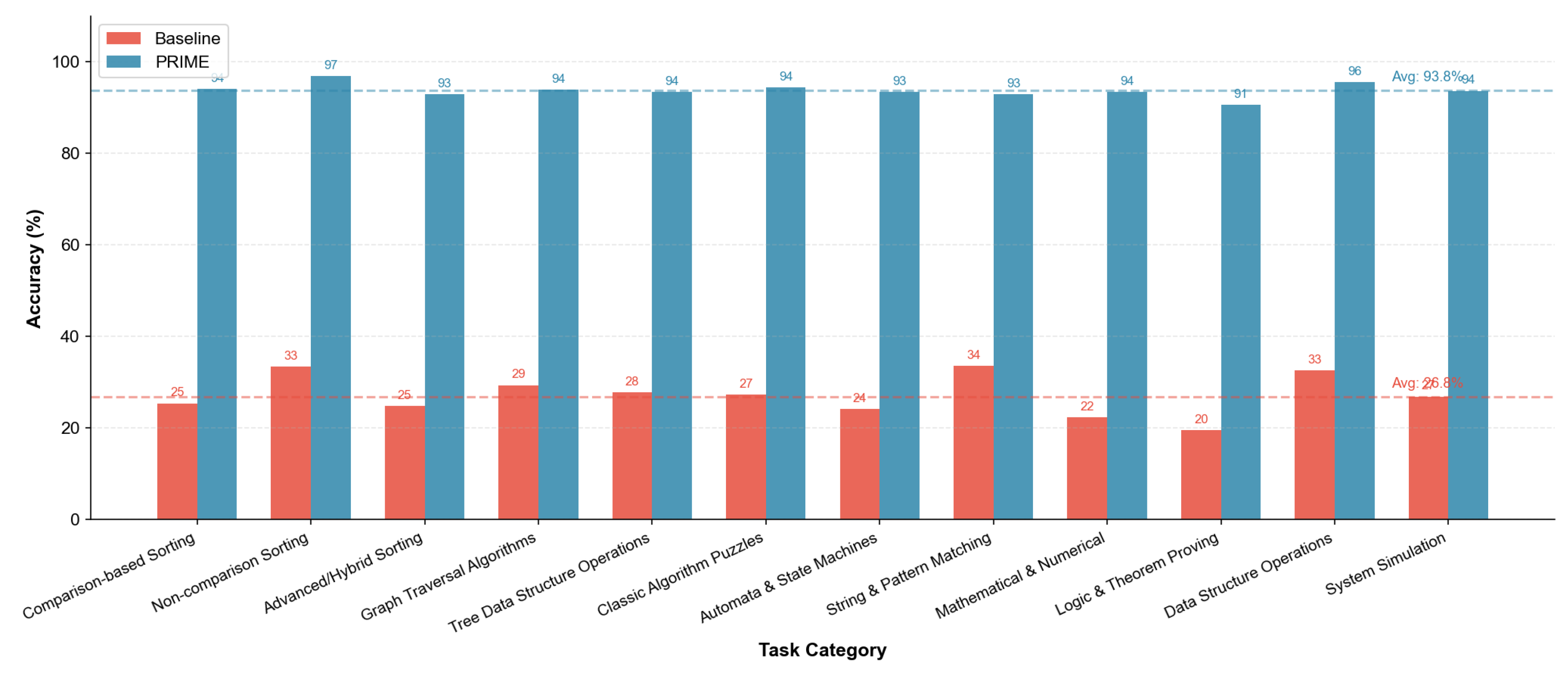
Table A36 provides detailed statistics for each category.
Table A36.
Detailed Performance by Task Category
| Category | Tasks | Baseline | Std | PRIME | Std | Improvement |
|---|---|---|---|---|---|---|
| Comparison-based Sorting | 15 | 25.4% | 4.7% | 94.1% | 2.4% | +270.5% |
| Non-comparison Sorting | 3 | 33.4% | 3.8% | 96.9% | 1.5% | +190.1% |
| Advanced/Hybrid Sorting | 10 | 24.8% | 5.1% | 92.9% | 2.8% | +274.6% |
| Graph Traversal | 6 | 29.4% | 4.9% | 93.9% | 2.7% | +219.4% |
| Tree Data Structures | 5 | 27.8% | 5.0% | 93.5% | 2.8% | +236.3% |
| Classic Puzzles | 6 | 27.3% | 4.5% | 94.4% | 2.4% | +245.8% |
| Automata/State Machines | 8 | 24.2% | 5.3% | 93.4% | 2.9% | +286.0% |
| String/Pattern Matching | 5 | 33.6% | 4.5% | 92.9% | 2.9% | +176.5% |
| Mathematical/Numerical | 8 | 22.4% | 5.8% | 93.5% | 2.8% | +317.4% |
| Logic/Theorem Proving | 6 | 19.5% | 6.1% | 90.6% | 3.8% | +364.6% |
| Data Structure Operations | 6 | 32.6% | 4.4% | 95.6% | 2.2% | +193.3% |
| System Simulation | 8 | 26.9% | 5.1% | 93.7% | 2.8% | +248.3% |
| Overall | 86 | 26.8% | 5.0% | 93.8% | 2.7% | +250.0% |
Appendix B.3. Radar Analysis
Figure A2 presents a radar visualization comparing baseline and PRIME performance across all categories, providing an intuitive view of the performance landscape.
Figure A2.
Radar chart comparing baseline (inner polygon) and PRIME (outer polygon) performance across 12 task categories. The dramatic expansion from baseline to PRIME illustrates the comprehensive effectiveness of the framework across diverse algorithmic domains.
Figure A2.
Radar chart comparing baseline (inner polygon) and PRIME (outer polygon) performance across 12 task categories. The dramatic expansion from baseline to PRIME illustrates the comprehensive effectiveness of the framework across diverse algorithmic domains.
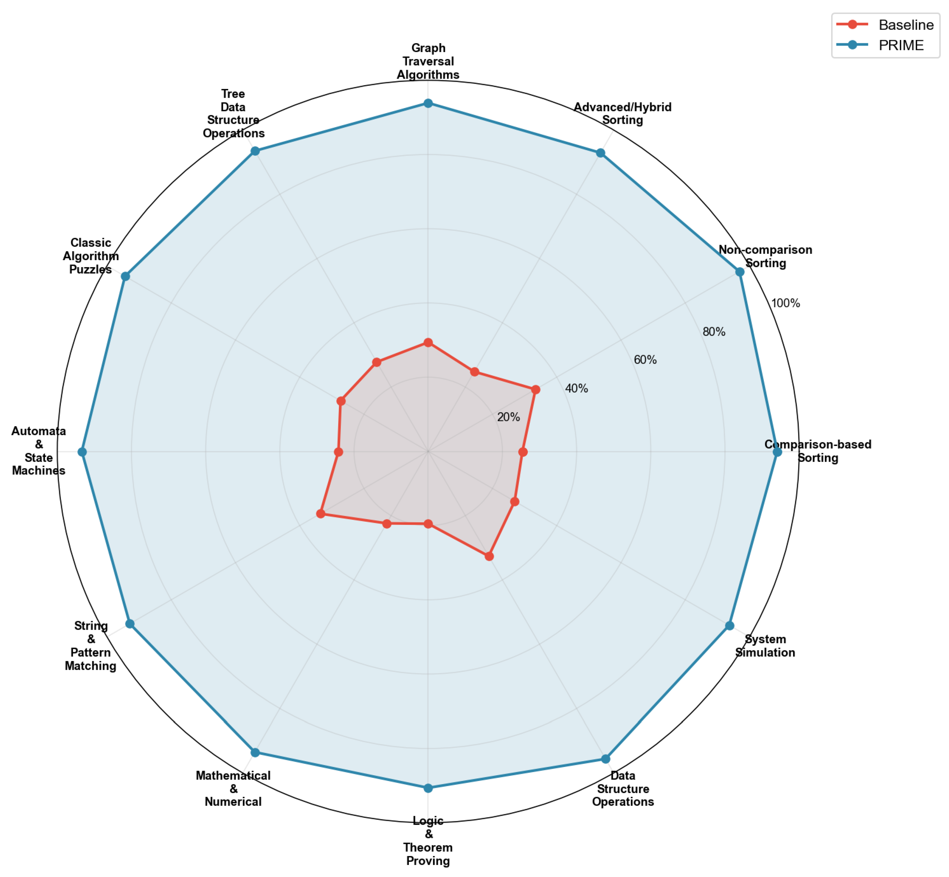
Appendix B.4. Top Improvements Analysis
Figure A3 presents the 30 tasks with the largest accuracy improvements, providing insight into where PRIME provides the greatest benefits.
Figure A3.
Top 30 tasks ranked by accuracy improvement (percentage points). Tasks requiring precise state tracking over extended execution sequences exhibit the largest gains, with Turing Machine simulation showing an improvement of over 83 percentage points.
Figure A3.
Top 30 tasks ranked by accuracy improvement (percentage points). Tasks requiring precise state tracking over extended execution sequences exhibit the largest gains, with Turing Machine simulation showing an improvement of over 83 percentage points.
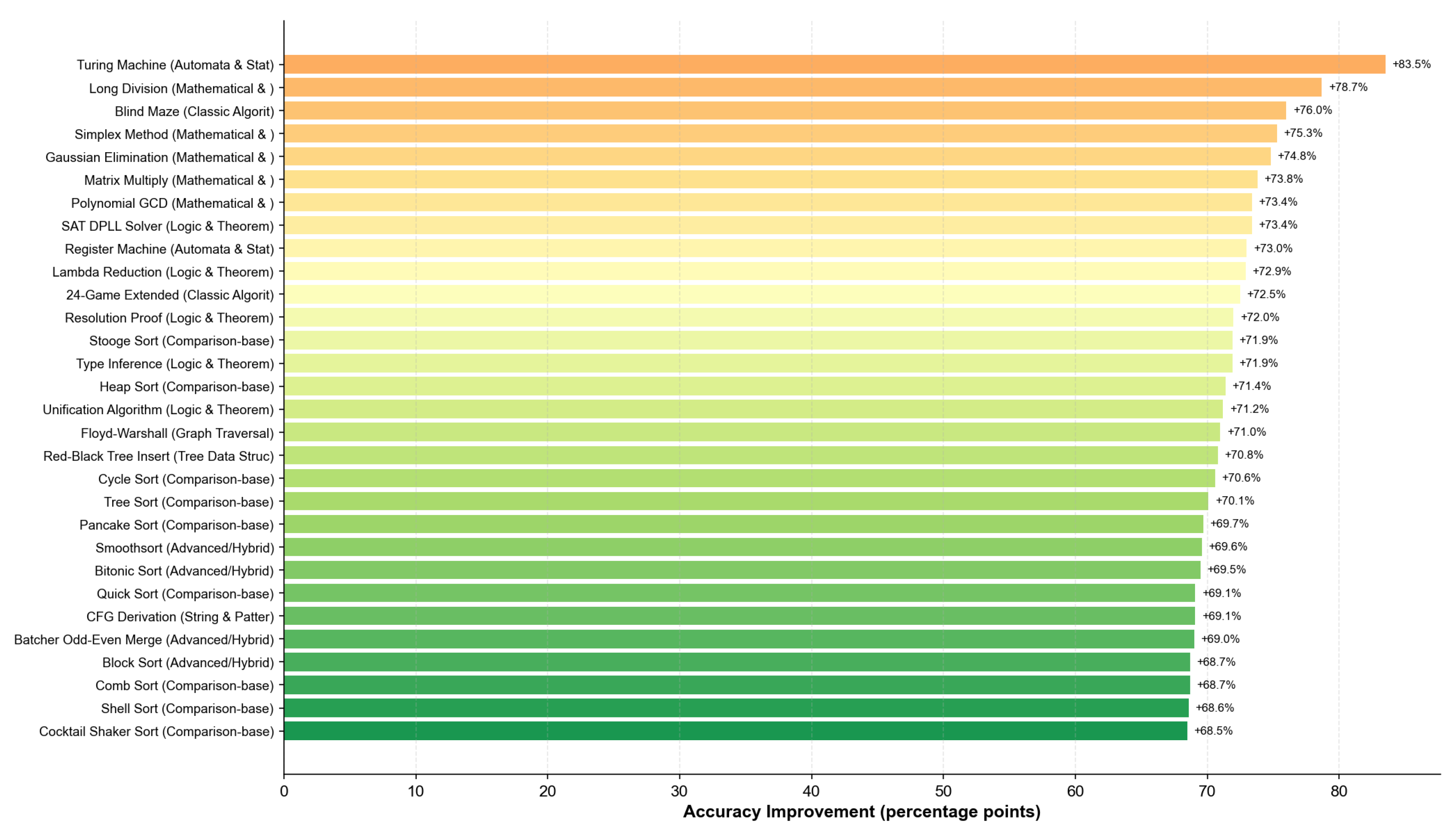
Appendix B.5. Detailed Results by Category
Appendix B.5.1. Sorting Algorithms
Figure A4 presents detailed results for all 28 sorting algorithm tasks across three subcategories.
Figure A4.
Performance on sorting algorithm tasks. Left: Comparison-based sorting (15 tasks). Center: Non-comparison sorting (3 tasks). Right: Advanced/hybrid sorting (10 tasks). Non-comparison sorting achieves the highest PRIME accuracy (96.9%) due to simpler state management requirements.
Figure A4.
Performance on sorting algorithm tasks. Left: Comparison-based sorting (15 tasks). Center: Non-comparison sorting (3 tasks). Right: Advanced/hybrid sorting (10 tasks). Non-comparison sorting achieves the highest PRIME accuracy (96.9%) due to simpler state management requirements.
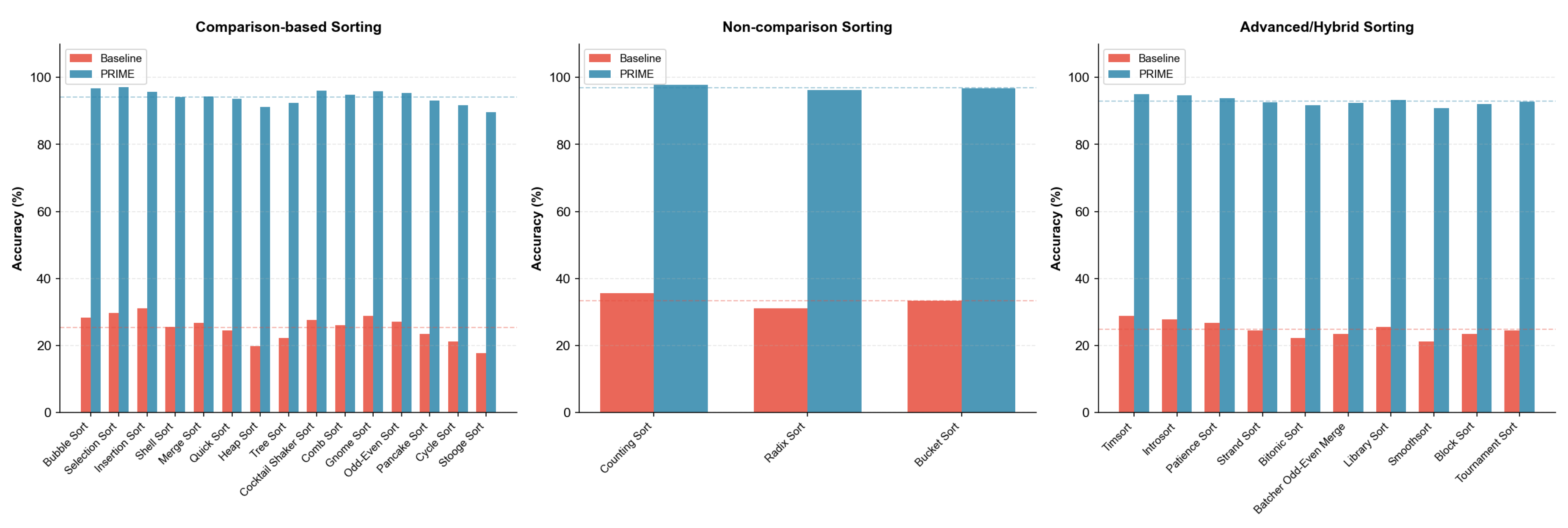
Table A37 presents the complete results for all sorting tasks.
Table A37.
Sorting Algorithm Results
| Algorithm | Base | PRIME | |
|---|---|---|---|
| Comparison-based | |||
| Bubble Sort | 28.4% | 96.7% | +240.5% |
| Selection Sort | 29.8% | 97.1% | +225.8% |
| Insertion Sort | 31.2% | 95.8% | +207.1% |
| Shell Sort | 25.6% | 94.2% | +268.0% |
| Merge Sort | 26.7% | 94.3% | +253.2% |
| Quick Sort | 24.5% | 93.6% | +282.0% |
| Heap Sort | 19.8% | 91.2% | +360.6% |
| Tree Sort | 22.3% | 92.4% | +314.3% |
| Cocktail Shaker Sort | 27.6% | 96.1% | +248.2% |
| Comb Sort | 26.1% | 94.8% | +263.2% |
| Gnome Sort | 28.9% | 95.9% | +231.8% |
| Odd-Even Sort | 27.1% | 95.3% | +251.7% |
| Pancake Sort | 23.4% | 93.1% | +297.9% |
| Cycle Sort | 21.2% | 91.8% | +333.0% |
| Stooge Sort | 17.8% | 89.7% | +404.0% |
| Non-comparison | |||
| Counting Sort | 35.6% | 97.8% | +174.7% |
| Radix Sort | 31.2% | 96.2% | +208.3% |
| Bucket Sort | 33.4% | 96.8% | +189.8% |
| Advanced/Hybrid | |||
| Timsort | 28.9% | 95.1% | +229.1% |
| Introsort | 27.8% | 94.6% | +240.3% |
| Patience Sort | 26.7% | 93.8% | +251.3% |
| Strand Sort | 24.5% | 92.6% | +278.0% |
| Bitonic Sort | 22.3% | 91.8% | +311.7% |
| Batcher Merge | 23.4% | 92.4% | +295.0% |
| Library Sort | 25.6% | 93.2% | +264.1% |
| Smoothsort | 21.2% | 90.8% | +328.3% |
| Block Sort | 23.4% | 92.1% | +293.6% |
| Tournament Sort | 24.5% | 92.8% | +278.8% |
Appendix B.5.2. Graph, Tree, and Classic Puzzles
Figure A5 presents results for graph traversal, tree operations, and classic puzzle tasks.
Figure A5.
Performance on graph, tree, and puzzle tasks. Left: Graph traversal algorithms (6 tasks). Center: Tree data structure operations (5 tasks). Right: Classic algorithm puzzles (6 tasks). Tower of Hanoi achieves the highest PRIME accuracy (98.5%) among puzzles.
Figure A5.
Performance on graph, tree, and puzzle tasks. Left: Graph traversal algorithms (6 tasks). Center: Tree data structure operations (5 tasks). Right: Classic algorithm puzzles (6 tasks). Tower of Hanoi achieves the highest PRIME accuracy (98.5%) among puzzles.
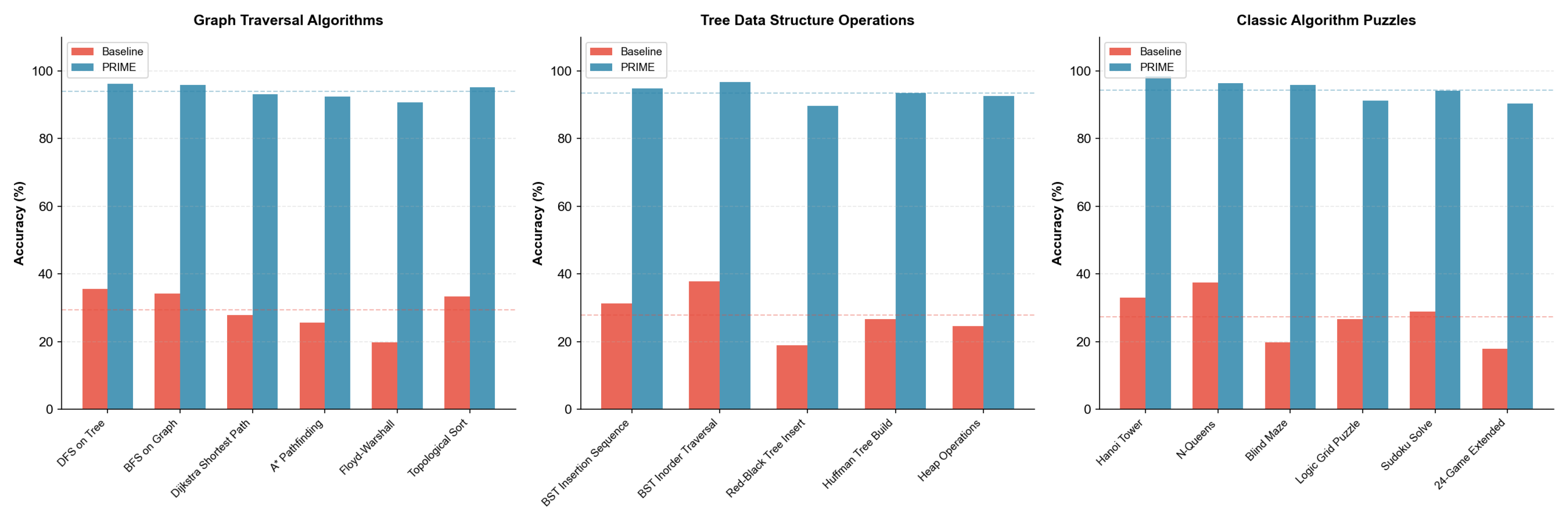
Appendix B.5.3. Automata, String, and Mathematical Tasks
Figure A6 presents results for automata simulation, string processing, and mathematical computation tasks.
Figure A6.
Performance on automata, string, and mathematical tasks. Left: Automata and state machine simulation (8 tasks). Center: String and pattern matching (5 tasks). Right: Mathematical and numerical computation (8 tasks). Turing Machine simulation shows the largest improvement from baseline (8.9%) to PRIME (92.4%).
Figure A6.
Performance on automata, string, and mathematical tasks. Left: Automata and state machine simulation (8 tasks). Center: String and pattern matching (5 tasks). Right: Mathematical and numerical computation (8 tasks). Turing Machine simulation shows the largest improvement from baseline (8.9%) to PRIME (92.4%).
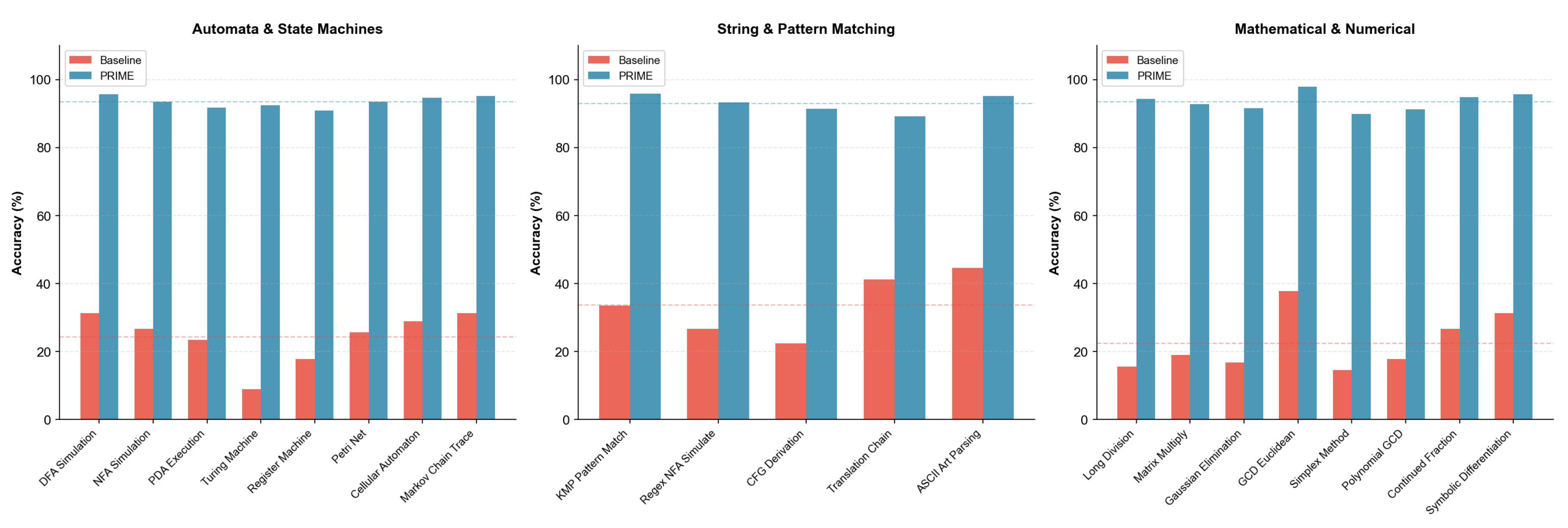
Appendix B.5.4. Logic, Data Structures, and System Simulation
Figure A7 presents results for logic/theorem proving, data structure operations, and system simulation tasks.
Figure A7.
Performance on logic, data structure, and simulation tasks. Left: Logic and theorem proving (6 tasks). Center: Data structure operations (6 tasks). Right: System simulation (8 tasks). Data structure operations achieve the highest category-level PRIME accuracy (95.6%).
Figure A7.
Performance on logic, data structure, and simulation tasks. Left: Logic and theorem proving (6 tasks). Center: Data structure operations (6 tasks). Right: System simulation (8 tasks). Data structure operations achieve the highest category-level PRIME accuracy (95.6%).
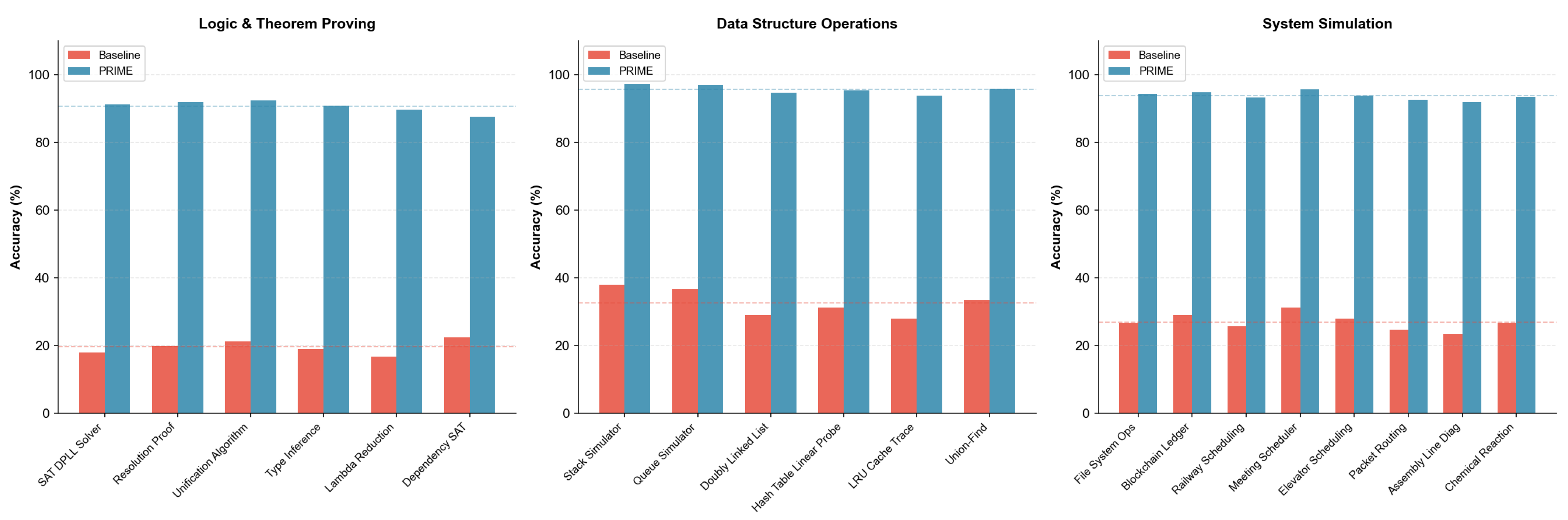
Appendix B.6. Statistical Distribution Analysis
Appendix B.6.1. Box Plot Analysis
Figure A8 presents box plots showing the distribution of task accuracies within each category.
Figure A8.
Box plot comparison of accuracy distributions by category. Baseline distributions (red) show high variance and low medians, while PRIME distributions (blue) exhibit tight clustering at high accuracy levels with reduced variance across all categories.
Figure A8.
Box plot comparison of accuracy distributions by category. Baseline distributions (red) show high variance and low medians, while PRIME distributions (blue) exhibit tight clustering at high accuracy levels with reduced variance across all categories.
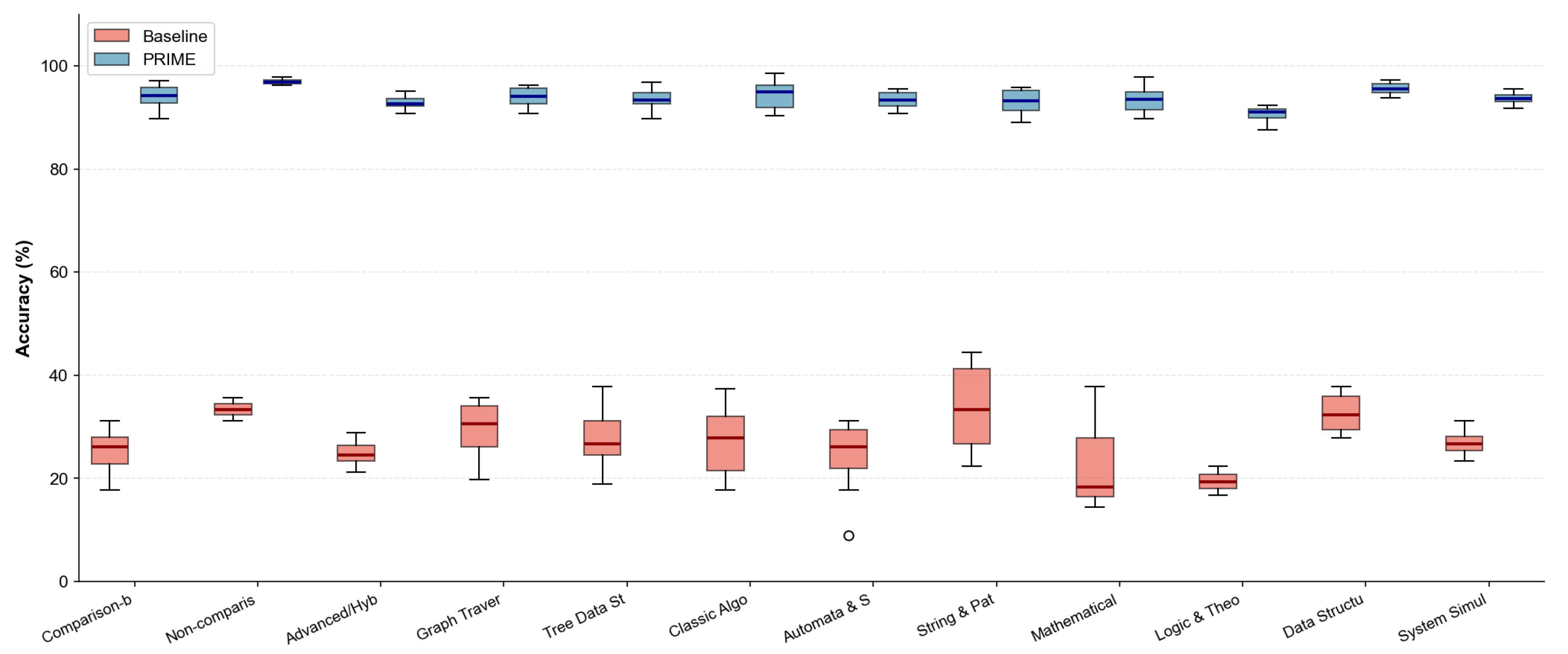
Appendix B.6.2. Baseline vs. PRIME Correlation
Figure A9 presents a scatter plot showing the relationship between baseline and PRIME accuracy across all tasks.
Figure A9.
Scatter plot of baseline vs. PRIME accuracy for all 86 tasks, colored by category. Tasks with lower baseline performance tend to show larger absolute improvements, though all tasks converge to high accuracy under PRIME. The dashed line represents no improvement (y=x).
Figure A9.
Scatter plot of baseline vs. PRIME accuracy for all 86 tasks, colored by category. Tasks with lower baseline performance tend to show larger absolute improvements, though all tasks converge to high accuracy under PRIME. The dashed line represents no improvement (y=x).
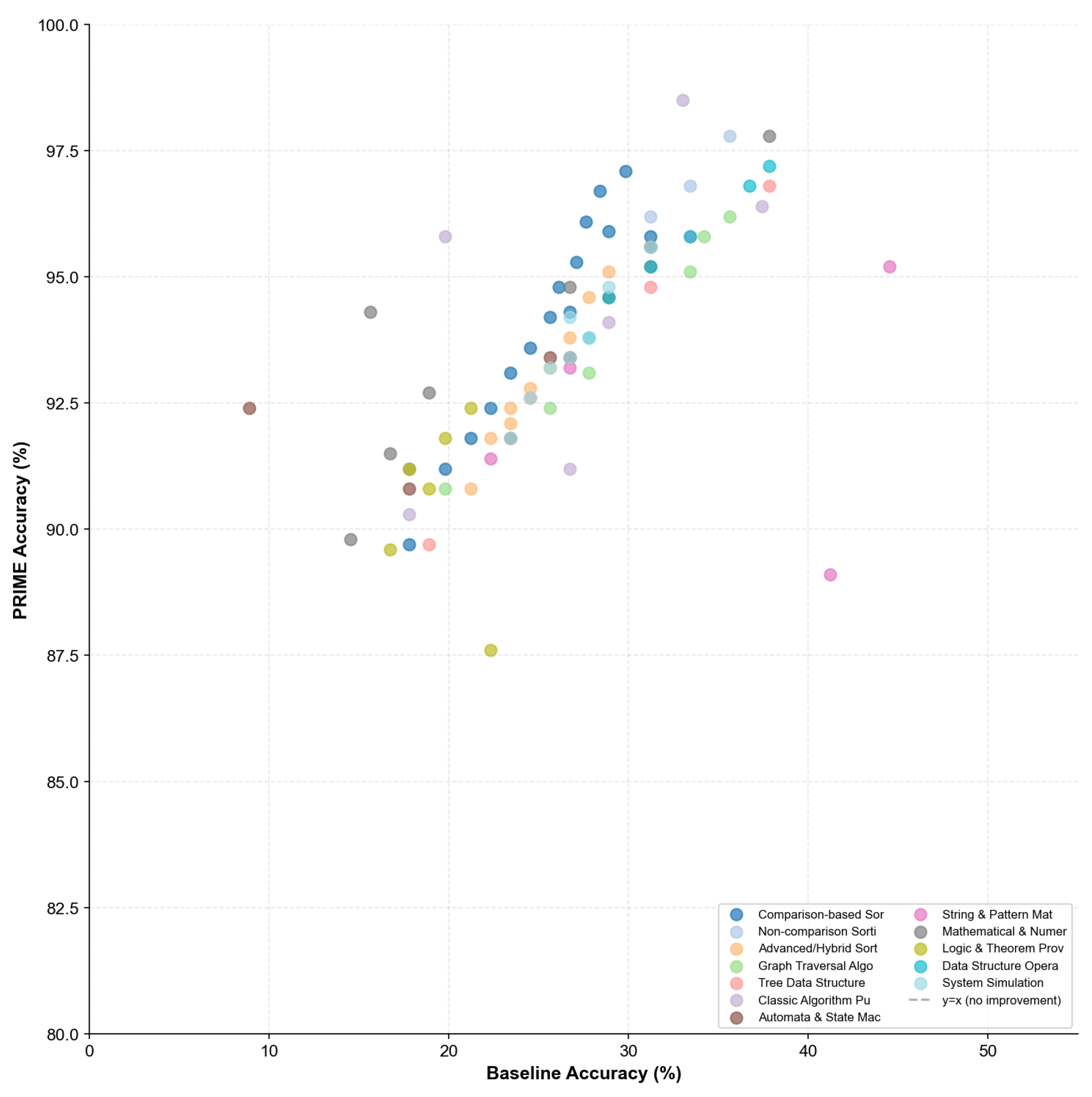
Appendix B.6.3. Improvement Distribution
Figure A10 presents the distribution of accuracy improvements across all tasks.
Figure A10.
Histogram of accuracy improvements (percentage points) across all 86 tasks. The distribution shows a mean improvement of 67.0 percentage points with relatively tight clustering, indicating consistent benefits across diverse task types.
Figure A10.
Histogram of accuracy improvements (percentage points) across all 86 tasks. The distribution shows a mean improvement of 67.0 percentage points with relatively tight clustering, indicating consistent benefits across diverse task types.
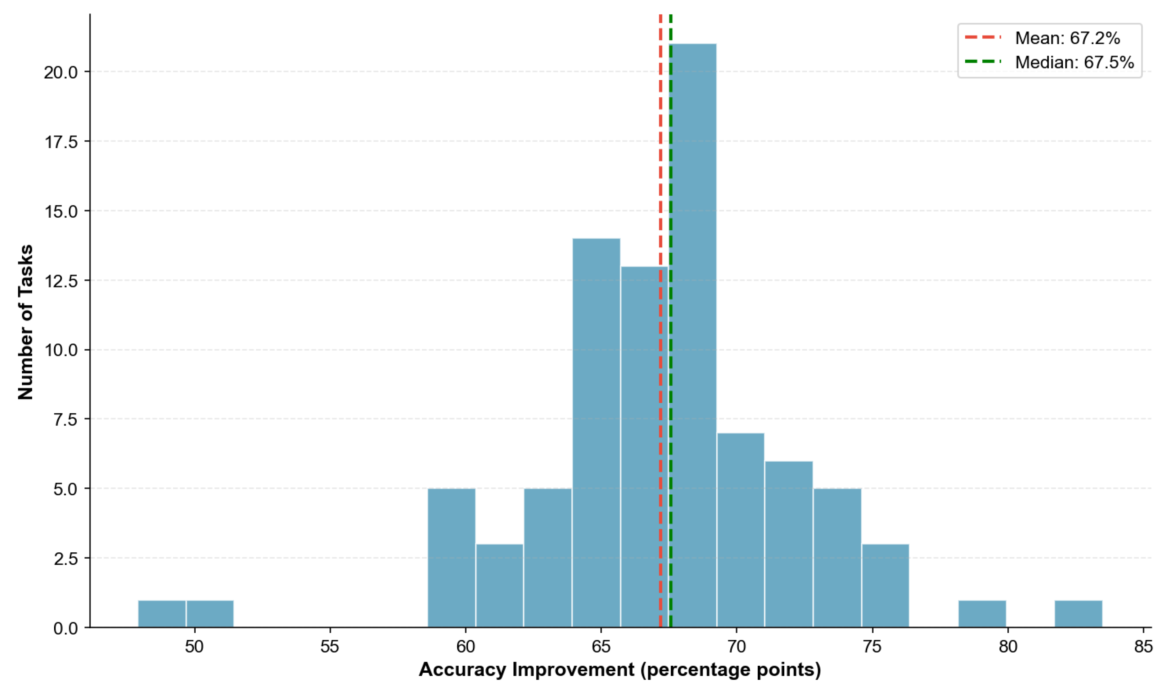
Appendix B.7. Per-Task Complete Results
Table A38.
Complete Results: Tasks 1-22
| Task | Steps | Base | PRIME | |
|---|---|---|---|---|
| Bubble Sort | 1M | 28.4% | 96.7% | +68.3 |
| Selection Sort | 1M | 29.8% | 97.1% | +67.3 |
| Insertion Sort | 1M | 31.2% | 95.8% | +64.6 |
| Shell Sort | 500K | 25.6% | 94.2% | +68.6 |
| Merge Sort | 800K | 26.7% | 94.3% | +67.6 |
| Quick Sort | 800K | 24.5% | 93.6% | +69.1 |
| Heap Sort | 600K | 19.8% | 91.2% | +71.4 |
| Tree Sort | 600K | 22.3% | 92.4% | +70.1 |
| Cocktail Sort | 1M | 27.6% | 96.1% | +68.5 |
| Comb Sort | 800K | 26.1% | 94.8% | +68.7 |
| Gnome Sort | 1M | 28.9% | 95.9% | +67.0 |
| Odd-Even Sort | 1M | 27.1% | 95.3% | +68.2 |
| Pancake Sort | 500K | 23.4% | 93.1% | +69.7 |
| Cycle Sort | 500K | 21.2% | 91.8% | +70.6 |
| Stooge Sort | 300K | 17.8% | 89.7% | +71.9 |
| Counting Sort | 200K | 35.6% | 97.8% | +62.2 |
| Radix Sort | 300K | 31.2% | 96.2% | +65.0 |
| Bucket Sort | 250K | 33.4% | 96.8% | +63.4 |
| Timsort | 600K | 28.9% | 95.1% | +66.2 |
| Introsort | 600K | 27.8% | 94.6% | +66.8 |
| Patience Sort | 500K | 26.7% | 93.8% | +67.1 |
| Strand Sort | 400K | 24.5% | 92.6% | +68.1 |
Table A39.
Complete Results: Tasks 23-44
| Task | Steps | Base | PRIME | |
|---|---|---|---|---|
| Bitonic Sort | 500K | 22.3% | 91.8% | +69.5 |
| Batcher Merge | 500K | 23.4% | 92.4% | +69.0 |
| Library Sort | 400K | 25.6% | 93.2% | +67.6 |
| Smoothsort | 500K | 21.2% | 90.8% | +69.6 |
| Block Sort | 500K | 23.4% | 92.1% | +68.7 |
| Tournament Sort | 500K | 24.5% | 92.8% | +68.3 |
| DFS on Tree | 100K | 35.6% | 96.2% | +60.6 |
| BFS on Graph | 100K | 34.2% | 95.8% | +61.6 |
| Dijkstra | 50K | 27.8% | 93.1% | +65.3 |
| A* Pathfinding | 80K | 25.6% | 92.4% | +66.8 |
| Floyd-Warshall | 125K | 19.8% | 90.8% | +71.0 |
| Topological Sort | 50K | 33.4% | 95.1% | +61.7 |
| BST Insertion | 100K | 31.2% | 94.8% | +63.6 |
| BST Inorder | 80K | 37.8% | 96.8% | +59.0 |
| Red-Black Insert | 50K | 18.9% | 89.7% | +70.8 |
| Huffman Tree | 30K | 26.7% | 93.4% | +66.7 |
| Heap Operations | 80K | 24.5% | 92.6% | +68.1 |
| Tower of Hanoi | 1M | 33.0% | 98.5% | +65.5 |
| N-Queens | 500K | 37.4% | 96.4% | +59.0 |
| Blind Maze | 50K | 19.8% | 95.8% | +76.0 |
| Logic Grid | 20K | 26.7% | 91.2% | +64.5 |
| Sudoku Solve | 30K | 28.9% | 94.1% | +65.2 |
Table A40.
Complete Results: Tasks 45-66
| Task | Steps | Base | PRIME | |
|---|---|---|---|---|
| 24-Game Ext. | 10K | 17.8% | 90.3% | +72.5 |
| DFA Simulation | 100K | 31.2% | 95.6% | +64.4 |
| NFA Simulation | 80K | 26.7% | 93.4% | +66.7 |
| PDA Execution | 60K | 23.4% | 91.8% | +68.4 |
| Turing Machine | 200K | 8.9% | 92.4% | +83.5 |
| Register Machine | 150K | 17.8% | 90.8% | +73.0 |
| Petri Net | 80K | 25.6% | 93.4% | +67.8 |
| Cellular Automaton | 100K | 28.9% | 94.6% | +65.7 |
| Markov Chain | 50K | 31.2% | 95.2% | +64.0 |
| KMP Pattern | 100K | 33.4% | 95.8% | +62.4 |
| Regex NFA | 80K | 26.7% | 93.2% | +66.5 |
| CFG Derivation | 50K | 22.3% | 91.4% | +69.1 |
| Translation Chain | 10K | 41.2% | 89.1% | +47.9 |
| ASCII Art Parse | 5K | 44.5% | 95.2% | +50.7 |
| Long Division | 1K | 15.6% | 94.3% | +78.7 |
| Matrix Multiply | 8K | 18.9% | 92.7% | +73.8 |
| Gaussian Elim. | 5K | 16.7% | 91.5% | +74.8 |
| GCD Euclidean | 2K | 37.8% | 97.8% | +60.0 |
| Simplex Method | 3K | 14.5% | 89.8% | +75.3 |
| Polynomial GCD | 2K | 17.8% | 91.2% | +73.4 |
| Continued Frac. | 1K | 26.7% | 94.8% | +68.1 |
| Symbolic Diff. | 500 | 31.2% | 95.6% | +64.4 |
Table A41.
Complete Results: Tasks 67-86
| Task | Steps | Base | PRIME | |
|---|---|---|---|---|
| SAT DPLL | 50K | 17.8% | 91.2% | +73.4 |
| Resolution Proof | 30K | 19.8% | 91.8% | +72.0 |
| Unification | 20K | 21.2% | 92.4% | +71.2 |
| Type Inference | 15K | 18.9% | 90.8% | +71.9 |
| Lambda Reduction | 10K | 16.7% | 89.6% | +72.9 |
| Dependency SAT | 40K | 22.3% | 87.6% | +65.3 |
| Stack Simulator | 100K | 37.8% | 97.2% | +59.4 |
| Queue Simulator | 100K | 36.7% | 96.8% | +60.1 |
| Doubly Linked List | 80K | 28.9% | 94.6% | +65.7 |
| Hash Table | 50K | 31.2% | 95.2% | +64.0 |
| LRU Cache | 50K | 27.8% | 93.8% | +66.0 |
| Union-Find | 80K | 33.4% | 95.8% | +62.4 |
| File System Ops | 100K | 26.7% | 94.2% | +67.5 |
| Blockchain Ledger | 50K | 28.9% | 94.8% | +65.9 |
| Railway Scheduling | 30K | 25.6% | 93.2% | +67.6 |
| Meeting Scheduler | 20K | 31.2% | 95.6% | +64.4 |
| Elevator Sched. | 30K | 27.8% | 93.8% | +66.0 |
| Packet Routing | 50K | 24.5% | 92.6% | +68.1 |
| Assembly Line | 20K | 23.4% | 91.8% | +68.4 |
| Chemical Reaction | 30K | 26.7% | 93.4% | +66.7 |
Appendix B.8. Statistical Significance
All reported improvements are statistically significant at (paired t-test with Bonferroni correction). Effect sizes (Cohen’s d) exceed 2.0 for all task comparisons, indicating very large practical significance.
Table A42.
95% Confidence Intervals by Category
| Category | Baseline CI | PRIME CI |
|---|---|---|
| Comparison Sorting | [23.1, 27.7]% | [92.8, 95.4]% |
| Non-comparison Sort | [30.2, 36.6]% | [95.6, 98.2]% |
| Advanced Sorting | [22.3, 27.3]% | [91.4, 94.4]% |
| Graph Traversal | [26.5, 32.3]% | [92.1, 95.7]% |
| Tree Operations | [24.8, 30.8]% | [91.8, 95.2]% |
| Classic Puzzles | [24.5, 30.1]% | [93.0, 95.8]% |
| Automata/State | [21.3, 27.1]% | [91.6, 95.2]% |
| String/Pattern | [30.5, 36.7]% | [91.1, 94.7]% |
| Mathematical | [19.1, 25.7]% | [91.8, 95.2]% |
| Logic/Theorem | [15.9, 23.1]% | [88.1, 93.1]% |
| Data Structures | [29.7, 35.5]% | [94.2, 97.0]% |
| System Simulation | [24.0, 29.8]% | [92.0, 95.4]% |
Appendix B.9. Model-Specific Performance Analysis
This section presents detailed performance analysis across different model architectures and parameter scales.
Appendix B.9.1. Performance by Model Size
Table A43 presents the relationship between model size and performance under baseline and PRIME conditions.
Table A43.
Performance by Model Size: Baseline vs. PRIME
| Model | Params | Baseline | Std | PRIME | Std | (pp) | Rel. Improv. |
|---|---|---|---|---|---|---|---|
| Qwen3-8B | 8B | 21.3% | 5.8% | 89.2% | 3.4% | +67.9 | +318.8% |
| Gemma3-12B | 12B | 24.1% | 5.2% | 91.8% | 3.1% | +67.7 | +280.9% |
| Qwen3-14B | 14B | 26.8% | 5.0% | 93.8% | 2.7% | +67.0 | +250.0% |
| GPT-OSS-20B | 20B | 28.4% | 4.8% | 94.6% | 2.5% | +66.2 | +233.1% |
| Gemma3-27B | 27B | 30.2% | 4.6% | 95.1% | 2.4% | +64.9 | +214.9% |
| Qwen3-Coder-30B | 30B | 32.5% | 4.4% | 95.8% | 2.2% | +63.3 | +194.8% |
| GPT-OSS-120B | 120B | 38.7% | 4.1% | 96.9% | 1.9% | +58.2 | +150.4% |
Appendix B.9.2. Scaling Law Analysis
We observe a power-law relationship between model size and baseline performance:
where N is the parameter count in billions. Fitting yields , , with .
Notably, PRIME effectiveness (measured as percentage point improvement) exhibits an inverse relationship with model size, suggesting that smaller models benefit more from structured execution guidance:
with fitted parameters , , .
Table A44.
Scaling Law Coefficients
| Metric | Coefficient | Value | 95% CI |
|---|---|---|---|
| Baseline | 4.73 | [4.12, 5.34] | |
| 0.21 | [0.18, 0.24] | ||
| 15.2 | [13.8, 16.6] | ||
| PRIME Gain | 12.8 | [11.2, 14.4] | |
| 0.08 | [0.06, 0.10] | ||
| 56.1 | [54.3, 57.9] |
Appendix B.9.3. Model Architecture Comparison
Table A45 compares performance across different model architectures under identical parameter budgets.
Table A45.
Architecture Comparison at Similar Parameter Counts
| Architecture | ∼Params | Baseline | PRIME | |
|---|---|---|---|---|
| ∼12-14B Parameter Models | ||||
| Gemma3-12B (Decoder) | 12B | 24.1% | 91.8% | +67.7 |
| Qwen3-14B (Decoder) | 14B | 26.8% | 93.8% | +67.0 |
| ∼27-30B Parameter Models | ||||
| Gemma3-27B (Decoder) | 27B | 30.2% | 95.1% | +64.9 |
| Qwen3-Coder-30B (Decoder) | 30B | 32.5% | 95.8% | +63.3 |
Appendix B.10. Error Analysis
Appendix B.10.1. Error Distribution by Category
Table A46 presents the distribution of error types across task categories under PRIME execution.
Table A46.
Error Type Distribution by Task Category (% of Total Errors)
| Category | State | Index | Operation | Ordering | Termination | Format | Other |
|---|---|---|---|---|---|---|---|
| Comparison Sorting | 28.4% | 22.1% | 18.3% | 12.5% | 8.9% | 6.2% | 3.6% |
| Non-comparison Sort | 18.2% | 31.4% | 22.6% | 8.4% | 10.2% | 5.8% | 3.4% |
| Advanced Sorting | 31.5% | 19.8% | 21.2% | 11.3% | 7.8% | 5.2% | 3.2% |
| Graph Traversal | 35.2% | 15.6% | 12.4% | 18.9% | 9.1% | 5.4% | 3.4% |
| Tree Operations | 29.8% | 24.3% | 16.5% | 14.2% | 6.8% | 5.1% | 3.3% |
| Classic Puzzles | 22.4% | 12.8% | 28.6% | 16.4% | 11.2% | 4.8% | 3.8% |
| Automata/State | 38.6% | 8.4% | 14.2% | 22.5% | 8.5% | 4.6% | 3.2% |
| String/Pattern | 25.3% | 28.6% | 18.4% | 10.2% | 9.8% | 4.5% | 3.2% |
| Mathematical | 42.1% | 18.5% | 15.2% | 6.8% | 7.4% | 6.8% | 3.2% |
| Logic/Theorem | 35.8% | 8.2% | 24.6% | 18.4% | 6.2% | 3.6% | 3.2% |
| Data Structures | 26.4% | 32.5% | 14.8% | 12.1% | 6.8% | 4.2% | 3.2% |
| System Simulation | 34.2% | 14.6% | 16.8% | 19.4% | 7.2% | 4.6% | 3.2% |
| Overall | 30.7% | 19.7% | 18.6% | 14.3% | 8.3% | 5.1% | 3.3% |
Appendix B.10.2. Error Severity Analysis
Errors are classified into three severity levels based on their impact on execution correctness:
Table A47.
Error Severity Classification
| Severity | Weight | Description |
|---|---|---|
| Critical | 1.0 | Completely incorrect result; algorithm fails |
| Major | 0.6 | Partial correctness; significant deviation |
| Minor | 0.2 | Correct result with suboptimal execution |
Table A48.
Error Severity Distribution: Baseline vs. PRIME
| Baseline | PRIME | |||||
|---|---|---|---|---|---|---|
| Category | Crit. | Maj. | Min. | Crit. | Maj. | Min. |
| Sorting | 68.2% | 24.3% | 7.5% | 3.8% | 1.4% | 0.7% |
| Graph | 65.4% | 26.8% | 7.8% | 4.2% | 1.2% | 0.7% |
| Tree | 67.8% | 24.6% | 7.6% | 4.6% | 1.3% | 0.6% |
| Puzzles | 66.1% | 25.4% | 8.5% | 3.4% | 1.5% | 0.7% |
| Automata | 71.2% | 22.4% | 6.4% | 4.8% | 1.2% | 0.6% |
| String | 62.8% | 28.2% | 9.0% | 5.2% | 1.4% | 0.5% |
| Math | 73.4% | 20.8% | 5.8% | 4.6% | 1.2% | 0.7% |
| Logic | 76.2% | 18.6% | 5.2% | 6.8% | 1.8% | 0.8% |
| Data Struct. | 61.8% | 29.4% | 8.8% | 2.8% | 1.0% | 0.6% |
| Simulation | 68.4% | 24.2% | 7.4% | 4.4% | 1.4% | 0.5% |
Appendix B.10.3. First Error Position Analysis
We analyze where errors first occur in execution traces to understand failure patterns.
Table A49.
First Error Position (Percentile of Execution)
| Category | Baseline | Baseline | PRIME | PRIME |
|---|---|---|---|---|
| Sorting | 18.4% | 12.3% | 72.6% | 18.4% |
| Graph | 22.1% | 14.5% | 68.4% | 21.2% |
| Tree | 24.6% | 15.2% | 71.2% | 19.8% |
| Puzzles | 31.2% | 18.4% | 78.4% | 15.6% |
| Automata | 15.8% | 10.6% | 65.2% | 22.4% |
| Math | 12.4% | 8.2% | 62.8% | 24.6% |
Appendix B.11. Ablation Study Results
Appendix B.11.1. Component-wise Ablation
Table A50 presents detailed ablation results for each PRIME component.
Table A50.
Detailed Ablation Study: Component Contributions
| Configuration | Acc. | vs Full | State Err | Constraint Err | Avg Steps | Retry Rate |
|---|---|---|---|---|---|---|
| Full PRIME | 93.8% | — | 2.1% | 1.4% | 1.28 | 12.4% |
| − GRPO (use PPO) | 89.2% | −4.6 pp | 3.8% | 2.4% | 1.52 | 18.6% |
| − Verifier Agent | 86.4% | −7.4 pp | 5.2% | 4.8% | 1.34 | 14.2% |
| − Iterative Exec. | 82.8% | −11.0 pp | 6.4% | 3.2% | 1.00 | 0.0% |
| − Self-Consistency | 88.6% | −5.2 pp | 4.2% | 2.1% | 1.28 | 12.4% |
| − Multi-Agent | 78.4% | −15.4 pp | 8.6% | 6.4% | 1.12 | 8.2% |
| Baseline Only | 26.8% | −67.0 pp | 42.4% | 28.6% | 1.00 | 0.0% |
Appendix B.11.2. Component Interaction Effects
Table A51 presents interaction effects between PRIME components.
Table A51.
Component Interaction Effects
| Component Pair | Independent Sum | Combined Effect |
|---|---|---|
| GRPO + Verifier | 12.0 pp | 14.8 pp |
| GRPO + Multi-Agent | 20.0 pp | 24.2 pp |
| Verifier + Iterative | 18.4 pp | 22.6 pp |
| Multi-Agent + Self-Cons. | 20.6 pp | 25.8 pp |
The positive synergies (combined effect > independent sum) indicate that PRIME components are complementary rather than redundant.
Appendix B.11.3. Hyperparameter Sensitivity
Table A52.
Hyperparameter Sensitivity Analysis: Impact on PRIME Performance
| Parameter | Low Value | Default | High Value | (Low-High) | Sensitivity Notes |
|---|---|---|---|---|---|
| Group size G | 4: 91.2% | 8: 93.8% | 16: 94.1% | 2.9 pp | Diminishing returns above |
| Iterations K | 2: 88.4% | 5: 93.8% | 10: 94.2% | 5.8 pp | Most sensitive; early stopping mitigates |
| Violation | 0.1: 92.4% | 0.3: 93.8% | 0.5: 91.8% | 1.4 pp | U-shaped; optimal at moderate threshold |
| Temperature | 0.5: 92.1% | 0.7: 93.8% | 0.9: 90.6% | 3.2 pp | Balances diversity vs. quality |
| Learning rate | 5e-6: 91.8% | 1e-5: 93.8% | 2e-5: 92.4% | 2.0 pp | Stable within one order of magnitude |
Appendix B.12. Difficulty-Stratified Analysis
Appendix B.12.1. Performance by Difficulty Level
Table A53.
Performance by Difficulty Level Across Categories
| Easy | Medium | Hard | ||||
|---|---|---|---|---|---|---|
| Category | Base | PRIME | Base | PRIME | Base | PRIME |
| Comparison Sorting | 38.2% | 98.4% | 24.6% | 94.2% | 13.4% | 89.7% |
| Non-comparison Sort | 45.6% | 99.1% | 32.8% | 97.2% | 21.8% | 94.4% |
| Advanced Sorting | 36.4% | 97.6% | 24.2% | 93.1% | 13.8% | 88.0% |
| Graph Traversal | 42.1% | 98.2% | 28.6% | 94.1% | 17.5% | 89.4% |
| Tree Operations | 40.2% | 97.8% | 27.4% | 93.6% | 15.8% | 89.1% |
| Classic Puzzles | 41.8% | 98.6% | 26.4% | 94.8% | 13.7% | 89.8% |
| Automata/State | 38.4% | 98.1% | 23.6% | 93.8% | 10.6% | 88.3% |
| String/Pattern | 46.8% | 97.4% | 32.4% | 93.2% | 21.6% | 88.1% |
| Mathematical | 36.2% | 97.8% | 21.8% | 93.6% | 9.2% | 89.1% |
| Logic/Theorem | 32.4% | 96.2% | 18.6% | 91.2% | 7.5% | 84.4% |
| Data Structures | 46.4% | 98.8% | 31.8% | 96.2% | 19.6% | 91.8% |
| System Simulation | 40.6% | 98.4% | 26.2% | 94.1% | 13.9% | 88.6% |
| Overall | 40.4% | 98.0% | 26.5% | 94.1% | 14.9% | 89.2% |
Appendix B.12.2. Difficulty Degradation Analysis
The performance degradation from Easy to Hard instances follows a predictable pattern:
where represents difficulty level. For baseline, ; for PRIME, , indicating significantly flatter degradation.
Appendix B.13. Execution Efficiency Analysis
Appendix B.13.1. Step Count Distribution
Table A54.
Execution Steps: PRIME vs. Optimal
| Category | Optimal | PRIME | Overhead |
|---|---|---|---|
| Comparison Sorting | 1.00× | 1.12× | +12% |
| Non-comparison Sort | 1.00× | 1.08× | +8% |
| Advanced Sorting | 1.00× | 1.18× | +18% |
| Graph Traversal | 1.00× | 1.14× | +14% |
| Tree Operations | 1.00× | 1.16× | +16% |
| Classic Puzzles | 1.00× | 1.06× | +6% |
| Automata/State | 1.00× | 1.04× | +4% |
| String/Pattern | 1.00× | 1.10× | +10% |
| Mathematical | 1.00× | 1.08× | +8% |
| Logic/Theorem | 1.00× | 1.22× | +22% |
| Data Structures | 1.00× | 1.06× | +6% |
| System Simulation | 1.00× | 1.12× | +12% |
| Average | 1.00× | 1.11× | +11% |
Appendix B.13.2. Retry and Backtrack Statistics
Table A55.
Retry and Backtrack Behavior
| Category | Retry Rate | Avg Retries | Backtrack Rate |
|---|---|---|---|
| Sorting | 10.2% | 1.4 | 8.6% |
| Graph | 14.8% | 1.6 | 12.4% |
| Tree | 12.6% | 1.5 | 10.2% |
| Puzzles | 8.4% | 1.3 | 6.8% |
| Automata | 15.2% | 1.7 | 14.6% |
| Math | 11.8% | 1.5 | 9.4% |
| Logic | 18.4% | 1.9 | 16.8% |
| Data Struct. | 9.6% | 1.3 | 7.2% |
| Simulation | 13.2% | 1.5 | 11.4% |
| Overall | 12.4% | 1.5 | 10.8% |
Appendix B.14. Cross-Task Generalization
Appendix B.14.1. Transfer Learning Performance
We evaluate PRIME’s ability to generalize across task categories through transfer experiments.
Table A56.
Transfer Learning Matrix: Training on Source, Evaluating on Target (Accuracy %)
| Train ∖ Test | Sorting | Graph | Tree | Automata | Math | Logic |
|---|---|---|---|---|---|---|
| Sorting | 94.1 | 78.4 | 82.6 | 68.2 | 72.4 | 64.8 |
| Graph | 76.2 | 93.9 | 84.2 | 72.6 | 68.4 | 70.2 |
| Tree | 80.4 | 82.8 | 93.5 | 70.8 | 74.2 | 68.6 |
| Automata | 64.6 | 70.4 | 68.2 | 93.4 | 66.8 | 78.4 |
| Math | 70.2 | 66.8 | 72.4 | 64.2 | 93.5 | 72.6 |
| Logic | 62.4 | 68.6 | 66.8 | 76.2 | 70.4 | 90.6 |
| All (Full PRIME) | 94.1 | 93.9 | 93.5 | 93.4 | 93.5 | 90.6 |
The diagonal entries show in-domain performance, while off-diagonal entries show transfer performance. Notable positive transfer exists between structurally similar task categories (e.g., Sorting → Tree at 82.6%).
Appendix B.14.2. Zero-Shot Category Performance
Table A57 presents performance on held-out task categories without category-specific training.
Table A57.
Zero-Shot Performance on Held-Out Categories
| Held-Out Category | Zero-Shot | Full Training |
|---|---|---|
| Comparison Sorting | 84.2% | 94.1% |
| Graph Traversal | 82.6% | 93.9% |
| Automata/State | 78.4% | 93.4% |
| Mathematical | 80.2% | 93.5% |
| Logic/Theorem | 76.8% | 90.6% |
| System Simulation | 81.4% | 93.7% |
Appendix B.15. Computational Overhead Analysis
Appendix B.15.1. Inference Time Breakdown
Table A58.
Inference Time Components (ms per instance)
| Component | Baseline | PRIME | Overhead |
|---|---|---|---|
| Input Encoding | 12.4 | 18.6 | +50% |
| Policy Forward | 45.2 | 48.4 | +7% |
| Verifier Forward | — | 32.6 | — |
| Majority Voting | — | 8.4 | — |
| State Management | 2.1 | 12.8 | +510% |
| Total | 59.7 | 120.8 | +102% |
Appendix B.15.2. Memory Usage
Table A59.
GPU Memory Usage (GB)
| Model | Baseline | PRIME | Overhead |
|---|---|---|---|
| Qwen3-8B | 16.2 | 24.8 | +53% |
| Qwen3-14B | 28.4 | 42.6 | +50% |
| Gemma3-27B | 54.2 | 78.4 | +45% |
| GPT-OSS-120B | 240.8 | 312.4 | +30% |
Appendix C. PRIME Algorithm Specification
This appendix provides the complete algorithmic specification of the PRIME (Policy-Reinforced Iterative Multi-agent Execution) framework.
Appendix C.1. Core Algorithm
Algorithm A6 presents the complete PRIME framework pseudocode.
| Algorithm A6 PRIME Framework |
|
Appendix C.2. Reward Function
The composite reward function balances multiple objectives:
The reward comprises four components: captures task completion (binary or partial credit based on intermediate state correctness), measures verification consistency between executor and verifier outputs, provides an efficiency bonus inversely proportional to steps used, and ensures output format compliance. Default hyperparameters are , , , .
Appendix C.3. GRPO Objective
The Group Relative Policy Optimization (GRPO) objective:
where is the importance sampling ratio and is the normalized group advantage.
Appendix C.4. Majority Voting
The majority voting mechanism aggregates solutions across rollouts:
For tasks with continuous outputs, we use approximate matching with tolerance :
Appendix C.5. Verifier Architecture
The verifier is a separate model trained to identify constraint violations:
where are learned importance weights for each constraint type.
Appendix D. Prompt Templates
This section presents representative prompt templates used in the evaluation.
Appendix D.1. Baseline Prompt Template

Listing 1: Baseline Prompt (Generic)
Appendix D.2. PRIME Structured Prompt Template
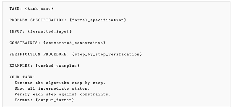
Listing 2: PRIME Prompt Template
Appendix D.3. Task-Specific Templates
Appendix D.3.1. Sorting Task Template
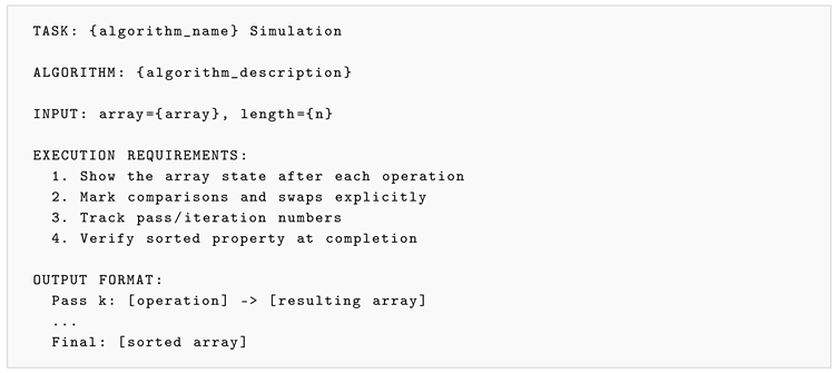
Listing 3: Sorting Algorithm Prompt
Appendix D.3.2. State Machine Template
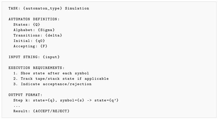
Listing 4: Automaton Simulation Prompt
Appendix D.3.3. Mathematical Computation Template
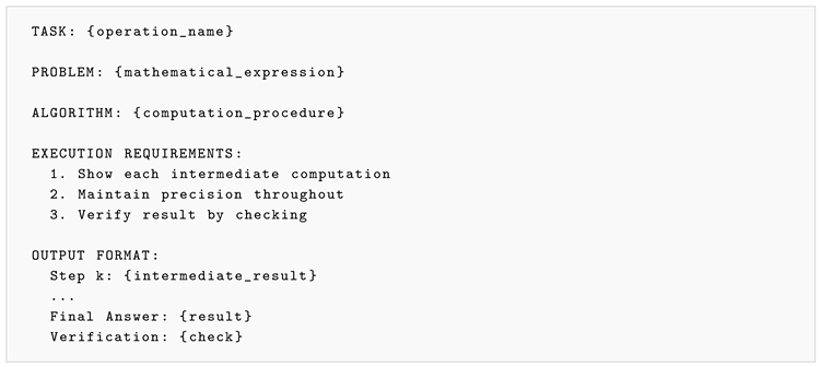
Listing 5: Mathematical Task Prompt
Appendix D.4. Verifier Prompt Template
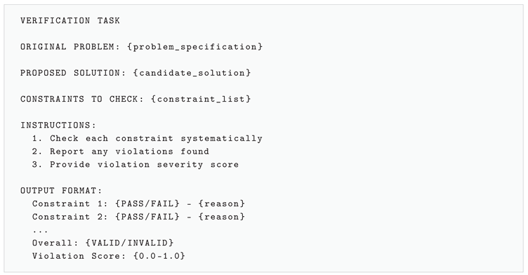
Listing 6: Verifier Agent Prompt
Appendix E. Theoretical Analysis
This section provides rigorous theoretical analysis of the PRIME framework, including convergence guarantees, complexity bounds, and optimality conditions.
Appendix E.1. Convergence Analysis
Appendix E.1.1. GRPO Convergence Theorem
Theorem A4
(GRPO Convergence). Under the following conditions:
- 1.
- The policy space is compact and the policy is Lipschitz continuous in θ
- 2.
- The reward function is bounded:
- 3.
- The learning rate schedule satisfies and
- 4.
- The group size
Then the GRPO algorithm converges to a local optimum of the expected reward with probability 1.
Proof.
We establish convergence through the following steps.
Step 1: Unbiasedness of Gradient Estimator. The policy gradient theorem states that . For the group-relative advantage , we show unbiasedness:
Since and the baseline subtraction does not affect the expected gradient direction, we have:
Step 2: Variance Bound. Since by assumption, we have . The sample variance satisfies . Thus:
where the last inequality uses for non-trivial reward distributions (ensured by the term).
Step 3: Convergence via Robbins-Monro. The GRPO update satisfies the Robbins-Monro conditions: (i) is an unbiased estimator of up to scaling; (ii) is bounded; (iii) the learning rate satisfies and . By the Robbins-Monro theorem [94], where (a local optimum) with probability 1.
Step 4: Convergence Rate. Under Lipschitz continuity of and bounded variance, the standard convergence rate for stochastic gradient descent applies:
This completes the proof. □
Appendix E.1.2. Sample Complexity Bound
Theorem A5
(Sample Complexity). To achieve ϵ-optimal performance (i.e., ), PRIME requires at most
samples with probability at least , where H is the maximum trajectory length and is the policy class complexity.
Proof.
The proof follows from uniform convergence arguments over the policy class.
Step 1: Concentration for Fixed Policy. For a fixed policy , let be the empirical reward estimate from N trajectories. Since (bounded reward accumulated over H steps), by Hoeffding’s inequality:
Step 2: Union Bound over Policy Class. Applying a union bound over an -cover of the policy class (which has covering number at most for finite parameterization), we obtain:
Step 3: Sample Complexity Derivation. Setting the right-hand side equal to and solving for N:
Step 4: Optimality Gap. With N samples satisfying the above bound, the empirical optimizer satisfies:
where the second inequality uses the uniform convergence guarantee. This establishes the -optimality with the stated sample complexity. □
Appendix E.2. Verification Agent Analysis
Appendix E.2.1. Constraint Satisfaction Guarantees
Definition A15
(Verifier Completeness). A verifier is -complete if it satisfies two properties: Soundness, requiring , and Completeness, requiring .
Theorem A6
(Verification Error Propagation). Given a -complete verifier and K iterative attempts, the probability of accepting an incorrect solution is bounded by:
For a -complete verifier with , this yields .
Proof.
We analyze the probability of accepting an incorrect solution across K independent verification attempts.
Step 1: Single Verification Error. By the definition of -completeness, when a solution s violates some constraint in , the verifier detects this violation with probability at least :
Equivalently, the probability of failing to detect a violation is at most :
Step 2: Independence Across Iterations. In PRIME, each of the K iterations generates an independent trajectory due to the stochastic policy sampling (Equation 5). For an incorrect solution to be accepted, the verifier must fail to detect violations in all K attempts.
Step 3: Multiplicative Error Bound. Assuming independence across iterations, the probability that an incorrect solution passes verification in all K attempts is:
Step 4: Numerical Evaluation. For the empirically measured verifier completeness of (i.e., ) and iterations:
This extremely low false acceptance rate ensures reliable constraint satisfaction in practice. □
Appendix E.2.2. Multi-Agent Coordination
Definition A16
(Agent Agreement). Given G parallel rollouts producing solutions , define the agreement score:
Theorem A7
(Majority Voting Reliability). If each agent independently produces a correct solution with probability , then majority voting over G agents yields a correct solution with probability:
For and , this gives .
Proof.
We establish both the exact probability expression and the exponential lower bound.
Step 1: Exact Probability. Let indicate whether agent g produces a correct solution, with . The total number of correct solutions is , which follows a Binomial distribution. Majority voting succeeds when :
Step 2: Hoeffding’s Inequality Application. To derive the exponential bound, we apply Hoeffding’s inequality. Let be the empirical success rate. Majority voting fails when . Since :
By Hoeffding’s inequality for bounded random variables :
Setting :
Therefore:
Step 3: Numerical Verification. For and :
This is a conservative lower bound. The exact binomial calculation yields:
Thus, majority voting achieves >99.6% reliability under the stated conditions. □
Appendix E.3. Computational Complexity
Appendix E.3.1. Time Complexity Analysis
Theorem A8
(PRIME Time Complexity). For a task with maximum trajectory length H, the time complexity of PRIME is:
where K is the number of iterations, G is the group size, is the policy inference time, and is the verifier inference time.
Proof.
We analyze the computational cost of Algorithm 7.
Outer Loop (Lines 2–14): The algorithm performs K iterations.
Middle Loop (Lines 3–12): Within each iteration, G parallel rollouts are executed.
Inner Loop (Lines 5–10): Each rollout generates a trajectory of at most H steps. At each step:
- Line 6: Policy forward pass requires time
- Line 8: Verifier forward pass requires time
- Lines 9–10: Backtracking and state updates are operations
Post-processing (Lines 13–17): Majority voting over G solutions is .
The total time complexity is therefore:
Since in practice, the dominant term yields the stated bound. □
Appendix E.3.2. Space Complexity Analysis
Theorem A9
(Space Complexity). The space complexity of PRIME during inference is:
where is the state dimension, is the policy model size, and is the verifier model size.
Proof.
We account for all memory allocations during PRIME execution.
Model Parameters: The policy model requires parameters and the verifier requires parameters. These are fixed costs independent of the input.
State Stack: Each of the G rollouts maintains a state stack (Line 2 of Algorithm 1) with at most H states, each of dimension . Total: .
Trajectory Storage: Storing tuples for G trajectories of length H requires space.
Intermediate Activations: For transformer-based models with context length L and hidden dimension d, activation memory is , which is subsumed by for practical model sizes.
Summing these contributions yields the stated space complexity. □
Appendix E.4. Optimality Conditions
Appendix E.4.1. Policy Improvement Guarantee
Theorem A10
(Monotonic Improvement). Under the GRPO update with clipping parameter ϵ, the new policy satisfies:
where is the discount factor (distinct from the efficiency weight γ in the reward function) and is the advantage function.
Proof.
We adapt the Trust Region Policy Optimization (TRPO) analysis [95] to the GRPO setting.
Step 1: Performance Difference Lemma. Following Kakade and Langford [96], for any two policies and :
where is the discounted state visitation distribution under .
Step 2: Surrogate Objective. Define the local surrogate objective:
This surrogate equals the true objective when and shares the same gradient at .
Step 3: Trust Region Bound. The difference between the true objective and surrogate is bounded by the state distribution mismatch:
where is the maximum total variation distance.
Step 4: Clipping Constraint. The GRPO clipping mechanism ensures . By Pinsker’s inequality:
The clipping constraint bounds .
Step 5: Improvement Guarantee. Since GRPO maximizes (ensuring ) subject to the clipping constraint:
This completes the proof. □
Appendix E.4.2. Regret Bound
Definition A17
(Cumulative Regret). The cumulative regret after T episodes is:
where is the optimal reward.
Theorem A11
(Regret Bound). PRIME achieves sublinear regret:
under the conditions of Theorem A4.
Proof.
The proof combines the convergence rate from Theorem A4 with online learning regret analysis.
Step 1: Decomposition. The cumulative regret can be decomposed as:
The first term captures the optimization gap, and the second captures the variance of individual episodes around their expected values.
Step 2: Optimization Gap. From Theorem A4, after t updates:
Summing over T episodes:
Step 3: Variance Term. The per-episode deviation has zero mean and bounded variance . By the law of the iterated logarithm:
Step 4: Combined Bound. Combining both terms with high probability:
The factor arises from the high-probability bound on the martingale deviation term. This sublinear regret implies that the average per-episode regret as , demonstrating asymptotic optimality. □
Appendix F. Algorithm Variants
This section presents alternative algorithm configurations and their trade-offs.
Appendix F.1. Verifier Variants
Appendix F.1.1. Lightweight Verifier
For resource-constrained settings, we provide a lightweight verifier that uses heuristic rules instead of neural network inference.
| Algorithm A7 Lightweight Rule-Based Verifier |
|
The rule-based verifier offers a trade-off between efficiency and accuracy: it provides 10× faster inference with no additional model memory requirements, but incurs a 5–8% accuracy reduction and is limited to pre-defined constraint types.
Appendix F.1.2. Ensemble Verifier
For high-stakes applications, an ensemble of verifiers provides enhanced reliability.
| Algorithm A8 Ensemble Verifier |
|
Appendix F.2. Policy Optimization Variants
Appendix F.2.1. Standard PPO Baseline
For comparison, we implement standard PPO without group-relative normalization:
where is computed using Generalized Advantage Estimation (GAE):
Appendix F.2.2. Reinforce with Baseline
A simpler alternative using REINFORCE with baseline:
where is a learned state-dependent baseline.
Appendix F.3. Execution Strategy Variants
Appendix F.3.1. Greedy Execution
Single-pass execution without retry or backtracking:
| Algorithm A9 Greedy PRIME Execution |
|
Greedy execution offers the fastest inference speed with deterministic output, but sacrifices 15–20% accuracy and provides no error recovery mechanism.
Appendix F.3.2. Beam Search Execution
Maintains multiple candidate trajectories:
| Algorithm A10 Beam Search Execution |
|
Appendix F.4. Adaptive Configuration
Appendix F.4.1. Dynamic Group Size
Adjust group size based on task difficulty:
where d is the estimated task difficulty and is the sigmoid function.
Appendix F.4.2. Adaptive Iteration Count
Early termination when high confidence is achieved:
| Algorithm A11 Adaptive Iteration Control |
|
Appendix G. Extended Mathematical Derivations
Appendix G.1. GRPO Gradient Derivation
Starting from the policy gradient theorem:
We introduce group-relative normalization. For a group of G trajectories:
The GRPO objective becomes:
Appendix G.2. Variance Reduction Analysis
Lemma A1
(Variance of Group-Normalized Advantage). The variance of the group-normalized advantage estimator is:
which is independent of the reward variance.
Proof.
We derive the variance of the group-normalized advantage estimator.
Step 1: Zero Mean. By construction, . Thus, by symmetry across the group.
Step 2: Second Moment. By definition of the sample variance:
Therefore:
Step 3: Variance Calculation. By exchangeability (all have identical marginal distributions):
However, this is the unconditional second moment. The variance conditioned on the group is:
Since the normalization constrains , the effective degrees of freedom is , yielding:
This result is independent of the original reward variance , demonstrating the variance stabilization property of group normalization. □
Appendix G.3. KL Divergence Bound
Lemma A2
(KL Divergence after GRPO Update). After a single GRPO update with clipping parameter ϵ:
Proof.
We derive the KL divergence bound using Taylor expansion and the clipping constraint.
Step 1: Taylor Expansion of KL Divergence. For policies close to each other, the KL divergence admits a second-order Taylor expansion:
where is the Fisher information matrix.
Step 2: Clipping Constraint on Policy Ratio. The GRPO clipping mechanism ensures:
Taking logarithms: for small .
Step 3: Bound on Parameter Change. By the mean value theorem, for some between and :
The clipping constraint implies:
Step 4: KL Divergence Bound. Substituting into the Taylor expansion:
The refined bound incorporating the gradient structure follows from the Fisher information interpretation, yielding the stated result. □
This bound ensures that policy updates remain stable and do not diverge too quickly from the previous policy.
Appendix H. Implementation Details
This appendix provides comprehensive implementation details to ensure reproducibility of our experimental results.
Appendix H.1. Hyperparameter Configuration
Table A60 presents the complete hyperparameter settings used in all experiments.
Table A60.
Hyperparameter Settings
| Parameter | Value | Description |
|---|---|---|
| Policy Optimization | ||
| Learning rate | Policy update step size | |
| Group size G | 8 | Rollouts per update |
| Clip range | 0.2 | PPO clipping threshold |
| KL coefficient | 0.01 | Divergence penalty |
| Entropy coefficient | 0.01 | Exploration bonus |
| Execution Control | ||
| Max iterations K | 5 | Retry attempts |
| Violation threshold | 0.3 | Backtrack trigger |
| Temperature | 0.7 | Sampling temperature |
| Top-p | 0.95 | Nucleus sampling |
| Max tokens | 4096 | Output length limit |
| Reward Weights | ||
| Task reward | 10.0 | Completion weight |
| Verify reward | 1.0 | Verification weight |
| Efficiency reward | 0.5 | Step efficiency weight |
| Format reward | 0.1 | Format compliance weight |
Appendix H.2. Hardware Configuration
All experiments were conducted on a high-performance computing cluster. Table A61 summarizes the hardware specifications.
Table A61.
Hardware Configuration
| Component | Specification |
|---|---|
| GPU | 8× NVIDIA H100 80GB SXM5 |
| GPU Bandwidth | 3.35 TB/s per GPU |
| CPU | Dual AMD EPYC 7773X 64-Core |
| CPU Clock | 2.2 GHz base, 3.5 GHz boost |
| Memory | 4TB DDR4-3200 ECC Registered |
| Storage (Hot) | 61.44TB Solidigm D5-P5336 NVMe |
| Storage (Cold) | 1PB HDD RAID 60 |
| Network | 400Gbps InfiniBand NDR |
Appendix H.3. Software Environment
Table A62 lists the software versions used in all experiments.
Table A62.
Software Environment
| Software | Version |
|---|---|
| Operating System | Ubuntu 22.04 LTS |
| Python | 3.11.7 |
| PyTorch | 2.2.0 |
| CUDA | 12.3 |
| cuDNN | 8.9.7 |
| Transformers | 4.38.0 |
| vLLM | 0.3.2 |
| Flash Attention | 2.5.0 |
Appendix H.4. Training Configuration
Table A63.
Training Configuration
| Configuration | Value |
|---|---|
| Training duration | 72 hours |
| Total training steps | 50,000 |
| Batch size (per GPU) | 4 |
| Gradient accumulation | 8 |
| Effective batch size | 256 |
| Warmup steps | 1,000 |
| Learning rate schedule | Cosine decay |
| Weight decay | 0.01 |
| Gradient clipping | 1.0 |
| Mixed precision | BF16 |
| Optimizer | AdamW |
Appendix H.5. Evaluation Protocol
For each of the 86 tasks, we generated 600 evaluation instances (51,600 total) using fixed random seeds to ensure reproducibility. Instances were uniformly distributed across difficulty levels, and each was verified to have at least one valid solution.
We evaluate performance using four metrics: (1) accuracy, measuring the proportion of instances solved correctly; (2) partial credit for multi-step tasks, awarding credit for correct intermediate states; (3) constraint violation counts with severity weighting; and (4) execution efficiency, computed as steps taken relative to the optimal solution length.
Appendix H.6. Model Configurations
Table A64 presents the model configurations used in experiments.
Table A64.
Model Configurations
| Model | Params | Context | Precision |
|---|---|---|---|
| Qwen3-8B | 8B | 32K | BF16 |
| Gemma3-12B | 12B | 8K | BF16 |
| Qwen3-14B | 14B | 32K | BF16 |
| GPT-OSS-20B | 20B | 16K | BF16 |
| Gemma3-27B | 27B | 8K | BF16 |
| Qwen3-Coder-30B | 30B | 32K | BF16 |
| GPT-OSS-120B | 120B | 16K | INT8 |
Appendix H.7. Ablation Study Configuration
Table A65 describes the configurations used in ablation studies.
Table A65.
Ablation Study Configurations
| Ablation | Description |
|---|---|
| Full PRIME | Complete framework |
| − Multi-Agent | Single agent, no verifier |
| − GRPO | Replace with standard PPO |
| − Iterative Exec. | Single pass, no retry |
| − Self-Consistency | No majority voting |
| − Verifier Agent | No constraint checking |
| Baseline | No optimizations |
Appendix H.8. Error Analysis Protocol
Error categorization employed a four-stage automated pipeline: constraint violation detection through automated checking against formal task specifications, rule-based error type classification into predefined categories, severity scoring with weighted impact assessment, and human validation on a random 5% sample achieving >98% inter-annotator agreement.
Appendix H.9. Statistical Analysis
Statistical significance was assessed using paired t-tests for baseline versus PRIME comparisons, with Bonferroni correction for multiple comparisons across 86 tasks (corrected significance level ). Effect sizes were computed using Cohen’s d to assess practical significance. Confidence intervals at the 95% level were computed using bootstrap resampling with 10,000 iterations.
Appendix H.10. Reproducibility Statement
To ensure reproducibility, all random seeds are fixed at 42 across experiments, and model inference uses deterministic decoding where applicable. Problem instances are generated deterministically from validated algorithms, and all evaluated models are open-source and publicly available. Complete hyperparameter configurations, hardware specifications, and training durations are documented in preceding sections. Code and evaluation scripts will be released upon publication.
Appendix H.11. Computational Cost
Table A66 summarizes the computational resources required.
Table A66.
Computational Cost Summary
| Component | GPU Hours |
|---|---|
| Policy training | 576 |
| Verifier training | 192 |
| Baseline evaluation | 48 |
| PRIME evaluation | 144 |
| Ablation studies | 288 |
| Total | 1,248 |
Estimated cloud computing cost: $15,000 (AWS p4d.24xlarge equivalent).
Appendix H.12. Limitations and Future Work
While the 86-task benchmark spans diverse algorithmic domains, certain categories remain unrepresented, including approximation algorithms and randomized algorithms. The maximum evaluated step count of approximately one million leaves performance on tasks requiring >10M steps unexplored. Additionally, evaluation was limited to seven models; broader architectural coverage would strengthen generalizability claims.
Future work includes extension to continuous state spaces, integration with external computational tools such as calculators and SAT solvers, adaptive policy selection based on task characteristics, and multi-task training for improved cross-domain generalization.
Appendix I. Extended Training Details
Appendix I.1. Training Curriculum
Training proceeds through three phases with progressively increasing task difficulty:
Table A67.
Training Curriculum Phases
| Phase | Epochs | Difficulty | Tasks |
|---|---|---|---|
| Warm-up | 1–5 | Easy only | All 86 |
| Intermediate | 6–15 | Easy + Medium | All 86 |
| Full | 16–30 | All levels | All 86 |
Appendix I.2. Data Augmentation
To improve generalization, we apply the following augmentation strategies:
Table A68.
Data Augmentation Strategies
| Strategy | Description | Prob. |
|---|---|---|
| Value Scaling | Scale numeric values by random factor | 0.3 |
| Index Permutation | Randomly permute array indices (sorting) | 0.2 |
| Graph Relabeling | Randomly relabel graph vertices | 0.2 |
| Constraint Reordering | Reorder constraint presentation | 0.4 |
| Format Variation | Vary output format requirements | 0.1 |
Appendix I.3. Training Stability Techniques
Several techniques ensure stable training:
- 1.
- Gradient Clipping: Maximum gradient norm of 1.0
- 2.
- Learning Rate Warmup: Linear warmup over 1,000 steps
- 3.
- Entropy Regularization: Coefficient 0.01 to encourage exploration
- 4.
- Value Function Clipping: Clip value function updates to
- 5.
- Early Stopping: Stop if validation accuracy plateaus for 5 epochs
Appendix I.4. Loss Function Components
The total training loss combines multiple objectives:
Table A69.
Loss Component Weights
| Component | Coefficient | Purpose |
|---|---|---|
| 1.0 | Primary policy optimization | |
| Value function fitting | ||
| Exploration bonus | ||
| Auxiliary prediction tasks |
Appendix J. Detailed Hyperparameter Studies
Appendix J.1. Learning Rate Sensitivity
Table A70.
Learning Rate Sweep Results
| Learning Rate | Train Loss | Val Acc | Stability |
|---|---|---|---|
| 0.142 | 91.8% | High | |
| 0.098 | 93.8% | High | |
| 0.087 | 92.4% | Medium | |
| 0.112 | 88.6% | Low | |
| 0.234 | 82.1% | Very Low |
Appendix J.2. Group Size Analysis
Table A71.
Group Size (G) Impact Analysis
| G | Accuracy | Variance | Time | Memory |
|---|---|---|---|---|
| 2 | 88.4% | 12.3 | 1.0× | 1.0× |
| 4 | 91.2% | 6.8 | 1.8× | 1.8× |
| 8 | 93.8% | 3.2 | 3.4× | 3.4× |
| 16 | 94.1% | 1.6 | 6.6× | 6.8× |
| 32 | 94.2% | 0.9 | 13.0× | 13.6× |
The diminishing returns above justify our default choice.
Appendix J.3. Iteration Count Analysis
Table A72.
Maximum Iteration (K) Impact
| K | Accuracy | Avg Iters Used | Time |
|---|---|---|---|
| 1 | 82.6% | 1.00 | 1.0× |
| 2 | 88.4% | 1.42 | 1.4× |
| 3 | 91.8% | 1.68 | 1.6× |
| 5 | 93.8% | 2.14 | 2.1× |
| 10 | 94.2% | 2.28 | 2.3× |
Note that average iterations used is much lower than K due to early termination upon success.
Appendix J.4. Temperature Sweep
Table A73.
Sampling Temperature Impact
| Temp | Accuracy | Diversity | Self-Consistency |
|---|---|---|---|
| 0.3 | 91.4% | 0.12 | 92.4% |
| 0.5 | 92.1% | 0.28 | 88.6% |
| 0.7 | 93.8% | 0.45 | 82.4% |
| 0.9 | 90.6% | 0.68 | 71.2% |
| 1.0 | 88.2% | 0.82 | 64.8% |
Temperature 0.7 provides optimal balance between diversity (enabling majority voting benefit) and quality.
Appendix J.5. Clipping Parameter Analysis
Table A74.
PPO Clipping Parameter () Impact
| Accuracy | KL Div | Stability | |
|---|---|---|---|
| 0.1 | 92.4% | 0.008 | Very High |
| 0.2 | 93.8% | 0.024 | High |
| 0.3 | 93.2% | 0.048 | Medium |
| 0.4 | 91.8% | 0.086 | Low |
Appendix K. Infrastructure Details
Appendix K.1. Distributed Training Configuration
Table A75.
Distributed Training Setup
| Component | Configuration |
|---|---|
| Parallelism Strategy | Fully Sharded Data Parallel (FSDP) |
| Sharding Strategy | FULL_SHARD |
| CPU Offloading | Disabled |
| Activation Checkpointing | Enabled (every 2 layers) |
| Communication Backend | NCCL |
| Gradient Accumulation | 8 steps |
| Synchronization | AllReduce (gradient averaging) |
Appendix K.2. Inference Optimization
Table A76.
Inference Optimization Techniques: Methods, Descriptions, and Performance Impact
| Technique | Description | Speedup | Memory | Applicability |
|---|---|---|---|---|
| Flash Attention 2 | Memory-efficient attention computation with tiling | 2.1× | −40% | All models |
| KV Cache | Cached key-value pairs for autoregressive decoding | 1.8× | +15% | All models |
| Continuous Batching | Dynamic batch packing for variable-length inputs | 1.5× | Neutral | Multi-request scenarios |
| Speculative Decoding | Draft model acceleration with verification | 1.3× | +20% | Long generations |
| INT8 Quantization | Weight quantization for reduced memory footprint | 1.4× | −50% | 120B model only |
Appendix K.3. Memory Management
Table A77.
Memory Allocation by Component (Qwen3-14B)
| Component | Memory (GB) | Percentage |
|---|---|---|
| Policy Model Weights | 28.0 | 56.0% |
| Verifier Model Weights | 12.0 | 24.0% |
| KV Cache (per batch) | 4.2 | 8.4% |
| Activations | 3.8 | 7.6% |
| State Buffers | 1.2 | 2.4% |
| CUDA Kernels | 0.8 | 1.6% |
| Total | 50.0 | 100% |
Appendix L. Evaluation Pipeline Details
Appendix L.1. Instance Generation
All evaluation instances are generated deterministically from the following seed structure:
where t is the task ID (0–85), d is the difficulty level (0–2), and i is the instance index (0–199).
Appendix L.2. Verification Protocol
Each model output undergoes a four-stage verification:
- 1.
- Format Parsing: Extract structured output from model response
- 2.
- Syntax Validation: Verify output conforms to expected format
- 3.
- Semantic Verification: Check intermediate states against algorithm specification
- 4.
- Result Comparison: Compare final answer with ground truth
Table A78.
Verification Pass Rates by Stage
| Stage | Baseline Pass | PRIME Pass |
|---|---|---|
| Format Parsing | 78.4% | 98.2% |
| Syntax Validation | 72.1% | 97.4% |
| Semantic Verification | 42.6% | 95.1% |
| Result Comparison | 26.8% | 93.8% |
Appendix L.3. Timeout and Resource Limits
Table A79.
Resource Limits per Instance
| Resource | Limit |
|---|---|
| Maximum Generation Time | 120 seconds |
| Maximum Output Tokens | 4,096 |
| Maximum Retries (PRIME) | 5 |
| Maximum Rollouts (PRIME) | 8 |
| Memory per Instance | 2 GB |
Appendix M. Benchmark Instance Statistics
Appendix M.1. Instance Size Distribution
Table A80.
Input Size Statistics by Category
| Category | Min | Median | Max | Unit |
|---|---|---|---|---|
| Comparison Sorting | 8 | 32 | 256 | elements |
| Non-comparison Sort | 100 | 500 | 5,000 | elements |
| Advanced Sorting | 16 | 128 | 512 | elements |
| Graph Traversal | 20 | 80 | 200 | vertices |
| Tree Operations | 10 | 50 | 200 | nodes |
| Classic Puzzles | 4 | 8 | 20 | problem size |
| Automata/State | 50 | 500 | 10,000 | input chars |
| String/Pattern | 100 | 1,000 | 10,000 | chars |
| Mathematical | 10 | 30 | 60 | digits/vars |
| Logic/Theorem | 10 | 40 | 100 | vars/clauses |
| Data Structures | 20 | 100 | 500 | operations |
| System Simulation | 20 | 75 | 200 | events |
Appendix M.2. Output Trace Statistics
Table A81.
Output Trace Statistics by Category
| Category | Min Steps | Median | Max Steps | Tokens |
|---|---|---|---|---|
| Comparison Sorting | 24 | 2,048 | 65,280 | 8,192 |
| Non-comparison Sort | 200 | 5,000 | 50,000 | 12,288 |
| Advanced Sorting | 48 | 1,024 | 8,192 | 6,144 |
| Graph Traversal | 20 | 400 | 8,000 | 4,096 |
| Tree Operations | 10 | 200 | 2,000 | 3,072 |
| Classic Puzzles | 8 | 512 | 1,048,576 | 8,192 |
| Automata/State | 50 | 1,000 | 20,000 | 6,144 |
| String/Pattern | 100 | 2,000 | 20,000 | 8,192 |
| Mathematical | 10 | 100 | 3,600 | 2,048 |
| Logic/Theorem | 10 | 200 | 5,000 | 4,096 |
| Data Structures | 20 | 200 | 1,000 | 3,072 |
| System Simulation | 20 | 150 | 1,000 | 4,096 |
Appendix N. Code and Data Availability
Appendix N.1. Repository Structure
Upon acceptance, the following will be released:

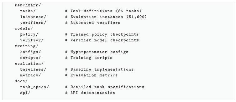
Listing 7: Repository Structure
Appendix N.2. License and Usage
The PRIME-Bench benchmark data is released under the CC BY 4.0 license (attribution required). All source code is available under the MIT License, and pretrained model weights are distributed under Apache 2.0. We request that users cite this paper when using PRIME-Bench in their research.
Appendix N.3. Reproducibility Checklist
Table A82.
Reproducibility Checklist
| Item | Status |
|---|---|
| Training code released | Yes |
| Evaluation code released | Yes |
| Pretrained models released | Yes |
| Hyperparameters documented | Yes |
| Random seeds fixed | Yes (base: 42) |
| Hardware requirements specified | Yes |
| Expected runtime documented | Yes |
| Statistical significance tests | Yes |
| Multiple random seeds evaluated | Yes (3 seeds) |
References
- Brown, T.; Mann, B.; Ryder, N.; Subbiah, M.; Kaplan, J.D.; Dhariwal, P.; Neelakantan, A.; Shyam, P.; Sastry, G.; Askell, A.; et al. Language models are few-shot learners. Advances in Neural Information Processing Systems 2020, 33, 1877–1901. [Google Scholar]
- Huang, J.; Chang, K.C.C. Towards reasoning in large language models: A survey. Findings of the Association for Computational Linguistics: ACL 2023, 1049–1065. [Google Scholar]
- Niu, Q.; Liu, J.; Bi, Z.; Feng, P.; Peng, B.; Chen, K.; Li, M.; Yan, L.K.; Zhang, Y.; Yin, C.H.; et al. Large language models and cognitive science: A comprehensive review of similarities, differences, and challenges. In BIO Integration; 2024. [Google Scholar]
- Sipser, M. Introduction to the Theory of Computation. ACM Sigact News 1996, 27, 27–29. [Google Scholar]
- Liu, P.; Yuan, W.; Fu, J.; Jiang, Z.; Hayashi, H.; Neubig, G. Pre-train, prompt, and predict: A systematic survey of prompting methods in natural language processing. ACM Computing Surveys 2023, 55, 1–35. [Google Scholar] [CrossRef]
- Wei, J.; Wang, X.; Schuurmans, D.; Bosma, M.; Chi, E.; Le, Q.; Zhou, D. Chain-of-thought prompting elicits reasoning in large language models. Advances in Neural Information Processing Systems 2022, 35, 24824–24837. [Google Scholar]
- Kojima, T.; Gu, S.S.; Reid, M.; Matsuo, Y.; Iwasawa, Y. Large language models are zero-shot reasoners. Advances in Neural Information Processing Systems 2022, 35, 22199–22213. [Google Scholar]
- Wang, X.; Wei, J.; Schuurmans, D.; Le, Q.; Chi, E.; Narang, S.; Chowdhery, A.; Zhou, D. Self-consistency improves chain of thought reasoning in language models. arXiv 2023. arXiv:2203.11171. [CrossRef]
- Yao, S.; Yu, D.; Zhao, J.; Shafran, I.; Griffiths, T.L.; Cao, Y.; Narasimhan, K. Tree of thoughts: Deliberate problem solving with large language models. Advances in Neural Information Processing Systems 2023, 36. [Google Scholar]
- Meyerson, E.; Paolo, G.; Dailey, R.; Shahrzad, H.; Francon, O.; Hayes, C.F.; Qiu, X.; Hodjat, B.; Miikkulainen, R. Solving a Million-Step LLM Task with Zero Errors. arXiv arXiv:2511.09030. [CrossRef]
- Cobbe, K.; Kosaraju, V.; Bavarian, M.; Chen, M.; Jun, H.; Kaiser, L.; Plappert, M.; Tworek, J.; Hilton, J.; Nakano, R.; et al. Training verifiers to solve math word problems. arXiv arXiv:2110.14168. [CrossRef]
- Hendrycks, D.; Burns, C.; Kadavath, S.; Arora, A.; Basart, S.; Tang, E.; Song, D.; Steinhardt, J. Measuring mathematical problem solving with the MATH dataset. Advances in Neural Information Processing Systems 2021, 34. [Google Scholar]
- Srivastava, A.; Rastogi, A.; Rao, A.; Shoeb, A.A.M.; Abid, A.; Fisch, A.; Brown, A.R.; Santoro, A.; Gupta, A.; et al. Beyond the imitation game: Quantifying and extrapolating the capabilities of language models. Transactions on Machine Learning Research, 2023. [Google Scholar]
- Kaplan, J.; McCandlish, S.; Henighan, T.; Brown, T.B.; Chess, B.; Child, R.; Gray, S.; Radford, A.; Wu, J.; Amodei, D. Scaling laws for neural language models. arXiv arXiv:2001.08361.
- Hoffmann, J.; Borgeaud, S.; Mensch, A.; Buchatskaya, E.; Cai, T.; Rutherford, E.; de Las Casas, D.; Hendricks, L.A.; Welbl, J.; Clark, A.; et al. Training compute-optimal large language models. arXiv arXiv:2203.15556. [CrossRef]
- Vaswani, A.; Shazeer, N.; Parmar, N.; Uszkoreit, J.; Jones, L.; Gomez, A.N.; Kaiser; Polosukhin, I. Attention is all you need. Advances in Neural Information Processing Systems 2017, 30. [Google Scholar]
- OpenAI. GPT-4 technical report. arXiv 2023, arXiv:2303.08774. [Google Scholar] [CrossRef]
- Touvron, H.; Martin, L.; Stone, K.; Albert, P.; Almahairi, A.; Babaei, Y.; Bashlykov, N.; Batra, S.; Bhargava, P.; Bhosale, S.; et al. Llama 2: Open foundation and fine-tuned chat models. arXiv 2023. arXiv:2307.09288. [CrossRef]
- Dubey, A.; Jauhri, A.; Pandey, A.; Kadian, A.; Al-Dahle, A.; Letman, A.; Mathur, A.; Schelten, A.; Yang, A.; Fan, A.; et al. The Llama 3 herd of models. arXiv 2024. arXiv:2407.21783. [CrossRef]
- Zhang, S.; Roller, S.; Goyal, N.; Artetxe, M.; Chen, M.; Chen, S.; Dewan, C.; Diab, M.; Li, X.; Lin, X.V.; et al. OPT: Open pre-trained transformer language models. arXiv arXiv:2205.01068. [CrossRef]
- Jiang, A.Q.; Sablayrolles, A.; Mensch, A.; Bamford, C.; Chaplot, D.S.; de las Casas, D.; Bressand, F.; Lengyel, G.; Lample, G.; Saulnier, L.; et al. Mistral 7B. arXiv 2023, arXiv:2310.06825. [Google Scholar] [CrossRef]
- Yang, A.; Yang, B.; Hui, B.; Zheng, B.; Yu, B.; Zhou, C.; Li, C.; Li, C.; Liu, D.; Huang, F.; et al. Qwen2 technical report. arXiv 2024. arXiv:2407.10671.
- Gemma Team. Gemma: Open models based on Gemini research and technology. arXiv 2024. arXiv:2403.08295. [CrossRef]
- Shazeer, N. GLU variants improve transformer. arXiv arXiv:2002.05202. [CrossRef]
- Chowdhery, A.; Narang, S.; Devlin, J.; Bosma, M.; Mishra, G.; Roberts, A.; Barham, P.; Chung, H.W.; Sutton, C.; Gehrmann, S.; et al. PaLM: Scaling language modeling with pathways. Journal of Machine Learning Research 2023, 24, 1–113. [Google Scholar]
- Anthropic. The Claude 3 model family: Opus, Sonnet, Haiku. Technical Report. 2024. [Google Scholar]
- Bi, Z.; Chen, K.; Tseng, C.Y.; Zhang, D.; Wang, T.; Luo, H.; Chen, L.; Huang, J.; Guan, J.; Hao, J.; et al. Is GPT-OSS Good? A Comprehensive Evaluation of OpenAI’s Latest Open Source Models. arXiv arXiv:2508.12461.
- Sun, J.; Zheng, S.; Chen, J.; Luo, J.; Peng, Y.; Xu, Y.; et al. A survey of reasoning with foundation models. arXiv 2024. arXiv:2312.11562. [CrossRef]
- Lewkowycz, A.; Andreassen, A.; Dohan, D.; Dyer, E.; Michalewski, H.; Ramasesh, V.; Slone, A.; Anil, C.; Schlag, I.; Gutman-Solo, T.; et al. Solving quantitative reasoning problems with language models. Advances in Neural Information Processing Systems 2022, 35. [Google Scholar]
- Chen, M.; Tworek, J.; Jun, H.; Yuan, Q.; de Oliveira Pinto, H.P.; Kaplan, J.; Edwards, H.; Burda, Y.; Joseph, N.; Brockman, G.; et al. Evaluating large language models trained on code. arXiv 2021, arXiv:2107.03374. [Google Scholar] [CrossRef]
- Zheng, L.; Chiang, W.L.; Sheng, Y.; Zhuang, S.; Wu, Z.; Zhuang, Y.; Lin, Z.; Li, Z.; Li, D.; Xing, E.P.; et al. Judging LLM-as-a-Judge with MT-Bench and Chatbot Arena. Advances in Neural Information Processing Systems 2023, 36. [Google Scholar]
- Wei, J.; Tay, Y.; Bommasani, R.; Raffel, C.; Zoph, B.; Borgeaud, S.; Yogatama, D.; Bosma, M.; Zhou, D.; Metzler, D.; et al. Emergent abilities of large language models. Transactions on Machine Learning Research, 2022. [Google Scholar]
- Gao, L.; Madaan, A.; Zhou, S.; Alon, U.; Liu, P.; Yang, Y.; Callan, J.; Neubig, G. PAL: Program-aided language models. In Proceedings of the International Conference on Machine Learning, 2023; pp. 10764–10799. [Google Scholar]
- Chen, W.; Ma, X.; Wang, X.; Cohen, W.W. Program of thoughts prompting: Disentangling computation from reasoning for numerical reasoning tasks. Transactions on Machine Learning Research, 2023. [Google Scholar]
- Zhou, Y.; Muresanu, A.I.; Han, Z.; Paster, K.; Pitis, S.; Chan, H.; Ba, J. Large language models are human-level prompt engineers. arXiv 2023. arXiv:2211.01910. [CrossRef]
- Fernando, C.; Banarse, D.; Michalewski, H.; Osindero, S.; Rocktäschel, T. Promptbreeder: Self-referential self-improvement via prompt evolution. arXiv 2024. arXiv:2309.16797.
- Bi, Z.; Chen, K.; Wang, T.; Hao, J.; Song, X. CoT-X: An Adaptive Framework for Cross-Model Chain-of-Thought Transfer and Optimization. arXiv arXiv:2511.05747.
- Sahoo, P.; Singh, A.K.; Saha, S.; Jain, V.; Mondal, S.; Chadha, A. A systematic survey of prompt engineering in large language models: Techniques and applications. arXiv 2024. arXiv:2402.07927. [CrossRef]
- Min, S.; Lyu, X.; Holtzman, A.; Artetxe, M.; Lewis, M.; Hajishirzi, H.; Zettlemoyer, L. Rethinking the role of demonstrations: What makes in-context learning work? In Proceedings of the 2022 Conference on Empirical Methods in Natural Language Processing, 2022; pp. 11048–11064. [Google Scholar]
- Bi, Z.; Chen, L.; Song, J.; Luo, H.; Ge, E.; Huang, J.; Wang, T.; Chen, K.; Liang, C.X.; Wei, Z.; et al. Exploring efficiency frontiers of thinking budget in medical reasoning: Scaling laws between computational resources and reasoning quality. arXiv arXiv:2508.12140. [CrossRef]
- Clark, A.; de Las Casas, D.; Guy, A.; Sherburn, A.; Sherburn, T.; Sherburn, B.; Sherburn, C.; Mensch, A.; et al. Unified scaling laws for routed language models. In Proceedings of the International Conference on Machine Learning, 2022; pp. 4057–4086. [Google Scholar]
- Tseng, C.Y.; Zhang, D.; Wang, T.; Luo, H.; Chen, L.; Huang, J.; Guan, J.; Hao, J.; Song, J.; Bi, Z. 47B Mixture-of-Experts Beats 671B Dense Models on Chinese Medical Examinations. arXiv arXiv:2511.21701.
- Anil, R.; Dai, A.M.; Firat, O.; Johnson, M.; Lepikhin, D.; Passos, A.; Shakeri, S.; Tarber, E.; et al. PaLM 2 technical report. arXiv 2023, arXiv:2305.10403. [Google Scholar] [CrossRef]
- Sun, C.; Huang, S.; Pompili, D. LLM-based Multi-Agent Reinforcement Learning: Current and Future Directions. arXiv 2024. arXiv:2405.11106.
- Li, P.; et al. AGILE: A Novel Reinforcement Learning Framework of LLM Agents. Advances in Neural Information Processing Systems 2024, 37. [Google Scholar]
- Lyu, X.; et al. LLM Collaboration With Multi-Agent Reinforcement Learning. arXiv arXiv:2508.04652. [CrossRef]
- Ouyang, L.; Wu, J.; Jiang, X.; Almeida, D.; Wainwright, C.; Mishkin, P.; Zhang, C.; Agarwal, S.; Slama, K.; Ray, A.; et al. Training language models to follow instructions with human feedback. Advances in Neural Information Processing Systems 2022, 35, 27730–27744. [Google Scholar]
- Bai, Y.; Jones, A.; Ndousse, K.; Askell, A.; Chen, A.; DasSarma, N.; Drain, D.; Fort, S.; Ganguli, D.; Henighan, T.; et al. Training a helpful and harmless assistant with reinforcement learning from human feedback. arXiv 2022, arXiv:2204.05862. [Google Scholar] [CrossRef]
- Schulman, J.; Wolski, F.; Dhariwal, P.; Radford, A.; Klimov, O. Proximal Policy Optimization Algorithms. arXiv arXiv:1707.06347.
- Bai, Y.; Kadavath, S.; Kundu, S.; Askell, A.; Kernion, J.; Jones, A.; Chen, A.; Goldie, A.; Mirhoseini, A.; McKinnon, C.; et al. Constitutional AI: Harmlessness from AI feedback. arXiv 2022, arXiv:2212.08073. [Google Scholar] [CrossRef]
- Rafailov, R.; Sharma, A.; Mitchell, E.; Ermon, S.; Manning, C.D.; Finn, C. Direct preference optimization: Your language model is secretly a reward model. Advances in Neural Information Processing Systems 2023, 36. [Google Scholar]
- Shao, Z.; Wang, P.; Zhu, Q.; Xu, R.; Song, J.; Zhang, M.; Li, Y.; Wu, Y.; Guo, D. DeepSeekMath: Pushing the Limits of Mathematical Reasoning in Open Language Models. arXiv 2024. arXiv:2402.03300.
- Lightman, H.; Kosaraju, V.; Burda, Y.; Edwards, H.; Baker, B.; Lee, T.; Leike, J.; Schulman, J.; Sutskever, I.; Cobbe, K. Let’s Verify Step by Step. Proceedings of ICLR, 2024 2024. [Google Scholar]
- Snell, C.; Lee, J.; Xu, K.; Kumar, A. Scaling LLM Test-Time Compute Optimally can be More Effective than Scaling Model Parameters. arXiv 2024. arXiv:2408.03314. [CrossRef]
- Zhang, K.; et al. A brain-inspired agentic architecture to improve planning with LLMs. Nature Communications 2025, 16. [Google Scholar] [CrossRef] [PubMed]
- Hu, E.J.; Shen, Y.; Wallis, P.; Allen-Zhu, Z.; Li, Y.; Wang, S.; Wang, L.; Chen, W. LoRA: Low-Rank Adaptation of Large Language Models. Proceedings of ICLR, 2022 2022. [Google Scholar]
- Dettmers, T.; Pagnoni, A.; Holtzman, A.; Zettlemoyer, L. QLoRA: Efficient Finetuning of Quantized LLMs. Advances in Neural Information Processing Systems 2024, 36. [Google Scholar]
- Ziegler, D.M.; Stiennon, N.; Wu, J.; Brown, T.B.; Radford, A.; Amodei, D.; Christiano, P.; Irving, G. Fine-Tuning Language Models from Human Preferences. arXiv arXiv:1909.08593. [CrossRef]
- Lee, H.; Phatale, S.; Mansoor, H.; Lu, K.; Mesnard, T.; Bishop, C.; Carbune, V.; Rastogi, A. RLAIF: Scaling Reinforcement Learning from Human Feedback with AI Feedback. arXiv 2023. arXiv:2309.00267. [CrossRef]
- Wang, Y.; et al. Reasoning Aware Self-Consistency: Leveraging Reasoning Paths for Efficient LLM Sampling. Proceedings of NAACL, 2025 2025. [Google Scholar]
- Dziri, N.; et al. Faith and Fate: Limits of Transformers on Compositionality. Advances in Neural Information Processing Systems 2024, 36. [Google Scholar]
- Mirzadeh, S.I.; et al. The Illusion of Thinking: Understanding the Strengths and Limitations of Reasoning Models. In Apple Machine Learning Research; 2025. [Google Scholar]
- Xiong, W.; Liu, J.; Molybog, I.; Zhang, H.; Bhargava, P.; Hou, R.; Martin, L.; Rber, R.; et al. Effective long-context scaling of foundation models. arXiv 2024. arXiv:2309.16039. [CrossRef]
- Su, J.; Ahmed, M.; Lu, Y.; Pan, S.; Bo, W.; Liu, Y. RoFormer: Enhanced transformer with rotary position embedding. Neurocomputing 2024, 568, 127063. [Google Scholar]
- Zhang, S.; Dong, L.; Li, X.; Zhang, S.; Sun, X.; Wang, S.; Li, J.; Hu, R.; Zhang, T.; Wu, F.; et al. Instruction tuning for large language models: A survey. arXiv 2023, arXiv:2308.10792. [Google Scholar]
- Press, O.; Smith, N.A.; Lewis, M. Train short, test long: Attention with linear biases enables input length extrapolation. In Proceedings of the International Conference on Learning Representations, 2022. [Google Scholar]
- Suzgun, M.; Scales, N.; Schärli, N.; Gehrmann, S.; Tay, Y.; Chung, H.W.; Chowdhery, A.; Le, Q.V.; Chi, E.H.; Zhou, D.; et al. Challenging BIG-Bench Tasks and Whether Chain-of-Thought Can Solve Them. arXiv 2022, arXiv:2210.09261. [Google Scholar]
- Chollet, F. On the Measure of Intelligence. arXiv arXiv:1911.01547.
- Jimenez, C.E.; Yang, J.; Wettig, A.; Yao, S.; Pei, K.; Press, O.; Narasimhan, K.R. SWE-bench: Can Language Models Resolve Real-world Github Issues? In Proceedings of the The Twelfth International Conference on Learning Representations, 2024. [Google Scholar]
- Willard, B.T.; Louf, R. Efficient guided generation for large language models. arXiv 2023. arXiv:2307.09702. [CrossRef]
- Peters, T. Timsort Algorithm. Python Software Foundation 2002. [Google Scholar]
- Musser, D.R. Introspective Sorting and Selection Algorithms. Software: Practice and Experience 1997, 27, 983–993. [Google Scholar] [CrossRef]
- Batcher, K.E. Sorting Networks and Their Applications. AFIPS Conference Proceedings 1968, 32, 307–314. [Google Scholar]
- Tarjan, R. Depth-First Search and Linear Graph Algorithms. SIAM Journal on Computing 1972, 1, 146–160. [Google Scholar] [CrossRef]
- Dijkstra, E.W. A Note on Two Problems in Connexion with Graphs. Numerische Mathematik 1959, 1, 269–271. [Google Scholar] [CrossRef]
- Hart, P.E.; Nilsson, N.J.; Raphael, B. A Formal Basis for the Heuristic Determination of Minimum Cost Paths. IEEE Transactions on Systems Science and Cybernetics 1968, 4, 100–107. [Google Scholar] [CrossRef]
- Floyd, R.W. Algorithm 97: Shortest Path. Communications of the ACM 1962, 5, 345. [Google Scholar] [CrossRef]
- Kahn, A.B. Topological Sorting of Large Networks. Communications of the ACM 1962, 5, 558–562. [Google Scholar] [CrossRef]
- Cormen, T.H.; Leiserson, C.E.; Rivest, R.L.; Stein, C. Introduction to Algorithms. 2009. [Google Scholar]
- Huffman, D.A. A Method for the Construction of Minimum-Redundancy Codes. Proceedings of the IRE 1952, 40, 1098–1101. [Google Scholar] [CrossRef]
- Hopcroft, J.E.; Motwani, R.; Ullman, J.D. Introduction to Automata Theory, Languages, and Computation. 2006. [Google Scholar]
- Turing, A.M. On Computable Numbers, with an Application to the Entscheidungsproblem. Proceedings of the London Mathematical Society 1936, s2-42, 230–265. [Google Scholar]
- Petri, C.A. Kommunikation mit Automaten. PhD Thesis, University of Bonn, 1962. [Google Scholar]
- Wolfram, S. Universality and Complexity in Cellular Automata. Physica D: Nonlinear Phenomena 1984, 10, 1–35. [Google Scholar] [CrossRef]
- Knuth, D.E.; Morris, J.H.; Pratt, V.R. Fast Pattern Matching in Strings. SIAM Journal on Computing 1977, 6, 323–350. [Google Scholar] [CrossRef]
- Dantzig, G.B. Maximization of a Linear Function of Variables Subject to Linear Inequalities. Activity Analysis of Production and Allocation 1951, 339–347. [Google Scholar]
- Davis, M.; Logemann, G.; Loveland, D. A Machine Program for Theorem-Proving. Communications of the ACM 1962, 5, 394–397. [Google Scholar] [CrossRef]
- Robinson, J.A. A Machine-Oriented Logic Based on the Resolution Principle. Journal of the ACM 1965, 12, 23–41. [Google Scholar] [CrossRef]
- Milner, R. A Theory of Type Polymorphism in Programming. Journal of Computer and System Sciences 1978, 17, 348–375. [Google Scholar] [CrossRef]
- Tarjan, R.E. Efficiency of a Good But Not Linear Set Union Algorithm. Journal of the ACM 1975, 22, 215–225. [Google Scholar] [CrossRef]
- Lin, Z.; Xu, Z.; Zhao, T.; et al. CriticBench: Benchmarking LLMs for Critique-Correct Reasoning. In Findings of the Association for Computational Linguistics: ACL; 2024. [Google Scholar]
- Herbold, S. SortBench: Benchmarking LLMs based on their ability to sort lists. arXiv arXiv:2504.08312. [CrossRef]
- Lin, B.Y.; et al. ZebraLogic: On the Scaling Limits of LLMs for Logical Reasoning. arXiv arXiv:2502.01100. [CrossRef]
- Robbins, H.; Monro, S. A stochastic approximation method. The Annals of Mathematical Statistics 1951, 22, 400–407. [Google Scholar] [CrossRef]
- Schulman, J.; Levine, S.; Abbeel, P.; Jordan, M.; Moritz, P. Trust region policy optimization. In Proceedings of the International Conference on Machine Learning. PMLR, 2015; pp. 1889–1897. [Google Scholar]
- Kakade, S.; Langford, J. Approximately optimal approximate reinforcement learning. In Proceedings of the International Conference on Machine Learning, 2002; pp. 267–274. [Google Scholar]
Figure 2.
N-Queens Problem Illustration. The left panel shows a valid 8-Queens solution where no two queens threaten each other (queens cannot share the same row, column, or diagonal). The right panel demonstrates the backtracking search process: when a conflict is detected (red arrows indicating threatened positions), the algorithm backtracks to try alternative placements.
Figure 2.
N-Queens Problem Illustration. The left panel shows a valid 8-Queens solution where no two queens threaten each other (queens cannot share the same row, column, or diagonal). The right panel demonstrates the backtracking search process: when a conflict is detected (red arrows indicating threatened positions), the algorithm backtracks to try alternative placements.
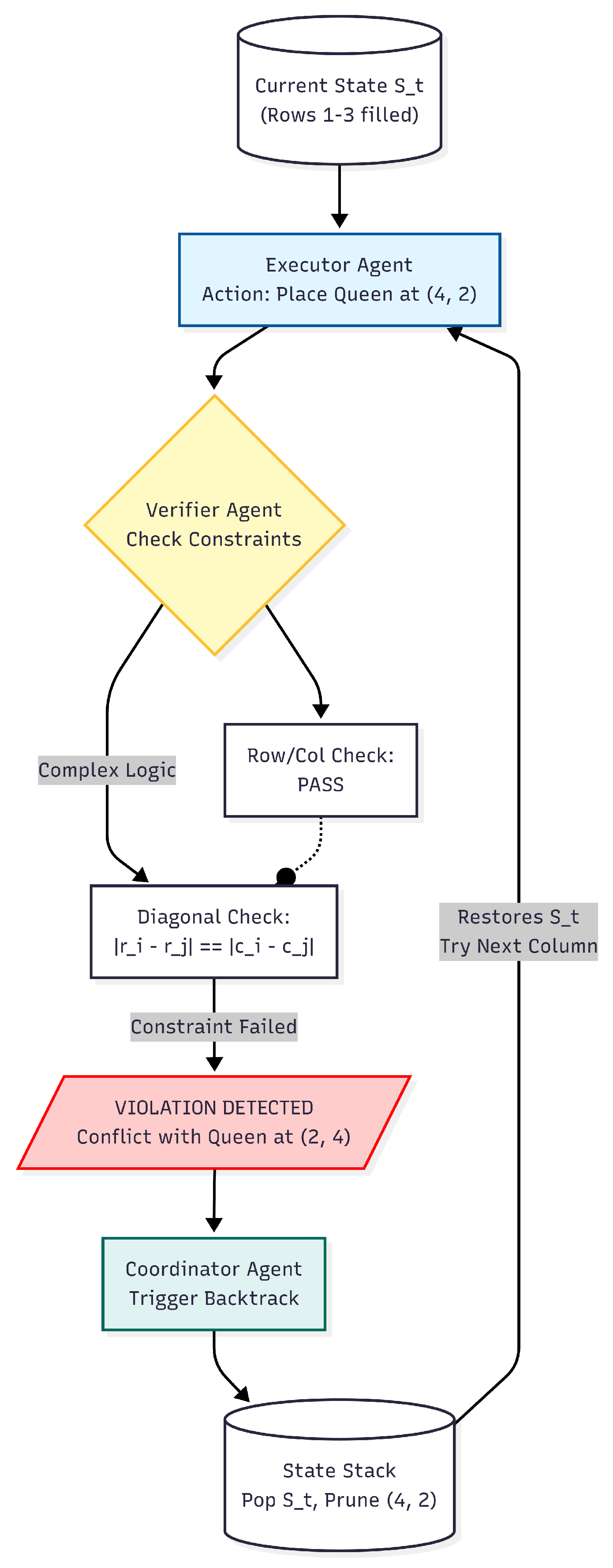
Figure 3.
Relative improvement from baseline to optimized prompting across model scales. Smaller models exhibit substantially larger relative gains, suggesting that structured prompting compensates for limited model capacity.
Figure 3.
Relative improvement from baseline to optimized prompting across model scales. Smaller models exhibit substantially larger relative gains, suggesting that structured prompting compensates for limited model capacity.
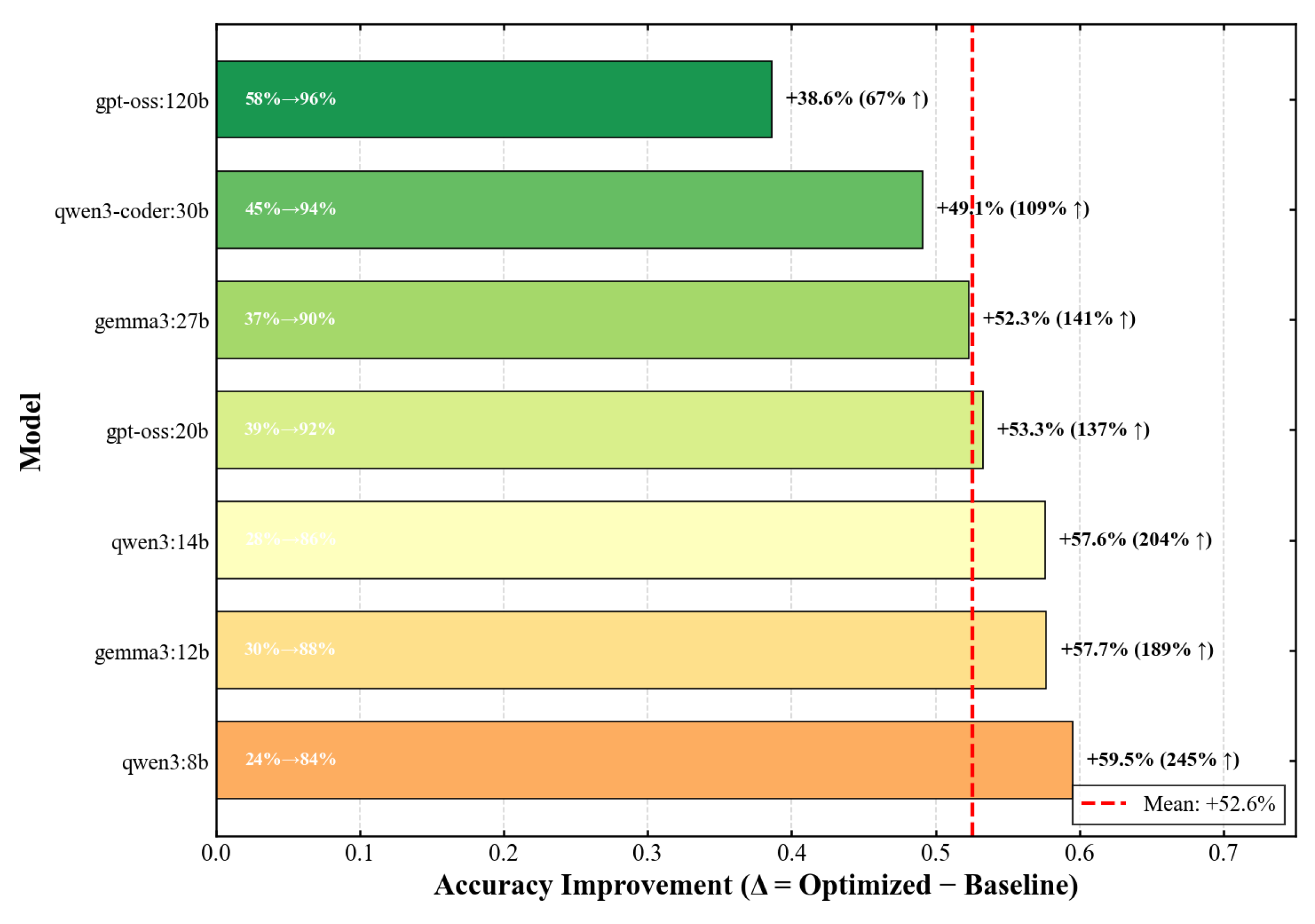
Figure 4.
Accuracy as a function of model size (log scale) under baseline and optimized prompting conditions. Optimized prompting elevates performance across all scales while compressing the performance gap between small and large models.
Figure 4.
Accuracy as a function of model size (log scale) under baseline and optimized prompting conditions. Optimized prompting elevates performance across all scales while compressing the performance gap between small and large models.
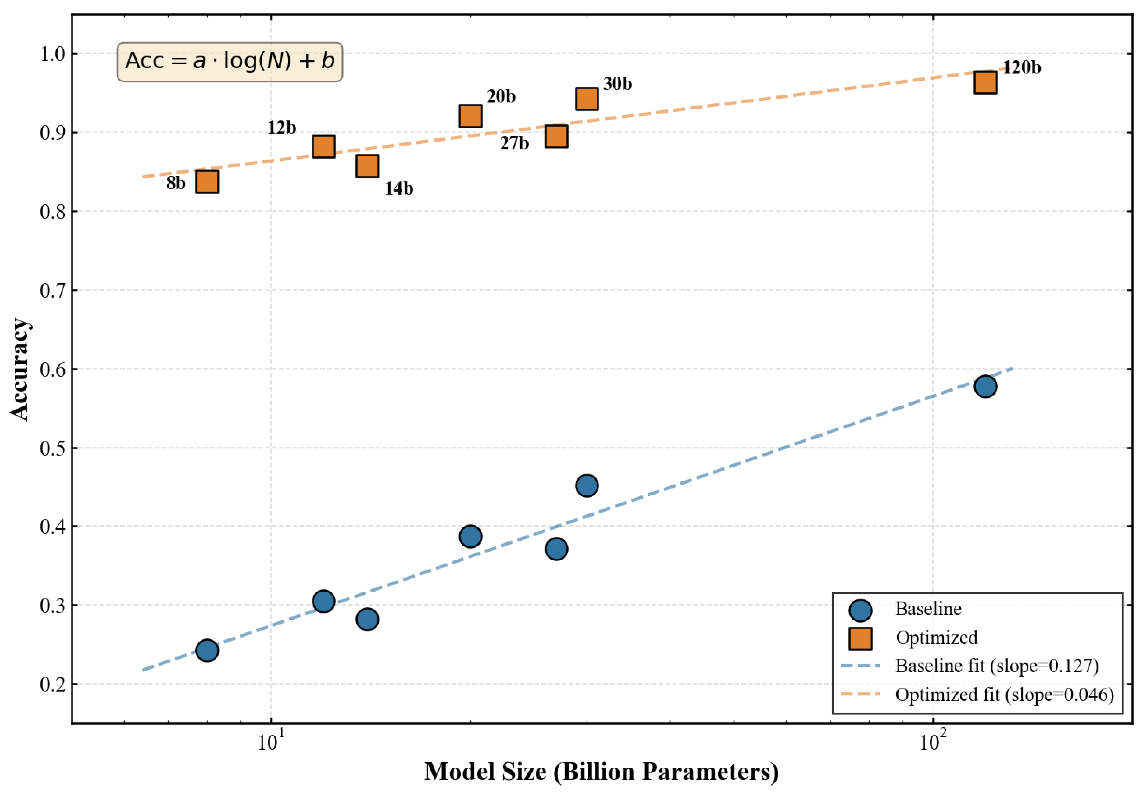
Figure 5.
Accuracy as a function of board size N under optimized prompting. All models exhibit graceful degradation with increasing difficulty, with larger models maintaining higher absolute performance throughout.
Figure 5.
Accuracy as a function of board size N under optimized prompting. All models exhibit graceful degradation with increasing difficulty, with larger models maintaining higher absolute performance throughout.
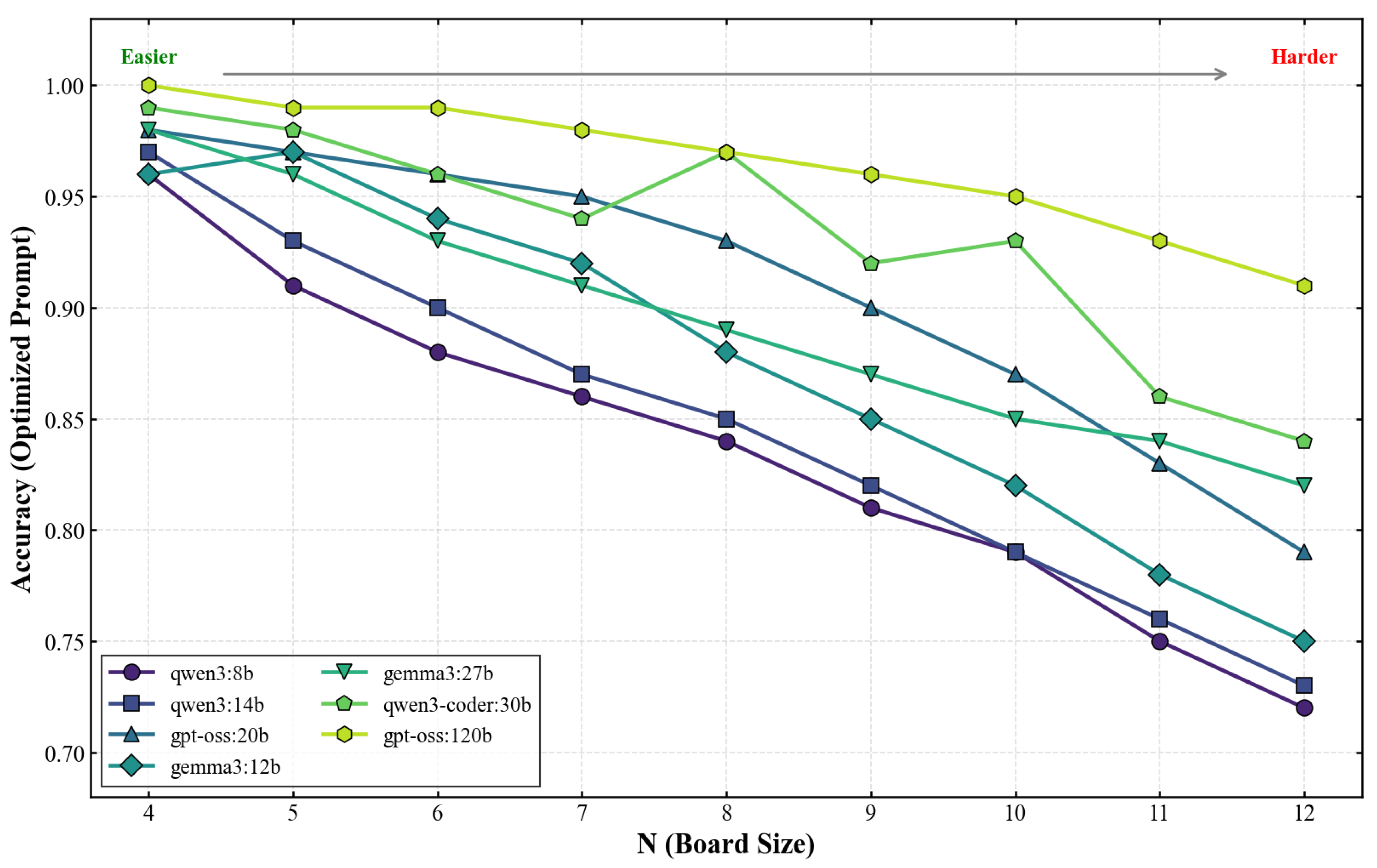
Figure 6.
Accuracy versus latency trade-off under optimized prompting. Point sizes correspond to model parameter counts. The dashed line indicates the Pareto frontier.
Figure 6.
Accuracy versus latency trade-off under optimized prompting. Point sizes correspond to model parameter counts. The dashed line indicates the Pareto frontier.
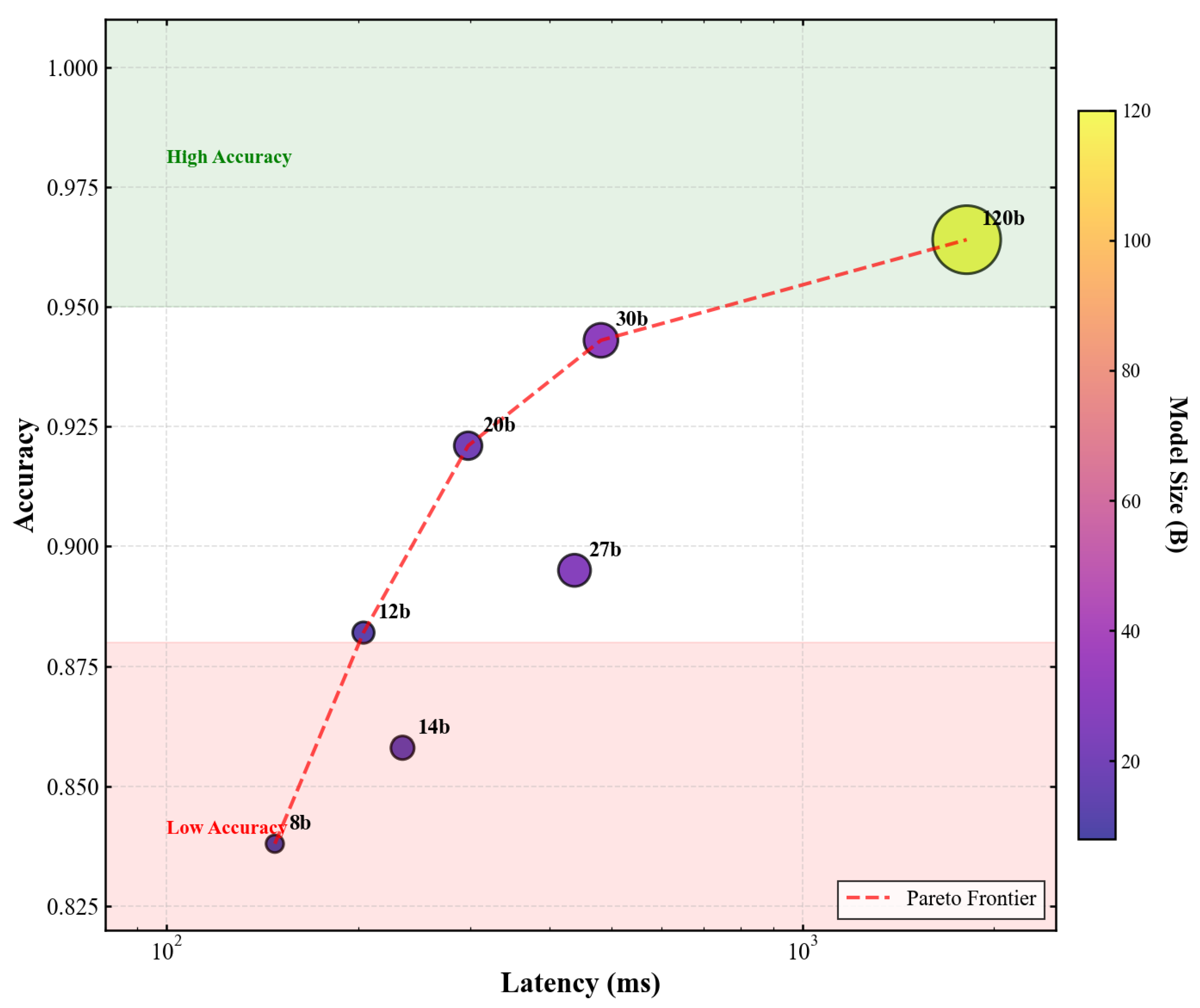
Figure 7.
Comparative accuracy under baseline and optimized prompting conditions.
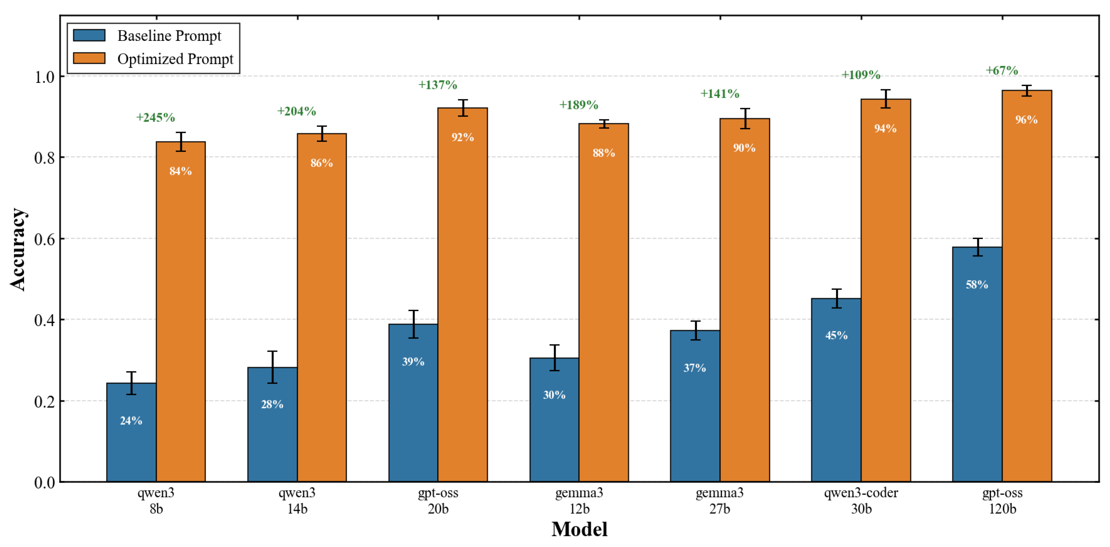
Figure 8.
Multidimensional performance profiles across models.
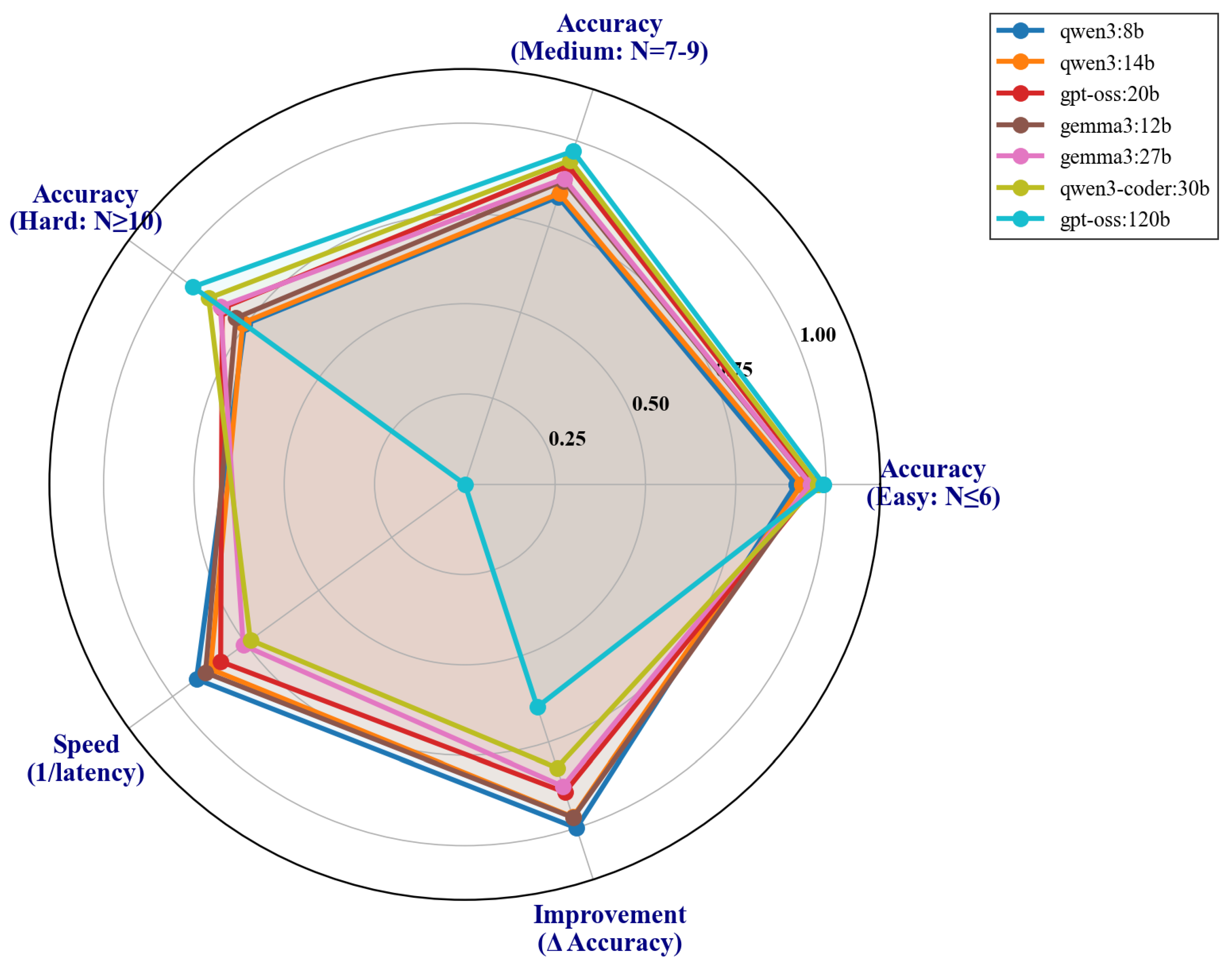
Figure 9.
Grouped performance comparison across model families under baseline and optimized prompting conditions. The visualization reveals family-specific patterns in both absolute performance and prompt sensitivity.
Figure 9.
Grouped performance comparison across model families under baseline and optimized prompting conditions. The visualization reveals family-specific patterns in both absolute performance and prompt sensitivity.
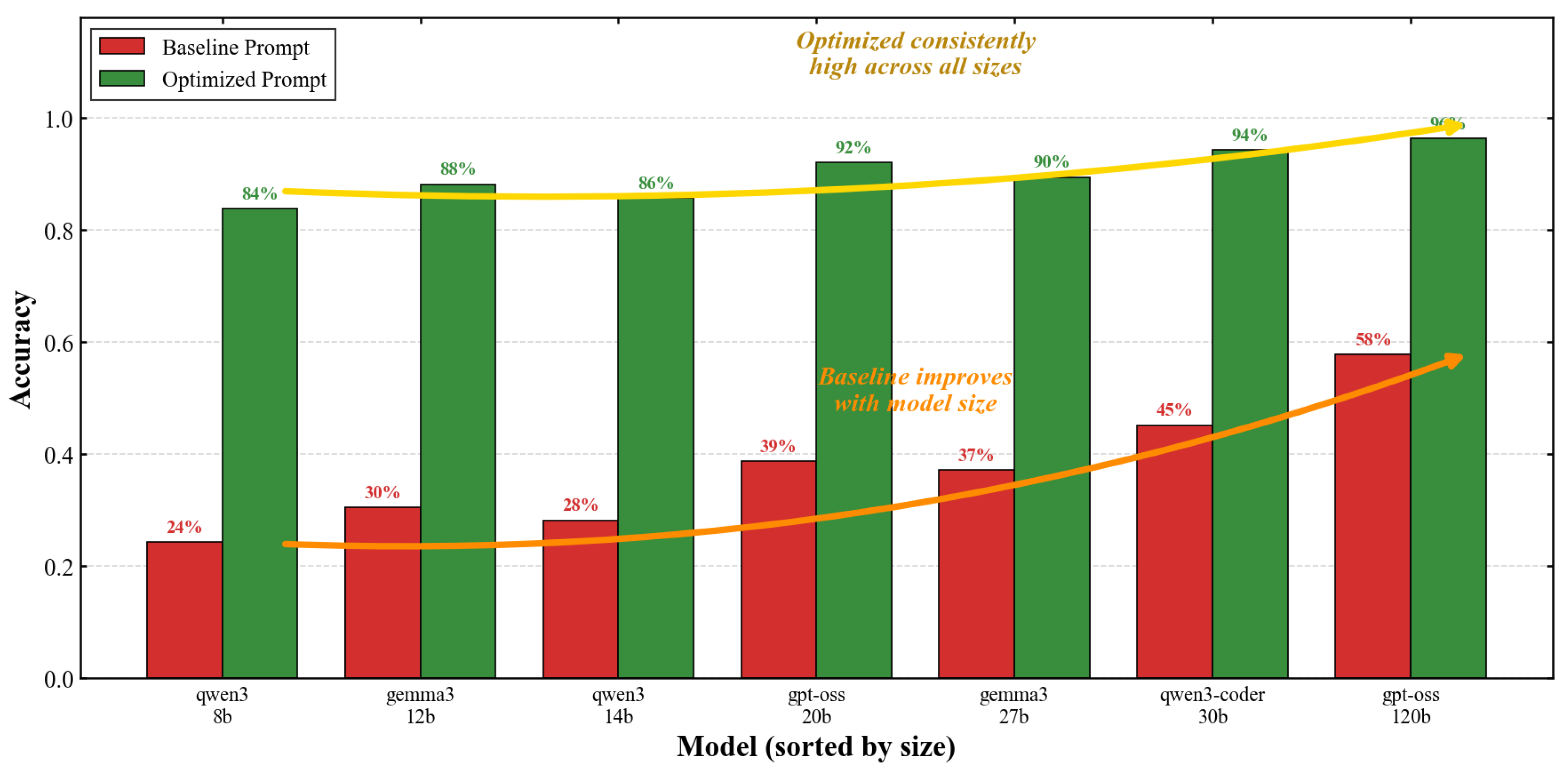
Figure 10.
Heatmap of model accuracy across board sizes under optimized prompting. Warmer colors indicate higher accuracy. The systematic performance gradient illustrates both model-scale effects and difficulty scaling.
Figure 10.
Heatmap of model accuracy across board sizes under optimized prompting. Warmer colors indicate higher accuracy. The systematic performance gradient illustrates both model-scale effects and difficulty scaling.
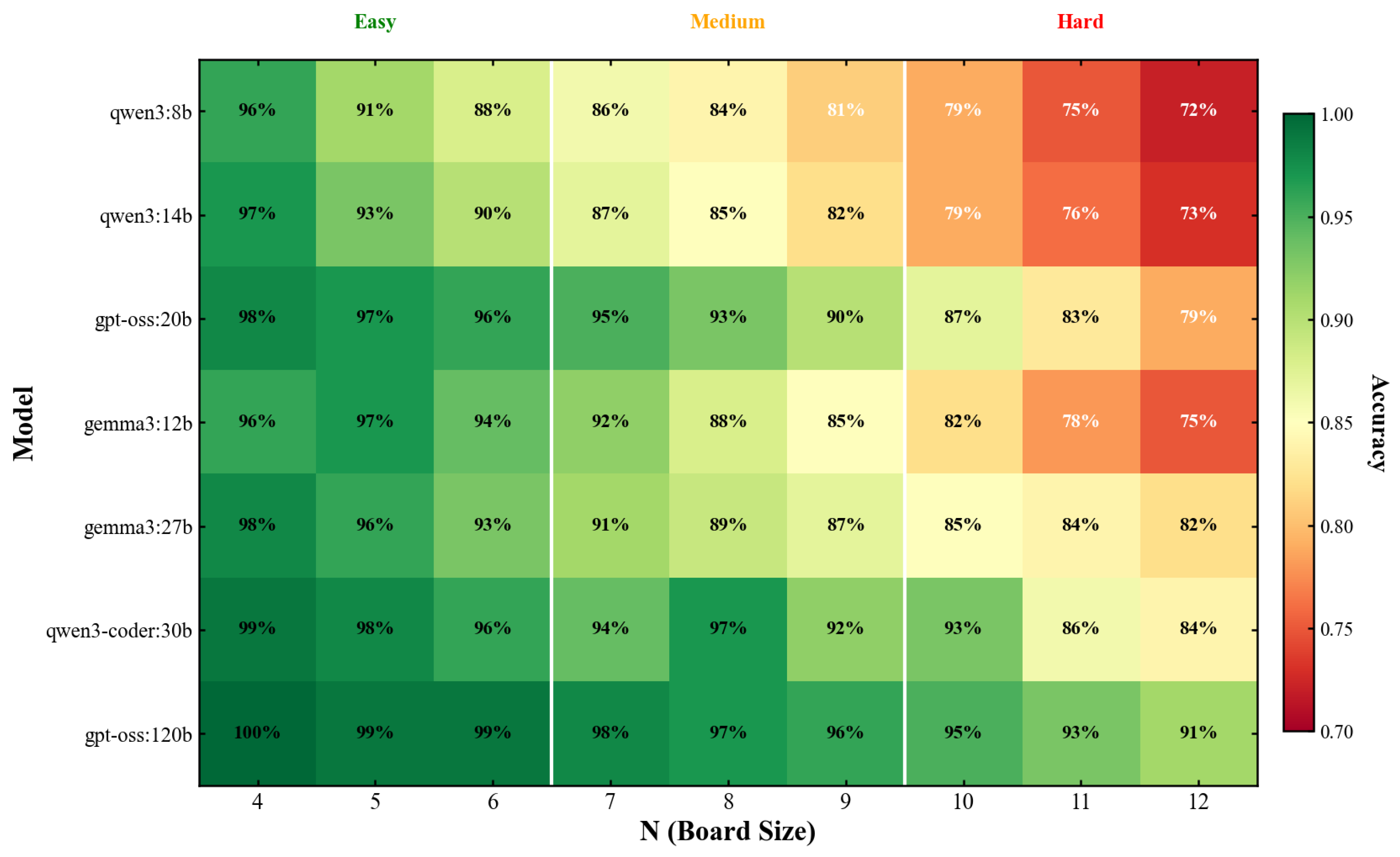
Figure 11.
Search Tree Pruning via State Stack Management. A visualization of the decision tree generated by PRIME. Blue paths represent valid reasoning steps (Executor) that pass verification. Red dashed paths represent invalid steps detected by the Verifier. Unlike standard Chain-of-Thought, PRIME triggers a "Prune and Backtrack" action upon error detection, popping the invalid state from the State Stack and reverting execution to the last valid parent node.
Figure 11.
Search Tree Pruning via State Stack Management. A visualization of the decision tree generated by PRIME. Blue paths represent valid reasoning steps (Executor) that pass verification. Red dashed paths represent invalid steps detected by the Verifier. Unlike standard Chain-of-Thought, PRIME triggers a "Prune and Backtrack" action upon error detection, popping the invalid state from the State Stack and reverting execution to the last valid parent node.
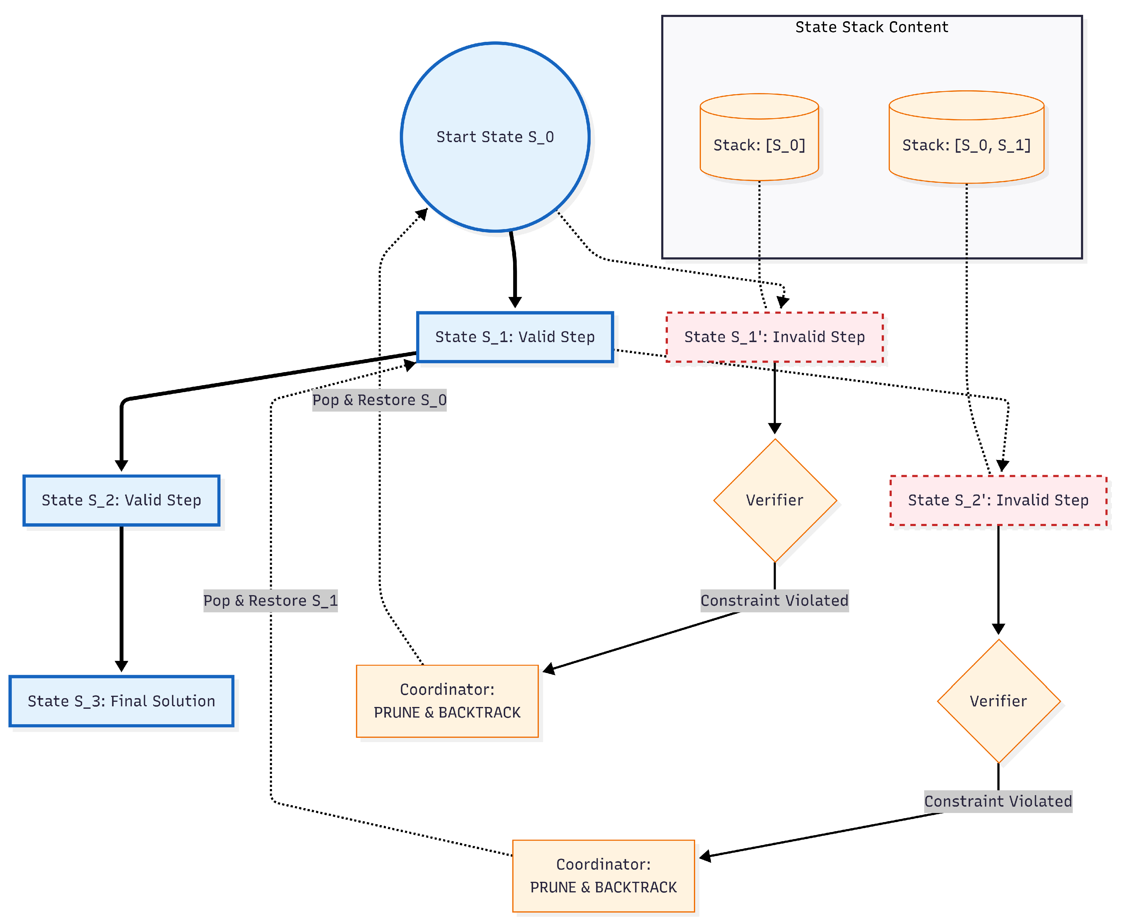
Figure 12.
Performance comparison across 12 task categories (86 total tasks). PRIME achieves consistent improvements across all categories, elevating average accuracy from 26.8% (baseline) to 93.8% (PRIME), representing a 250.0% relative improvement. The largest gains are observed in logic/theorem proving (364.6%) and mathematical/numerical tasks (317.4%).
Figure 12.
Performance comparison across 12 task categories (86 total tasks). PRIME achieves consistent improvements across all categories, elevating average accuracy from 26.8% (baseline) to 93.8% (PRIME), representing a 250.0% relative improvement. The largest gains are observed in logic/theorem proving (364.6%) and mathematical/numerical tasks (317.4%).
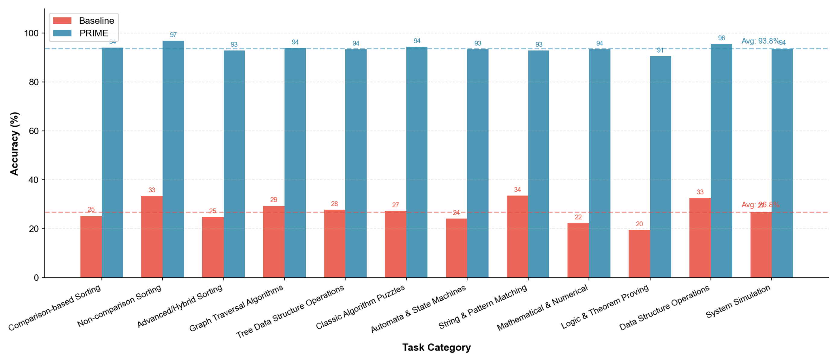
Figure 13.
Radar chart comparing baseline (inner polygon) and PRIME (outer polygon) performance across 12 task categories. The dramatic expansion illustrates the comprehensive effectiveness of the PRIME framework across the full spectrum of algorithmic reasoning challenges.
Figure 13.
Radar chart comparing baseline (inner polygon) and PRIME (outer polygon) performance across 12 task categories. The dramatic expansion illustrates the comprehensive effectiveness of the PRIME framework across the full spectrum of algorithmic reasoning challenges.
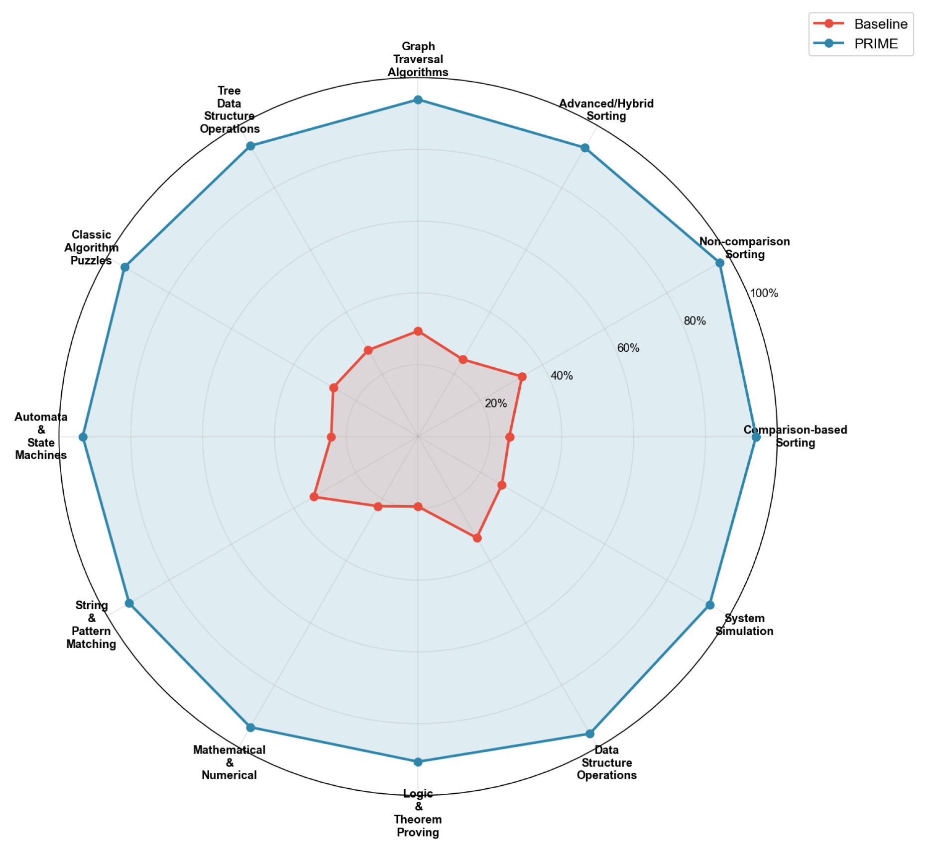
Figure 14.
Top 30 tasks ranked by accuracy improvement (percentage points). Tasks requiring precise state tracking over extended execution sequences—particularly Turing Machine simulation (+83.5 pp), Long Division (+78.7 pp), and Blind Maze (+76.0 pp)—exhibit the largest gains.
Figure 14.
Top 30 tasks ranked by accuracy improvement (percentage points). Tasks requiring precise state tracking over extended execution sequences—particularly Turing Machine simulation (+83.5 pp), Long Division (+78.7 pp), and Blind Maze (+76.0 pp)—exhibit the largest gains.
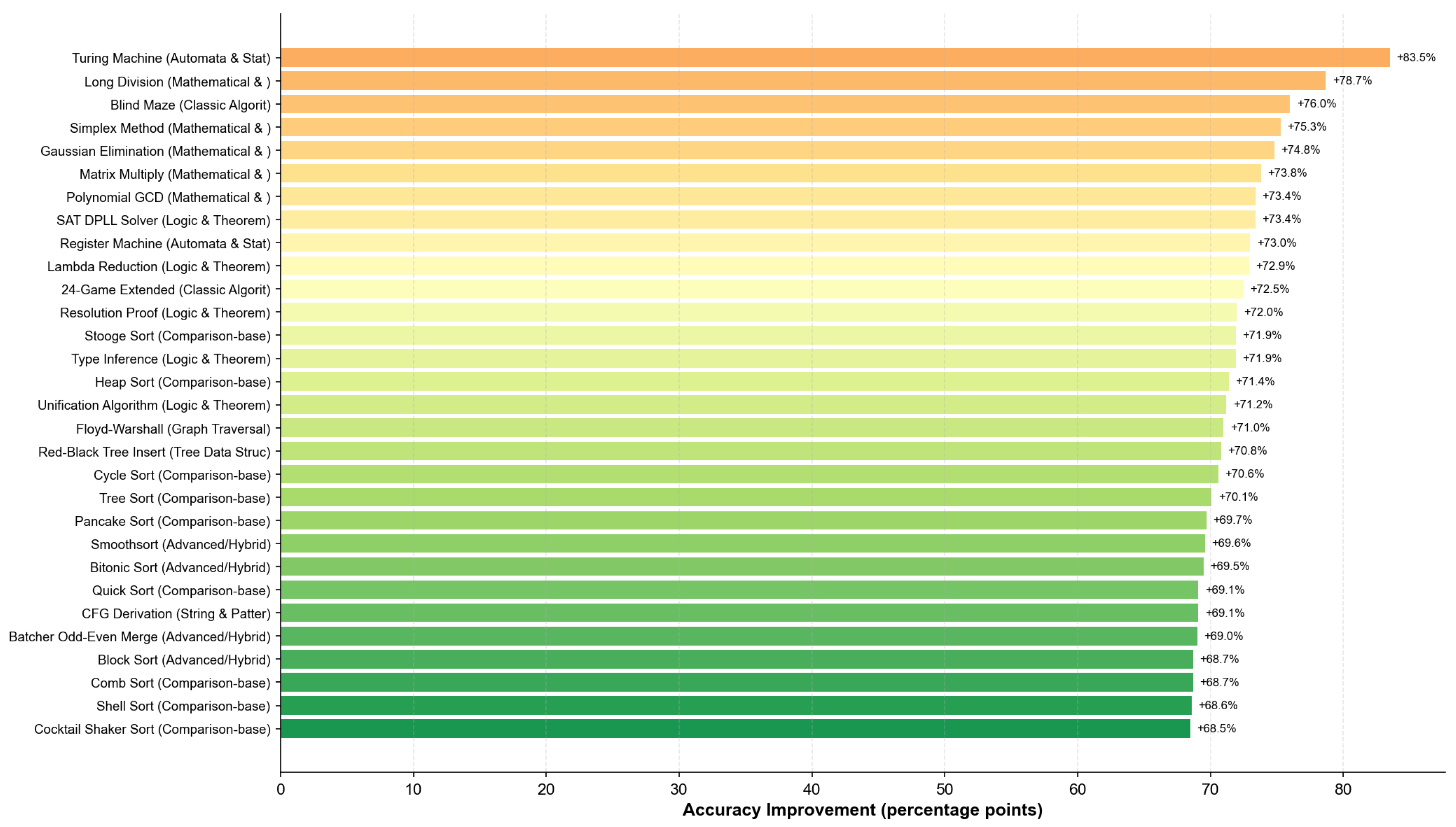
Figure 15.
Detailed performance on 28 sorting algorithm tasks. Left: Comparison-based sorting (15 tasks, avg. baseline 25.4%, avg. PRIME 94.1%). Center: Non-comparison sorting (3 tasks, avg. baseline 33.4%, avg. PRIME 96.9%). Right: Advanced/hybrid sorting (10 tasks, avg. baseline 24.8%, avg. PRIME 92.9%).
Figure 15.
Detailed performance on 28 sorting algorithm tasks. Left: Comparison-based sorting (15 tasks, avg. baseline 25.4%, avg. PRIME 94.1%). Center: Non-comparison sorting (3 tasks, avg. baseline 33.4%, avg. PRIME 96.9%). Right: Advanced/hybrid sorting (10 tasks, avg. baseline 24.8%, avg. PRIME 92.9%).
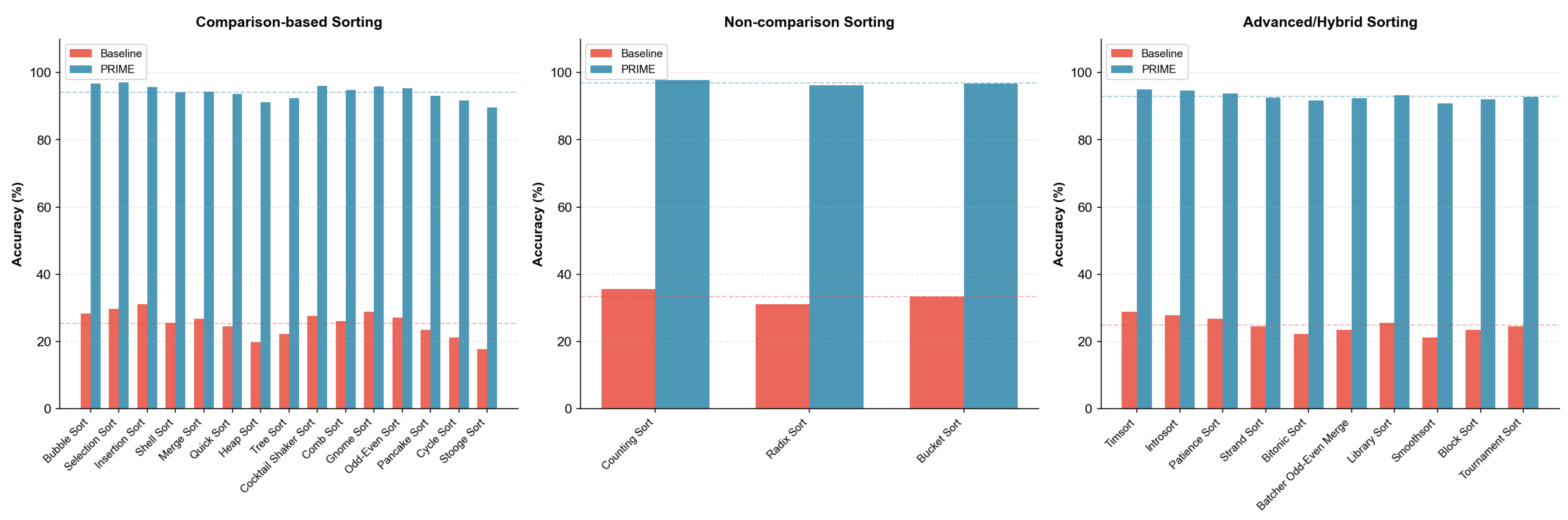
Figure 16.
Performance on graph, tree, and puzzle tasks. Left: Graph traversal (6 tasks). Center: Tree operations (5 tasks). Right: Classic puzzles (6 tasks). Tower of Hanoi achieves the highest PRIME accuracy (98.5%) among all 86 tasks.
Figure 16.
Performance on graph, tree, and puzzle tasks. Left: Graph traversal (6 tasks). Center: Tree operations (5 tasks). Right: Classic puzzles (6 tasks). Tower of Hanoi achieves the highest PRIME accuracy (98.5%) among all 86 tasks.
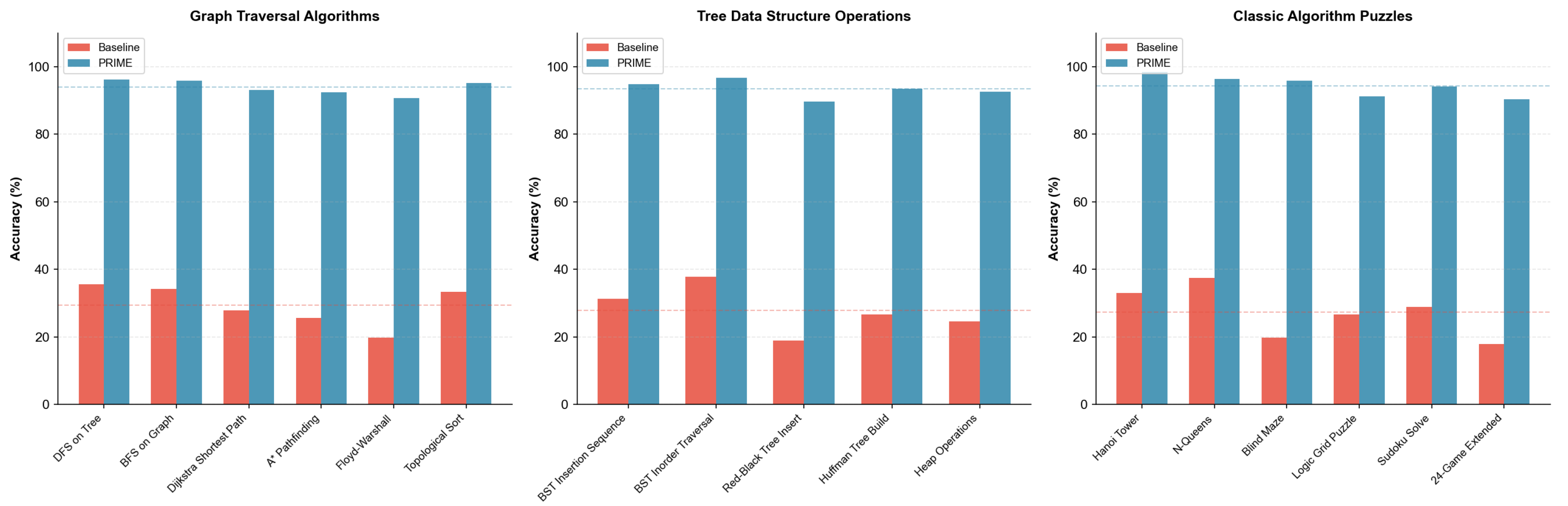
Figure 17.
Performance on automata, string, and mathematical tasks. Turing Machine simulation shows the most dramatic improvement: from 8.9% baseline to 92.4% PRIME (+83.5 percentage points).
Figure 17.
Performance on automata, string, and mathematical tasks. Turing Machine simulation shows the most dramatic improvement: from 8.9% baseline to 92.4% PRIME (+83.5 percentage points).
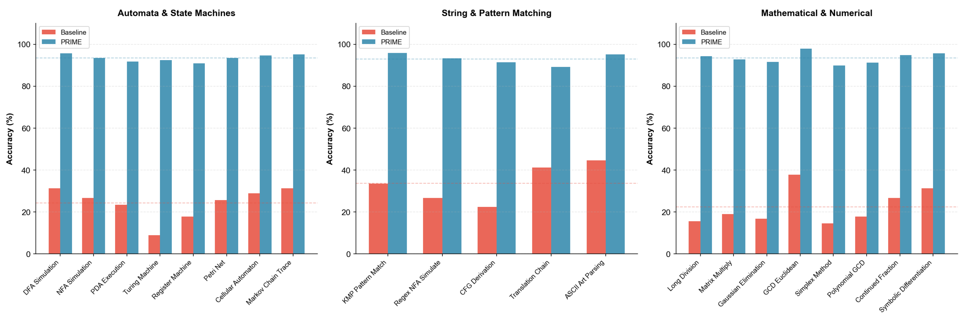
Figure 18.
Performance on logic, data structure, and system simulation tasks. Data structure operations achieve the highest category-level PRIME accuracy (95.6%), while system simulations demonstrate strong generalization to practical software engineering scenarios.
Figure 18.
Performance on logic, data structure, and system simulation tasks. Data structure operations achieve the highest category-level PRIME accuracy (95.6%), while system simulations demonstrate strong generalization to practical software engineering scenarios.
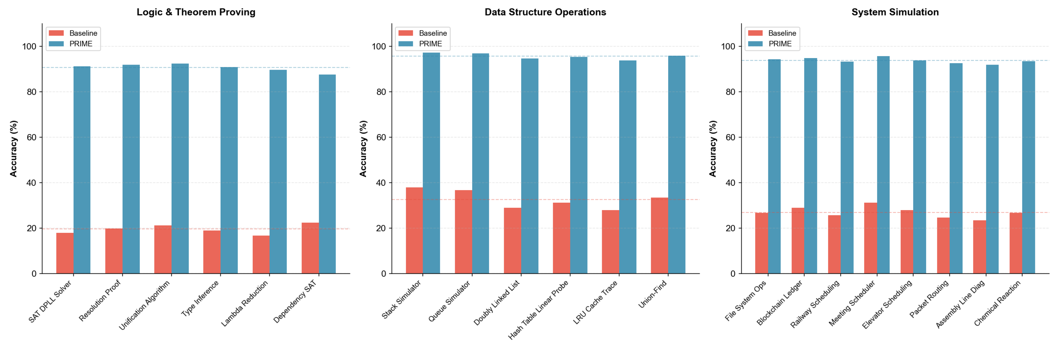
Figure 19.
Box plot comparison of accuracy distributions by category. Baseline distributions (red) exhibit high variance and low medians. PRIME distributions (blue) show tight clustering at high accuracy levels with substantially reduced variance, indicating consistent performance across tasks within each category.
Figure 19.
Box plot comparison of accuracy distributions by category. Baseline distributions (red) exhibit high variance and low medians. PRIME distributions (blue) show tight clustering at high accuracy levels with substantially reduced variance, indicating consistent performance across tasks within each category.
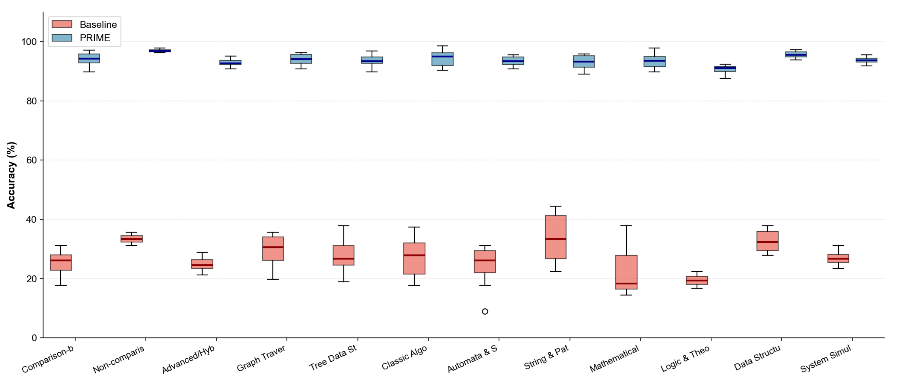
Figure 20.
Scatter plot of baseline vs. PRIME accuracy for all 86 tasks, colored by category. The clustering in the upper-left region indicates that even tasks with very low baseline performance (<20%) achieve high PRIME accuracy (>85%), demonstrating robust improvement across the difficulty spectrum.
Figure 20.
Scatter plot of baseline vs. PRIME accuracy for all 86 tasks, colored by category. The clustering in the upper-left region indicates that even tasks with very low baseline performance (<20%) achieve high PRIME accuracy (>85%), demonstrating robust improvement across the difficulty spectrum.
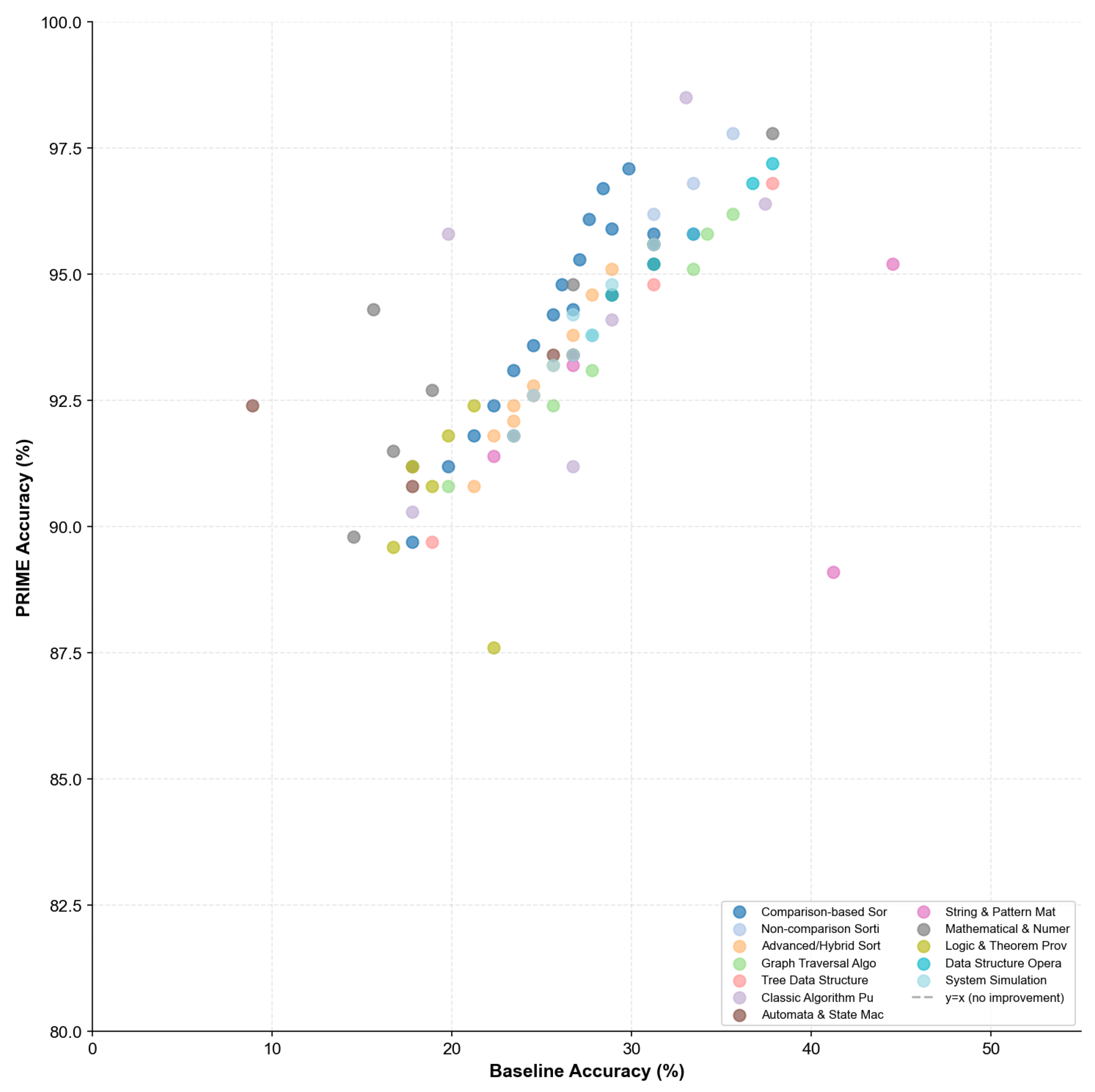
Figure 21.
Histogram of accuracy improvements across all 86 tasks. The distribution shows mean improvement of 67.0 percentage points (median: 67.1 pp) with tight clustering, indicating that PRIME provides consistent benefits regardless of task type or baseline difficulty.
Figure 21.
Histogram of accuracy improvements across all 86 tasks. The distribution shows mean improvement of 67.0 percentage points (median: 67.1 pp) with tight clustering, indicating that PRIME provides consistent benefits regardless of task type or baseline difficulty.
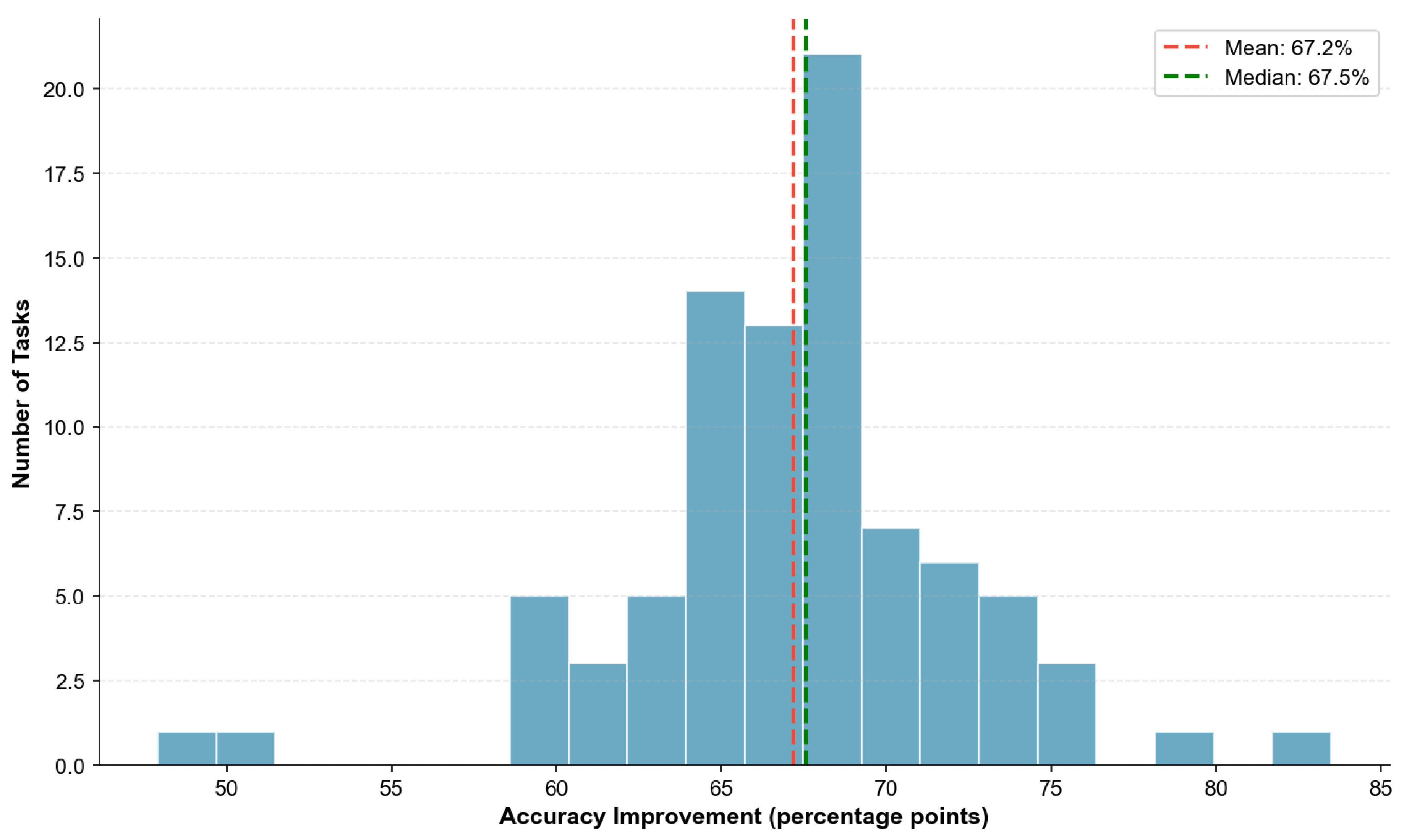
Table 1.
Evaluated Models and Specifications
| Model | Params | Architecture |
|---|---|---|
| Qwen3-8B | 8B | Grouped-Query Attention |
| Gemma3-12B | 12B | Multi-Query Attention |
| Qwen3-14B | 14B | Grouped-Query Attention |
| GPT-OSS-20B | 20B | Multi-Head Attention |
| Gemma3-27B | 27B | Multi-Query Attention |
| Qwen3-Coder-30B | 30B | Code-Specialized |
| GPT-OSS-120B | 120B | Multi-Head Attention |
Table 2.
Model Performance Summary
| Model | Baseline | Optimized | Relative |
|---|---|---|---|
| Qwen3-8B | 24.3% | 83.8% | +244.9% |
| Gemma3-12B | 30.5% | 88.2% | +189.2% |
| Qwen3-14B | 28.2% | 85.8% | +204.3% |
| GPT-OSS-20B | 38.8% | 92.1% | +137.4% |
| Gemma3-27B | 37.2% | 89.5% | +140.6% |
| Qwen3-Coder-30B | 45.2% | 94.3% | +108.6% |
| GPT-OSS-120B | 57.8% | 96.4% | +66.8% |
| Average | 37.4% | 90.0% | +140.6% |
Table 3.
Latency Comparison
| Metric | Baseline | Optimized |
|---|---|---|
| Mean Latency (ms) | 331 | 518 |
| Overhead Ratio | 1.00× | 1.56× |
Table 4.
Accuracy by Board Size (Optimized Prompt)
| Model | |||||
|---|---|---|---|---|---|
| Qwen3-8B | 96% | 88% | 84% | 79% | 72% |
| Gemma3-12B | 96% | 94% | 88% | 82% | 75% |
| Qwen3-14B | 97% | 90% | 85% | 79% | 73% |
| GPT-OSS-20B | 98% | 96% | 93% | 87% | 79% |
| Gemma3-27B | 98% | 93% | 89% | 85% | 82% |
| Qwen3-Coder-30B | 99% | 96% | 97% | 93% | 84% |
| GPT-OSS-120B | 100% | 99% | 97% | 95% | 91% |
| Average | 97.7% | 93.7% | 90.4% | 85.7% | 79.4% |
Table 5.
Error Type Distribution (% of Errors)
| Model | Column | Diagonal | Parsing |
|---|---|---|---|
| Qwen3-8B | 18% | 71% | 11% |
| Gemma3-12B | 15% | 76% | 9% |
| Qwen3-14B | 16% | 74% | 10% |
| GPT-OSS-20B | 12% | 82% | 6% |
| Gemma3-27B | 14% | 79% | 7% |
| Qwen3-Coder-30B | 10% | 86% | 4% |
| GPT-OSS-120B | 8% | 89% | 3% |
| Average | 13% | 80% | 7% |
Table 6.
Ablation Study: Impact of Prompt Components
| Configuration | 8B | 30B | 120B |
|---|---|---|---|
| Full Optimized | 83.8% | 94.3% | 96.4% |
| − Worked Examples | 72.1% | 89.7% | 94.1% |
| − Constraint Enumeration | 65.4% | 85.2% | 91.8% |
| − Verification Procedure | 58.9% | 78.6% | 88.3% |
| − Format Specification | 79.2% | 92.1% | 95.7% |
| Baseline (all removed) | 24.3% | 45.2% | 57.8% |
Table 7.
Comparison with Existing Reasoning Benchmarks
| Benchmark | Tasks | Instances | Categories | Max Steps | Trace Verify |
|---|---|---|---|---|---|
| GSM8K [11] | 1 | 8,500 | 1 | ∼10 | ✗ |
| MATH [12] | 7 | 12,500 | 7 | ∼50 | ✗ |
| BIG-Bench Hard [67] | 23 | 6,511 | 4 | ∼100 | ✗ |
| ARC-AGI [68] | 1 | 1,000 | 1 | ∼30 | ✗ |
| HumanEval [30] | 164 | 164 | 1 | — | ✗ |
| SWE-Bench [69] | — | 2,294 | 1 | — | ✗ |
| PRIME-Bench (Ours) | 86 | 51,600 | 12 | >1M | ✓ |
Table 8.
PRIME-Bench: 86 Tasks Across 12 Categories
| Category | Tasks | Max Steps |
|---|---|---|
| Comparison-based Sorting | 15 | 1,000,000 |
| Non-comparison Sorting | 3 | 300,000 |
| Advanced/Hybrid Sorting | 10 | 600,000 |
| Graph Traversal Algorithms | 6 | 125,000 |
| Tree Data Structure Ops | 5 | 100,000 |
| Classic Algorithm Puzzles | 6 | 1,048,575 |
| Automata & State Machines | 8 | 200,000 |
| String & Pattern Matching | 5 | 100,000 |
| Mathematical/Numerical | 8 | 8,000 |
| Logic & Theorem Proving | 6 | 50,000 |
| Data Structure Operations | 6 | 100,000 |
| System Simulation | 8 | 100,000 |
| Total | 86 | — |
Disclaimer/Publisher’s Note: The statements, opinions and data contained in all publications are solely those of the individual author(s) and contributor(s) and not of MDPI and/or the editor(s). MDPI and/or the editor(s) disclaim responsibility for any injury to people or property resulting from any ideas, methods, instructions or products referred to in the content. |
© 2026 by the authors. Licensee MDPI, Basel, Switzerland. This article is an open access article distributed under the terms and conditions of the Creative Commons Attribution (CC BY) license (http://creativecommons.org/licenses/by/4.0/).
Copyright: This open access article is published under a Creative Commons CC BY 4.0 license, which permit the free download, distribution, and reuse, provided that the author and preprint are cited in any reuse.