
Submitted:
06 January 2026
Posted:
07 January 2026
You are already at the latest version
Abstract
This paper features a 1000 simulations of a set of 100 levered companies equity returns in a financial market. The goal was to generate a realistic distribution of company values that follow a Zipf-Mandelbrot power law. The returns should exhibit leverage effects, negative skewness, and feature Black Swan events of correlated down-turns. Realistic positive covariance structures of returns, systematic risk, plus evidence of long-memory properties. The Merton Model and two versions of the Platen Benchmark Asset Pricing Model (BAPM), the original model and the Stochastic Benchmark Process (SBP). The required market attributes were successfuly captured but the models proved to be highly sensitive to the chosen parameters. The BAPM model proved to be more flexible than the Merton Model and the SBP version more readily generated the stipulated financial market characteristics.
Keywords:
Merton model
; Bench Mark Asset Pricing
; power law
; Zipf-Mandelbrot
; jump-diffusion
; leverage
; cross-correlations
1. Introduction
This paper features a computer simulation of a financial market populated by 100 levered companies. The intention of the simulation is to produce statistical features that characterise financial markets, such as financial return distributions with fat tails and skewness, power law distributions of firm size, financial leverage effects, positive cross-correlations of financial returns, and ’Black Swan’ events in the form of correlated financial market down-turns, Taleb (2008), plus return histories that demonstrate the presence of long memory.
Two basic major different asset pricing models sit at the centre of the simulations, the Merton (1974) model, and the Bench Mark Asset Pricing Model (BAPM), of Platen (2004 a, 2004 b). Two versions of the latter were featured in the simulations. The second aim of the study is to provide an evaluation of which of these two modeling approaches more readily lends itself to a simulation exercise and produces the more realistic financial market characteristics. A more recent version of the BAPM by Platen (2024), referred to as the Stochastic Pricing Model (SPM) proved to more accurately reflect the desired market characteristics. Thus, a total of three different forms of models featured in the simulations.
The Merton model is a structural model of default, based upon option pricing theory, and fundamental to credit risk analysis, as stipulated by the Bank for International Settlements in the Basel Accords. By contrast, the BAPM model of Platen (2004a, 2004b), is based on fewer assumptions than the classical mathematical finance theory, as presented, for example by Jarrow (2022). The BAPM approach employs the growth optimal portfolio (GOP) as a num´eraire and the real-world probability measure as the respective pricing measure.
In practice, it is not easy to implement real-world pricing because the GOP of the entire financial market is a highly leveraged portfolio and is difficult to approximate by a guaranteed strictly positive portfolio. In response to this difficulty, Platen (2024) proposed the concept of benchmark-neutral (BN) pricing which employs the GOP of the market formed by the stocks (without the savings account) as a num´eraire. This is the basis of the SPM used in the study.
The GOP is interchangeably called the Kelly portfolio, expected logarithmic utility-maximizing portfolio, or num´eraire portfolio; see Kelly (1956). The main assumptions for obtaining the real-world price of a contingent claim are extremely weak and consist of the existence of the GOP and the existence of the real-world conditional expectation of the contingent claim when denominated in the GOP; see Platen & Heath (2006) and Du & Platen (2016). This model proved to be the one more generally readily amenable to simulation in the R environment that the authors adopted to conduct the simulation, and in particular the (SPM) version of it.
There are a variety of views about the nature and role of simulations in the generation of knowledge. Alvarado (2023, p1) compares the use of simulations to the development of scientific instruments as a tool of science and he draws a comparison with Galileo’s use and promotion of the telescope. He further suggests that equation-based simulations are the product of several transformations of complex mathematical procedures into something that can be machine implemented and displayed in a humanly intelligible manner.
He cautions that there is a dichotomy of viewpoint in that either computer simulations are seen as being like mathematical and scientific models, or they are viewed as being like experiments. He concludes by suggesting that computer simulations are located some where in between theory and experiment. He returns to the suggestion that they are instruments because they are in-between theory and experiment and because instruments are a third element of inquiry that is situated in between theory and experiment.
Humphreys (2008) adopts a more radical view of the role of simulations because he suggests that computational science introduces new issues into the philosophy of science given that humans are moved from being the centre of the epistemological enterprise to taking a less pronounced role. Science has been traditionally viewed as being a method adopted and carried out by humans. He further describes a situation in which humans deal with science that is carried out at least in part by machines as being a hybrid scenario and also suggests a more extreme situation of a completely automated science that he termed the automated scenario.
These distinctions are even more acute in 2025, because his publication pre-dated the development of Artificial Intelligence (AI), large language models, and unsupervised learning in the context of neural nets. Thus, these dichotomies become even more pronounced in current circumstances.
However, the aim of the current study is not to engage in epistemological debate about the role and value of simulations, but to run a simulation exercise within the R environment, to base it around two distinct asset pricing models, and to then evaluate which one of them more readily produces results which reflect observed attributes of financial markets.
The paper is divided into four section, following this introduction, the models and research methods adopted in the simulation are described in section 2, the results are presented in section 3, and the conclusions follow in section 4.
2. Models and Research Method
2.1. Power Laws
Gabaix (2009) notes that power laws describe the form taken by a large number of empirical regularities encountered in economics and finance. A power law is described by the relation , where X and Y are the variables of interest, is called the power law exponent and K is a constant.
Yule (1925) utilised a power law to describe the evolution of species. The law has been applied to describe numerous phenomena in economics and finance. Gibrat (1931) developed a rule of proportionate growth or the law of proportionate effect, suggesting that the proportional rate of growth of a firm is independent of its absolute size. Prais (1976) applied it to the size distribution of manufacturing firms in the UK. It has been applied to city sizes, the distribution of income and wealth, and stock market activity, to name but a few areas.
Zipf’s law, is a particular case of a distributional power law. Pareto (1896) found that the upper tail distribution of the number of people with an income or wealth S greater than a large x is proportional to , for some positive number, which implies it can be written:
for some The power law exponent is independent of the units in which the law is expressed.
The linguistic law suggested by Zipf (1932) suggests that it is a power-law distribution on ranked data, in the language case, the frequency of occurence of words, and it was extended by Mandelbrot (1953, 1965).
Thus, a plot of the frequency rank of words contained in a moderately sized corpus of text data versus the number of occurrences or actual frequencies, reveals a power-law distribution, with exponent close to one.
Mandelbrot (1963) also suggested that the Gaussian distributions inherent in Brownian motion should be replaced by another family of probability laws, these he referred to as stable Paretian” distributions, which have a power law exponent less than one. These distributions are characterised by fat tails and excess kurtosis relative to a normal distribution.
To ensure that our simulations realistically mimic the actual distribution of the size of firms in financial markets we apply power laws in the simulations. The Zipf-Mandelbrot law is a static frequency distribution, that when applied to corporate market values, describes the cumulative distribution function (CDF) or the rank-size rule of these values at a single point in time.
2.2. Merton Model
In the Merton model, equity may be viewed as a call option on the firm: since the principle of limited liability protects equity investors, shareholders would choose not to repay the firm’s debt where the value of the firm is less than the value of the outstanding debt; where firm value is greater than debt value, the shareholders would choose to repay, in effect, to exercise their option and not to liquidate. This is an example of a structural model, where bankruptcy is modeled using a microeconomic model of the firm’s capital structure.
The Merton model is given by:
where:
and,
- ,
- E = the value of the company’s equity,
- = the value of the company’s assets in period
- K = the value of the company’s debt,
- t = current time period
- T = Future time period,
- r= risk-free rate of interest,
- N=cumulative standard normal distribution,
- e = exponential term,
- = standard deviation of equity returns.
The Merton model plays a key role in the Basel Accords by providing a quantitative framework to assess the probability of default (PD) of a company. The extension of the Black-Scholes option pricing theory to corporate debt, permits financial institutions to translate market information into insights about credit risk. (See Bank for International Settlement publications
2.3. Implementation of the Merton Model in R Code
2.3.1. The Zipf-Merton Model
At the end of the simulation we require a model in which the size distribution of firm equity values conforms to: The simulation achieves this through the principle of Gibrat’s law, proportional growth, but in the cases of the two models, it is implemented in different ways.
In the Merton/Jump-Diffusion framework, the Zipf distribution for firm size is primarily a result of the Geometric Brownian Motion (GBM), part of the asset process, which mathematically embodies Gibrat’s Law. The firm’s asset value is governed by the Jump-Diffusion SDE, (as previously discussed).
The continuous part, , implies that the ’growth rate’, is independent of the firm’s current size , which is Gibrat’s law. However, the accumulation of many independent, random, proportional growth steps, (the GBM part), over a long period , naturally leads the asset size , towards a log-normal distribution.
The power-law tail is further amplified by the initial condition, which involves setting the initial asset sizes to already follow a power-law before the simulation commences.
The Merton transformation, is highly convex. This non-linearity selectively amplifies the relative sizes of the largest firms while punishing the smaller, high-debt firms, thereby helping to stabilize the Zipf tail. In the final ’Equity Value’ , the primary driver is the stochastic component of the GBM , ensuring that the randomness driving firm size is proportional to the size itself. The final term is a jump term described below in section 2.4.3.
The combination of the processes outined in Table 1 generate the stylized facts describing the financial market that are the goal of the simulation. The Jump-Diffusion asset process is an important component of this.
The simulation using the Merton model embodies the following key features:
- Non-Linearity : The Merton formula is a convex function of . Since the equity is a call option, a small drop in when the firm is close to default causes a much larger proportional drop in .
Table 1. Summary of Assumptions and Methods adopted in the Merton Model Simulation
| Assumption | Implication for Simulation |
| No Arbitrage | The core principle that allows option pricing to be used for equity valuation. |
| Debt is Zero-Coupon | The firm has a single debt liability, that matures at a specific time , requiring a single payment. |
| Complete Information | and are observable (or estimable) by the market. |
| Risk-Neutral Valuation | The formula uses the risk-free rate r because the underlying asset process (Jump-Diffusion) is implicitly priced in a risk-neutral world when applying option theory. |
| Default Mechanism | Default occurs only at maturity if . Equity holders walk away, and Otherwise, equity holders receive |
| Asset Process | In the original Merton model the firm’s assets follow a Geometric Brownian Motion. In the simulation, this is replaced by a more realistic Jump-Diffusion Process. |
- Negative Skewness: The Jump-Diffusion process ensures that the fundamental Asset Value has the potential for large, sudden negative shocks (the jumps). When these shocks occur, the non-linear Merton transformation greatly amplifies the resultant negative returns for equity holders, leading to the negative skewness in equity returns.
- Leverage Effect: When drops (due to a jump or continuous movement), the ratio decreases, pushing the firm closer to default. This effectively increases the firm’s financial leverage (risk of ruin). The Merton model correctly reflects this by showing a corresponding increase in equity volatility for the next period, which is the definition of the Leverage Effect observed in financial data.
This setup successfully generates the Zipf Law (due to the growth dynamics on ) and the Leverage Effect/Negative Skew (due to the Jump-Diffusion combined with the Merton non-linearity).
One potential problem, encountered in the initial set-up of the R code used to generate the simulation, was the problem of very small equity values. This meant that potentially the firm could default in the early stages of the simulation and generate missing values (NAs) when it’s value was set to zero. Calculations within R do not always readily accommodate missing values. To avoid this problem in the initialization of the simulations the firm equity values were set within narrow bands.
We also set a cap on equity returns in the process of the simulation to prevent plot distortion from extreme events.
2.4. Benchmark Asset Pricing Model
The BAPM is a framework for asset pricing that incorporates a more general approach to evaluating financial assets. Platen’s BAPM, often referred to using the GOP or Benchmark Portfolio , is an important framework that addresses limitations in classical models like Black-Scholes by explicitly incorporating stochastic volatility and market incompleteness. The core mathematical framework of the BAPM is that it defines the dynamics of any primary asset by relating it to the Benchmark Asset , which is the GOP—the unique portfolio that achieves the maximum expected long-term growth rate among all investable assets.
The , is modeled as the sum of squares of independent geometric Brownian Motions (GBMs), :
Where each follows a stochastic differential equation (SDE):
where:
- are independent standard Wiener processes (Brownian motions).
- is a constant volatility parameter.
The idea behind the asset pricing equation is that the ratio of an asset’s price to the Benchmark price is a martingale under the Benchmark measure Platen models the asset price using the stochastic density equation (SDE):
where:
- r is the risk-free interest rate.
- is the market price of risk for the Benchmark Asset
- The Benchmark Beta, representing the correlation and sensitivity of asset returns to the Benchmark ’s returns.
- The volatility of the Benchmark asset itself is stochastic: .
In the R code used in both of the simulations for the Merton and BAPM models, the equity value was modeled using a price-to-benchmark ratio :
The ratio (the Merton equity in the structural model, or the price-to-benchmark ratio in the BAPM simulation) is driven by the stochastic volatility derived from the process, introducing the leverage effect where volatility is time-varying and linked to the systemic risk of the market.
2.4.1. Key Assumptions of Platen’s BAPM
The BAPM moves away from the restrictive assumptions of the Black-Scholes model, allowing for a more empirically realistic view of market dynamics. Table 2 provides a summary of the key assumptions and their implications in the simulation of the BAPM.
When these characteristics and relationships are translated into R code for the purposes of the simulation, typical market characteristics emerge more readily than is the case for the Merton model.
2.4.2. The BAPM Model
In the BAPM the generation of Zipf’s law is more ’direct’ and is a consequence of the standard GBM that defines the firm’s assets in this context. In the BAPM simulation, the firm’s Asset Value , is modeled as a simple, correlated GBM (Step 4 in the first code snippet).
This GBM explicitly assumes proportional growth, satisfying Gibrat’s Law.
The solution of this SDE is a log-normally distributed random variable:
Table 2. Summary of Assumptions and Methods adopted in the BAPM Simulation
| Assumption | Implication for Simulation |
| Existence of a Benchmark (The GOP). There exists a unique, attainable, self-financing Growth Optimal Portfolio in the market. This portfolio is a true measure of the market, and its growth rate is the maximum achievable long-term growth rate. | Asset pricing is done relative to the , not just the risk-free rate, which is why the -adjusted price is a martingale. |
| Stochastic Volatility and Incompleteness. Market volatility is not constant but is a stochastic process driven by . This allows for volatility clustering and fat tails in returns, matching real-world data. | Unlike Black-Scholes, the market is incomplete. Risk cannot be perfectly hedged solely using the risk-free asset and the underlying asset. The Benchmark is required to define a reference for pricing. |
| Generalized Risk Premium. The expected excess return of any asset over the risk-free rate is proportional to its Benchmark Beta multiplied by the Benchmark’s excess growth rate . | This forms a generalized Capital Asset Pricing Model (CAPM) where the market portfolio is replaced by the . The risk premium is based on the covariance with the process. |
| Time-Dependent Distributions. | The model, because of the process, leads to asset returns that are not log-normally distributed but exhibit leptokurtosis (fat tails) and potentially skewness, which is consistent with the empirical evidence of financial returns. |
Second block of code:
In the expression above, ,, is the drift rate, or the expected return of the asset value, is the volatility of the continuous part of the equation, is a standard Weiner process or Brownian motion. The final term is a jump term, described in the next subsection.
2.4.3. The Jump Process
The third term in the previous equation describes the jump term. is a Poisson counting process that dictates the number of jumps occurring up to time t, and is the random size of the j-th jump, modelled as a log-normal jump factor such that is normally distributed.
The model is based on Kou (2002), who explains that his model is based on a double exponential jump diffusion model. The model has the advantage of being ’arbitrage free’, in that it leads to closed-form solutions for standard option prices, it is able to reproduce the leptokurtic feature of the return distribution, responsible for the ’volatility smile’, and it is possible to interpret the jump part of the model as the market response to outside news.
2.5. Extension of the BAPM to the Stochastic Pricing Model (SPM)
The BAPM (Platen 2004a, 2004b) models the price dynamics of an asset as a product of a benchmark process and the relative price ratio .
The advantage is flexibility, as this framework permits and to be modeled by various stochastic processes (e.g., Brownian motion, jump-diffusion, CIR process for volatility, etc.). The BAPM’s main theoretical goal is to ensure the model produces asset prices that are growth-optimal relative to the chosen benchmark, which addresses the fundamental economic issues of risk-neutral pricing.
2.6. The SBP: A Specific Implementation
The Stochastic Benchmark Process SBP, Platen (2024) is a specific implementation of the BAPM that defines the dynamics of the benchmark using a sum of squared Ornstein-Uhlenbeck processes, which is known to naturally generate several stylized facts. Table 3 describes key components of SBP.
Table 3. Key Features of SBP
| Feature | SBP Model (R Code) | Rationale |
| Benchmark | is the sum of N independent Geometric Brownian Motion processes. | This specific structure naturally yields time-varying volatility |
| Volatility | The process volatility is explicitly derived from the volatility | This links the asset’s risk directly to the state of the benchmark, ensuring the consistency of the BAPM framework. |
In the simulations that follow, we used two versions of BAPM, the base case BAPM and the SBP.
2.7. Comparison of the Generation of the Leverage Effect in the Merton Model and BAPM
The Merton/Jump-Diffusion Structural Model and the Platen (BAPM) achieve the empirically observed leverage effect through fundamentally different economic and mathematical mechanisms. The Leverage Effect is the empirical observation that volatility increases after negative returns and decreases after positive returns.
Table 4 provides a summary of the differences in their generation in the two models used in the simulation.
Table 4. Comparison of the Generation of the Leverage Effect
| Feature | Merton/Jump-Diffusion Model | Platen Benchmark Asset Pricing Model (BAPM) |
| Mechanism Type | Structural / Micro-Economic | Systemic / Macro-Economic |
| Core Driver | Financial Leverage Amplification. | Stochastic Volatility (GOP). |
| Mathematical Cause | The non-linearity (convexity) of the Merton option pricing function | The inversion of the Benchmark Volatility and the correlation between and shocks. |
| Trigger Event | A drop in the firm’s Asset Value, regardless of the cause (continuous or jump). | A drop in the Benchmark Asset (market-wide systemic risk event). |
| Logic Chain | Financial leverage Equity Volatility ↑ (since equity becomes a deeper out-of-the money option on | Market Volatility This high market volatility is then directly imported to drive the asset’s Equity Volatility. |
| Code Implementation | Implicit: Generated by re-calculating the option price based on the new, lower (Step 1 in the second code snippet). | Explicit: Generated by setting and using the global market shock to drive (Steps 5 & 6 in the first code snippet). |
2.7.1. The Merton Leverage Effect
In this model, the leverage effect is a consequence of the firm’s capital structure and the debt contract (financial leverage). The volatility of the firm’s equity is mathematically related to the volatility of its assets by the derivative of the Merton formula:
where is the firm’s financial leverage ratio, and , which is the probability of survival, or the call option delta, which represents the sensitivity of the equity to asset value changes.
When a negative equity return occurs and drops, financial leverage increases, and given that all values in the expression are positive, the equity volatility , increases in the next period.
The inclusion of the Jump-Diffusion process simply ensures that the negative returns are frequent and large enough to consistently trigger this structural leverage mechanism.
2.7.2. Platen BAPM: Systemic Volatility Effect (Stochastic Volatility) and Leverage Effect
In the BAPM, the leverage effect arises from the fundamental dynamics of the market’s benchmark portfolio , which serves as the underlying source of market-wide stochastic volatility.
Key components of this are that the volatility of the Benchmark Asset is inversely proportional to its value:
In situations in which the market drops or the growth optimal portfolio experiences negative returns, the market’s fundamental volatility increases.
There is a direct asset volatility link in that the volatility of the price to benchmark ratio that ultimately drives the equity price is linked to the systemic market volatility :
Since the equity return is a combination of the Asset return and the process, a drop in the market leads to high systemic volatility , which in turn leads to high subsequent volatility in the equity returns. The negative correlation applied between the innovation and further ensures that a market drop coincides with a drop in the price-to-benchmark ratio , locking in the asymmetric relationship between returns and volatility.
The BAPM provides a more fundamental explanation for the leverage effect, linking firm-level volatility directly to the level of market-wide systemic risk.
2.8. The Modelling of Zipf-Mandelbrot Law
The Zipf-Mandelbrot law is a three-parameter generalization of the simpler Zipf’s law . It models the size of an item (firm size or absolute return magnitude) based on its rank , where ranks are ordered from largest to smallest
The general formula is:
where:
- The size (e.g., final equity value or absolute return magnitude) of the firm/event with rank
- : The rank of the item (e.g., 1 for the largest firm, 2 for the second largest, etc.).
- (Exponent): The critical parameter representing the slope in a log-log plot. For Zipf’s law to hold, should be close to .
- (Constant): A scaling constant related to the size of the largest firm/event .
- (Mandelbrot Parameter): A parameter that shifts the rank and is used to account for deviations from the strict power-law, especially for the top few ranks (the head of the distribution).
2.8.1. Linearization for Fitting: Log-Log Regression
Directly fitting the ZM model using non-linear least squares (nls in the R code) can be sensitive to initial guesses and challenging for large datasets. A common method, which is employed to initiate starting values, is to take the logarithm of the simpler Zipf relationship :
This transforms the power-law relationship into a linear relationship in a log-log space:
where slope
The R code employed uses a linear fit (log_fit <- lm(log(Abs_Return) ~ log(rank), data = top_returns))to get initial estimates for and before attempting the more complex Zipf-Mandelbrot fit.
2.8.2. Interpretation of the Fitted Parameters
The Zipf-Mandelbrot fit. is performed for two types of data in the simulation: Final Equity Size and Absolute Return Magnitude.
Final Equity Size (analysis 3 in the R Code).
- Data: = Final Equity Value at time T, ranked by size.
-
Expected Result: For Gibrat’s law to hold perfectly, the fitted exponent should be close to 1.
- −
- If (flatter slope), it suggests growth is slightly less proportional than Gibrat’s Law assumes, potentially favoring smaller firms.
- −
- If (steeper slope), it suggests growth is slightly more proportional than Gibrat’s Law assumes, aggressively favoring the largest firms.
The log-log plot provides a strong visual confirmation, where the fitted line’s slope is the estimate of
Absolute Return Magnitude (Analysis 2 in the R Code )
- Data: (magnitude of returns), ranked by size.
- Test: Does the magnitude of changes in firm size follow a power-law, indicating fat tails in the return distribution?
-
Expected Result: Financial data often exhibits a power-law in the tails of the return distribution. The estimated exponent is typically found to be between and (known as Pareto or Stable distributions), indicating much fatter tails than the normal distribution
- −
- A smaller means fatter tails and more extreme events.
- −
- The Jump-Diffusion model is designed specifically to generate these fat tails, which should be reflected in a significantly small value in this fit.
In summary, the Zipf-Mandelbrot model is the formal test that links the underlying Gibrat’s Law assumption of the simulation to the empirically observed power-law distributions of firm size and return magnitude.
2.9. The Determination of Market-Related Risk or Cross-Correlation
The goal is to calculate the pairwise correlation coefficient between the equity returns of every single firm i and firm j over all simulated time periods.
A. Return Matrix Preparation.
- Time Series Extraction: The simulation first extracts the time series of Equity Returns for every firm i (where across all time periods t (where .
- Wide Format Conversion: This data is organized into a large matrix, where T is the number of periods and Nis the number of firms.
The R code uses pivot_widerto create this matrix (returns_wide_clean)
B. Correlation Matrix Calculation
The correlation matrix is an matrix where each off-diagonal element is the sample correlation coefficient between the return series of firm i and firm j.
The correlation coefficient is calculated using the standard formula:
where is the sample covariance between the returns of firm i and firm j, and and are the sample standard deviations of the returns for firm i and firm j.
The R code generates this directly using correlation_matrix <- cor(returns_wide_clean).
C. Heatmap Visualization and Interpretation
The heatmap provides an immediate visual answer to the question: To what degree are the returns of all firms moving together?
- Color Intensity: The color gradient (e.g., green for positive, red for negative, white for zero) visually represents the magnitude and sign of .
- Uniformity: A successful simulation of systemic risk should show a predominantly uniform positive color across the off-diagonal elements, indicating that all firms are exposed to a common, market-wide shock. This is characteristic of the real equity market.
2.9.1. Systematic Risk in the Simulation Models
The common, systemic component is introduced differently in the two simulation models, but the heatmap should capture it equally well. The mechanisms adopted are presented in Table 5 below.
Table 5. The capturing of Systemic Risk
| Model | How Systemic Risk is Introduced | What the Heatmap Confirms |
| Merton/Jump-Diffusion | A single global market shock is used to correlate both the continuous GBM component and the jump magnitude across all firms via Jump_Correlation_Rho (set at 0.60) | If the Jump_Correlation is high it suggests the simulation successfully generated a high, uniform cross-correlation among all firms. |
| Platen BAPM | A single global market shock drives the Asset process and also drives the Benchmark and processes. | Whether the combined effects of the correlation and the systemic volatility successfully resulted in a uniform positive cross-correlation structure. |
Many iterations of these models were simulated using slightly different parameter settings. The results presented in the next section four represent those that the authors thought that best captured market realities. The R Code reported reflects these settings.
2.10. Time Series Properties of the Models
The long memory properties of financial return series are characterized by the persistence of observed autocorrelations over long time periods. This phenomenon has been observed in various financial markets, including stock markets, FOREX, and commodity markets, and is higher at lower frequencies (daily, weekly, and monthly). Engle (1982) used this feature to develop the autoregressive conditional heteroskedasticity (ARCH) model which is a statistical model for time series data that describes the variance of the current error term or innovation as a function of the actual sizes of the previous time periods’ error terms. Bollerslev (1986) generalised the model to the generalised autoregressive conditional heteroskedasticity (GARCH) model by introducing an auto-regressive moving average (ARMA) component.
Another approach to measuring volatility is to measure it directly from observed price changes. Realized volatility (RV), developed by Barndorff-Nielsen and Shephard (2002), is a statistical measure that quantifies the actual variability or fluctuations in the price of an asset over a defined timeframe. Unlike implied volatility, which reflects market expectations of future price movements, realized volatility is based on observed historical data, usually high frequency within the day observations at 5 minute or 15 minute intervals.
Corsi (2009) introduced a simple and easy-to-implement model called the heterogeneous autoregressive (HAR) model. This model utilizes the past daily, weekly, and monthly RVs called 1, 5, and 22 lags, respectively, as variables to predict future volatility.
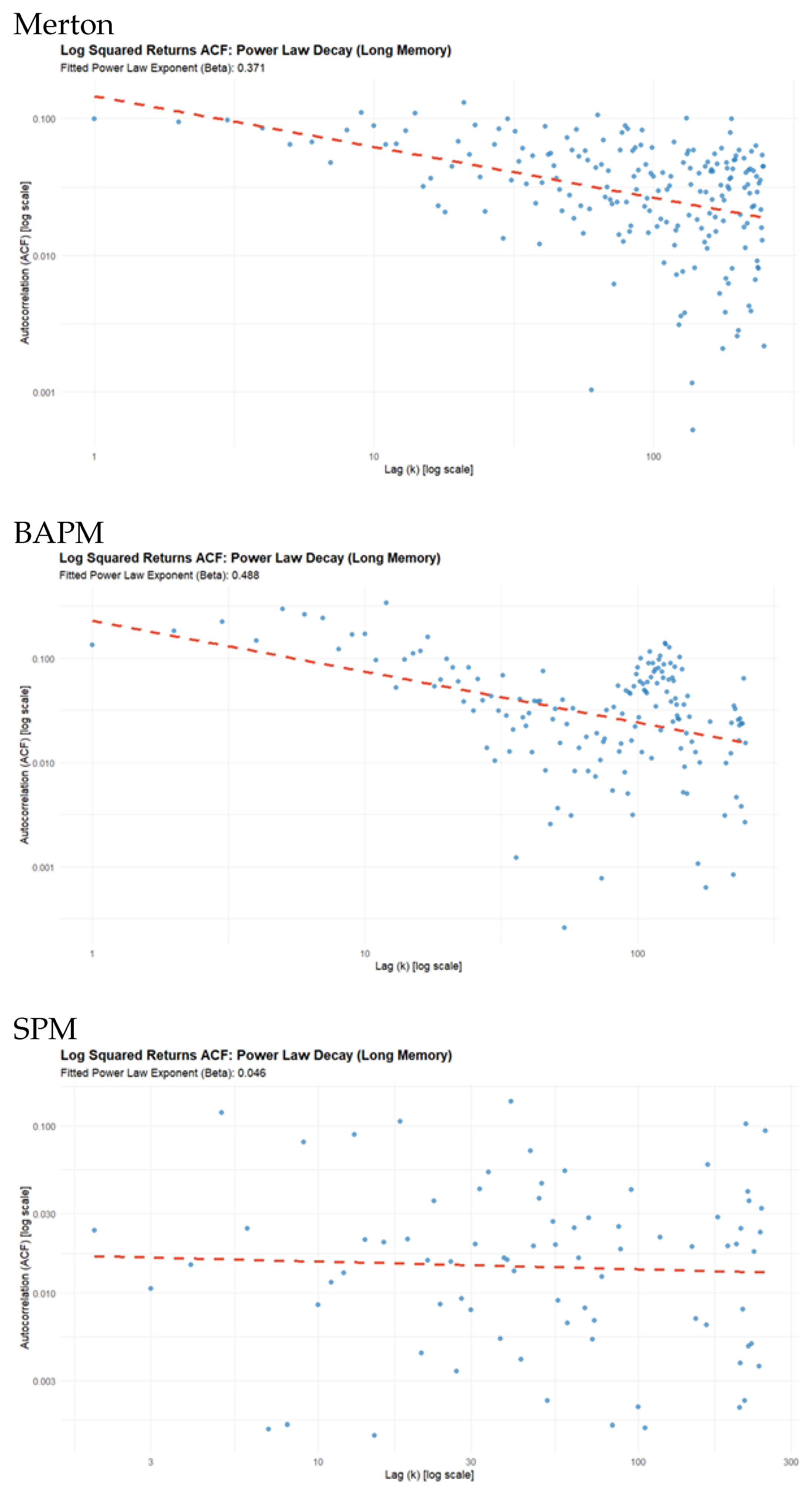
The standard way to check for long memory in volatility is to plot the Autocorrelation Function (ACF) of the squared returns on a log-log scale. If the ACF exhibits a linear decay on this plot, it indicates a power-law decay, which is the definition of long memory (or slow decay of volatility correlations). We utilise this method to check the time-series properties of the returns generated by the three different models used in the simulations.
3. Simulation Results
The objective of this study is to assess the efficacy of three distinct simulation methodologies in replicating the primary stylized facts of equity returns and market structure. Specifically, we compare a basic Merton Jump-Diffusion Model, a Simplified Benchmark Approach Process Model (BAPM) with explicit leverage, and Platen’s advanced Stochastic Benchmark Process (SBP) BAPM. This section presents the comparative results across six key properties: Fat-Tailedness (Kurtosis), the Leverage Effect, Negative Skewness, the Zipf Power Law for firm size, market-wide positive covariance structures, and the presence of long-memory in volatility. The comparison highlights not only the successful emergence of these properties but also contrasts the theoretical superiority of the SBP model, which generates volatility and leverage endogenously from its core structure, against models that require these effects to be explicitly imposed.
3.1. Asset Pricing and Return behaviour
The three pricing models were fine-tuned by running numerous different simulation runs with different parameter settings. The goal was to target the previously described market characteristics. The R code reported matches the parameters used to generate the results reported. The authors acknowledge the assistance of (Google) in the development and refinement of the R code used for this analysis. The Merton model produced equity financial return characteristics with the values shown in Table 6 below.
Table 6. Properties of the equity returns generated by the Merton Model.
| Mean | Standard Deviation | Skewness | Kurtosis | Coefficient of Variation |
| 0.001182 | 0.02296 | 0.497 | 172.5928 | 19.42 |
The measurements of the return, standard deviation and skewness appear to be reasonable, but the kurtosis is far too high.
Table 7 presents the results for the BAPM model and shows that the means, standard deviation, skewness and kurtosis have very reasonable and realistic values. The coefficient of variation is very high with a value of 135.67, but this is because the daily mean is near zero, thus the ratio of volatility (Std Dev) to mean is high.
Table 7. Properties of the equity returns generated by the BAPM Model.
| Mean | Standard Deviation | Skewness | Kurtosis | Coefficient of Variation |
| 0.00068 | 0.09226 | 0.3813 | 2.2174 | 135.67 |
Table 8 presents the results for the SPM model and again shows that the means, standard deviation, skewness and kurtosis have very reasonable and realistic values. The coefficient of variation is very high with a value of 197.97, but this is because the daily mean is near zero, thus the ratio of volatility (Std Dev) to mean is high.
Table 8. Properties of the equity returns generated by the SPM Model.
| Mean | Standard Deviation | Skewness | Kurtosis | Coefficient of Variation |
| 0.000978 | 0.193623 | 0.5807 | 0.8015 | 197.97 |
To facilitate a comparison with actual market parameters we down-loaded a year’s worth of adjusted daily closing prices for five major stocks in the Dow Jones Index, namely Apple, Microsoft, United Health Group, Visa and Johnson and Johnson, for one year terminating on 1st November 2025. Their return properties are shown in Table 9.
Table 9. Financial Return Characteristics of Apple, Microsoft, United Health Group, Visa and Johnson and Johnson.
| Company | Mean | Standard Deviation | Skewness | Kurtosis | Coefficient of Variation |
| AAPL | 0.0007946330 | 0.02044543 | 0.6238346 | 11.136530 | 25.72940 |
| MSFT | 0.0009565097 | 0.01515879 | 1.0108713 | 8.750040 | 15.84803 |
| UNH | -0.0019775136 | 0.03210627 | -2.8401703 | 20.100734 | 16.23568 |
| V | 0.0006245149 | 0.01409472 | -0.5467345 | 7.754523 | 22.56907 |
| JNJ | 0.0007134920 | 0.01223558 | -0.7691757 | 8.999480 | 17.14887 |
The period considered has been marked by a great deal of uncertainty about the implications of President Trump’s combined tariff and foreign policy. Nevertheless, the return behaviour for these five companies is similar to the results of the Merton Model simulation with the exception of the value of the kurtosis. The maximum kurtosis reported in Table 9 is that for United Health with a value of 20.1 whilst the simulation produced a value of 172, which is far too high.
Similarly, though the statistical properties of the BAPM model and SPM are very reasonable, the values of the coefficients of variation, are far too high, for the previously mentioned reasons.
Figure 1 displays QQ plots of the return distributions generated by the three simulations and shows how far they deviate from Gaussian distributions.
The QQ plots of the results of the three simulation models shown in Figure 1 reveal that all the generated return distributions have fat tails, but the results of the Merton model deviates to a greater degree from a Gaussian distribution, as was previously suggested by the high kurtosis value. This is also confirmed by the plots of the three generated distributions which are shown in Figure 2.
The distributions generated by the BAPM and SPM models possesses fat tails but are generally more realistic than the one produced by the Merton model. Why is this?
The problem lies in the fact that the Merton model is a structural model. This meant that to achieve realistic simulations results we had to prevent too many firms defaulting at the start of the simulation. This meant that at the start of the simulation we had to set the debt levels within narrow bands using the following R code.
# FIX 1: Debt levels (D): Adjusted to prevent tiny equity values for small firms
D = A_0 * runif(NUM_FIRMS, 0.65, 0.85) -
(1 - runif(NUM_FIRMS, 0.7, 0.95)) * 100,
Furthermore, we set a strict cap on equity returns, using the following code:
# --- Step 3: Calculate Returns (for t > 1) and BIND results (Includes Return Cap Fix) ---
if (t > 1) {
# Fetch previous period’s equity value for return calculation
prev_equity <- simulation_results %>%
filter(time == t - 1) %>%
pull(Equity_Value)
period_data <- period_data %>%
# CRITICAL: This line creates the ’Equity_Return’ column
mutate(Equity_Return = ifelse(prev_equity <= 1e-6, 0, (Equity_Value - prev_equity) / prev_equity)) %>%
# FIX 2b: Capping returns to prevent plot distortion from extreme events
mutate(Equity_Return = pmin(0.5, pmax(-1, Equity_Return)))
} else {
period_data <- period_data %>%
mutate(Equity_Return = NA_real_)
}
Even with the return cap set at a range between (0.5 and -1.0), the simulation generated distribution is still heavily concentrated around with the outliers clustered at the two boundaries, and this has the effect of producing high kurtosis.
A further important factor driving the fat tails in the simulations is the correlated jump process. To generate significant negative Skewness (the long left tail) and high Excess Kurtosis (fat tails), simply relying on the random movement of individual firms (even within the non-linear Merton framework) was not enough. It was necessary to explicitly introduce a Systemic Jump component—a small probability of a large, correlated negative shock across all firms. This suggestss that market crashes are primarily driven by systemic, shared risk factors, not just the aggregation of independent idiosyncratic risks.
3.2. Zipf-Mandelbrot Law and the Size Distribution of Firms
We wanted to ensure that the size distribution of firms in the simulations followed the Zipf-Mandelbrot law and conformed to what is observed in practice. The Zipf-Mandelbrot law is a static frequency distribution and when applied to corporate market values, it describes the cumulative distribution function (CDF) or the rank-size rule of these values at a single point in time. The law implies: Scale Invariance, or the existence of a Power Law Tail. The distribution indicates that the number of companies with market capitalization greater than M decays according to a power law (for large M). This is often interpreted as evidence of a highly competitive or scale-free market structure, where growth is largely independent of current size (Gibrat’s Law).
To verify this we downloaded the market capitalizations in US dollar terms of 3560 US companies (accessed 21 October 2025 from https://companiesmarketcap.com/). We fitted the following model using Maximum Likelihood estimation in R : . The results are shown in Table 8.
Table 8. Zipf-Mandelbrot Power Law fitted to 3560 US Companies
| Parameters | estimate | t value |
| C | 5.749e+13 | 19.49*** |
| alpha | 1.459 | 99.91*** |
| beta | 4.407 | 40.55*** |
| Pseudo R-Squared | 0.9768 | |
NB:*** indicates signicance at the one percent level.
The estimates of this model recorded in Table 8 suggest that all coefficients are significant at the 1 percent level and the pseudo R-Squared statistic suggests that the model accounts for over 97 percent of the variance. The value of α is 1.459, and this is the estimated power-law exponent (or Zipf exponent).
Since α>1, this indicates that the distribution is heavy-tailed but has a finite mean and a finite variance. This value is typical for firm size distributions, which are often found to have exponents greater than 1. The value of beta is 4.407. This is the Mandelbrot shift parameter. A positive β value suggests the simple Zipf’s Law (β=0) would have over-predicted the size of the very largest firms (Rank 1, 2, 3), and the shift is necessary to better model the entire distribution, specifically the head. C is the scaling constant.
A plot of the fit of the model to the 3560 companies is shown in Figure 3.
Table 9 shows the Zipf-Mandelbrot regression models fitted to the simulations generated by the two models. The fitted values are significant at the 1 percent level. Plots of the Zipf-Mandelbrot power law fits for the two simulation model outputs are shown in Figure 4. The theoretical value of the slopes shown in Figure 4 should be 1. The slope for the Merton Model is 1.158 whilst that for the SPM model is 1.244. Both are close to their theoretical values though the Merton Model is a slightly better fit.
The fit for the BAPM model is poor and the regression was eventually fitted to the absolute value of returns, however, the plot in Figure 4 is to actual firm size.
Table 9. Zipf-Mandelbrot Power Law fitted to the simulated equity capitalizations generated by the two models.
| Merton Model | BAPM | SPM | ||||||
| Parameters | estimate | t value | Parameters | estimate | t value | Parameters | estimate | t value |
| C | 1.475943 | 27.227*** | C | 4.699851 | 105.73*** | C | 7.43078 | 13.98*** |
| alpha | 0.442571 | 60.428*** | alpha | 0.229898 | 121.93*** | alpha | 0.32826 | 28.82*** |
| beta | 3.57604 | 8.737*** | beta | 0.010000 | 0.125 | beta | 59.61363 | 10.42*** |
NB:*** indicates signicance at the one percent level
Figure 4. Zipf-Mandelbrot Power Law fitted to the simulated equity capitalizations generated by the three models.
The standard theoretical Zipf-law implies an alpha value that aprroximates 1 and a beta value that is zero. The regression values reported in Table 9 reflect that the alpha parameter in the Zipf-Mandelbrot Law, relates to the slope of the log-log plot which had slopes of 1.158 for Merton and 1.224 for SPM, and this controls the distribution’s tail behavior—specifically, how fast the market capitalization drops off as firm rank increases.
A lower alpha value of 0.44 and 0.33 respectively, implies a flatter slope on the log-log plot compared to the theoretical alpha value of 1. This means the simulated market is less concentrated than expected. The drop in market capitalization from the largest firm (Rank 1) to the smaller firms (Rank 2, 3, etc.) is slower than expected. In a highly concentrated market (high alphas), a few firms dominate, but in the simulation results for both models, the wealth is distributed more evenly among the largest firms.
The Simplified BAPM (Model 2) provided mixed results regarding the power-law stylized facts, demonstrating the critical need for the sophisticated Stochastic Benchmark Process (SBP) structure. While the model successfully captured the Fat-Tailed property of returns, yielding a highly significant power-law exponent of alpha of 0.2299 for absolute returns magnitude, it fundamentally failed to replicate the Zipf Law for firm size. The linear fit on the final equity capitalization (size) produced an exponent of alpha = 24.241 (Figure 4), which diverges drastically from the empirical expectation of an alpha of approximately 1.0. This failure illustrates that simply enforcing the structure and adding an explicit leverage term is insufficient to model the realistic growth dynamics that lead to power-law wealth concentration. This contrast highlights the theoretical necessity of the SBP (Model 3), which successfully generated a realistic size exponent of alpha 1.244 through its endogenous volatility and growth mechanisms.
3.3. The Leverage Effect
Figure 5 reports plots of the leverage effects produced by the three models. All three models successfully reproduce the Leverage Effect, where volatility increases following negative returns (Figure 5). While the Merton model and the Simplified BAPM (Model 2) show this asymmetry, they achieve it through either an explicit negative correlation or an ad-hoc volatility formula, respectively. The true theoretical contribution is found in the SBP Model (Model 3), where the leverage effect emerges endogenously from the multiplicative structure and the underlying SBP process itself. This endogenous generation of a complex stylized fact provides strong evidence that the SBP framework accurately captures the fundamental, self-reinforcing relationship between a firm’s equity value and its risk profile, making it the most theoretically robust of the three approaches.
3.4. Systematic Risk (Covariance Structure)
A crucial test for any market simulation is the ability to generate realistic Systematic Risk—the small but positive cross-sectional correlation observed between individual firm returns. The simulated Covariance Structure (Figure 6)
for the BAPM model confirms success in this area.The heatmap visually demonstrates that the off-diagonal elements of the correlation matrix are predominantly small and positive, clustering near the white/light-green regions (near 0.0 to 0.5). This realistic pattern of low, positive average correlation confirms that the introduction of a shared Global Market Shock via the correlation parameter successfully embeds systematic risk into the asset dynamics . This outcome contrasts sharply with models that rely solely on uncorrelated Brownian motions, underscoring the BAPM’s capacity to transition successfully from firm-specific dynamics to a realistic, interacting market ecosystem.
3.5. Time-Series Properties of Simulation Returns
We first analysed the time-series properties of the S&P500 Index by downloading five years of daily adjusted closing prices on the index from Yahoo finance (accessed on 9/11/2025), calculating the return series, squaring them as a proxy for volatility. We then performed linear regression on the log-log data, the slope of this line is the negative of the power law exponent (beta). The result of this analysis for the S&P500 Index is shown in Figure 7. The slope is 0.724 in Figure 7, confirming the presence of long memory.
The same analysis was then applied to the results of the three simulation models. The coding sequence had to be slightly different for the three models. In the Merton Model code segment calculates the index returns differently than the BAPM and SBP models. In the Merton model, we simply pull all individual firm returns into a vector called ’all_returns’ and calculate the mean/std dev based on that. In the BAPM/SBP model, we calculate a time series of the Market-Cap Weighted Index Return and call that vector ’index_returns_by_day’. The long memory code in the BAPM/SBP models is based on the single time series of market index returns to test its volatility clustering properties, not a collection of all individual returns.
The results of running the same analyses on the three simulation models is shown in Figure 8.
The results in Figure 8 suggest that the BAPM model is the most successful in capturing the long memory properties of time-series of returns. Its beta value is the highest of the three, with a value of 0.488, followed by MERTON with a value of 0.371, and then SPM with a value of 0.046. This suggests that SPM is not successful in capturing long memory effects.
4. Conclusions
4.1. Technical Conclusions
The objective of this study is to assess the efficacy of three distinct simulation methodologies in replicating the primary stylized facts of equity returns and market structure.
Specifically, we compare a basic Merton Jump-Diffusion Model, a Simplified Benchmark Approach Process Model (BAPM) with explicit leverage, and Platen’s advanced Stochastic Benchmark Process (SBP) BAPM.
The results consist of the comparative performance across six key properties: Fat-Tailedness (Kurtosis), the Leverage Effect, Negative Skewness, the Zipf Power Law for firm size, market-wide positive covariance structures, and the presence of long-memory in volatility. The comparison highlights not only the successful emergence of these properties but also contrasts the theoretical superiority of the SBP model, which generates volatility and leverage endogenously from its core structure, against models that require these effects to be explicitly imposed.
The results consist of the simulations of these three separate models: the Merton Model, BAPM and SPM. Namely, realistic financial return characteristics including skewness, kurtosis and fat tails, systematic risk, correct size distributions, and long-memory effects in risk.
We designed the simulation to attempt to capture the Zipf-Mandelbrot power law characteristics that typify the size distribution of the equity values of actual firms. The behaviour of financial returns was expected to display leverage effects. Firms in aggregate are expected to display positive systematic risk (covariance structure). The simulated financial return series are also expected to display the long memory time-series properties, that GARCH, RV and the HAR model are constructed on.
Table 10 summarizes the performance of the three simulation models in relation to these target objectives. Table 10 suggests the dominance of SBP, and the eventual results also hide the fact that there had to be more conditions imposed in the R coding of the Merton model. This was to ensure that it ran smoothly, did not crash because it generated to many missing values (NAs), yet produced the desired market effects.
All three models successfully reproduce the Leverage Effect, where volatility increases following negative returns (Figure 5). While the Merton model and the Simplified BAPM (Model 2) show this asymmetry, they achieve it through either an explicit negative correlation or an ad-hoc volatility formula, respectively. No model generated negative skewness. The other major failure of SBP was in long-memory effects.
Table 10: Summary of Simulation Results
| Stylized Fact | Empirical Expectation | Merton (Model 1) | BAPM (Model 2) | SBP (Model 3) | Conclusion |
| Size Distribution | Success | Fails | Success | Merton is superior | |
| Negative Skewness | Fail | Fail | Fail | All Fail | |
| Fat Tails (kurtosis) | Too extreme | Success | Success | SBP is superior | |
| Leverage Effect | Negative Returns ↑ Volatility | Success | Success (Explicit) | Success (Endogenous) | All succeed |
| Systematic Risk Correlation Structure | Positive Correlation | Success Heatmap white to green. | Fail. Heatmap white to red. | Success. Heat map mainly green | SBP is superior. |
| Long Memory Effects | Positive power slope | Success | Success | Failure | BAPM is superior |
The true theoretical contribution is found in the SBP Model (Model 3), where the leverage effect emerges endogenously. Another complication is that even when simulation’s random seeding is set to the same value, the outcomes of each run of the simulations are stochastic.
Nevertheless, a pattern emerges from the simulations which seems to favour the SBP model as the one which more readily captures market characteristics.
4.2. Policy Implications
The simulation results lead to three major implications, primarily due to the SBP Model’s ability to correctly model market structure and correlation structure.
-
Risk Management: Systemic ContagionThe ability of the SBP model (Model 3) to correctly replicate the Systematic Risk Correlation Structure is its most vital implication.
- The Flawed Models (Merton & BAPM): These models either fail to generate a consistently positive correlation (BAPM is a Fail despite its explicit link, suggesting its mechanism is unstable) or are structurally simple, providing an incomplete view of systemic risk. The Merton model’s failure on the Zipf Law means its distribution of wealth and risk is wrong, making it impossible to correctly estimate the impact of a shock on the largest, most critical firms.
-
The SBP Advantage: The SBP model successfully generates a positive correlation structure (Heat map mainly green). This means the SBP model is superior for:- Stress Testing: Accurately simulating how a global shock (like the factor in the R code) transmits through the system, hitting all firms simultaneously, a critical function for central banks and large financial institutions.
-
Portfolio Management: Diversification LimitsThe results directly challenge the assumptions used in standard portfolio optimization (like CAPM), which rely on the Normal Distribution and limited correlation.
- Non-Normality Risk: The Fat Tails (Kurtosis) success in all models, especially the high excess kurtosis in Merton (172.59) and the positive values in BAPM (0.3813) and SBP (0.8015), implies that extreme events (tail risk) are far more probable than a Gaussian model predicts.
-
The Practical Implication: Investors using these models must:
- −
- Increase Capital Reserves: Standard Value-at-Risk (VaR) calculations, which assume normality, will dangerously underestimate the required capital to withstand losses.
- −
- Acknowledge Limits of Diversification: The successful simulation of Systematic Risk means that simply increasing the number of firms does not eliminate all risk, as the majority of returns are driven by correlated market movements.
-
Economic Policy & Market StructureThe Zipf Law result is central to understanding the competitive dynamics of the economy.
- BAPM’s Fatal Flaw: The BAPM’s failure on the size distribution ( = 24.241) means it is structurally incapable of modeling an economy with a few large firms dominating the market, which is the reality. The value of 24.241 suggests an implausibly egalitarian market structure.
- The SBP’s Necessity: The SBP’s success ( approx 1.244) implies that any economic or policy model attempting to forecast the long-term growth, concentration of wealth, or anti-trust issues must use a framework similar to the SBP. It demonstrates that the structure is required to generate the necessary super-linear growth of the largest firms that leads to the power-law size distribution.
In summary, while the BAPM offers the best fit for Long Memory , the SBP Model is the most practically useful model because it successfully captures the three most crucial structural features necessary for real-world risk and growth analysis. It captures the correct market concentration , the correct correlation structure (Systemic Risk), and the leverage effect is endogenous. Endogenous Leverage Effect. This means that it allows for more accurate stress testing and a better understanding of the wealth distribution in a market dominated by a few large entities.
Institutional Review Board Statement
Not applicable.
Informed Consent Statement
Not applicable.
Acknowledgments
“The use of Google Gemini [Version, e.g., 1.5 Pro] (Google LLC, 2025) is 830acknowledged for assistance in developing the R code used for this project. The tool was used to [debug syntax errors, generate initial skeleton code for data analysis]. All AI-generated code was reviewed, tested for accuracy, and manually refined to meet the project’s requirements. Full responsibility is taken for the final code’s integrity and functionality. The authors have reviewed and edited the output and take full responsibility for the content of this publication.”
References
- Alvarado, R. Simulating Science: Computer Simulations as Scientific Instruments; Springer Nature, Switzerland, 2023. [Google Scholar] [CrossRef]
- Barndorff-Nielsen, O.E.; Shephard, N. Journal of the Royal Statistical Society, Series B 2002, 63(2002), 253–280. [CrossRef]
- Bollerslev, Tim. Generalized Autoregressive Conditional The simulation results lead to three major implications, primarily due to the SBP Model’s ability to correctly model market structure ($\alpha$) and correlation structure. Heteroskedasticity, Journal of Econometrics 1986, 31(3), 307–327. [Google Scholar] [CrossRef]
- Corsi, F. A Simple Approximate Long-Memory Model of Realized Volatility. Journal of Financial Econometrics 2009, 7, 174–196. [Google Scholar] [CrossRef]
- Du, K.; Platen, E. Benchmarked risk minimization. Mathematical Finance 2016, 26(3), 617–637. [Google Scholar] [CrossRef]
- Engle, R. F. Autoregressive Conditional Heteroskedasticity with Estimates of the Variance of United Kingdom Inflation. Econometrica 1982, 50(4), 987–1007. [Google Scholar] [CrossRef]
- Gabaix, X. Power laws in economics and finance. Annual Review of Economics 2009, 1, 255–294. [Google Scholar] [CrossRef]
- Gibrat, R. Les Inégalités économiques; Paris, France, 1931. [Google Scholar]
- Humphreys, P. The philosophical novelty of computer simulation methods. In Synthese; Springer, 2008. [Google Scholar] [CrossRef]
- Jarrow, R. Continuous-Time Asset Pricing Theory, Second Edition ed; Springer-Finance, 2022. [Google Scholar]
- Kelly, J. R. A new interpretation of information rate. Bell Systems Technology Journal 1956, 35, 917–926. [Google Scholar] [CrossRef]
- Kou, S.G. A Jump-Diffusion Model for Option Pricing. Management Science 2002, 48(8), 1086–1101. [Google Scholar] [CrossRef]
- Mandelbrot, B. An informational theory of the statistical structure of languages. In Communication Theory; Jackson, W, Ed.; Butterworth: Woburn, MA, 1953; pp. 486–502. [Google Scholar]
- Mandelbrot, B. The variation of certain speculative prices. J. of Bus. 1963, 36, 394–419. [Google Scholar] [CrossRef]
- Mandelbrot, B. Information Theory and Psycholinguistics. In Scientific psychology; Wolman, B. B., Nagel, E., Eds.; Basic Books, 1965. [Google Scholar]
- Merton, R. C. On the Pricing of Corporate Debt: The Risk Structure of Interest Rates. Journal of Finance 1974, 29(2), 449–470. [Google Scholar] [CrossRef]
- Pareto, V. Cours d’Economie Politique; Droz: Geneva, 1896. [Google Scholar]
- Platen, E. A benchmark framework for risk management. In Stochastic Processes and Applications to Mathematical Finance Proceedings of the Ritsumeikan Intern, 2004a; World Scientific: Symposium; pp. 305–335. [Google Scholar]
- Platen, E. A class of complete benchmark models with intensity based jumps. J. Appl. Probab. 2004b, 41, 19–34. [Google Scholar] [CrossRef]
- Platen, E. Benchmark-neutral pricing. Technical report. arXiv. 2024. Available online: https://ssrn.com/abstract=4786090.
- Platen, E.; Heath, D. A Benchmark Approach to Quantitative Finance; Springer Finance. Springer, 2006. [Google Scholar]
- Prais, S.J. The Evolution of Giant Firms in Britain: A Study of the Growth of Concentration in Manufacturing Industry in Britain 1909-70; Cambridge Universityy Press, 1976; p. 052128273X. [Google Scholar]
- Taleb, N. N. The Black Swan; Penguin Books: Harlow, England, 2008. [Google Scholar]
- Yule, GU. A mathematical theory of evolution, based on the conclusions of Dr. J. C. Willis, F.R.S. Philos. Trans. of the R. Society of Lond 1925, 213, 21–87. [Google Scholar]
- Zipf, G. K. Selected Studies of the Principle of Relative Frequency in Language; Harvard University Press: Cambridge, MA, 1932. [Google Scholar]
Figure 1.
QQ plots of the return distributions generated by the Merton Model, BAPM and SPM
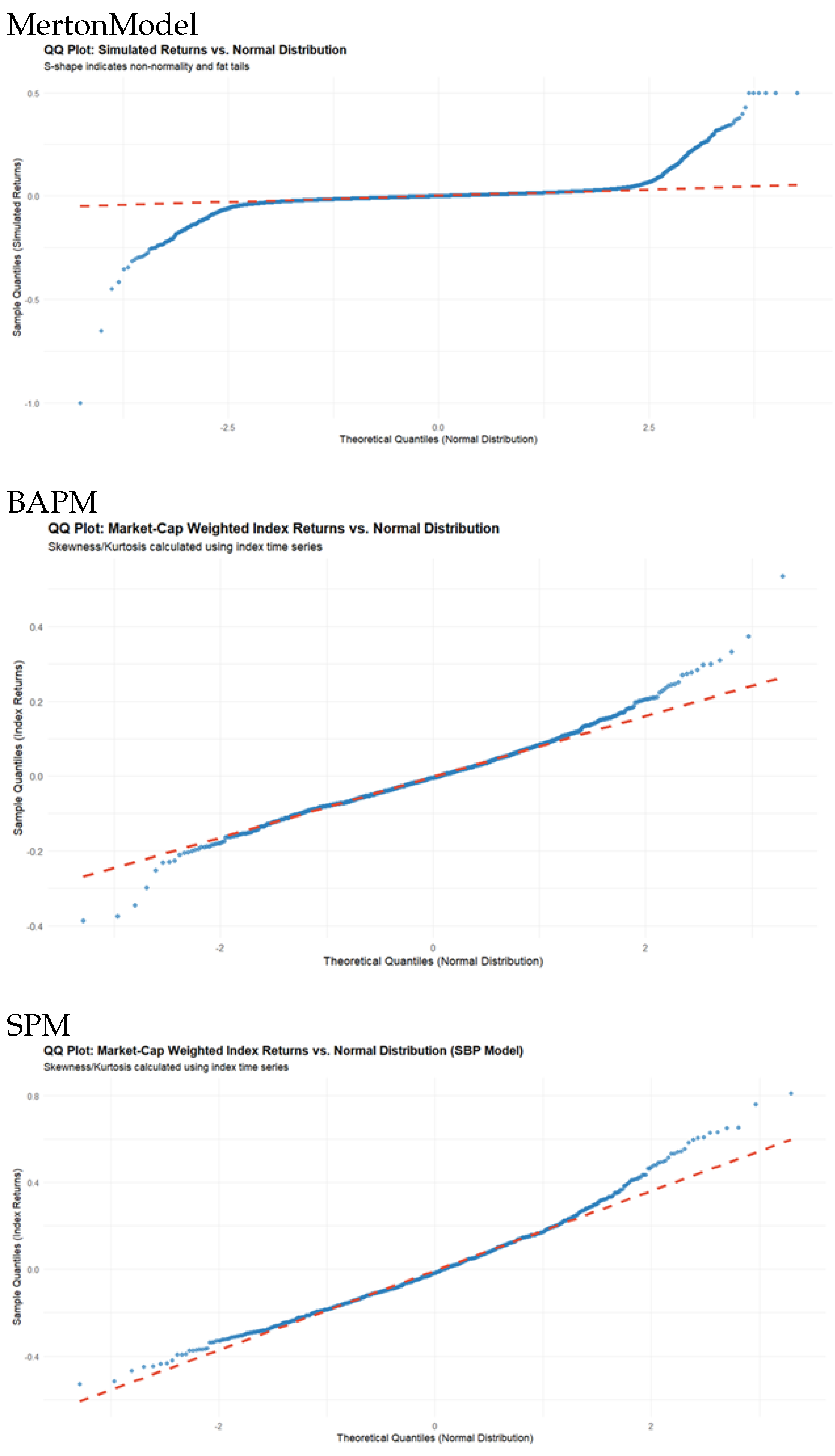
Figure 2.
Plots of the return distributions produced by the Merton Model, BAPM and SPMsimulations
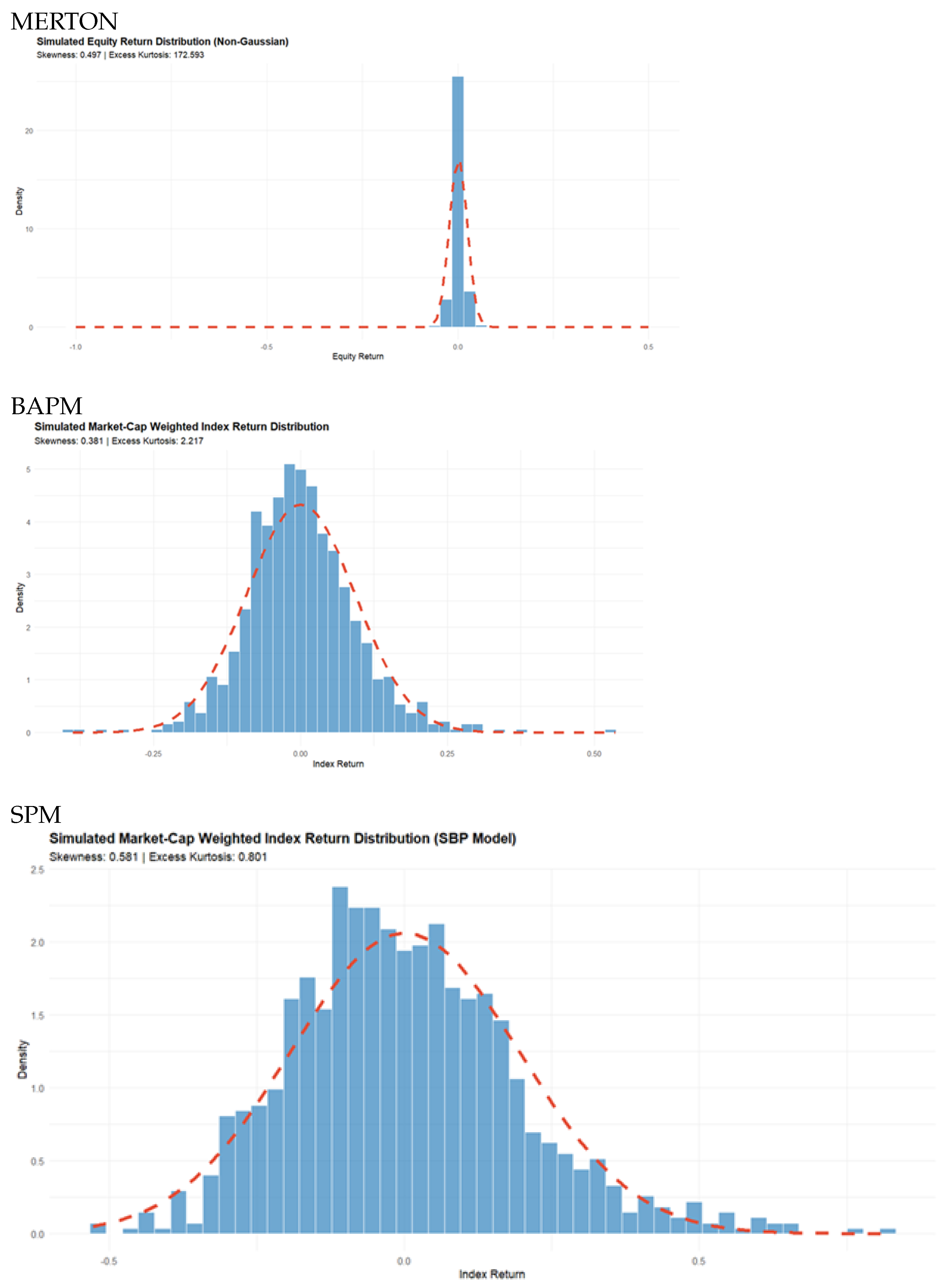
Figure 3.
Plot of Zipf-Mandelbrot Power Law fitted to 3560 US Companies
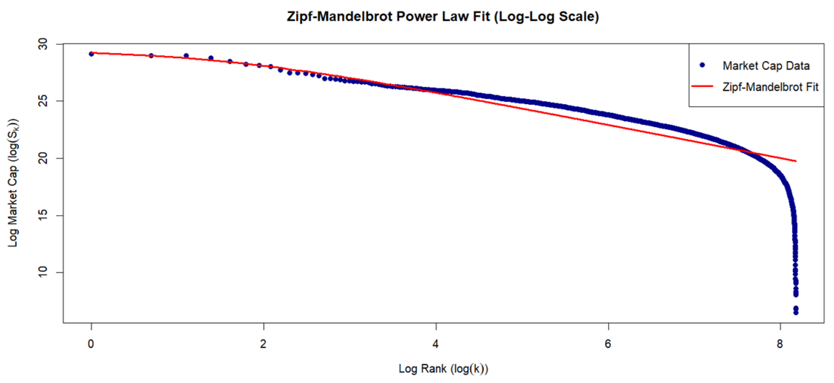
Figure 4.
Zipf-Mandelbrot Power Law fitted to the simulated equity capitalizations generated by the three models.
Figure 4.
Zipf-Mandelbrot Power Law fitted to the simulated equity capitalizations generated by the three models.
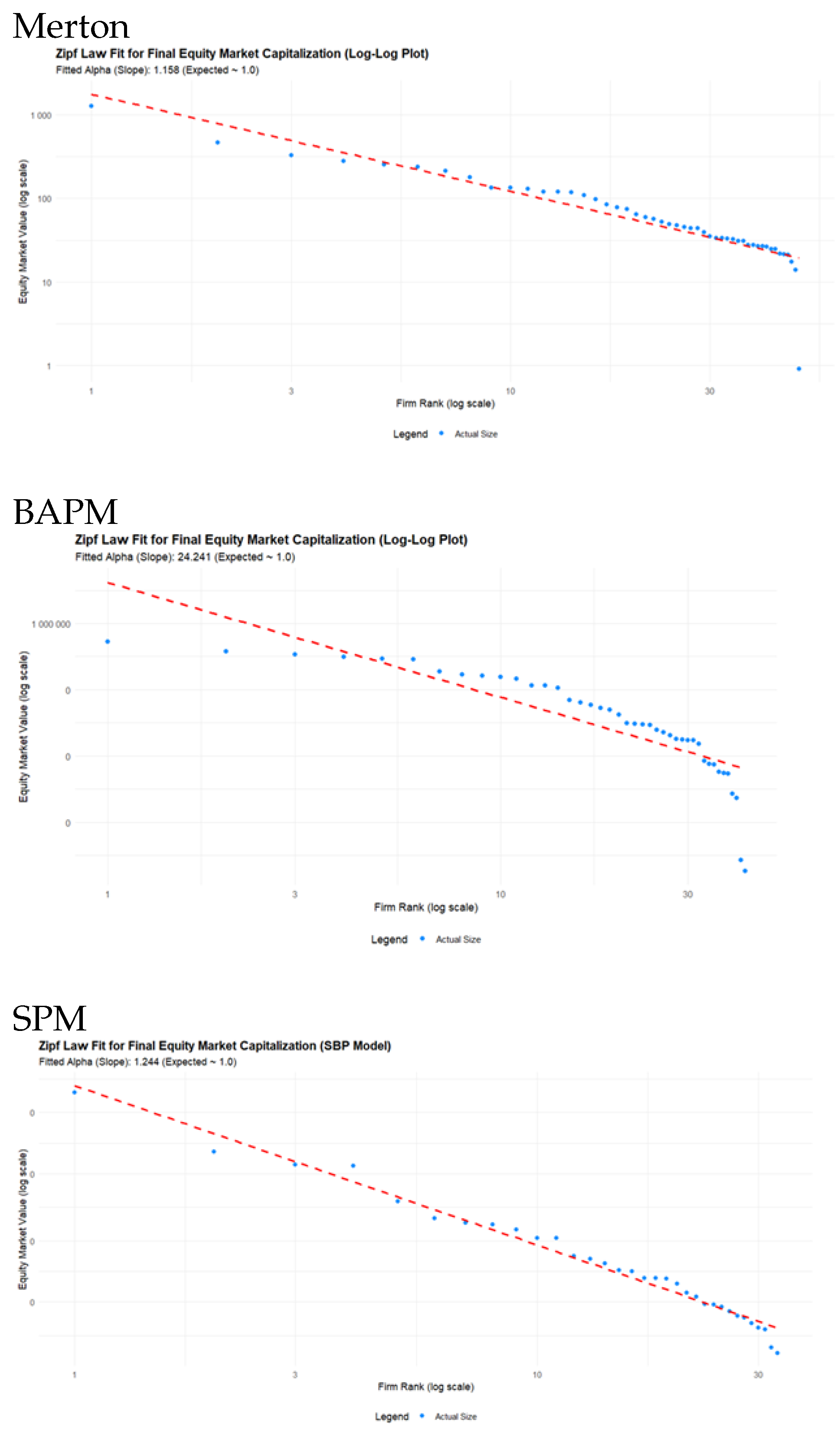
Figure 5.
Leverage effects produced by the three models, Merton, BAPM and SPM

Figure 6.
Heatmap of Systematic Risk Covariance Structure
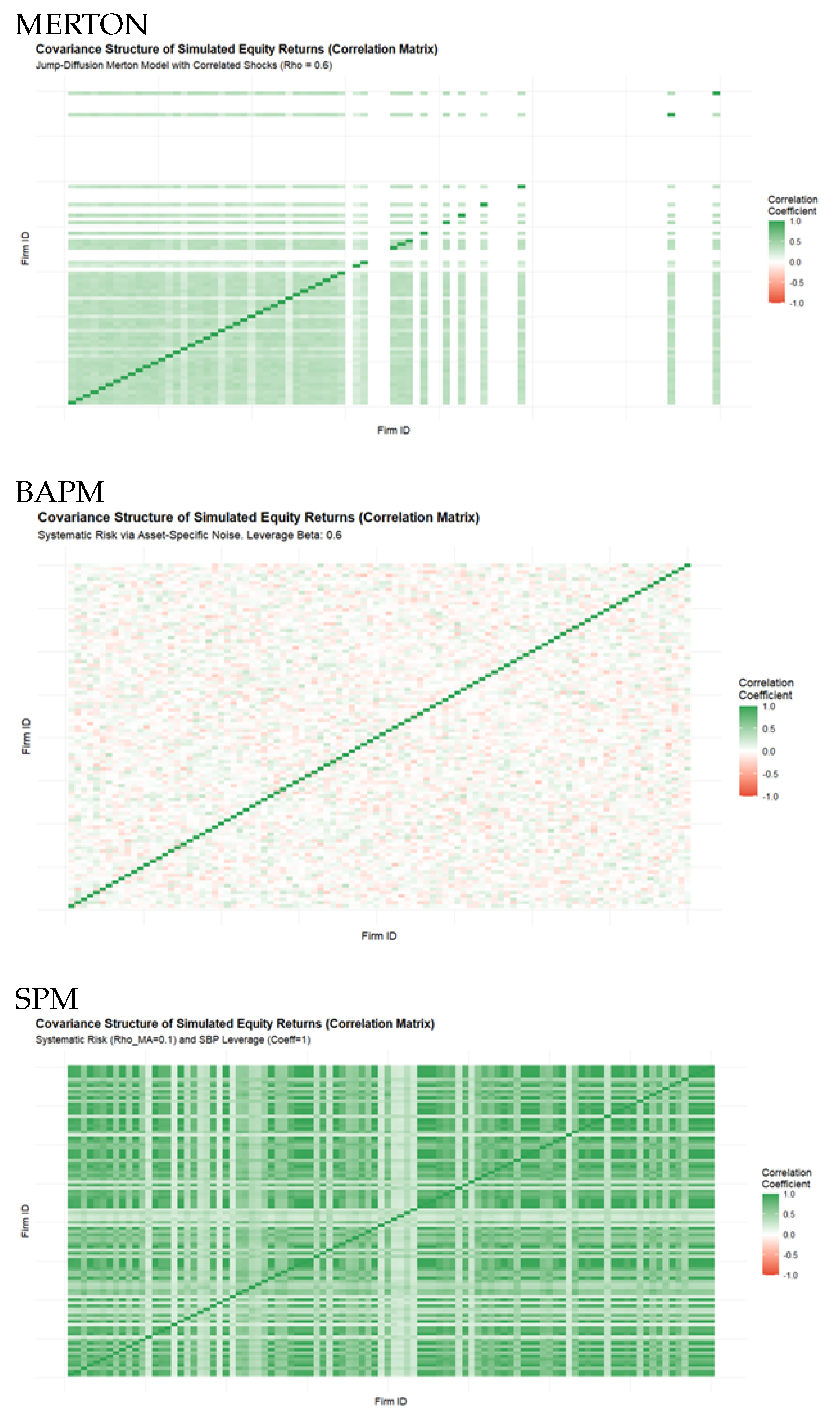
Figure 7.
Long Memory Properties Squared Returns S&P500 Index
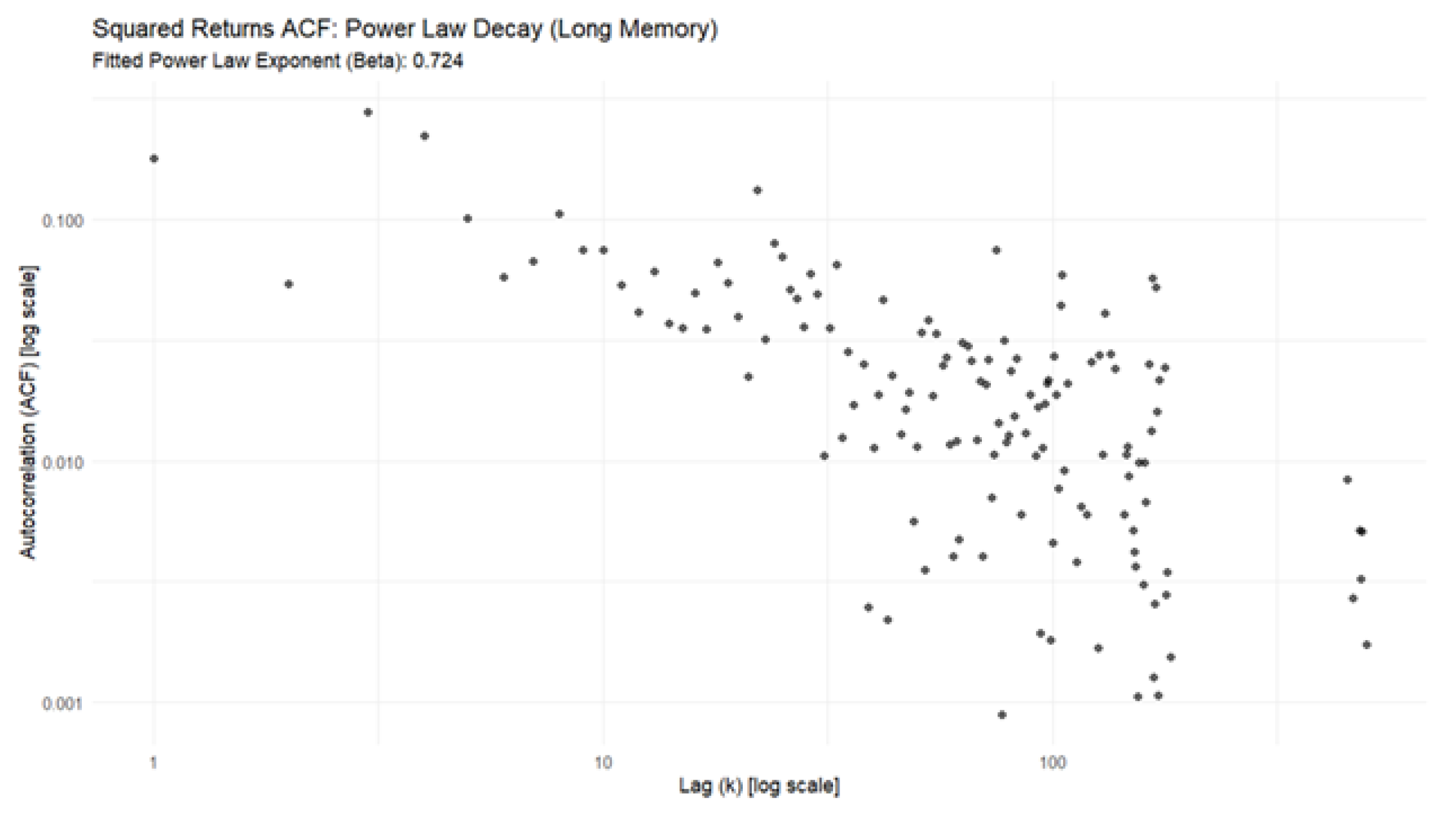
Figure 8.
Long Memory Properties of Squared Returns for the three Simulation Models
Disclaimer/Publisher’s Note: The statements, opinions and data contained in all publications are solely those of the individual author(s) and contributor(s) and not of MDPI and/or the editor(s). MDPI and/or the editor(s) disclaim responsibility for any injury to people or property resulting from any ideas, methods, instructions or products referred to in the content. |
© 2026 by the authors. Licensee MDPI, Basel, Switzerland. This article is an open access article distributed under the terms and conditions of the Creative Commons Attribution (CC BY) license (http://creativecommons.org/licenses/by/4.0/).
Copyright: This open access article is published under a Creative Commons CC BY 4.0 license, which permit the free download, distribution, and reuse, provided that the author and preprint are cited in any reuse.


