
Submitted:
06 January 2026
Posted:
07 January 2026
You are already at the latest version
Abstract
Climate change leads to reservoir management challenges especially in areas with high risk of drought and flood. Traditional reservoir rules curves are inappropriate for addressing variation of reservoir inflow. This study presents an integration framework between GCMs from CMIP6 (ACCESS-CM2, MIROC6, and MPI-ESM1-2-LR) under SSP245 and SSP585 scenarios and WEAP, which is validated in accuracy for reservoir inflow and storage capacity. This integration contributes to Hippopotamus Optimization (HO), a technique used to develop Resilience Reservoir Rule Curve (RRRC) for Ubonrat reservoir during 2024-2055 employing dual-objective function that emphasizes the reduction of water shortage and water excess. The results indicate that RRRC developed by HO is more efficient and suitable than Honey Bee Mating Optimization (HBMO) and existing rule curve. After testing the RRRC with historical inflow and future inflow from three GCMs under SSP245 and SSP585, it can reduce average water shortage and demonstrate outstanding efficiency in water excess management. This potential reflects its adaptability under future variation of hydrological condition. This crucial finding illustrates that the integration framework can develop resilient rule curves under uncertainty. HO integrated with various models can be implemented as an optimal framework and have high potential for reservoir operation planning under climate change. The developed methodology can be implemented in other reservoirs to gather additional factors for sustainable promotion of water resource resilience.
Keywords:
climate change
; reservoir inflow variation
; reservoir rule curves
; hippopotamus optimization algorithm
; resilience water management
1. Introduction
Climate change has a significant impact on hydrological cycle throughout the world especially headwater areas, reservoir inflow, and surface water management. It becomes challenging for reaching the 6th Sustainable Development Goal (SDG6) set by the United Nations, which focuses on sustainable water management and sanitation for all [1,2]. This change also affects evapotranspiration and river streamflow, which leads to another challenge that has never happened before for water resource management and planning. Moreover, uncertainty and variability caused by climate change significantly exert an effect on management policy of water resource, such as water allocation at a reservoir for various activities using reservoir rule curves developed using pervious hydrological data [3,4] together with water allocation by monthly average [5]. However, these traditional ways of reservoir management have their hypotheses that hydrological patterns are constant, but they have been refuted because of climate change and rapid variation of water demand for some activities at downstream. Therefore, agencies being in charge of water resource management have more challenges in policy development to allocate water efficiently for balancing water demand in different activities, such as irrigation, consumption, hydropower generation, and ecosystem conservation. They have to be able to handle the risks of flood and drought, which are obstacles to meet the SDG6, especially the Goals 6.4 on water use efficiency and 6.5 on integrated water management for all level [1].
Water resource management currently depends on more integrated models for future hydrological simulation under climate change situations. This concept is consistent with the Integrated Water Resource Management (IWRM) in the SDG6 that promotes many models, such as Water Evaluation and Planning (WEAP) [6,7], Soil and Water Assessment Tool (SWAT) [8,9], MIKE HYDRO Basin [10,11], and Modeling and Simulation (MODSIM) [12]. These models have been widely used to analyze the effects of climate change on watershed hydrology and water resource management. They are normally driven by General Circulation Models (GCMs) under the Shared Socioeconomic Pathways (SSPs) different from the Coupled Model Intercomparison Project Phase 6 (CMIP6) [13,14] to create future possible hydrological conditions.
At the same time, researchers around the world have developed advanced optimization algorithms integrated with numerically hydrologic or hydraulic models, and they have used data from GCMs to determine an optimal policy for reservoir operation under hydrological changes, such as using Metaheuristic Algorithms (MHAs), which are divided into 3 main types [15]: 1) Evolutionary Algorithms (EAs) consist of Genetic Algorithm (GA), Dynamic Programing (DP), Genetic Programing (GP) [16,17,18]. 2) Swarm Intelligence Algorithms (SIs) consists of Honey-Bee Mating Optimization (HBMO), Ant Colony Optimization (ACO), Firefly Algorithm (FA), Bat Algorithm (BA), Grey Wolf Algorithm (GWA), Particle Swarm Optimization (PSO), Cuckoo Search (CS) [3,19,20,21,22,23,24]. 3) Other MHAs include Harmony Search (HS), Coral Reefs Algorithm, Charged System Search Algorithm [25,26,27]. Nevertheless, the existing algorithms are facing the challenging management of complicated and non-linear system of the reservoir under the climate change, especially either variation of hydrological system in upstream area, or appropriate management of water resource in downstream area [28,29,30].
Over the past decade, Water Evaluation and Planning System (WEAP) is one of the numerical models widely used for analyzing and assessing water management since it has outstanding potential for assessing the impact of climate change on water resource management system [31,32]. Moreover, it can be used for integrating between natural and engineering elements of hydrological system especially for watershed hydrology simulation, reservoir operation, irrigation demand, and water allocation according to priority defined by user [33,34,35]. The model is appropriate for assessing water resource comprehensively by predicting the climate change obtained from GCM to analyze the impact on water yield and water demand [36,37,38,39] in order to develop optimal adaptability [40]. Integrated with optimization technique, WEAP will gain a robust and resilient framework for reservoir operation enhancement.
The strength of WEAP is ability to integrate data from GCMs in the Coupled Model Intercomparison Project Phase 6 (CMIP6) under different Shared Socioeconomic Pathways (SSPs) [41,42]. The integrated studies encourage researchers to develop future hydrological simulation with high reliability. The previous studies have used data from CMIP6 under SSP2-4.5 and SSP5-8.5 scenarios in driving WEAP to get more understanding of the impact of climate change on runoff at major watershed around the world [43,44]. For instance, seasonal precipitation variation of the SSP5-8.5 scenario of Mekong watershed tends to get significantly higher during 2021-2060. Similarly, another Mekong river basin study has revealed that integrating WEAP with the outcome from CMIP6 can be more precise in assessing the risk of water scarcity [45]. In the context of Nile watershed, Ly et al. [46] indicates that CMIP6 can be used efficiently for analyzing the impact on streamflow into a dam. In South Asia, WEAP driven by GCMs can simulate groundwater volume change reliably [47]. In this regard, the efficiency of integration in nested watersheds has been affirmed regarding diverse water use [48], showing the resilience and adaptability in different hydrological system. This integration is counted as important development in improving the precision of future hydrological prediction, which is significant for efficient and sustainable water management policies under climate change [49].
During 2024, Hippopotamus Optimization (HO) is a metaheuristic algorithm of optimization developed and inspired by 3 hippopotamus’ behaviors, including hippopotamuses position update in the river or pond, hippopotamus defense against predators, and hippopotamus escaping from the predator [50]. HO is defined through a triangular model including positioning in a river or pond, defensing against predators, and escaping, and it is designed as a mathematical formula, which is more unique compared to other types of metaheuristic algorithm [51]. In addition, it has the potential to solve problems of complicated engineering design, such as Tension/Compression Spring, Welded Beam, Pressure Vessel [50], Distribution Network Reconfiguration [52] and Power System Stabilizer [53]. According the literature review, nevertheless, application of HO to water resource system development is still limited, particularly in improving reservoir operation rule curves under the climate change; meanwhile, many studies used traditional optimization algorithm with WEAP for water resource management. The algorithm has been limited in complication management and uncertainty of hydrological system under climate change [54], particularly when it has to be integrated with data from CMIP6, which have high resolution and precision at present [41,47].
The impacts of climate change on hydrological system and limited traditional reservoir operation strategies become an important research gap and need to have a resilient management policy that is aligned with the goal 6.4 of SDG emphasizing the improvement of water consumption efficiency and sustainable water security [55]. This study can meet this essential need by integrating climate change forecast, hydrological simulation, and advanced optimization technique to develop reservoir operation resilience. The selected case study is Ubolrat Reservoir, which is the largest multipurpose reservoir in northeastern Thailand for hydropower generation, agriculture, and consumption. Currently, this reservoir is affected by climate change and water demand variation in downstream area [56]. For this reason, this study has been conducted to understand its previous, current, and future condition with 3 main objectives: 1) to simulate inflow into the Ubolrat Reservoir and allocate future water in downstream for the reservoir using WEAP driven through climate condition forecast from GCMs and CMIP6 under SSP245 and SSP585 scenarios during 2024 – 2055; 2) to enhance the reservoir operation rule curves that adapt to climate condition and provide optimal water allocation using optimization algorithm; and 3) to assess efficiency of reservoir operation rule curves developed to compare to the existing policy of reservoir operation and optimal reservoir operation rule curves developed through other techniques previously studied.
The research is expected to be part of promoting water resource management adaptable to climate circumstance that provides optimal innovation, method, and guideline for those who are in charge of reservoir, irrigation, and hydropower generation management, as well as reservoir stakeholders dependent on the model of Ubolrat Reservoir case study. The developed approach presents the transferable frameworks to enhance resilience under climate change for global reservoir system. It also promotes sustainable water management under higher level of hydrological uncertainty to respond directly to the goal of SDG6 to ensure sustainable provision of water and sanitation for all and to meet the goal of SDG13 to take urgent action to overcome climate change and its impacts.
2. Materials and Methods
2.1. Study Area
Ubolrat Reservoir is located in northeastern region of Thailand between 101°30'-103°00' E longitude and 16°30'-17°20' N latitude as shown in Figure 1. Hydrological characteristic of the watershed area can be classified into 2 main parts. First, upstream area consists of 8 sub-watersheds: Upper Phong Part 1, Part 2, Part 3, Puai, Lam Phaniang, Prom, Choen Part 1, and Part 2 sub-watersheds with approximately areas of 12,053.2 square kilometers (sq.km), where inflow flows into the Ubolrat Reservoir. Second, downstream area consists of Lower Phong Part 1, Part 2, and Huai Sai Bat sub-watersheds with approximately areas of 3,003.4 sq.km. Flow direct is from western and northern upland areas flowing toward the east and south. The mean annual precipitation is 1,100-1,400 mm. The reservoir structure is earth-fill dam with clay core and has gross storage capacity of 2,263 million cubic meters (MCM). Its mean annual inflow is 1,750 MCM with installed capacity of 55 million kWh/year. Its mission consists of 4 major missions: 1) hydropower generation, 2) irrigation water supply, 3) flood mitigation, and 4) eco-tourism.
2.2. Spatial Data Collection
Collected data are composed of two parts: WEAP and reservoir operation rule curve developments. 1) WEAP development data include meteorology, daily precipitation of 19 stations, monthly average temperature of 2 stations located at weather stations in Nong Bua Lamphu and Khon Kaen Provinces during 2000 – 2023, and physical data of watershed such as digital elevation model (DEM), land use, and soil group maps, as shown in Figure 2. 2) Data on reservoir operation rule curve development by HO technique consist of Ubolrat Reservoir inflow during 2000 – 2023, evaporation, reservoir storage capacity, allocated water supply from downstream (for consumption, agriculture, industry, ecosystem conservation, etc.). Both data are presented in Table 1.
2.3. General Circulation Models and Bias Correction
Future climate change analysis is a main consideration of future changes in precipitation and temperature [29]. They are then used for analyzing future inflow volume and water balance by using WEAP. In analysis process, it starts from retrieving future climate data from the GCMs under the CMIP6 for 3 models including ACCESS-CM2, MIROC6, and MPI-ESM1-2-LR. The retrieved data were used for analyzing the changes of precipitation, maximum, and minimum temperatures. For future scenarios, SSP245 and SSP585 are analyzed as presented in Table 2.
In bias correction from GCMs, data from the NASA Earth Exchange Global Daily Downscaled Projections (NEX-GDDP) [57], a database in WEAP, are employed. NEX-GDDP is a downscale database for GCMs and includes downscale projection from ScenarioMIP that is produced and disseminated daily through Earth System Grid Federation (ESGF) [58]. This data set is provided to prepare a set of climate change projections with high resolution that is bias-corrected and applied to the assessment of impact of climate change on sensitive processes of each topographic condition [59].

Table 2.
GCMs for future climate change analysis.
| No. | Model | Resolution (km) | Institute |
|---|---|---|---|
| 1 | ACCESS-CM2 | 250 × 250 | Commonwealth Scientific and Industrial Research Organization, Australia [60] |
| 2 | MIROC6 | 250 × 250 | Model for Interdisciplinary Research on Climate, Japan [61] |
| 3 | MPI-ESM1-2-LR | 250 × 250 | Max Planck Institute for Meteorology, Germany [62] |
2.4. Reservoir Inflow Analysis Using WEAP
2.4.1. Principle of WEAP
Water Evaluation and Planning (WEAP) is a tool for water resource planning and management developed by Stockholm Environment Institute using Soil Moisture Method, which is a lumped model to analyze two-bucket system. The upper represents soil moisture absorbed by plant roots while the lower represents deep groundwater that can be baseflow absorbing into the groundwater layer [7,63]. The strength of WEAP is ability to simulate all hydrological process naturally and integrate water management in the system [32,48]. It is appropriate for assessing the impacts of climate change and land use as well as analyzing situations for sustainable planning of water resource management. The basic equation of WEAP for calculating water balance of the upper layer can be seen in Equation (1):
where Rdj is water storage capacity of soil, z1,j is soil moisture ratio at upper layer, Pe is precipitation, PET is reference evapotranspiration, Kc,j is crop coefficient, RRFj is runoff resistance factors, ks,j is saturated water conductivity, and fi is water partition coefficient horizontally and vertically.
Streamflow calculation in WEAP is composed of 3 main elements.
- Surface runoff is calculated from total runoff using Equation (2):
- Interflow can be calculated by using Equation (3):
- Baseflow is calculated using Equation (4):
The total runoff flowing out of a watershed area is the sum of 3 elements from Equation (2) – (4), where WEAP calculates water balance for land use type and aggregates the results that can lead to actual evapotranspiration using Equation (5):
where ET is actual evapotranspiration (mm per unit time), ET0 is reference evapotranspiration calculated based on weather condition through Penman-Monteith (mm per unit time), Kc is crop coefficient dependent on crop types and growth stage (unitless), and z1 is soil moisture ratio at upper layer compared to maximum capacity from 0-1 (unitless).
Data are integrated with WEAP through division of watershed area into subunits based on land use types [7,38]. Each unit has specific parameters representing the area characteristics. Data on monthly climate consist of precipitation, temperature, relative humidity, and wind speed, which are used for calculating ET0 using Penman-Monteith approach. Data on ground cover are used for specifying Kc for agriculture, forest, grassland, and urban areas, as well as specifying RRF that controls the surface runoff. Data on soil types are employed to identify water hold capacity (SWC, DWC), and saturated water conductivity (Ks), and water partition coefficient (f) that affects baseflow. Watershed boundary is used for identifying calculation area and confluence point. WEAP calculates water balance according to land use type, and calculate product sum using area proportion to gain the total of streamflow at watershed outlet [48,64]. This data integration can help WEAP to simulate the impacts of climate change or land use per streamflow efficiently.
2.4.2. Model Calibration and Validation
WEAP calibration and validation are comparison between inflow of the Ubolrat Reservoir and storage volume obtained from the model and 24-year monthly measurement (2000 - 2023) separated into 12-year calibration (2000 - 2011) and 12-years validation (2012 - 2023). The assessment uses statistical values: R2, NSE, RSR, and PBIAS, which are used for checking reliability of the model, as shown in Equations (6) – (9):
where Oi is the measured inflow and storage volume, Ō is an average of measured inflow and storage volume, Pi is inflow and storage volume calculated by the model, is an average of inflow and storage volume calculated by the model, and i is data order.
2.5. Hippopotamus Optimization Connected with Reservoir Simulation Model for Optimal Resilience Rule Curves
Hippopotamus Optimization (HO) is an optimization algorithm inspired by 3 hippopotamus’ behaviors: (1) river and pond exploration, (2) defensing against predators, and (3) escaping from predators. The algorithm functions start from creating random initial population according to Equation (10). Each hippopotamus is substituted a possible result for parameters of Resilience Reservoir Rule Curve (RRRC):
where Xi,j is hippopotamus position i in dimension j (i = 1,2, ……, Npop; j = 1,2,….., nvar) that parameter of rule curves is substituted by nvar = 24 (12 values for monthly upper rule curve and 12 values for monthly lower rule curve), r is random number in the interval [0,1], and are lower and upper bounds of variables j according to the reservoir constrains, and Npop is population size.
In applying HO to optimize RRRC, dual-objective function is designed to assess the efficiency of system comprehensively by analyzing both drought and flood risks. The objective function is defined as Equation (11):
where F is dual fitness scores, w1 and w2 are weight coefficient which normally specifying w1 = w2 = 0.5 for equal importance, Shortagey is total water shortage volumes in year ν (MCM), Spilly is total overflow in year ν (MCM), and N is total number of years during simulation.
Optimization of HO Algorithm is divided into 3 important phases. Each phase specifically simulates hippopotamus’s behaviors in different situations. Phases 1 and 2 focus on comprehensive exploration of solution space to avoid being stuck at the specific lowest spot as Equation (12) and (13). Phase 3 emphasizes exploitation to improve the solution as Equation (14). Switching among these three phases equally can allow the algorithm to gain resilience rule curves.
Phase 1: Exploration
where xbest,j is the position of leading hippopotamus, xrand,j is the position of randomized hippopotamus, r1 is random number in the interval [-1,1], and is temperature parameter reduced dependent on time.
Phase 2: Defense
where is the position of predators, is distance, Lj is Levy flight vector, and M are defense factors in the interval [0,1].
Phase 3: Exploitation
where r3 is random number in the interval [-1,1] and t is current iteration.
Regarding each iteration and evaluation using a reservoir model, each hippopotamus is defined to be qualified one of the three phases through random sampling. A new position is then validated under the boundary as Equation (15).
Next, a reservoir simulation model [65,66] is used to consider the outflow based on the standard operating rule using Equation (16):
where Rν,τ is volume of water discharged from reservoir in year ν and month τ (MCM) (τ = 1 to 12 represents January to December), Dν,τ is water demand in month τ (MCM), xτ is water volume of lower rule curve in month τ (MCM), yτ is water volume of upper rule curve in month τ (MCM), and Wτ is water storage volume in reservoir calculated from simple water balance (MCM) as Equation (17) [66]:
where Sν,τ is storage volume in the end of month τ, Qν,τ is inflow of reservoir, and Eτ is water loss from evaporation.
When completing algorithm, hippopotamus parameters will be transferred into optimal RRRC parameters for 24 values of rule curve in all months (12 upper rule curves and 12 lower rule curves). The developed reservoir rule curves are expected to be used for reservoir management equally between reducing water scarcity risk and discharging excess water. HO functions are connected to the reservoir simulation model as illustrated in Figure 3.
Furthermore, this study developed the RRRC using Honey-bee Mating Optimization (HBMO) technique to compare its performance with HO and existing rule curves of Ubolrat Reservoir. HBMO is an optimization technique inspired by bee mating behavior, encompassing key processes such as queen bee flight, bee incubation, and worker bee quality improvement. The RRRC development process using HBMO employs the same objective functions and reservoir model connections as HO, following the approach of Songsaengrit and Kangrang in 2022 [3].
3. Results and Discussions
3.1. Climate Change Analysis
3.1.1. Future Precipitation
In analyzing future change in monthly average precipitation for the Ubolrat Reservoir watershed areas using Thiessen Polygon of 3 GCMs compared with the past to the present (2000 – 2023: Baseline (BL)) as presented in Figure 4 (a) - (b), future monthly precipitation distribution of both SSP245 and SSP585 scenarios has the same pattern as the past to the present, which is high precipitation in rainy season but low in dry season. In case of future period from 2024 - 2055, a change can be found in both scenarios that is precipitation in January close to the past. However, the precipitation during February – May significantly increases, especially in May increasing from 6 mm to 160.6 mm for SSP245 and 158.8 mm for SSP585. In June, the precipitation is comparable to the past, but it becomes higher in July and August. At the end of the rainy season, the precipitation in September is close to the past; however, it significantly decreases during October – December compared with the BL.
In Figure 4 (a) - (b) and Table 3, the result of analyzing annual precipitation indicates that from the BL, the average annual precipitation is 1,188.4 mm. In the future range (2024 – 2055), the annual precipitation of SSP585 tends to be slightly higher than SSP245. In case of SSP245, the precipitation increases 12.5% that leads to the increase of average precipitation of 1,336.8 mm per year. At the same time, it increases 13.4% for SSP585 that leads to average precipitation of 1,347.6 mm per year. As a result, it can be described the linear transformation of precipitation that SSP245 has its trendline y = 2.9538x + 4715.7 and R2 = 0.0352 while SSP585 shows y = 3.3883x + 5588.8 and R2 = 0.043. This can indicate that precipitation of SSP585 is higher than SSP245. Moreover, from analyzing annual maximum and minimum of all 3 GCMs, SSP245 shows its average precipitation between 1,189.3 – 1,482.2 mm per year, which has narrow range compared with SSP585, which has average precipitation between 1,144.5 – 1,567.5 mm per year. It means that SSP585 has higher uncertainty and critical change than SSP245.
3.1.2. Future Temperatures
In the analysis result of monthly average of future temperature from 3 GCMs compared to a period from the BL is presented in Figure 4 (c) – (d). The future period during 2024 – 2055 demonstrates average temperature of every month higher than the period from the past to the present in both SSP245 and SSP585. This increase in temperature is constant the whole year – the highest increase can be seen during March – April. When considering the maximum and minimum of 3 GCMs, SSP245 and SSP585 have comparable values. Nevertheless, SSP245 has slightly wider range than SSP585, particularly in summer (March - May), which indicates higher variation of temperature.
In calculating annual average temperature as shown in Figure 4 (c) - (d) and Table 4, the range BL has average temperature of 27.7 °C and tends to get higher in the future. It is slightly higher in SSP585 than in SSP245, where average temperature for SSP245 increases 1.0 °C, so it becomes 28.7 °C increase while the average temperature increase for SSP585 is 1.1°C, so its increased temperature becomes 28.9 °C on average. In addition, the result of analyzing annual maximum and minimum of the 3 GCMs indicates that SSP245 has annual average temperature between 28.0 °C and 29.4 °C, which is wider by range than SSP585 that has temperature between 28.1 °C and 29.1 °C. It means that SSP245 has higher variation than SSP585.
According to the result of change trend (Figure 4 (c) - (d)), both scenarios show the increase in temperature over the course of the study. SSP245 has its trendline equation y = 0.0321x + 36.885 and R2 = 0.5794 while the trendline equation of SSP585 is y = 0.0381x + 49.967 and R2 = 0.6409. It indicates that SSP585 shows higher rate of temperature and stronger linear correlation than SSP245. This is consistent with a prediction of significantly greater increase in temperature for SSP585 due to high emissions of the greenhouse gas.
3.2. Simulation of Future Inflow into Reservoir by WEAP
3.2.1. Sensitivity Analysis of Parameters
During calibration process, there are adjusted 7 parameters that affect the inflow and are widely used by many studies [67], including Crop coefficient (Kc), Soil water capacity (SWC, mm), Deep water capacity (DWC, mm), Runoff resistance factor (RRF), Root zone conductivity (RZC, mm per month), Deep conductivity (DC, mm per month), and Preferred flow direction (PFD). The adjustment has to be performed until gaining R2, NSE, RSR, and PBIAS, which can demonstrate relationships between calculation results and optimal measurement values based on international standard as presented in Table 5 [68].
The result of parameter adjustment can be classified into 2 groups according to land use features. The first group consists of Kc, SWC, and RRF, which represent a significant variety based on land use type, where Kc ranges from 0.40 for urban area to 1.04 for forest area inferring from 50 to 1,000 mm, and RRF ranges from 0.2 to 4.0. This difference reflects a hydrological process at the surface, especially water partition among plant evapotranspiration, soil water capacity, and runoff, which have close relationship to surface properties and crops. In contrast, the second group includes DWC, RZC, DC, and PFD. These are parameters for land use type, where DWC is specified at 1,000 mm, RZC at 20 mm, DC at 20 mm, and PFD at 0.15 mm. The fact that the parameters invariant with respect to the land use type can indicate subsoil and groundwater processes such as infiltration, baseflow, and groundwater discharge are physical properties of soil that are not dependent on plant types and general land use. This result is in line with hydrological principles explaining that soil and its structure are factors identifying water behaviors in soil systems [7]. The optimal adjustment for the parameters of the study area is presented in Table 6.
3.2.2. Efficiency and Precision of WEAP
Reliability evaluation of WEAP uses data on reservoir inflow and storage volume calculated by the model compared to data obtained from monthly measurement stations divided into calibration period from 2000 - 2011 (12 years) and validation period from 2012 - 2023 (12 years). The evaluation result shows statistical indices as shown in Table 7. In calibration during 2000 – 2011, the model reveals outstanding efficiency in reservoir inflow simulation with R2 = 0.84, NSE = 0.82, RSR = 0.43, and PBIAS = -5.20%. However, an ability of the model to simulate storage volume during the same period is slightly lower; R2 = 0.66, NSE = 0.66, RSR = 0.58, and PBIAS = -0.66%. This difference is probably caused by complex simulation of storage volume due to accumulation of all water balance elements over the course of the study [69], as well as parameter adjustment mentioned in 3.2.1 explaining hydrological processes sufficiently [48,64,70]. On the whole, the model, evaluated and validated by statistical indices in terms of reservoir inflow and storage volume, is at high level and acceptable based on the criteria in Table 5. In addition, it can be validated by compatibility of both temporal data during 2000 – 2023 as shown in Figure 5 (a) and (b). This outcome reflects the efficiency of WEAP to simulate scenarios related to the reservoir, and it is applicable to simulation for the Ubolrat Reservoir under future condition of climate change.
3.2.3. Future Inflow of Ubolrat Reservoir
The simulation result of future Ubolrat Reservoir inflow by WEAP (through calibration and validation) under climate change using data inputted from 3 future GCMs compared to past-present period during 2000 – 2023 is illustrated in Table 8 and Figure 7, Figure 8 and Figure 9. According to analyzing the annual average of Ubolrat Reservoir inflow (Table 8), baseline during 2000 – 2023 has the average inflow of 2,811.0 MCM, and future period during 2024 – 2055 has an increasing tendency of inflow in all models and scenarios. The ACCESS-CM2 under SSP245 and SSP585 scenarios shows that the inflow increases to 3,401.5 MCM (21.0%) and 3,326.3 MCM (18.3%) respectively. The MIROC6 demonstrates that the inflow increases 3,726.7 MCM (32.6%) and 3,860.0 MCM (37.3%) respectively. Meanwhile, the MPI-ESM1-2-LR also shows that the inflow increases to 3,501.2 MCM (24.5%) and 3,565.1 MCM (26.8%) respectively. Based on these 3 models, the future reservoir inflow increases to 3,543.1 MCM (26.0%) under SSP245 and 3,583.8 MCM (27.5%) under SSP585. It means that climate change significantly influences an increase in Ubolrat reservoir inflow that affects water storage and allocation for many purposes in the future.
Figure 6.
Average monthly inflow of Ubolrat Reservoir for each scenario.
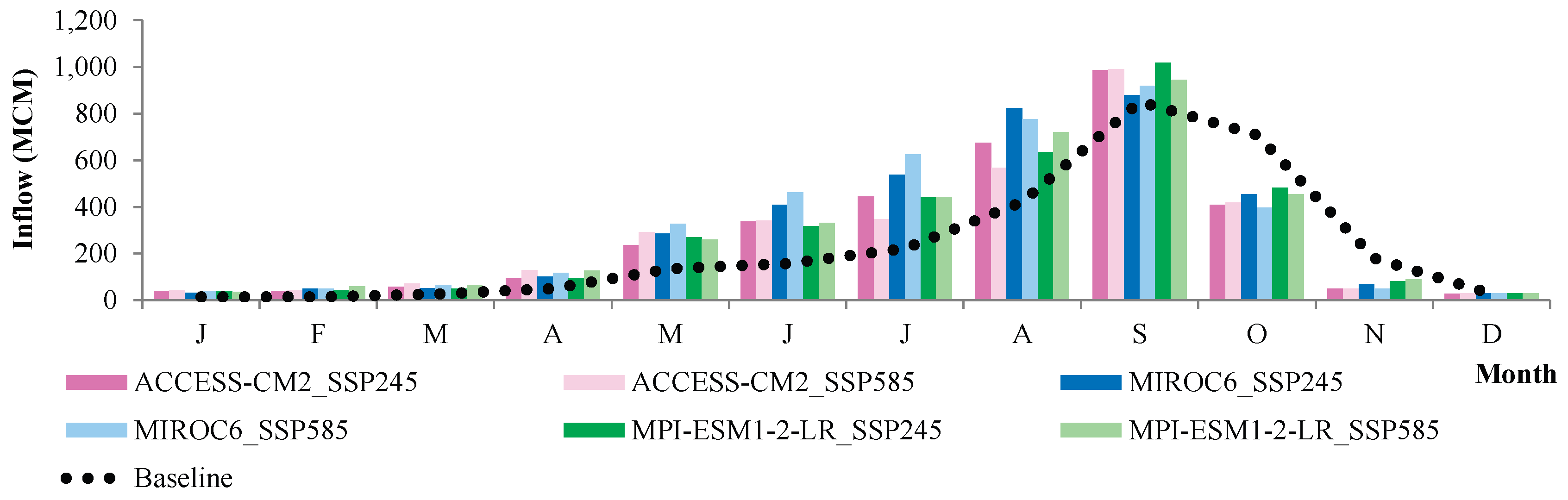
Figure 7.
Monthly inflow of Ubolrat Reservoir during 2000-2055.
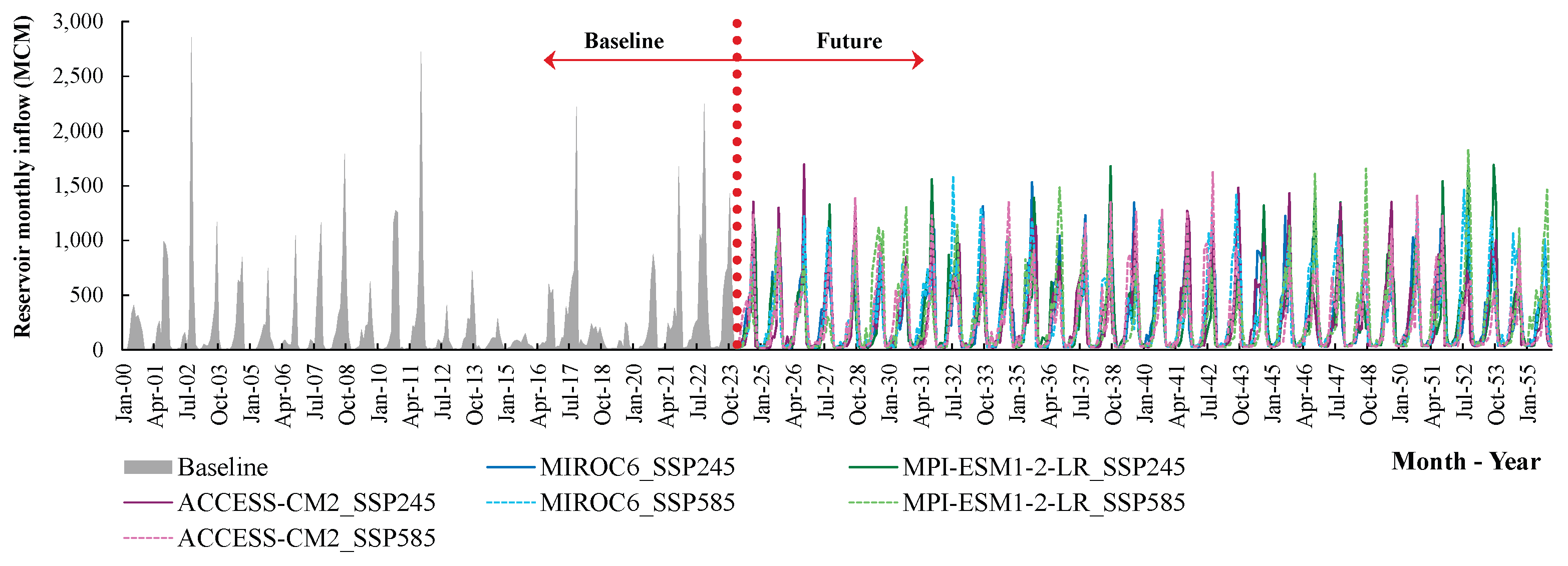
Figure 8.
Annual inflow of Ubolrat Reservoir during 2000-2055.
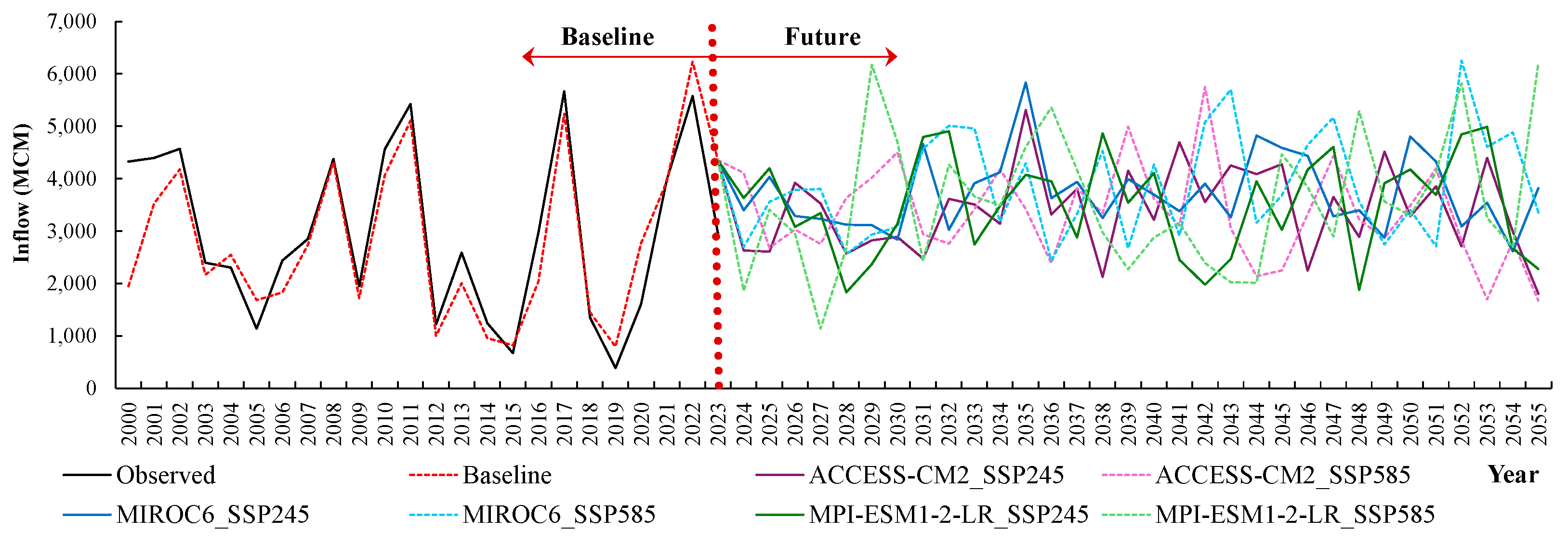
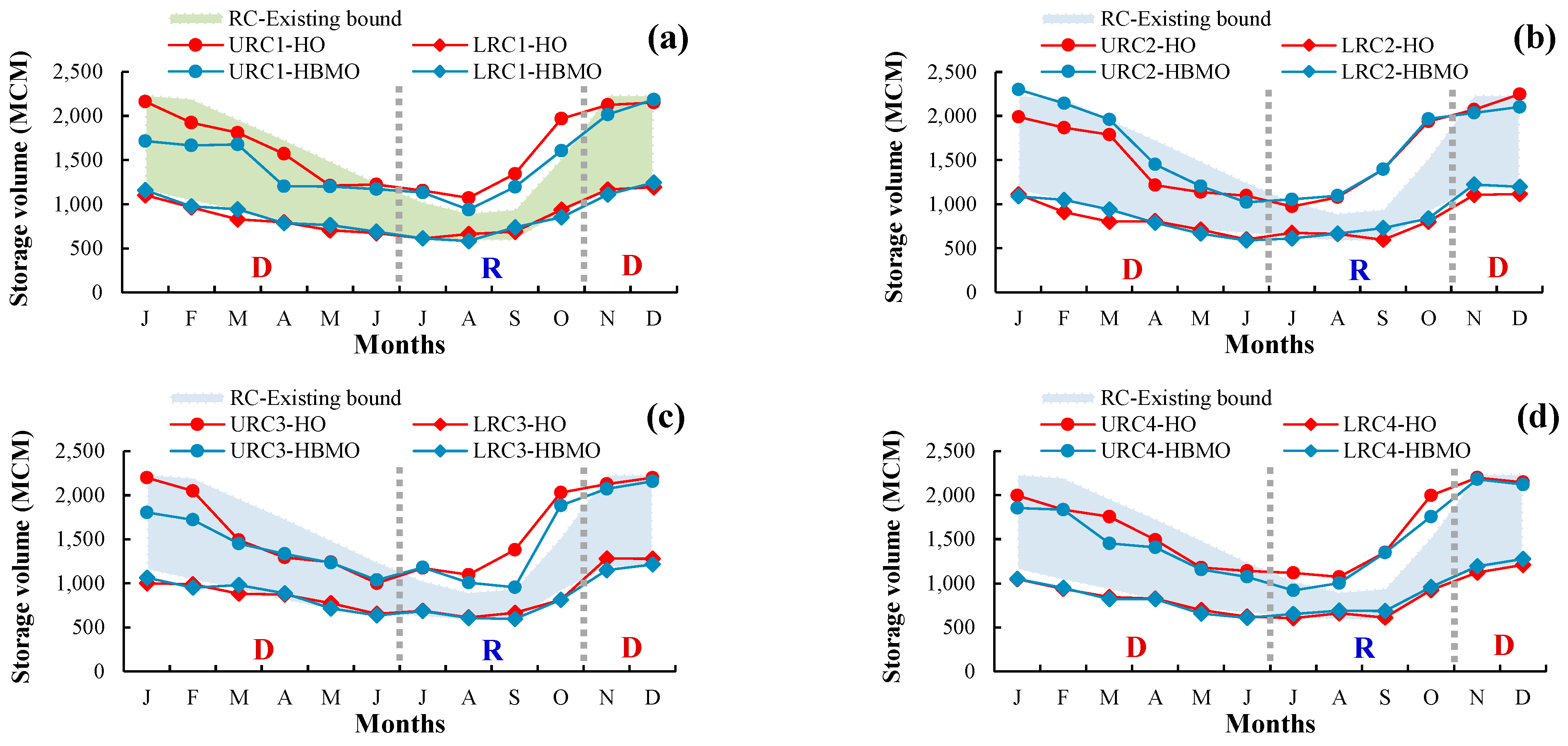
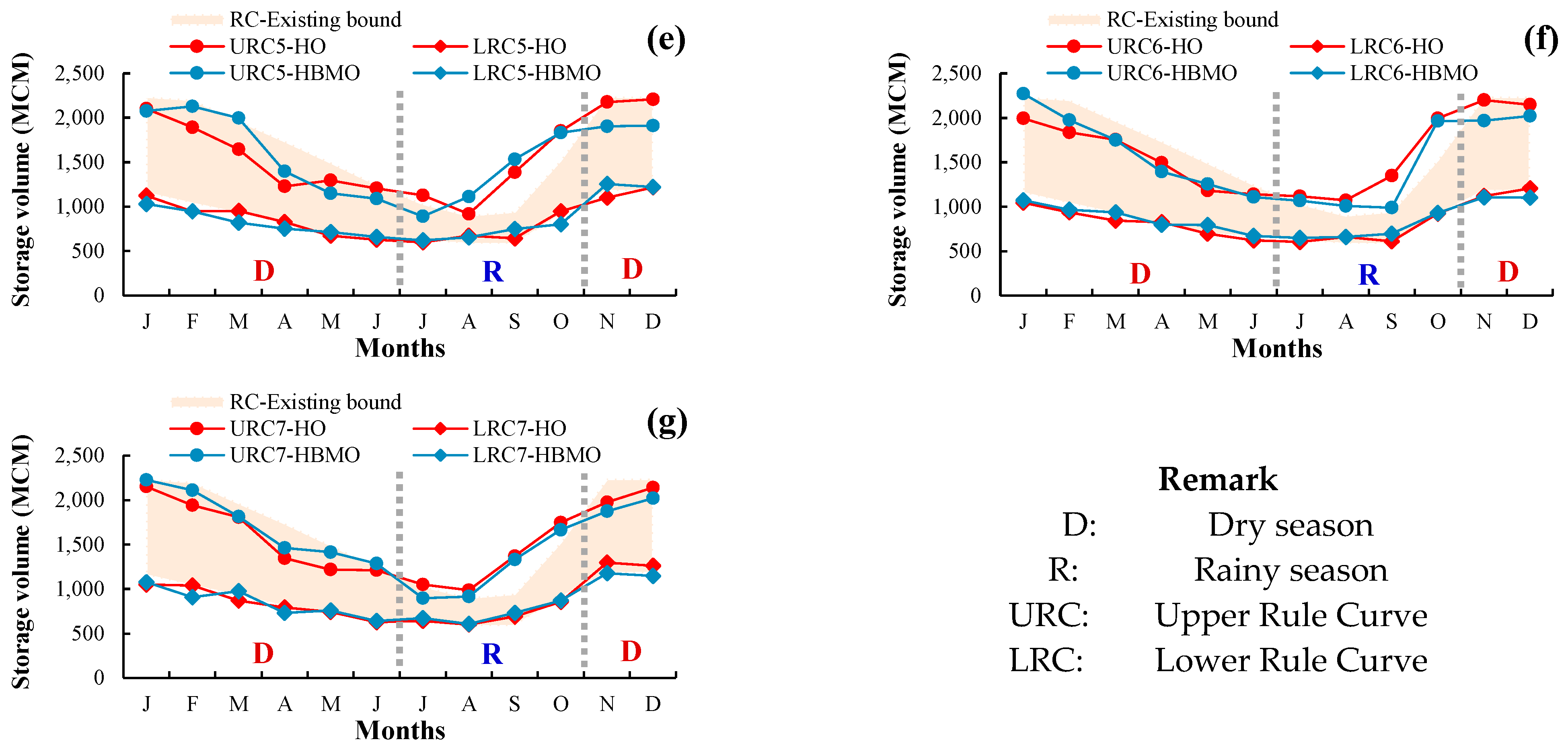
Figure 9.
Resilience reservoir rule curves developed form HO and HBMO using the historic inflow, future inflow from 3 GCMs under SSP245 and SSP585 scenarios compared with the existing rule curves bounds: (a) historic inflow, (b) ACCESS-CM2_SSP245, (c) MIROC6_SSP245, (d) MPI-ESM1-2-LR_SSP245, (e) ACCESS-CM2_SSP585, (f) MIROC6_SSP585, (g) MPI-ESM1-2-LR_SSP585.
The analysis of monthly average of reservoir inflow is presented in Figure 6. This indicates that 3 GCMs show the inflow higher than baseline during January – September, particularly a significant increase in the rainy season (May - September). However, in October and November, the inflow is lower than the past – present period. The highest inflow is in September, and the future reservoir inflow will increase from 851.5 MCM to 951.7 - 1,018.9 MCM dependent on a selected model or scenario. In comparing among GCMs, the MIROC6 has the highest reservoir inflow, especially at the beginning until mid-rainy season (May - August), followed by the MPI-ESM1-2-LR and the ACCESS-CM2 respectively. During dry season (November - April) all 3 models show highly similar results but still higher than past – present period.
The simulation result of monthly Ubolrat Reservoir inflow during 2000 – 2055 is shown in Figure 7. During baseline, an average of monthly inflow is 234.25 MCM – the maximum = 2,853.60 MCM in September 2002 and minimum = 4.40 MCM in January 2001. According to future prediction by 3 GCMs under SSP245 and SSP585, monthly average inflow increases to 296.9 MCM (+26.8%) – the maximum = 1,829.6 MCM in September 2025 reported by MPI-ESM1-2-LR_SSP585 and the minimum = 16.2 MCM in January reported by the same model. These data illustrate that monthly variation is significantly different among the seasons although overall average increases. Figure 8 presents that the baseline shows average annual inflow of 2,810.97 MCM - the maximum = 6,230.40 MCM per year in 2022 and the minimum = 799.40 MCM per year in 2019, which means that the variation is high (Coefficient of Variation = 55.1%). On the contrary, the average of future period increases to 3,563.47 MCM per year (+26.8%), and variation range is between 1,137.60 and 6,252.90 MCM per year – the maximum is in 2052 reported by MIROC6_SSP585 and the minimum is in 2027 reported by MPI-ESM1-2-LR_SSP585. This result indicates that climate change not only leads to an increase of inflow but also affects variation range and distribution. As a result, reservoir management strategies should be improved to be more flexible, efficient, and suitable for various situations [71].
3.3. Development of Resilience Reservoir Operation Rule Curves
The developed RRRC using HO and HBMO based on inflow data set of seven scenarios are hydrologically consistent with each situation. All rule curves have a clear annual cycle – minimum storage capacity from June to July before the start of the rainy season and maximum storage capacity from October to November following the end of the rainy season as shown in Figure 9 (a) - (g).
3.3.1. Upper Rule Curve for Rainy Season
Upper Rule Curve (URC) plays a key role in specifying allowable maximum storage capacity in the rainy season (July - October) to control overflow and prevent flood. The result of RRRC development shows that the rule curves developed by HO and HBMO increase continually from July and reach the maximum during September – October, where inflow becomes the highest. For the historical data (Figure 9 (a)), URC1-HO has an increase of storage capacity from approximately 1,224 MCM in July to approximately 1,971 MCM in October while URC1-HBMO has approximately 1,169-2,016 MCM in the same period. Compared with URC-Existing, URC1-HO and URC1-HBMO are clearly higher than the exiting curve during September – October, approximately 42% higher in September (1,344 compared with 946 MCM) and approximately 29% higher in October (1,971 compared with 1,527 MCM). It can indicate that the developed curve allows to store more water during late rainy season for reserving water for the upcoming dry season.
The future situations under SSP245 from MIROC6 (Figure 9 (c)) show the highest URC; URC3-HO has approximately 1,000-2,030 MCM in the rainy season that is 16% higher in September and 33% higher in October. This complies with the prediction of higher inflow in this model. Meanwhile, URC2-HO from ACCESS-CM2 (Figure 9 (b)) and URC4-HO from MPI-ESM1-2-LR (Figure 9 (d)) show approximately 27-31% higher than the existing curve in October under SSP585 that has higher variation. URC6-HO from MIROC6 (Figure 9 (f)) is also higher than the existing curve during the rainy season; 43% higher in September and 31% higher in October. On the other hand, URC5-HO from ACCESS-CM2 (Figure 9 (e)) show only 21% higher level than the existing curve in October, and URC7-HO from MPI-ESM1-2-LR (Figure 9 (g)) are only 14% higher in October. This reflects carefulness of water storage to reduce risks of overflow discharge under highly unpredictable situations. In comparing between HO and HBMO, HBMO tends to give approximately 3-5% higher in URC than HO during September – October as presented in Figure 9 (a) and 9 (c).
3.3.2. Lower Rule Curve for Dry Season
In dry season (November - June), lower rule curve (LRC) serves as identifying minimum volume of water to be stored for the purpose of water security and allocation to meet the needs of all sectors. According to RRRC development analysis, the lower rule curves from both HO and HBMO have a common feature that is level control below LRC-Existing consistently in all case studies, but they tend to get lower continually from November and move to the minimum during May – June, which is a period before the start of the rainy season. In Figure 9 (a) showing historical data, LRC1-HO has storage capacity approximately 673-1,166 MCM during dry season while LRC1-HBMO has approximately 689-1,108 MCM. Comparing with LRC-Existing, LRC1-HO controls its level to get lower than the existing rule curve during December – May accounting for 10% in February (966 compared with 1,034 MCM) and 7% in April (795 compared with 804 MCM). This feature reflects a strategy that allow to release more water to support water utilization of the public during drought season.
In future analysis for SSP245, the result reveals an interesting difference between GCMs. In case of ACCESS-CM2 (Figure 9 (b)), LRC2-HO is obviously lower than LRC-Existing; approximately 12% in February (910 compared with 1,034 MCM) and 9% in June (599 compared with 661 MCM). In the event of MIROC6 (Figure 11 (c)), LRC3-HO is 4-5% different from the exciting rule curve during dry season, which is lower than other cases since the inflow is predicted to be higher for this model. In case of MPI-ESM1-2-LR (Figure 9 (d)), LRC4-HO controls its level to be 9% lower than the existing rule curve in February. For SSP585, which has high hydrological variation, the developed LRC is obviously different from the existing rule curve. Figure 9 (e) presents LRC5-HO from ACCESS-CM2 that is 8% lower than the existing rule curve in February and 5% lower in June. The result from MPI-ESM1-2-LR (Figure 9 (g)) indicates that LRC7-HO is the most different from the existing rule curve under SSP585, which is 12% lower in May (742 compared with 695 MCM). For this result, it is necessary to increase resilience for water discharge under highly unpredictable situations. Moreover, comparing between HO and HBMO reveals that HO tends to give approximately 5-8% lower during dry season that leads to different ability in water management.
3.3.3. Comparison between Developed Rule Curves
In HO and HBMO comparison, both show similar rule curve; however, they are different in detail. HBMO tends to have 3-5% higher URC in rainy season as shown in Figure 9 (a) and 9 (c), but HO has 5-8% lower LRC in drought season, which differentiates resilience of water management. In comparing between SSP245 and SSP585 in the same GCM such as comparing Figure 9(b) with 9 (e) for ACCESS-CM2 or comparing Figure 9 (d) with 9 (g) for MPI-ESM1-2-LR, SSP585 has approximately 3-7% lower LRC in dry season and has more careful URC in rainy season. This result represents higher hydrological variation under more greenhouse gas emissions. Overall, the rule curves developed by HO and HBMO have some common features. For instance, the upper rule curve is approximately 14-43% higher than URC-Existing during the late rainy season (September - October) to increase storage capacity for dry season. Also, the lower rule curve is approximately 4-12% lower than LRC-Existing during dry season (November - June) that increases ability to discharge water when water demand becomes high, and seasonal transition has continuity. Nevertheless, the difference of rule curves between HO and HBMO as well as situations has to be examined in terms of efficiency to assess capacity in decreasing water shortage and excess water under several scenarios as presented in 3.4.
3.4. Efficiency Assessment of Resilience Reservoir Rule Curves under Variable Hydrological Situations
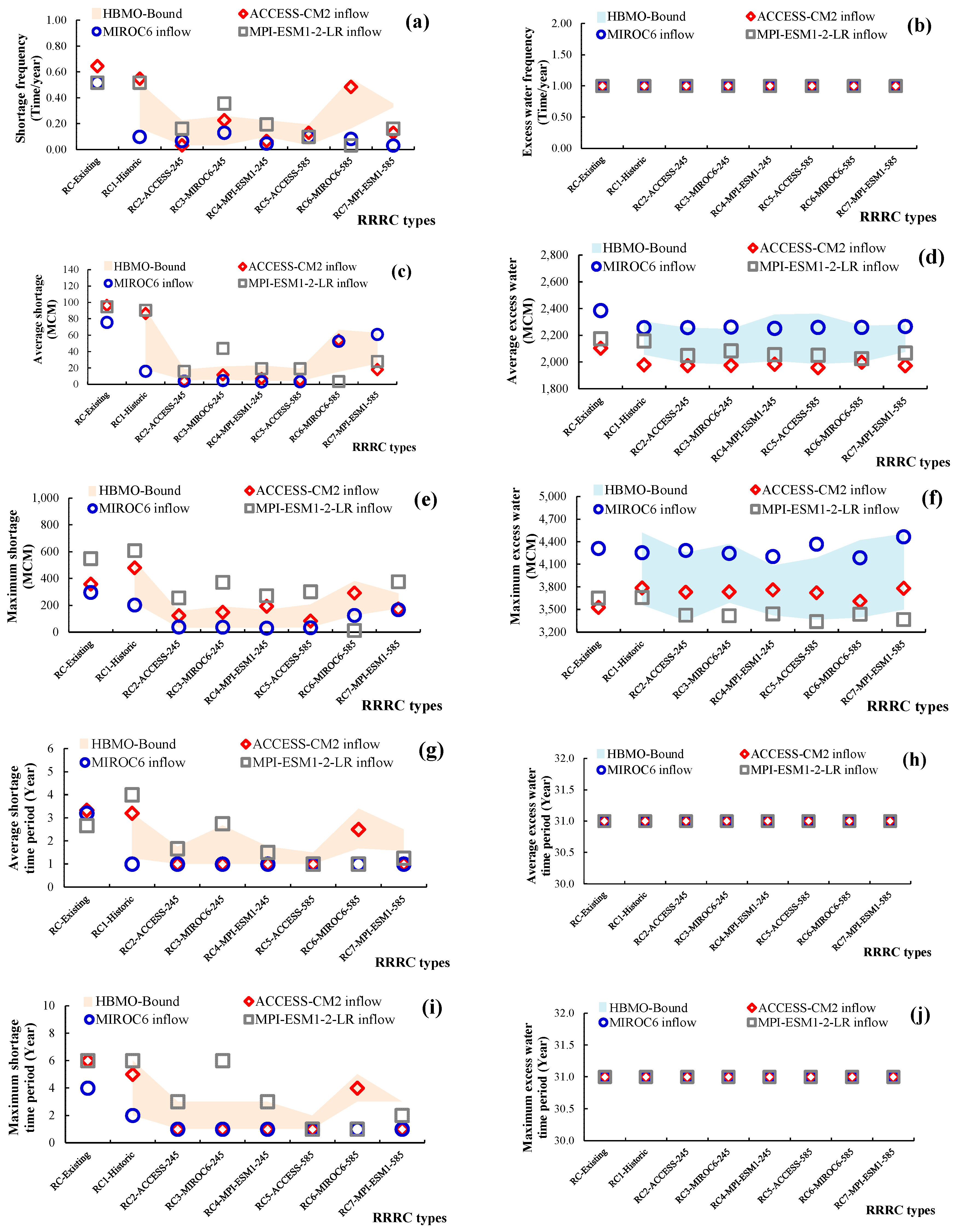
Efficiency assessment of RRRC developed by HO and HBMO is conducted with seven historical data sets on inflow (2000-2023), including RC1 developed from historical data and RC2-RC7 developed from future prediction data using three versions of GCMs (ACCESS-CM2, MIROC6, and MPI-ESM1-2-LR) under SSP245 and SSP585 to compare the efficiency with the existing rule curves currently applied to Ubonrat Reservoir operation. The assessment uses ten indicators, including five water shortage and five excess water to analyze for frequency, average magnitude, maximum magnitude, average duration, and maximum duration as presented in Figure 10, Figure 11 and Figure 12.
3.4.1. Efficiency of Rule Curves Developed by HO under Historic Inflow
The result of efficiency assessment of RRRC developed by HO and HBMO using historical inflow data (2000 - 2023) compared with the existing rule curve in terms of water shortage is presented in Figure 10 (a), (c), (e), (g), and (i). The frequency analysis of water shortage (Figure 10 (a)) indicates that all sets of RRRC can be lower in frequency than the existing at 0.786 times per year. RC5-HO shows the highest outstanding in efficiency that is decreasing from 242.554 MCM to122.286 MCM, or 50% decrease; HO is more efficient than HBMO in six out of seven cases. In case of highest water shortage (Figure 10 (e)), RC1-HO is the lowest at 810 MCM, 14% decreasing from the existing that has 942 MCM. In the event of time (Figure 10 (g) and (i)), RC5-HO shows outstanding improvement. The average shortage period decreases from 5.5 years to 2.182 years (60%) and maximum period decreases from 14 years to 3 years (79%).
The excess water assessment is shown in Figure 10 (b), (d), (f), (h), and (j). The result of frequency analysis for the excess water (Figure 10 (b)) indicates that RRRC gets slightly lower than the existing at 0.929 times per year; RC1-HO and RC4-HO are the lowest at 0.857 times per year (8% decrease). For the average excess water (Figure 10 (d)), HO is more efficient than HBMO in all cases, where RC1-HO is the lowest at 1,200.108 MCM or decreases 11% from the existing that has 1,346.281 MCM. In case of the maximum excess water (Figure 10 (f)), RC5-HO is the lowest that is 4,099.900 MCM. In time dimension (Figure 10 (h) and (j)), RC4-HO has significant improvement because the average excess water decreases from 10.4 years to 6.0 years (42%), and the maximum period decreases from 21 years to 11 years only (48%). The overall result of assessment affirms that RRRC developed by HO is more efficient than HBMO and the existing rule curve in decreasing both water shortage and excess water.
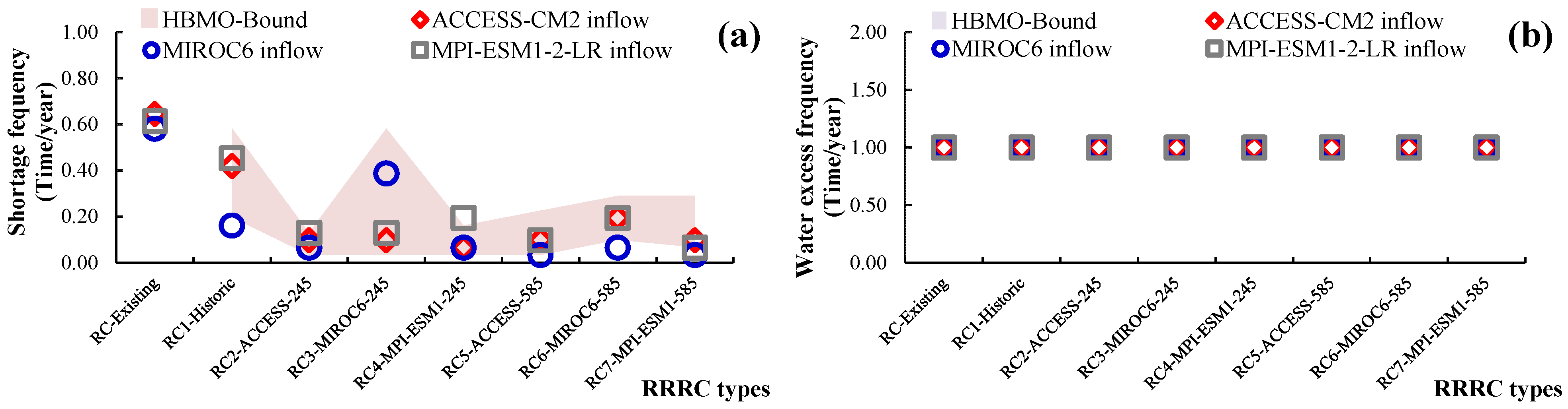
3.4.2. Efficiency of Rule Curves Developed by HO under Inflow of SSP245
In efficiency assessment of RRRC for the future inflow in three versions of GCMs (ACCESS-CM2, MIROC6, and MPI-ESM1-2-LR) under the route of greenhouse gas emission, SSP245 aims to analyze adaptability of the developed rule curves to future hydrological changes. This assessment uses predicted inflow data during 2024 – 2055 to simulate reservoir operation and compare the efficiency between RRRC developed by HO and the boundaries of HBMO and existing rule curve. The result of water shortage assessment is illustrated in Figure 11 (a), (c), (e), (g), and (i). The result of efficiency analysis reveals that RRRC developed by HO can significantly reduce more water shortage indicators than the existing rule curve. In terms of shortage frequency (Figure 11 (a)), RC2-ACCESS_245 is the highest efficient when testing with ACCESS-CM2 inflow. The frequency decreases from 0.645 to 0.032 times per year (95%) while RC4-MPI-ESM1_245 has the lowest frequency that is 0.045 times per year (91% decrease) when testing with MIROC6 inflow. In case of average water shortage (Figure 11 (c)), RC2-ACCESS_245 decreases from 96.387 MCM to 4.000 MCM (96%), and RC4-MPI-ESM1_245 is the minimum that is 3.155 MCM (96% decrease) when testing with MIROC6 inflow. For maximum water shortage (Figure 11 (e)), RC6-MIROC6_585 show a significant decrease when testing with MPI-ESM1-2-LR inflow, decreasing 98% from 549 MCM to 13 MCM, and RC5-ACCESS_585 shows the minimum of 83 MCM (or 77% decrease) when testing with ACCESS-CM2. In terms of time (Figure 11 (g) and (i)), RRRC can shorten both average and maximum time of water shortage to one year, which is possible minimum decreasing from the existing that has average period of 2.7-3.3 years and maximum of 4-6 years, or 70-83% decrease. The comparison of HBMO boundary (light orange area) indicates that HO is mostly within the boundary or below the lower boundary of HBMO, which represents equivalent or better reduction of water shortage.
According to the water excess assessment as shown in Figure 11 (b), (d), (f), (h), and (j), under the SSP245, the inflow is predicted to get higher continually, and the water excess happens annually during 31 years of simulation (2024-2055). As a result, the frequency is 1.0 time per year, and the fixed period is 31 years without difference among eight types of rule curves (Figure 11 (b), (h), and (j)). This reflects a physical limitation of the reservoir that cannot accommodate the higher inflow. In case of average water excess, however, all sets of HOs can reduce it 5-7% from the existing, where RC5-ACCESS_585 is the lowest or 1,958.344 MCM when testing with ACCESS-CM2 (7% decrease from 2,103.262 MCM) while RC6-MIROC6_585 becomes the lowest or 2,024.273 MCM when testing with MPI-ESM1-2-LR inflow (7% decrease). In the area of maximum water excess (Figure 11 (f)), RC5-ACCESS_585 is the lowest that is 3,340.313 MCM (9% decrease) when testing with MPI-ESM1-2-LR inflow while RC4-MPI-ESM1_245 is the lowest that is 4,205.717 MCM (2% decrease) when testing with MIROC6 inflow. In comparing with HBMO boundary (light blue area), HO is mostly in the boundary or below HBMO lower range. The assessment affirms that RRRC developed by HO is significantly efficient in reducing water shortage under climate change, and it partially reduces water excess even though the inflow becomes high throughout the prediction period.
Figure 11.
RRRC performance test results on future inflow from 3 GCMs under SSP245 comparing existing, HO and HBMO: (a) shortage frequency, (b) excess water frequency, (c) average shortage volume, (d) average excess volume, (e) maximum shortage volume, (f) maximum excess water volume, (g) maximum shortage time period, and (j) maximum excess water time period.
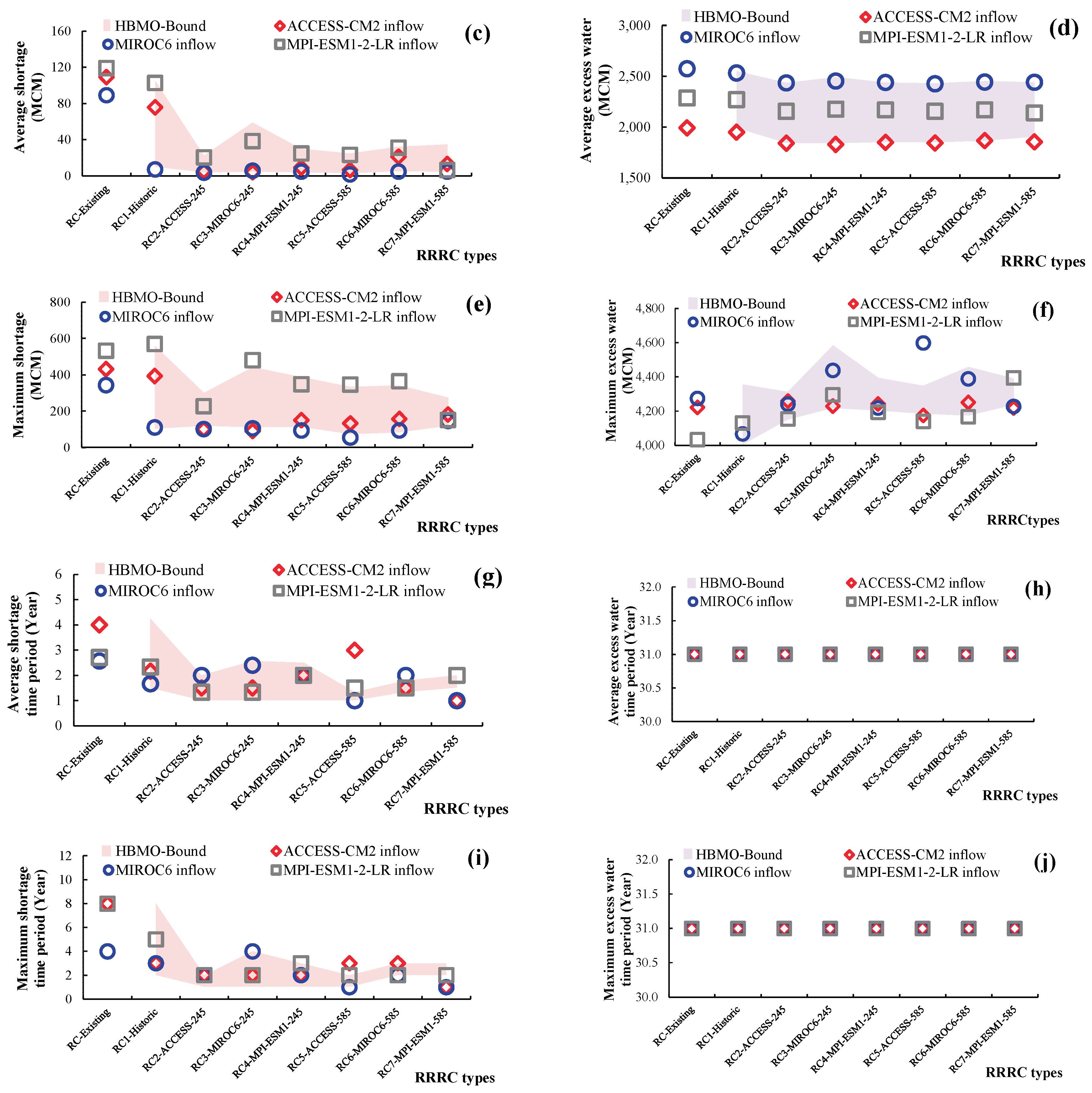
3.4.4. Efficiency of Rule Curves Developed by HO under Inflow of SSP585
The result of RRRC efficiency assessment under higher emission of greenhouse gas (SSP585) by simulating the Ubonrat Reservoir inflow during 2024 – 2055 in terms of water shortage is presented in Figure 12 (a), (c), (e), (g), and (i). It indicates that RRRC developed by HO still has the efficiency in reducing water shortage indicator significantly. For shortage frequency (Figure 12 (a)), RC5-ACCESS_585 and RC7-MPI-ESM1_585 give the best effectiveness when testing with MIROC6 inflow; the frequency is 0.032 times per year which decreases to 94% (or 0.581 times per year) from the existing rule curve. On the other hand, RC4-MPI-ESM1_245 shows minimum frequency of 0.065 times per year when comparing with ACCESS-CM2 inflow (or 90% decrease). In case of average water shortage (Figure 12 (c)), RC5-ACCESS_585 shows high potential result when testing with MIROC6 inflow. It decreases from 89.258 MCM to 1.742 MCM (or 98% decrease). Moreover, RC3-MIROC6_245 demonstrates high efficiency or 4.129 MCM (or 96% decrease) when testing with ACCESS-CM2. In maximum water shortage (Figure 12 (e)), RC5-ACCESS_585 is the lowest or 54 MCM (84% decrease) when testing with MIROC6 inflow while RC3-MIROC6_245 has 91 MCM (or 79% decrease) when testing with ACCESS-CM2 and RC7-MPI-ESM1_585 has 151 MCM (or 72% decrease) when testing with MPI-ESM1-2-LR inflow. In terms of shortage time (Figure 12 (g) and (i)), RC7-MPI-ESM1_585 is outstanding in its improvement. In other words, it reduces both average and maximum duration to only one year when testing with ACCESS-CM2 inflow and MIROC6 inflow respectively, and it decreases 75-88% comparing with the existing rule curve. Comparing the boundary of HBMO (light orange area) can affirm that most HOs are within the boundary or below lower boundary of HBMO.
The water excess assessment can be seen in Figure 12 (b), (d), (f), (h), and (j). The analysis result indicates that the water excess under SSP585 happens every year during 31 years of conducting simulation, so there is no difference between rule curves (Figure 12 (b), (h), and (j)). In terms of average water excess (Figure 12 (d)), all RRRCs developed by HO can reduce the volume to get lower the existing rule curve in all GCMs. RC3-MIROC6_245 is the lowest when testing with ACCESS-CM2 inflow, which is 1,828.633 MCM (decreases 8% or 1,992.348 MCM comparing with the existing rule curve). RC5-ACCESS_585 reaches the minimum or 2,424.903 MCM when testing with MIROC6 inflow (or decreases 6% or 2,573.126 MCM comparing with the existing) while RC7-MPI-ESM1_585 reaches the minimum or 2,137.399 MCM when testing with MPI-ESM1-2-LR inflow (or decreases 6% or 2,285.911 MCM comparing with the existing). Comparing with HBMO boundary (light blue area), most HOs are within the boundary or below the HBMO lower range, which indicate equivalent or better efficiency. In maximum water excess (Figure 12(f)), RC1-Historic is the highest efficient or 3,872.321 MCM when testing with ACCESS-CM2 (decreasing 8% from the existing or 4,221.712 MCM) and 4,066.477 MCM when testing with MIROC6 (decreasing 5% from the existing or 4,274.318 MCM). Nevertheless, all sets of HOs tested with MPI-ESM1-2-LR are 4,034.083 MCM higher than the existing. This demonstrates a challenge in managing the water excess under situations with high variation. Compared with HBMO boundary, most HOs are within the HBMO range. The overall result validates that RRRC developed by HO can maintain the efficiency to remarkedly reduce water shortage under higher emission of greenhouse gas, and it reduces average water excess comparable to SSP245.
Figure 12.
RRRC performance test results on future inflow under SSP585 comparing existing, HO and HBMO: (a) shortage frequency, (b) excess water frequency, (c) average shortage volume, (d) average excess volume, (e) maximum shortage volume, (f) maximum excess water volume, (g) maximum shortage time period, and (j) maximum excess water time period.
3.4.5. Efficiency Comparison of Resilience Reservoir Rule Curves under Climate Change
Efficiency comparison of RRRC developed by HO under three scenarios includes Historic Inflow, Future Inflow SSP245, and Future Inflow SSP585 as shown in Table 9. According to water shortage analysis, RRRC developed by HO can reduce indicator more significantly than the existing rule curve in all scenarios. When comparing with historic inflow, the maximum decrease of shortage frequency is 0.786 to 0.429 times/year (45% reduction), the decrease of average water shortage is 242.55 to 122.29 MCM (50% reduction), and the maximum shortage time period decreases from 14 to 3 years (79% reduction). Based on future inflow assessment under SSP245 and SSP585, the efficiency increases significantly, where the shortage frequency decreases to only 0.030-0.032 times per year (94-95% reduction), the average water shortage decreases to 1.74-3.16 MCM (96-98% reduction), and the maximum shortage time period decreases to 1 year (83-88% reduction). For this result, RRRC designed by using future inflow data is the most appropriate to handle climate change conditions. Moreover, HOs compared with HBMO boundary are within the or below HBMO Lower range in every scenario, especially in average shortage and duration. This can affirm that the efficiency of HO is higher than or equal to HBMO in terms of water shortage reduction.
In case of water excess, the comparison result shows a difference between scenarios. When comparing with historic inflow RRRC, water excess frequency decreases from 0.929 to 0.857 times per year (8% reduction), average water excess decreases from 1,346.28 to 1,200.11 MCM (11% reduction), and time period of maximum water excess decreases from 21 to 11 years (48% reduction). However, after testing with future inflow under SSP245 and SSP585, frequency and time period of the water excess cannot become lower due to consistently high volume of predicted future inflow throughout the simulation period. Nevertheless, RRRC can still decrease average water excess of 7-8% and maximum water excess of 8-9% when comparing with the existing rule curve, which is quantitatively significant for flood management. Compared with HBMO in terms of average excess, most HOs are below the HBMO lower range, which represent higher efficiency. The overall analysis result substantiates that RC5-ACCESS_585 and RC7-MPI-ESM1_585 show significant and constant in all scenarios, whereas RC1-Historic is highly efficient in case of comparing with historic Inflow especially in water excess reduction. Thus, decision on using RRRC should be dependent on predicted inflow in order to get high efficiency in reservoir management under uncertainty of climate change.
4. Conclusions
This study presents an integrated conceptual framework for Resilience Reservoir Rule Curves (RRRC) under uncertainty of climate change by integrating between GCMs from WEAP and Hippopotamus Optimization (HO), Ubonrat Reservoir operation policy, which is a major reservoir in the Upper Chi Watershed in Northeast of Thailand and always affected by draught and flood, was selected as a case study. The study uses three versions of GCMs, including ACCESS-CM2, MIROC6, and MPI-ESM1-2-LR, under SSP245 and SSP585 to simulate the reservoir inflow during 2024 – 2055. To simulate the inflow, WEAP, which was verified its accuracy by reservoir inflow and storage capacity simulations represented by acceptable indices including R2, NSE, RSR, and PBIAS, was used as a tool for future inflow simulation. Then the predicted inflow data were basically used for RRRC development employing HO technique inspired by hippopotamus’ risk avoidance behavior together with utilizing dual-objective function, which focuses on water shortage and water excess reduction.
The analysis results clearly present that RRRC developed by HO shows higher efficiency than HBMO and the existing rule curve in every scenario. In comparing with historical inflow (2000 – 2023), HO can reduce average water shortage and water excess more than the existing rule curve under future climate change. As a result, HO has a significant advantage. In SSP245, the rule curves developed by HO can reduce water shortage frequency and maximum water shortage below the existing rule curve. On the other hand, in SSP585, the average water shortage becomes lower than SSP245 although its water shortage frequency slightly increases. This result reflects that HO is well-adapted to precipitation variable, which is higher under high level of greenhouse gas emission. In addition, a water excess in SSP585 is lower than in SSP245, which indicates potential of HO to establish a balance between water shortage and water excess management. In comparing ten indicators of efficiency between HO and HBMO (five for water shortage and five for water excess), HO is lower or at the lower bound of the resulting range from HBMO in almost all scenarios. This reflects stability and consistency of HO to seek optimal solution.
The findings of this study can be concluded into four main issues. (1) GCMs-WEAP-HO integration framework can develop resilient and adaptable RRRC under uncertainty of climate change especially in risk reduction of water shortage in the dry season and flood mitigation in the rainy season. (2) HO can demonstrate its efficiency that is greater than HBMO and existing rule curve in every scenario particularly in reduction of water excess under historical inflow and reduction of average water shortage under SSP245 and SSP585. (3) Comparative analysis between SSP245 and SSP585 has revealed some crucial points. SSP245 has an advantage in preventing severe water shortage while SSP585 is higher efficient in reducing average water shortage and regulating excess water. (4) RRRCs developed by HO represents an optimal balance for water resource management under different climate changes. The developed framework can be applied to other reservoirs experiencing similar problem and scaled up to considering other factors, such as land use change, future demand of water use, and various policies on water management for sustainable resilience enhancement of water resource system against impacts of climate change.
Author Contributions
Conceptualization, H.P. and R.H.; methodology, H.P.; software, H.P., R.T., R.N. and S.W; validation, H.P. and R.T.; formal analysis, H.P., R.H. and R.N.; investigation, J.S. and K.S.; resources, K.S.; data curation, H.P and R.H.; writing—original draft preparation, H.P. and R.H; writing—review and editing, A.K and S.K; visualization, S.W.; supervision, A.K. and S.K.; project administration, R.H., A.K., S.K., K.S. and J.S.; funding acquisition, R.H.
Funding
This research project was financially supported by Thailand Science Research and Innovation (TSRI).
Data Availability Statement
The original contributions presented in this study are included in the article. Further inquiries can be directed to the corresponding authors.
Acknowledgments
The researchers would like to thank the Faculty of Engineering, Mahasarakham University (MSU) and Rajamangala University of Technology Isan (RMUTI), Khon Kaen Campus for enabling the successful completion of this research. Special thanks are also due to the Electricity Generating Authority of Thailand (EGAT) for providing hydrological data and operational records of the Ubolrat Reservoir, the Thai Meteorological Department (TMD) for meteorological data, the Land Development Department (LDD) for land use and soil data, all of which were crucial to this research.
Conflicts of Interest
The authors declare no conflicts of interest.
Abbreviations
The following abbreviations are used in this manuscript:
| SDG | Sustainable Development Goals |
| WEAP | Water Evaluation and Planning |
| GCMs | General Circulation Models |
| SSP | Shared Socioeconomic Pathways |
| CMIP6 | Coupled Model Intercomparison Project Phase 6 |
| NEX-GDDP | NASA Earth Exchange Global Daily Downscaled Projections |
| ACCESS-CM2 | Australian Community Climate and Earth System Simulator, Coupled Model version 2 |
| MIROC6 | Model for Interdisciplinary Research on Climate, version 6 |
| MPI-ESM1-2-LR | Max Planck Institute Earth System Model (Version 1.2) - Low Resolution |
| HO | Hippopotamus Optimization |
| HBMO | Honey Bee Mating Optimization |
| RRRC | Resilience Reservoir Rule Curve |
| RC | Rule Curves |
| SRTM | Shuttle Radar Topography Mission |
| EGAT | Electricity Generating Authority of Thailand |
| RID | Royal Irrigation Department |
| LDD | Land Development Department |
| TMD | Thai Meteorology Department |
| MCM | Million Cubic Meters |
| sq.km | Square Kilometers |
References
- Water for Development and Development for Water: Realizing the Sustainable Development Goals (SDGs) Vision. Aquat. Procedia 2016, 6, 106–110. [CrossRef]
- Evaristo, J.; Jameel, Y.; Tortajada, C.; Wang, R.Y.; Horne, J.; Neukrug, H.; David, C.P.; Fasnacht, A.M.; Ziegler, A.D.; Biswas, A. Water Woes: the Institutional Challenges in Achieving SDG 6. Sustain. Earth. Rev. 2023, 6(1), 13. [Google Scholar] [CrossRef]
- Songsaengrit, S.; Kangrang, A. Dynamic Rule Curves and Streamflow under Climate Change for Multipurpose Reservoir Operation using Honey-bee Mating Optimization. Sustainability 2022, 14(14), 8599. [Google Scholar] [CrossRef]
- Kangrang, A.; Prasanchum, H.; Sriworamas, K.; Ashrafi, S.M.; Hormwichian, R.; Techarungruengsakul, R.; Ngamsert, R. Application of Optimization Techniques for Searching Optimal Reservoir Rule Curves: A Review. Water 2023, 15(9), 1669. [Google Scholar] [CrossRef]
- Beça, P.; Rodrigues, A.C.; Nunes, J.P.; Diogo, P; Mujtaba, B. Optimizing Reservoir Water Management in a Changing Climate. Water Resour. Manag. 2023, 37(9), 3423–3437. [Google Scholar] [CrossRef]
- Yao, A.B.; Mangoua, O.M.J.; Georges, E.S.; Kane, A.; Goula, B.T.A. Using “Water Evaluation and Planning” (WEAP) Model to Simulate Water Demand in Lobo Watershed (Central-Western Cote d'Ivoire). J. Water Resour. Prot. 2021, 13, 216–235. [Google Scholar] [CrossRef]
- Abera Abdi, D.; Ayenew, T. Evaluation of the WEAP Model in Simulating Subbasin Hydrology in the Central Rift Valley Basin, Ethiopia. Ecol. Process. 2021, 10, 41. [Google Scholar] [CrossRef]
- Ougahi, J.H.; Karim, S.; Mahmood, S.A. Application of the SWAT Model to Assess Climate and Land Use/cover Change Impacts on Water Balance Components of the Kabul River Basin, Afghanistan. J. Water Clim. Chang. 2022, 13, 3977–3999. [Google Scholar] [CrossRef]
- Aloui, S.; Mazzoni, A.; Elomri, A.; Aouissi, J.; Boufekane, A.; Zghibi, A. A Review of Soil and Water Assessment Tool (SWAT) Studies of Mediterranean Catchments: Applications, Feasibility, and Future Directions. J. Environ. Manage. 2023, 326, 116799. [Google Scholar] [CrossRef]
- Pareta, K. Hydrological Modelling of Largest Braided River of India Using MIKE Hydro River Software with Rainfall Runoff, Hydrodynamic and Snowmelt Modules. J. Water Clim. Chang. 2023, 14(4), 1314–1338. [Google Scholar] [CrossRef]
- Zhang, J.; Zhang, M.; Song, Y.; Lai, Y. Hydrological Simulation of the Jialing River Basin using the MIKE SHE Model in changing climate. J. Water Clim. Chang. 2021, 12, 2495–2514. [Google Scholar] [CrossRef]
- Berhe, F.T.; Melesse, A.M.; Hailu, D.; Sileshi, Y. MODSIM-based Water Allocation Modeling of Awash River Basin, Ethiopia. CATENA 2013, 109, 118–128. [Google Scholar] [CrossRef]
- Supharatid, S.; Nafung, J. Projected Drought Conditions by CMIP6 Multimodel Ensemble over Southeast Asia. J. Water Clim. Chang. 2021, 12(7), 3330–3354. [Google Scholar] [CrossRef]
- Zhao, T.; Dai, A. CMIP6 Model-projected Hydroclimatic and Drought Changes and Their Causes in the Twenty-First Century. J. Clim. 2022, 35, 897–921. [Google Scholar]
- Lai, V.; Huang, Y.F.; Koo, C.H.; Ahmed, A.N.; El-Shafie, A. A Review of Reservoir Operation Optimisations: from Traditional Models to Metaheuristic Algorithms. Arch. Comput. Methods Eng. 2022, 29(5), 3435–3457. [Google Scholar] [CrossRef] [PubMed]
- Prasanchum, H.; Kangrang, A. Optimal Reservoir Rule Curves under Climatic and Land Use Changes for Lampao Dam Using Genetic Algorithm. KSCE J. Civ. Eng. 2018, 22(1), 351–364. [Google Scholar] [CrossRef]
- Ahmadianfar, I.; Zamani, R. Assessment of the Hedging Policy on Reservoir Operation for Future Drought Conditions under Climate Change. Clim. Chang. 2020, 159(2), 253–268. [Google Scholar] [CrossRef]
- Ashofteh, P.S.; Bozorg-Haddad, O.; Loáiciga, H.A. Logical Genetic Programming (LGP) Application to Water Resources Management. Environ. Monit. Assess. 2019, 192(1), 34. [Google Scholar] [CrossRef]
- Afshar, A.; Massoumi, F.; Afshar, A.; Mariño, M.A. State of the Art Review of Ant Colony Optimization Applications in Water Resource Management. Water Resour. Manag. 2015, 29, 3891–3904. [Google Scholar] [CrossRef]
- Garousi-Nejad, I.; Bozorg-Haddad, O.; Loáiciga, H.A.; Mariño, M.A. Application of the Firefly Algorithm to Optimal Operation of Reservoirs with the Purpose of Irrigation Supply and Hydropower Production. J. Irrig. Drain. Eng. 2016, 142(10), 04016041. [Google Scholar] [CrossRef]
- Ehteram, M.; Mousavi, S.F.; Karami, H.; Farzin, S.; Celeste, A.B.; Shafie, A.E. Bat Algorithm for Dam–Reservoir Operation. Environ. Earth Sci. 2018, 77(13), 510. [Google Scholar] [CrossRef]
- Donyaii, A; Sarraf, A.; Ahmadi, H. Water Reservoir Multiobjective Optimal Operation Using Grey Wolf Optimizer. Shock Vib. 2020, 8870464. [Google Scholar] [CrossRef]
- Jahandideh-Tehrani, M.; Bozorg-Haddad, O.; Loáiciga, H.A. Application of Particle Swarm Optimization to Water Management: an Introduction and Overview. Environ. Monit. Assess. 2020, 192(5), 281. [Google Scholar] [CrossRef] [PubMed]
- Meng, X.; Chang, J.; Wang, X.; Wang, Y. Multi-Objective Hydropower Station Operation Using an Improved Cuckoo Search Algorithm. Energy 2019, 168, 425–439. [Google Scholar] [CrossRef]
- Bashiri-Atrabi, H.; Qaderi, K.; Rheinheimer, D.E.; Sharifi, E. Application of Harmony Search Algorithm to Reservoir Operation Optimization. Water Resour. Manag. 2015, 29(15), 5729–5748. [Google Scholar] [CrossRef]
- Emami, M.; Nazif, S.; Mousavi, S.F.; Karami, H.; Daccache, A. A Hybrid Constrained Coral Reefs Optimization Algorithm with Machine Learning for Optimizing Multi-Reservoir Systems Operation. J. Environ. Manag. 2021, 286, 112250. [Google Scholar] [CrossRef]
- Asadieh, B.; Afshar, A. Optimization of Water-Supply and Hydropower Reservoir Operation Using the Charged System Search Algorithm. Hydrology 2019, 6(1), 5. [Google Scholar] [CrossRef]
- Giuliani, M.; Lamontagne, J.R.; Reed, P.M.; Castelletti, A. A State-of-the-Art Review of Optimal Reservoir Control for Managing Conflicting Demands in a Changing World. Water Resour. Res. 2021, 57(12), e2021WR029927. [Google Scholar] [CrossRef]
- Hormwichian, R.; Kaewplang, S.; Kangrang, A.; Supakosol, J.; Boonrawd, K.; Sriworamat, K.; Muangthong, S.; Songsaengrit, S.; Prasanchum, H. Understanding the Interactions of Climate and Land Use Changes with Runoff Components in Spatial-Temporal Dimensions in the Upper Chi Basin, Thailand. Water 2023, 15(19), 3345. [Google Scholar] [CrossRef]
- Chadwick, C.; Gironas, J.; Barría, P.; Vicuña, S.; Meza, F. Assessing Reservoir Performance under Climate Change. When Is It Going to Be Too Late If Current Water Management Is Not Changed? Water 2020, 13(1), 64. [Google Scholar] [CrossRef]
- Touseef, M.; Chen, L.; Yang, W. Assessment of Surface Water Availability under Climate Change Using Coupled SWAT-WEAP in Hongshui River Basin, China. ISPRS Int. J. Geo-Inf. 2021, 10(5), 298. [Google Scholar] [CrossRef]
- Hadri, A.; Saidi, M.E.M.; El Khalki, E.M.; Aachrine, B.; Saouabe, T.; Elmaki, A.A. Integrated Water Management under Climate Change through the Application of the WEAP Model in a Mediterranean Arid Region. J. Water Clim. Chang. 2022, 13(6), 2414–2442. [Google Scholar] [CrossRef]
- Hatamkhani, A.; Shourian, M.; Moridi, A. Optimal Design and Operation of a Hydropower Reservoir Plant Using a WEAP-Based Simulation–Optimization Approach. Water Resour. Manag. 2021, 35(5), 1637–1652. [Google Scholar] [CrossRef]
- Allani, M.; Mezzi, R.; Zouabi, A.; Béji, R.; Joumade-Mansouri, F.; Hamza, M.E.; Sahli, A. Impact of Future Climate Change on Water Supply and Irrigation Demand in a Small Mediterranean Catchment. Case Study: Nebhana Dam System, Tunisia. J. Water Clim. Chang. 2020, 11(4), 1724–1747. [Google Scholar] [CrossRef]
- Chakraei, I.; Safavi, H.R.; Dandy, G.C.; Golmohammadi, M.H. Integrated Simulation-Optimization Framework for Water Allocation Based on Sustainability of Surface Water and Groundwater Resources. J. Water Resour. Plan. Manag. 2021, 147(3), 05021001. [Google Scholar] [CrossRef]
- Ahmed, N.; Lü, H.; Ahmed, S.; Nabi, G.; Wajid, M.A.; Shakoor, A.; Farid, H.U. Irrigation Supply and Demand, Land Use/Cover Change and Future Projections of Climate, in Indus Basin Irrigation System, Pakistan. Sustainability 2021, 13(16), 8695. [Google Scholar] [CrossRef]
- Opere, A.O.; Waswa, R.; Mutua, F.M. Assessing the Impacts of Climate Change on Surface Water Resources Using WEAP Model in Narok County, Kenya. Front. Water 2022, 3, 789340. [Google Scholar] [CrossRef]
- Agarwal, S.; Patil, J.P.; Goyal, V.C.; Singh, A. Assessment of Water Supply–Demand Using Water Evaluation and Planning (WEAP) Model for Ur River Watershed, Madhya Pradesh, India. J. Inst. Eng. (India) Ser. A 2019, 100(1), 21–32. [Google Scholar] [CrossRef]
- Abungba, J.A.; Adjei, K.A.; Gyamfi, C.; Odai, S.N.; Pingale, S.M.; Khare, D. Implications of Land Use/Land Cover Changes and Climate Change on Black Volta Basin Future Water Resources in Ghana. Sustainability 2022, 14(19), 12383. [Google Scholar] [CrossRef]
- Tayyebi, M.; Sharafati, A.; Nazif, S.; Raziei, T. Assessment of Adaptation Scenarios for Agriculture Water Allocation under Climate Change Impact. Stoch. Environ. Res. Risk Assess. 2023, 37(9), 3527–3549. [Google Scholar] [CrossRef]
- Mesgari, E.; Hosseini, S.A.; Hemmesy, M.S.; Houshyar, M.; Partoo, L.G. Assessment of CMIP6 Models' Performances and Projection of Precipitation Based on SSP Scenarios over the MENAP Region. J. Water Clim. Chang. 2022, 13(10), 3607–3619. [Google Scholar] [CrossRef]
- Lei, Y.; Chen, J.; Xiong, L. A Comparison of CMIP5 and CMIP6 Climate Model Projections for Hydrological Impacts in China. Hydrol. Res. 2023, 54(3), 330–347. [Google Scholar] [CrossRef]
- Moghadam, S.H.; Ashofteh, P.S.; Loáiciga, H.A. Optimal Water Allocation of Surface and Ground Water Resources under Climate Change with WEAP and IWOA Modeling. Water Resour. Manag. 2022, 36(9), 3181–3205. [Google Scholar] [CrossRef]
- Abbas, S.A.; Xuan, Y.; Bailey, R.T. Assessing Climate Change Impact on Water Resources in Water Demand Scenarios Using SWAT-MODFLOW-WEAP. Hydrology 2022, 9(10), 164. [Google Scholar] [CrossRef]
- Try, S.; Tanaka, S.; Tanaka, K.; Sayama, T.; Khujanazarov, T.; Oeurng, C. Comparison of CMIP5 and CMIP6 GCM Performance for Flood Projections in the Mekong River Basin. J. Hydrol. Reg. Stud. 2022, 40, 101035. [Google Scholar] [CrossRef]
- Ly, S.; Sayama, T.; Try, S. Integrated Impact Assessment of Climate Change and Hydropower Operation on Streamflow and Inundation in the Lower Mekong Basin. Prog. Earth Planet. Sci. 2023, 10(1), 55. [Google Scholar] [CrossRef]
- Sheikha-BagemGhaleh, S.; Babazadeh, H.; Rezaie, H.; Sarai-Tabrizi, M. The Effect of Climate Change on Surface and Groundwater Resources Using WEAP-MODFLOW Models. Appl. Water Sci. 2023, 13(6), 121. [Google Scholar] [CrossRef]
- Ismail Dhaqane, A.; Murshed, M.F.; Mourad, K.A.; Abd Manan, T.S.B. Assessment of the Streamflow and Evapotranspiration at Wabiga Juba Basin Using a Water Evaluation and Planning (WEAP) Model. Water 2023, 15(14), 2594. [Google Scholar] [CrossRef]
- RaziSadath, P.V.; RinishaKartheeshwari, M.; Elango, L. WEAP Model Based Evaluation of Future Scenarios and Strategies for Sustainable Water Management in the Chennai Basin, India. AQUA—Water Infrastruct. Ecosyst. Soc. 2023, 72(11), 2062–2080. [Google Scholar] [CrossRef]
- Amiri, M.H.; Mehrabi Hashjin, N.; Montazeri, M.; Mirjalili, S.; Khodadadi, N. Hippopotamus Optimization Algorithm: A Novel Nature-Inspired Optimization Algorithm. Sci. Rep. 2024, 14(1), 5032. [Google Scholar] [CrossRef]
- Han, T.; Wang, H.; Li, T.; Liu, Q.; Huang, Y. MHO: A Modified Hippopotamus Optimization Algorithm for Global Optimization and Engineering Design Problems. Biomimetics 2025, 10(2), 90. [Google Scholar] [CrossRef]
- Aribowo, W.; Mzili, T.; Sabo, A. Enhanced Hippopotamus Optimization Algorithm for Power System Stabilizers. Indones. J. Electr. Eng. Comput. Sci. 2025, 38(1), 22–31. [Google Scholar] [CrossRef]
- Maurya, P.; Tiwari, P.; Pratap, A. Application of the Hippopotamus Optimization Algorithm for Distribution Network Reconfiguration with Distributed Generation Considering Different Load Models for Enhancement of Power System Performance. Electr. Eng. 2025, 107(4), 3909–3946. [Google Scholar] [CrossRef]
- Kumar, V.; Yadav, S.M. A State-of-the-Art Review of Heuristic and Metaheuristic Optimization Techniques for the Management of Water Resources. Water Supply 2022, 22(4), 3702–3728. [Google Scholar] [CrossRef]
- Tsakiris, G.P.; Loucks, D.P. Adaptive Water Resources Management Under Climate Change: An Introduction. Water Resour. Manag. 2023, 37(6), 2221–2233. [Google Scholar] [CrossRef]
- Tanguy, M.; Eastman, M.; Magee, E.; Barker, L.J.; Chitson, T.; Ekkawatpanit, C.; Goodwin, D.; Hannaford, J.; Holman, I.; Pardthaisong, L.; Parry, S.; Rey Vicario, D.; Visessri, S. Indicator-to-Impact Links to Help Improve Agricultural Drought Preparedness in Thailand. Nat. Hazards Earth Syst. Sci. 2023, 23, 2419–2441. [Google Scholar] [CrossRef]
- Thrasher, B.; Wang, W.; Michaelis, A.; Melton, F.; Lee, T.; Nemani, R. NASA Global Daily Downscaled Projections, CMIP6. Sci. Data 2022, 9(1), 262. [Google Scholar] [CrossRef] [PubMed]
- O'Neill, B.C.; Tebaldi, C.; van Vuuren, D.P.; Eyring, V.; Friedlingstein, P.; Hurtt, G.; Knutti, R.; Kriegler, E.; Lamarque, J.-F.; Lowe, J.; Meehl, G.A.; Moss, R.; Riahi, K.; Sanderson, B.M. The Scenario Model Intercomparison Project (ScenarioMIP) for CMIP6. Geosci. Model Dev. 2016, 9, 3461–3482. [Google Scholar] [CrossRef]
- Wu, F.; Jiao, D.; Yang, X.; Cui, Z.; Zhang, H.; Wang, Y. Evaluation of NEX-GDDP-CMIP6 in Simulation Performance and Drought Capture Utility over China – Based on DISO. Hydrol. Res. 2023, 54(5), 703–721. [Google Scholar] [CrossRef]
- Dix, M.; Bi, D.; Dobrohotoff, P.; Fiedler, R.; Harman, I.; Law, R.; Mackallah, C.; Marsland, S.; O'Farrell, S.; Rashid, H.; Srbinovsky, J. CSIRO-ARCCSS ACCESS-CM2 model output prepared for CMIP6 ScenarioMIP. 2019. [Google Scholar]
- Shiogama, H.; Abe, M.; Tatebe, H. MIROC MIROC6 model output prepared for CMIP6 ScenarioMIP ssp245. 2019, (No Title).
- Wieners, K.H.; Giorgetta, M.; Jungclaus, J.; Reick, C.; Esch, M.; Bittner, M.; Gayler, V.; Haak, H.; de Vrese, P.; Raddatz, T.; Mauritsen, T. MPI-m MPIESM1. 2-LR model output prepared for CMIP6 ScenarioMIP. 2019, (No Title).
- Shaabani, M.K.; Abedi-Koupai, J.; Eslamian, S.S.; Gohari, S.A.R. Simulation of the Effects of Climate Change, Crop Pattern Change, and Developing Irrigation Systems on the Groundwater Resources by SWAT, WEAP and MODFLOW Models: A Case Study of Fars Province, Iran. Environ. Dev. Sustain. 2024, 26(4), 10485–10511. [Google Scholar] [CrossRef]
- Tena, T.M.; Mwaanga, P.; Nguvulu, A. Hydrological Modelling and Water Resources Assessment of Chongwe River Catchment using WEAP model. Water 2019, 11(4), 839. [Google Scholar] [CrossRef]
- Hormwichian, R.; Tongsiri, J.; Kangrang, A. Multipurpose Rule Curves for Multipurpose Reservoir by Conditional Genetic algorithm. Int. Rev. Civ. Eng. 2018, 9(3), 114. [Google Scholar] [CrossRef]
- Sriworamas, K.; Prasanchum, H.; Ashrafi, S.M.; Hormwichian, R.; Techarungruengsakul, R.; Ngamsert, R.; Chaiyason, T.; Kangrang, A. Concern Condition for Applying Optimization Techniques with Reservoir Simulation Model for Searching Optimal Rule Curves. Water 2023, 15(13), 2501. [Google Scholar] [CrossRef]
- Eryani, I.G.A.P. Sensitivity Analysis in Parameter Calibration of the WEAP Model for Integrated Water Resources Management in Unda Watershed. Civ. Eng. Archit. 2022, 455–469. [Google Scholar] [CrossRef]
- Moriasi, D.N.; Gitau, M.W.; Pai, N.; Daggupati, P. Hydrologic and Water Quality Models: Performance Measures and Evaluation Criteria. Trans. ASABE 2015, 58(6), 1763–1785. [Google Scholar]
- Fernández-Alberti, S.; Abarca-del-Río, R.; Bornhardt, C.; Ávila, A. Development and Validation of a Model to Evaluate the Water Resources of a Natural Protected Area as a Provider of Ecosystem Services in a Mountain Basin in Southern Chile. Front. Earth Sci. 2021, 8, 539905. [Google Scholar] [CrossRef]
- Sahu, A.; Verma, M.K.; Kumre, S.K. A Hybrid Technique to Enhance the Rainfall-Runoff Prediction of Physical and Data-Driven Model: A Case Study of Upper Narmada River Sub-basin, India. Sci. Rep. 2024, 14, 26368. [Google Scholar]
- Dash, S.S.; Sahoo, B.; Raghuwanshi, N.S. An Integrated Reservoir Operation Framework for Enhanced Water Resources Planning. Sci. Rep. 2023, 13, 21720. [Google Scholar] [CrossRef] [PubMed]
Figure 1.
Study area.
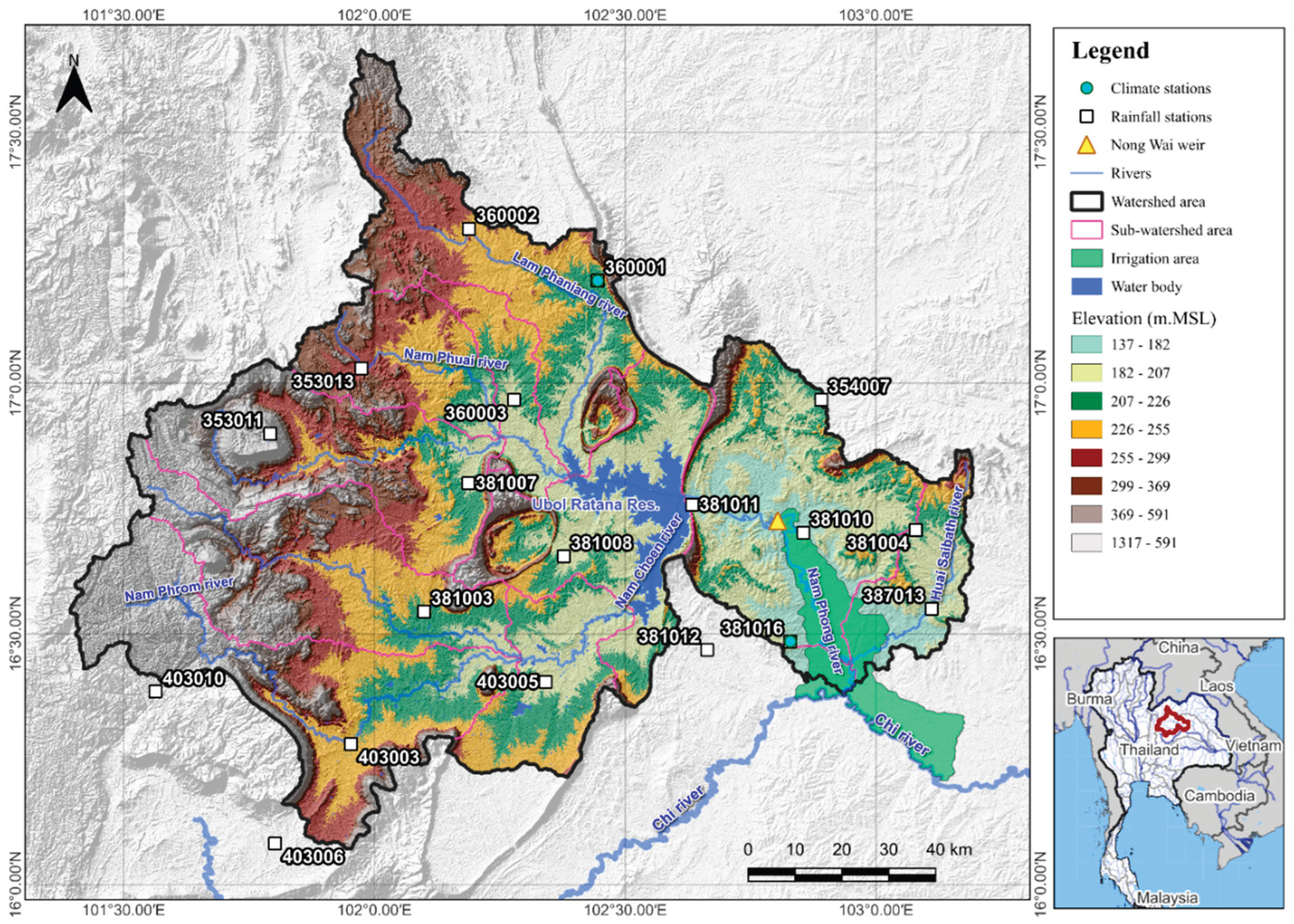
Figure 2.
Spatial data of watershed inputted into WEAP.
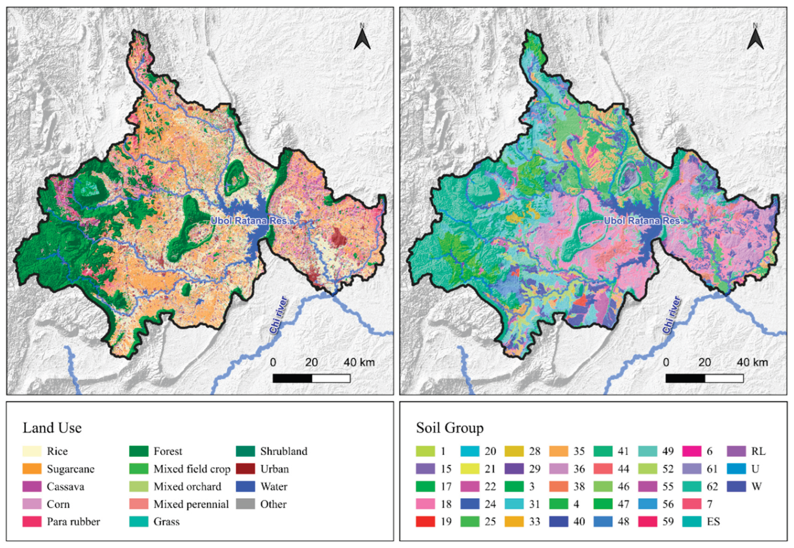
Figure 3.
Flowchart of HO connected with reservoir simulation model.
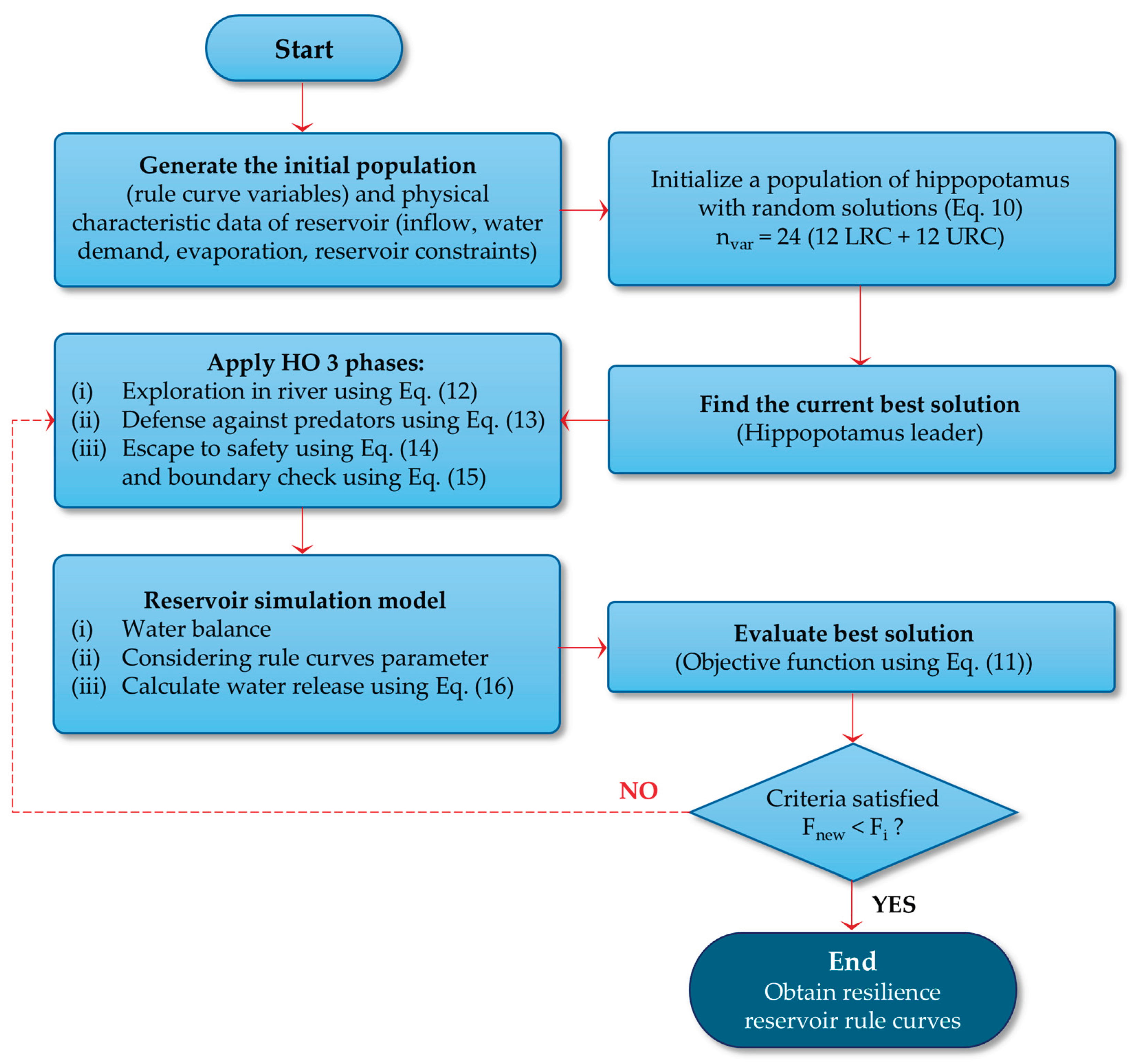
Figure 4.
Monthly average precipitation and temperature in each period, (a) monthly average precipitation in SSP245, (b) monthly average precipitation in SSP585, (c) monthly average temperature in SSP245, and (d) monthly average temperature in SSP585.
Figure 4.
Monthly average precipitation and temperature in each period, (a) monthly average precipitation in SSP245, (b) monthly average precipitation in SSP585, (c) monthly average temperature in SSP245, and (d) monthly average temperature in SSP585.
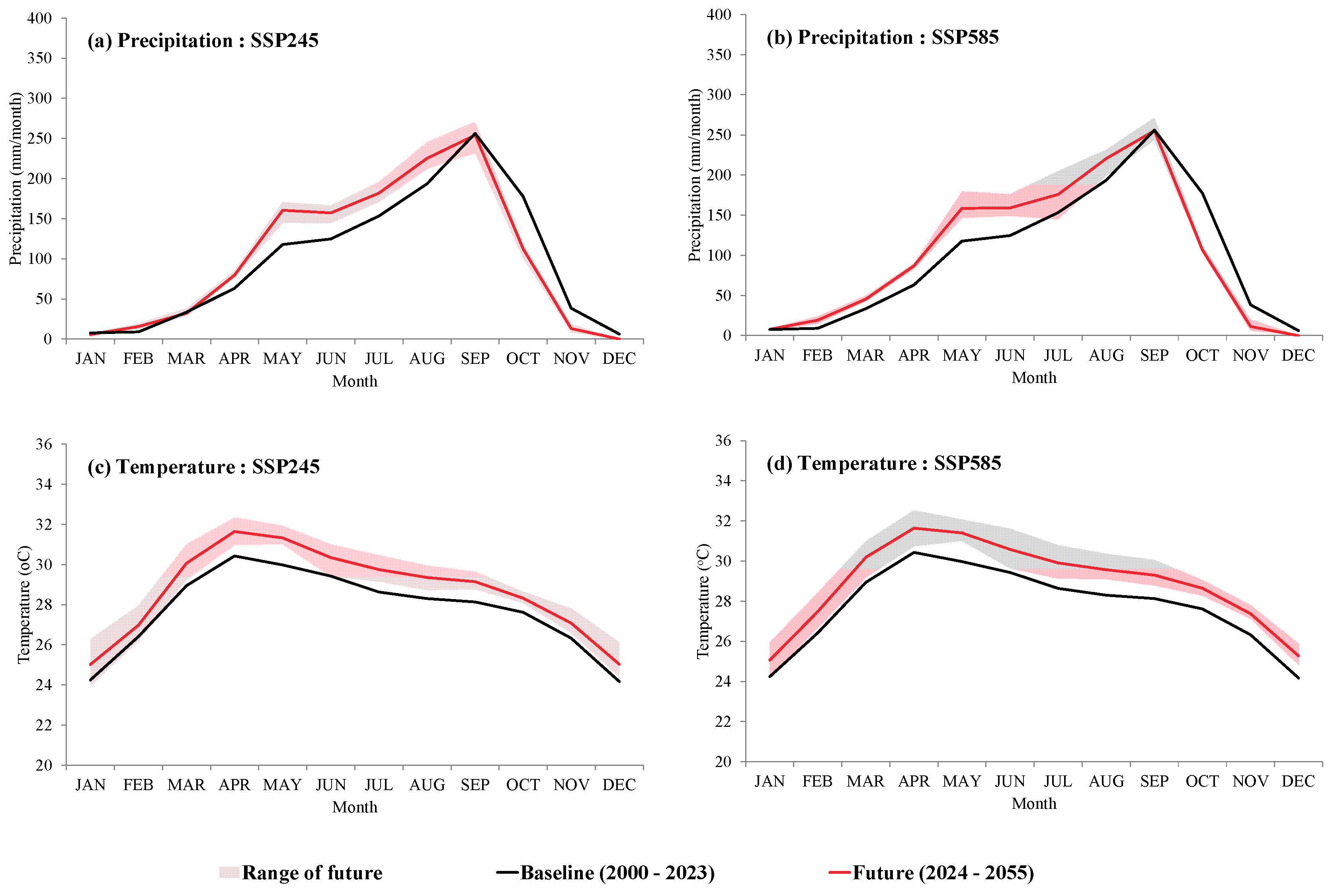
Figure 5.
Results of WEAP calibration and validation: (a) reservoir inflow, and (b) storage volume.
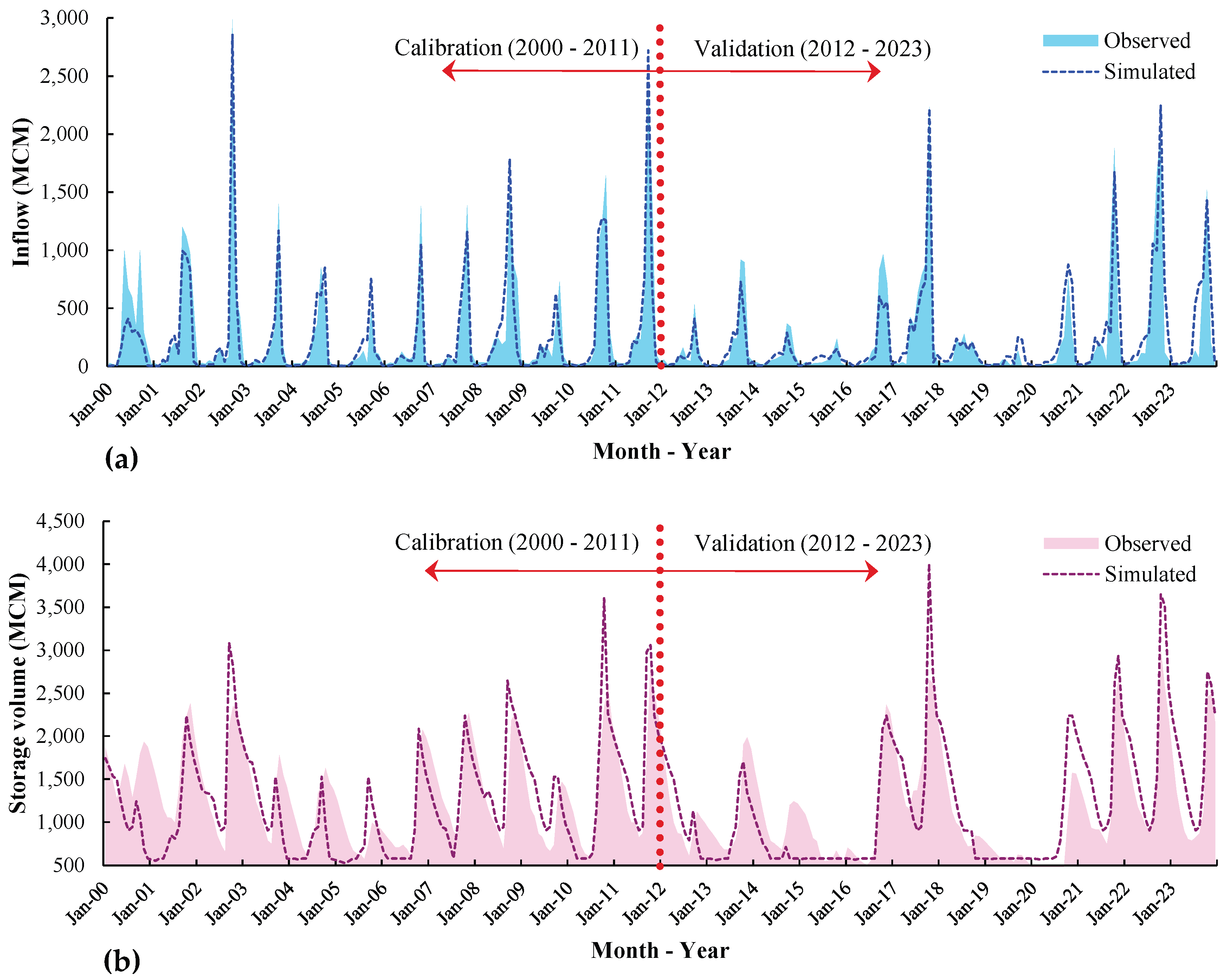
Figure 10.
RRRC performance test results under historic inflow comparing existing, HBMO and HO: (a) shortage frequency, (b) excess water frequency, (c) average shortage volume, (d) average excess volume, (e) maximum shortage volume, (f) maximum excess water volume, (g) maximum shortage time period, and (j) maximum excess water time period.
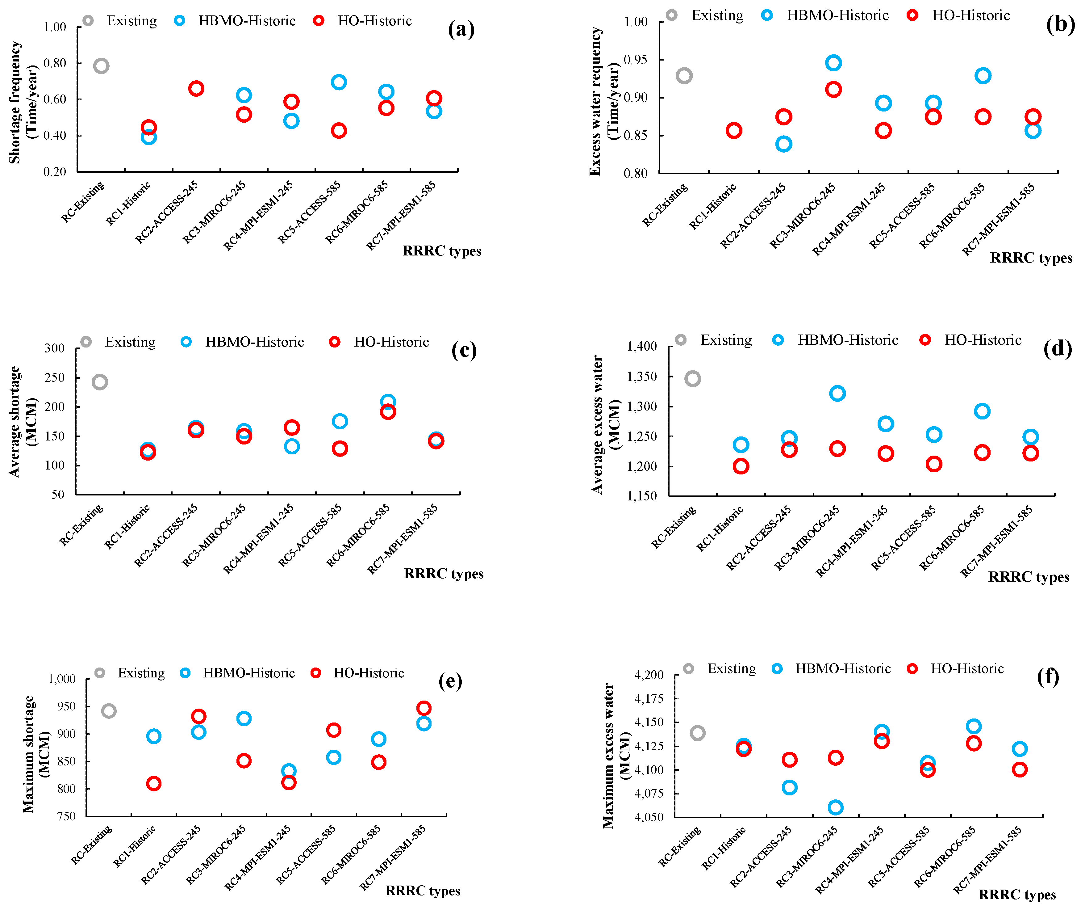
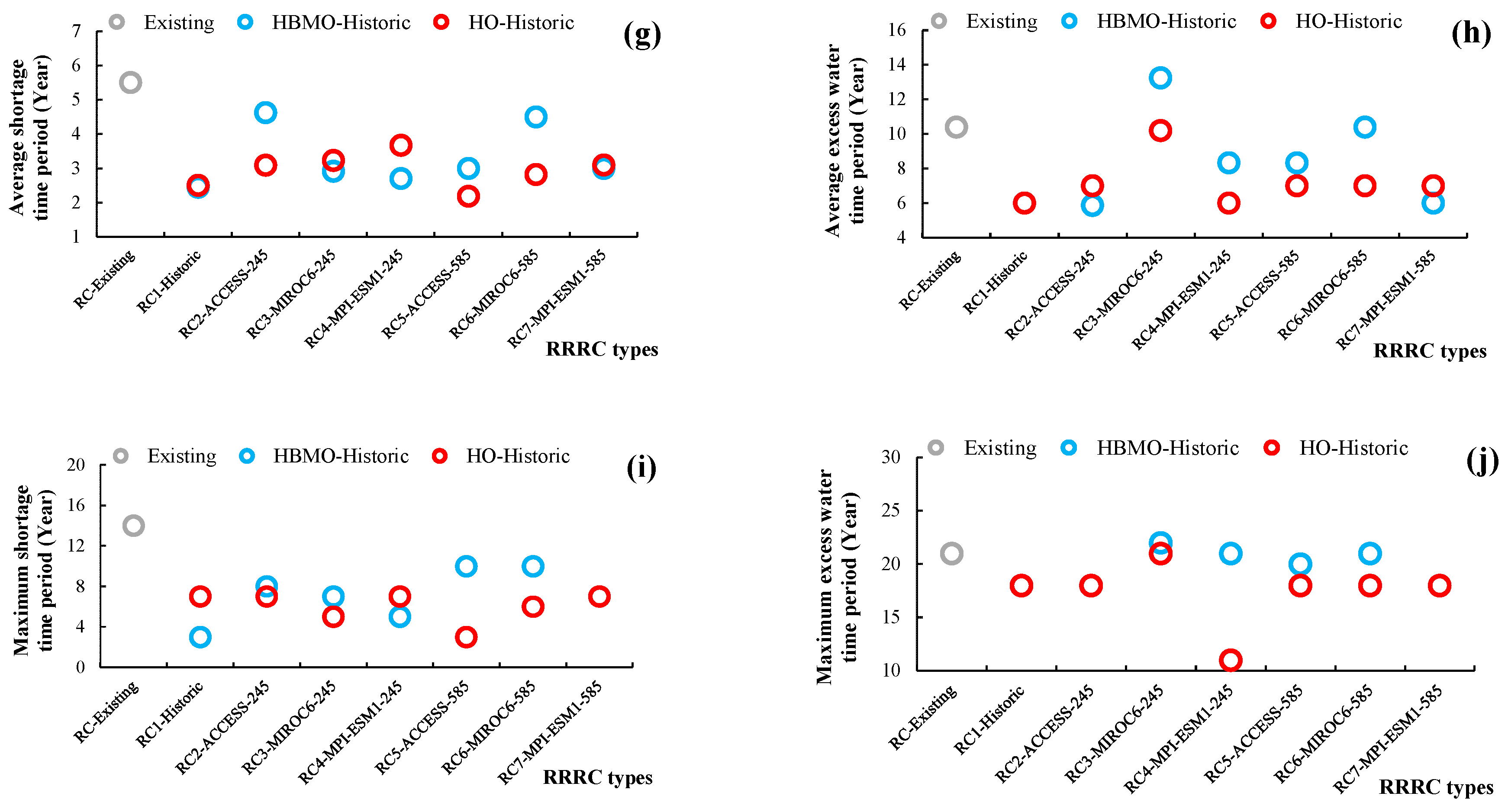
Table 1.
Data collected for WEAP and reservoir operation rule curve development by HO.
| No. | Data Type | Resolution | Year | Sources |
|---|---|---|---|---|
| 1 | Digital Elevation Model (DEM) | 30 × 30 m | 2017 | SRTM (Earth Resource Observation and Science (EROS) Center) |
| 2 | Land use | 30 x 30 m | 2019 | Land Development Department (LDD) |
| 3 | Soil group | 30 x 30 m | 2018 | Land Development Department (LDD) |
| 4 | Precipitation | Daily | 2000 – 2023 | Thai Meteorological Department (TMD) |
| 5 | Inflow in reservoir and storage capacity | Monthly | 2000 – 2023 | Electricity Generating Authority of Thailand (EGAT) |
| 6 | Evaporation | Monthly average | 2000 – 2023 | Royal Irrigation Department (RID) |
| 7 | Allocated water from downstream | Monthly average | 2000 – 2023 | Royal Irrigation Department (RID) |
Table 3.
Annual average precipitation.
| Scenarios | Periods/Years | Average | Range of 3 GCMs | ||
|---|---|---|---|---|---|
| (mm) | BL diff. (%) | Min. (mm) |
Max. (mm) |
||
| Baseline (BL) | 2000 - 2023 | 1,188.4 | - | - | - |
| SSP245 | 2024 - 2055 | 1,336.8 | 12.5 | 1,189.3 | 1,482.2 |
| SSP585 | 2024 - 2055 | 1,347.6 | 13.4 | 1,144.5 | 1,567.5 |
Table 4.
Annual average temperatures.
| Scenarios | Periods/Years | Average | Range of 3 GCMs | ||
|---|---|---|---|---|---|
| (°C) | BL diff. (°C) | Min. (°C) |
Max. (°C) |
||
| Baseline (BL) | 2000 - 2023 | 27.7 | - | - | - |
| SSP245 | 2024 - 2055 | 28.7 | 1.0 | 28.0 | 29.4 |
| SSP585 | 2024 - 2055 | 28.9 | 1.1 | 28.1 | 29.1 |
Table 5.
Performance ratings for evaluation metrics for a monthly time step [68].
Table 5.
Performance ratings for evaluation metrics for a monthly time step [68].
| Performance Rating | R2 | NSE | RSR | PBIAS |
|---|---|---|---|---|
| Very Good | 0.75<R2≤1.00 | 0.75<NSE≤1.00 | 0.00<RSR≤0.50 | PBIAS<±10 |
| Good | 0.65< R2≤0.75 | 0.65<NSE≤0.75 | 0.50<RSR≤0.60 | ±10≤ PBIAS<±15 |
| Satisfactory | 0.50< R2≤0.65 | 0.50<NSE≤0.65 | 0.60<RSR≤0.70 | ±15≤ PBIAS<±25 |
| Unsatisfactory | R2≤0.50 | NSE≤0.50 | RSR>0.70 | PBIAS≥±25 |
Table 6.
Optimal parameters for study area from WEAP calibration.
| No. | Parameters | Land use | |||||
|---|---|---|---|---|---|---|---|
| Agriculture | Forest | Urban | Shrubland | Wetland | Water | ||
| 1 | Crop coefficient (Kc) | 0.88 | 1.04 | 0.40 | 0.80 | 0.80 | 0.80 |
| 2 | Soil water capacity (SWC, mm) | 500.0 | 1000.0 | 50.0 | 300.0 | 700.0 | 600.0 |
| 3 | Deep water capacity (DWC, mm) | 1,000.0 | 1,000.0 | 1,000.0 | 1,000.0 | 1,000.0 | 1,000.0 |
| 4 | Runoff resistance factor (RRF) | 2.0 | 0.2 | 4.0 | 0.5 | 1.5 | 1.0 |
| 5 | Root zone conductivity (RZC, mm/month) | 20.0 | 20.0 | 20.0 | 20.0 | 20.0 | 20.0 |
| 6 | Deep conductivity (DC, mm/month) | 20.0 | 20.0 | 20.0 | 20.0 | 20.0 | 20.0 |
| 7 | Preferred flow direction (PFD) | 0.15 | 0.15 | 0.15 | 0.15 | 0.15 | 0.15 |
Table 7.
Evaluation result of precision between calculation by WEAP and measured data.
| Items | Modeling stage | Evaluation statistics | |||
|---|---|---|---|---|---|
| R2 | NSE | RSR | PBIAS | ||
| Inflow | Calibration (2000-2011) | 0.86 | 0.84 | 0.40 | -13.68 |
| Validation (2012-2023) | 0.82 | 0.79 | 0.46 | 4.41 | |
| Overall (2000-2023) | 0.84 | 0.82 | 0.43 | -5.20 | |
| Storage volume | Calibration (2000-2011) | 0.55 | 0.52 | 0.69 | -6.77 |
| Validation (2012-2023) | 0.78 | 0.76 | 0.49 | 5.74 | |
| Overall (2000-2023) | 0.66 | 0.66 | 0.58 | -0.66 | |
Table 8.
Monthly average of Ubolrat Reservoir inflow for each scenario (Unit: MCM).
| Month | Baseline (2000-2023) |
Future (2024-2055) | |||||||
|---|---|---|---|---|---|---|---|---|---|
| ACCESS-CM2 | MIROC6 | MPI-ESM1-2-LR | Average of 3 model | ||||||
| SSP245 | SSP585 | SSP245 | SSP585 | SSP245 | SSP585 | SSP245 | SSP585 | ||
| Jan | 14.7 | 38.6 | 41.7 | 32.7 | 40.1 | 39.7 | 36.8 | 37.0 | 39.5 |
| Feb | 14.2 | 39.9 | 42.6 | 49.3 | 49.0 | 43.2 | 58.9 | 44.1 | 50.2 |
| Mar | 27.2 | 58.3 | 71.9 | 52.7 | 65.6 | 49.1 | 66.9 | 53.3 | 68.1 |
| Apr | 50.3 | 93.2 | 129.9 | 102.6 | 118.6 | 94.4 | 126.7 | 96.7 | 125.0 |
| May | 135.5 | 236.3 | 292.2 | 286.1 | 327.7 | 269.8 | 260.7 | 264.1 | 293.6 |
| Jun | 157.3 | 338.1 | 342.3 | 408.7 | 462.4 | 317.7 | 332.5 | 354.8 | 379.0 |
| Jul | 221.9 | 444.4 | 346.9 | 538.0 | 625.9 | 440.4 | 444.0 | 474.3 | 472.2 |
| Aug | 421.1 | 676.5 | 567.6 | 822.7 | 775.9 | 636.0 | 720.6 | 711.7 | 688.1 |
| Sep | 851.5 | 987.2 | 990.9 | 879.1 | 919.4 | 1018.9 | 944.8 | 961.7 | 951.7 |
| Oct | 709.0 | 410.7 | 420.2 | 454.9 | 396.8 | 482.5 | 454.2 | 449.4 | 423.7 |
| Nov | 179.6 | 49.8 | 50.7 | 70.4 | 49.1 | 80.7 | 90.1 | 67.0 | 63.3 |
| Dec | 28.6 | 28.6 | 29.3 | 29.5 | 29.4 | 29.0 | 28.9 | 29.0 | 29.2 |
| Annual | 2,811.0 | 3,401.5 | 3,326.3 | 3,726.7 | 3,860.0 | 3,501.2 | 3,565.1 | 3,543.1 | 3,583.8 |
| Baseline difference | +21.0% | +18.3% | +32.6% | +37.3% | 24.5% | 26.8% | 26.9% | 27.5% | |
Table 9.
Comparison of the maximum efficiency of RRRC-HO with existing rule curve and HBMO.
| Testing scenarios | Historic inflow |
SSP245 inflow |
SSP585 inflow |
Best RRRC | HO vs. HBMO |
|---|---|---|---|---|---|
| Water shortage | |||||
| Frequency (times per year) | 0.786 ⟶ 0.429 (45%) | 0.645 ⟶ 0.032 (95%) | 0.645 ⟶ 0.065 (90%) | RC2, RC5, RC7 | HO ≤ HBMO Lower |
| Average shortage (MCM) | 242.55 ⟶ 122.29 (50%) | 96.39 ⟶ 4.00 (96%) | 89.26 ⟶ 1.74 (98%) | RC1, RC2, RC5 | HO ≤ HBMO Lower |
| Maximum shortage (MCM) | 942 ⟶ 810 (14%) | 549 ⟶ 13 (98%) |
343 ⟶ 54 (84%) |
RC5, RC6 | HO ≈ HBMO Range |
| Average duration (year) | 5.5 ⟶ 2.2 (60%) |
3.3 ⟶ 1.0 (70%) |
4.0 ⟶ 1.0 (75%) |
RC5, RC7 | HO ≤ HBMO Lower |
| Maximum duration (year) | 14 ⟶ 3 (79%) |
6 ⟶ 1 (83%) |
8 ⟶ 1 (88%) |
RC5, RC7 | HO ≤ HBMO Lower |
| Excess water | |||||
| Frequency (times per year) | 0.929 ⟶ 0.857 (8%) | 1.0 ⟶ 1.0 (0%) |
1.0 ⟶ 1.0 (0%) |
RC1, RC4 | HO ≈ HBMO |
| Average shortage (MCM) | 1,346 ⟶ 1,200 (11%) | 2,103 ⟶ 1,958 (7%) | 1,992 ⟶ 1,829 (8%) | RC1, RC3, RC5 | HO ≤ HBMO Lower |
| Maximum shortage (MCM) | 4,139 ⟶ 4,100 (1%) | 3,652 ⟶ 3,340 (9%) | 4,222 ⟶ 3,872 (8%) | RC1, RC5 | HO ≈ HBMO Range |
| Average duration (year) | 10.4 ⟶ 6.0 (42%) | 31 ⟶ 31 (0%) |
31 ⟶ 31 (0%) |
RC1, RC4 | HO ≈ HBMO |
| Maximum duration (year) | 21 ⟶ 11 (48%) |
31 ⟶ 31 (0%) |
31 ⟶ 31 (0%) |
RC4 | HO ≈ HBMO |
Disclaimer/Publisher’s Note: The statements, opinions and data contained in all publications are solely those of the individual author(s) and contributor(s) and not of MDPI and/or the editor(s). MDPI and/or the editor(s) disclaim responsibility for any injury to people or property resulting from any ideas, methods, instructions or products referred to in the content. |
© 2026 by the authors. Licensee MDPI, Basel, Switzerland. This article is an open access article distributed under the terms and conditions of the Creative Commons Attribution (CC BY) license (http://creativecommons.org/licenses/by/4.0/).
Copyright: This open access article is published under a Creative Commons CC BY 4.0 license, which permit the free download, distribution, and reuse, provided that the author and preprint are cited in any reuse.


