
Submitted:
22 December 2025
Posted:
25 December 2025
You are already at the latest version
Abstract
Cyclic freezing and thawing of concrete specimens are one of the main causes of cracking in concrete. Current procedures for assessing frost resistance of concrete in Germany rely mainly on the CIF and CDF tests that utilise qualitative estimation of cracks. Although these standard tests provide a general overview of the condition of concrete damage through the estimation of water saturation through capillary suction, mass of surface delamination, qualitative open surface damage, and relative dynamic modulus of elasticity, they do not take quantitative analysis of cracks directly into account. To facilitate this quantitative approach, cracks are studied in concrete samples exposed to specific standard cycles of freezing and thawing, then scanned using micro computed tomographic (µCT) imaging, and consequently cut for petrographic thin section analysis. The thin sections are scanned using light microscopy (LM). Deep learning frameworks were deployed to train semantic segmentation models to identify cracks, air pores, aggregate, and cement matrix. Both scanned modalities were co-registered using three experimental variations of varying processing complexity that rely on matching of Fourier-based shape descriptors and underlying features thereof to verify and validate the quality of segmentation inferred for various phases of concrete.
Keywords:
semantic segmentation
; cracks analysis
; slice-to-volume registration
; Fourier descriptors
; features matching
; spherical harmonics analysis
1. Introduction
1.1. Background and Motivation
Cyclic freezing and thawing (FT) can critically affect concrete, causing internal damage that leads to cracking, flaking, and settling, which reduce the durability and serviceability of concrete elements, especially in cold regions [1]. Cracking may occur when water is absorbed into the voids of concrete, a heterogeneous multiphase composite porous material, causing internal pressure forces to build up as it freezes, due to the volume expansion of freezing water up to around 9% [2], exerting expansive forces beyond its tensile strength [3].
Air voids of hydrated cement, including pores and cracks, may exist within a continuous range of sizes from nano- to micrometres. Pores are contained in both the calcium silicate hydrate gel phase of the cement paste and in capillary pores occurring in remnants of space previously occupied by mixing water [4]. While cracking in concrete is consequently affected by the long-term conditions to which the concrete element is subjected, long-term exposure and loading extend in most cases the magnitude of cracks, principally their width, in both reinforced and plain concrete [5]. Chemical and physical reactions within the concrete are further influenced by moisture uptake transferred through these pores and cracks.
While currently adopted test procedures show that qualitative rating in microscopic analysis is still applied to assess crack damages for shrinkage [6], quantification ensures better reproducibility that could apply to computed tomographic scans as well [7,8]. For reliable quantification of internal damage due to freezing and thawing, Grattan-Bellew et al. [9,10] proposed the Damage Rating Index method (DRI), a semi-quantitative microscopic tool used to appraise damage in concrete relying on petrographic analysis. Distress features are counted in cm squares drawn on the surface of polished concrete sections using a stereomicroscope at 15-16× magnification [11]. The damage features are then multiplied by weighting factors whose purpose is to balance their relative importance towards the corresponding distress mechanism (e.g., Alkali-silica reaction (ASR)), as proposed by Villeneuve and Fournier [12]. The DRI number is therefore calculated and assessed over a sufficiently representative surface area of at least 200 , then normalised to a 100 area, where the higher the DRI number, the higher the damage degree [13] is.
Martin et al. [14] established a fairly good agreement in the testing procedures of the of the DRI to the Stiffness Damage Test (SDT), and Residual Expansion (RE). Such correlation of the DRI is further investigated by Sanchez et al. [15] to assess the condition of concrete affected by internal swelling reaction (ISR) mechanisms (i.e., ASR, delayed ettringite formation and freeze-thaw cycles), to verify the suitability of the DRI for becoming a comprehensive damage evaluation protocol. The DRI was found to enable a quantitative damage evaluation for concrete, regardless of the distress mechanism type and degree. Moreover, their implementation of an extended DRI version makes the method more suitable to describe progress of different ISR deterioration processes in concrete.
Although the DRI has been increasingly used in North America [15], the standardised German procedures for measuring the resistance to freezing and thawing [16] are mainly the Capillary de-icing freeze-thaw (CDF) [17] and Capillary suction, Internal damage and Freeze-thaw (CIF) [18] tests. The CDF test determines the amount of scaled material and the mass of solution sucked up during the capillary suction period for each specimen at least after 14 and 28 FT cycles. For the CIF test, the following sequence of measurements is imperative for estimating the relative dynamic modulus of elasticity for the specimen: (1) surface scaling, (2) water uptake, (3) internal damage through estimating the relative ultrasonic transit time (i.e., reference method) or through measuring fundamental transverse frequencies or length change as alternative methods.
Laboratory-scale methods, such as ultrasonic pulse transmission time and fundamental transverse frequency measurements, as specified in CDF/CIF, can directly evaluate internal FT damage. These methods assess FT resistance by comparing data before and after FT exposure and have varying conditions and tested values in various standards [19]. Therefore, for in-situ assessments, these methods cannot provide a quantitative description of FT damage to the structure. This implies that indirect estimation methods are necessary for the in situ assessment of concrete structures [20].
The limitations to the use of CDF/CIF tests include: (a) not taking into account the change and complexity of the air-void system characteristics due to capillary porosity and cracks connectivity networks formed in concrete, which affect its capillary suction of surface liquid under freezing and their relationship with scaling, moisture uptake, and mass loss, that vary based on the unique properties and type of the concrete tested [21], (b) the main initial temperature and moisture conditions of the concrete outdoors prior to conducting the FT testing, which may not accurately reflect the actual moisture and ice formation within the material in its intended use. It can overestimate the effect of freeze-thaw cycles and may not be applicable to all types of concrete [22], (c) measuring internal damage can be complex and may not always provide a clear picture of the overall frost resistance that can be influenced by various extrinsic factors environmental and structural [23], or by testing protocol, other intrinsic factors affecting the specific mixture of concrete, like cement type, water-cement ratio and the sturdiness of aggregates used [3], (d) the effect of concrete additives, their dosages, optimal external conditions for appropriate usage, and the influence of these variables on current testing procedures used to enhance concrete freeze-thaw durability through different mechanisms are under-investigated in the body of literature, where four mechanisms contributing to frost resistance are mainly deployed, be it by providing extra space for ice expansion in concrete using air bubbles, reducing the porosity of concrete using pozzolans and fillers, containing crack propagation using microfibres, nanotubes and nano-sheets, and decreasing water absorption using hydrophobic agents [24], and (e) the results might not always correlate well with the actual performance of the material in the field or can overestimate the effect of FT cycles and may not be applicable to all types of concrete. While these tests offer valuable insights into frost resistance, they may not always correlate to the actual freezing and thawing conditions the concrete is exposed to nor accurately reflect the real-world behaviour of the concrete on site [25] and may not be applicable to all types of concrete, especially non-standard mixtures with additives.
These limitations increase the need for a reliable automated method to quantify cracks for FT damage assessment procedures. However, the automated detection of cracks in computed tomographic scans of concrete specimens is a difficult task. State of the art solutions to cracks segmentation rely heavily on machine or deep learning methods for pixel-wise classification in images. However those methods are limited to the specifications and maximal resolution of the scanning device used, which constrains the ability to detect features beyond the maximum resolution of the scanner for computed tomographic imaging (i.e., minimal widths of approximately 0.05 mm for crack width detectability in the cross-sectional image and 0.1 mm crack width measurability [8]). However, segmenting cracks to achieve a reliable pixel-wise classification of all features in a 2D computed tomographic image or a 3D images stack of 2D sections still lags behind in the body of literature mainly due to various factors [26] including (a) limitations to data availability, quality of training data and published annotated ground truths, (b) the inherent morphological features of cracks as single or multiple thinly jagged poly-lines with irregular varying widths that could exist as singular or multiple instances, interconnected and intersecting, branching out or extending to merge into other features like air pores or background, (c) the heterogeneous properties of concrete per se, which contain weak contrast air voids like cracks and air pores alongside varying density ingredients of the concrete (i.e., cement, aggregates, and admixtures), that are consequently limited to a greyscale intensity representation of the CT imaging modality representing the amounts of attenuation determined by the density of concrete matrix subcomponents and air voids in Hounsfield Units (HU), (d) the common occurrence of artefacts in computed tomographic images that degrade the image quality differently like ring and beam hardening artefacts, including cupping, streak and dark bands, metal or high density material artefacts, etc.
1.2. Objectives
The main objective of this research is to establish a reliable workflow to register arbitrary 2D LM slices to their corresponding slices in a 3D CT stacked model. We further analyse the registered output quantitatively to establish the difference in concrete phases and internal structural damage of specimens through a combined 2D and 3D imaging approach, focusing particularly on cracks and pores that affect moisture transfer and chemical reactions.
We prepare a dataset of 2D and 3D scans of cylindrical concrete specimens of standard DIN mixture to retrain deep learning frameworks for semantic segmentation. The compiled dataset employed micro-computed tomography (CT) 3D scans on cylindrical specimens and transmitted light microscopy of petrographic thin sections thereof. Additionally, we register the 2D thin sections within 3D volumes to quantitatively analyse the specimen’s porosity and cracks’ dimensions, while establishing correlations between 2D and 3D data to validate estimated quantification and lay the groundwork for improving the quality of cracks’ segmentation through data fusion in future work.
2. Related Work
2.1. Cracks Segmentation in 2D
The traditional approach that predates state-of-the art methods used crack detection and segmentation relied heavily on image processing techniques of which the review conducted by Zakeri et al. for image-based techniques for crack detection, classification and quantification in asphalt pavements [27], while Mohan et al. [28] compiled a collective review concisely explaining those various image processing techniques used in engineering structures mainly of concrete and to a lesser extent of steel.
2.1.1. Classical Image Processing Methods
Nazaryan et al. relied on the centre of gravity (i.e., centroid) of the images’ area to calculate the width and depth of cracks [29]. Meanwhile, anisotropic diffusion filtering at the pixel level was implemented in [30,31] to smooth out noise and artefacts in the background whilst preserving the crack defect contours; thus, improving the segmentation of cracks from a system of images. The load differential method developed by Chen et al. [32] resorted to comparing ultrasonic guided wave signals under the same damage state independent of past recorded damage free data to avoid baseline subtraction under mismatched conditions. The Digital Image Correlation (DIC) method utilised in [33,34,35,36] identified each pixel in a subsequent set of images by examining its neighbouring pixels to measure the full-field strains and displacement of loaded three dimensional objects in addition to visualising the resulting defects.
Gunkel et al. [37] developed a package written in R that allowed cracks detection and statistical analysis of their quantities using a shortest path algorithm, where crack clusters were predicted from connected components of pixels given a minimum threshold value, then the cracks’ paths were determined by Dijkstra’s algorithm. Image based multi-directional crack detection approach utilising Gabor filter was proposed by Glud et al. [38] requiring 5 user-inputs that are dependent on human visual apprehension. The Fast Discrete Curvelet Transform (FDCT) was first utilised in low contrast and dark coloured images along with texture analysis using the Grey Level Co-occurrence Matrix (GLCM) [39] to automatically detect cracks. GLCM was also implemented in [40] in combination with an Artificial Neural Network (ANN) classifier to estimate the cracks’ length and width.
Abdel-Qader et al. [41] compared the effectiveness of four edge detection algorithms on crack images of a bridge surface by using Fast Fourier Transform (FFT), Sobel filter, Fast Haar Transform (FHT) and Canny filter. The FHT is relatively new but it was shown to be significantly more reliable than the other three edge-detection techniques in identifying cracks. FHT transform decomposes the image into low-frequency and high-frequency components. This process is followed by isolating those high-frequency coefficients from which the edge features of an image are identified.
2.1.2. Machine Learning Methods
Rapidly advancing approaches for crack detection using machine learning methods have gained more popularity with deep learning, where their outstanding results compared to some of the aforementioned methods [42] outperform the preceding traditional methods [43]. Dorafshan et al. evaluated the performance of six edge detectors (i.e., Roberts, Prewitts, Sobel, Laplacian of Gaussian (LoG) in spatial domain, and both Butterworth and Gaussian filters in frequency domain) and compared them to the performance of a fully trained AlexNet convolutional neural network (CNN) concluding superior results to the latter and further proposed a hybrid detector in which sub-images were first labelled by a trained CNN then LoG edge detector was only applied on the sub-images identified to reduce the noise ratio [44].
Zhang et al. [45] proposed a CNN model for binary classification of image patches containing cracks leveraging deep learning based detectors that was successfully applied to images with complex background captured using a smartphone. Xu et al. [46] proposed another CNN structure based on a Restricted Boltzmann Machine (RBM) encoder for crack identification and extraction of comprising image windows containing cracks with a complex background. Fan et al. proposed another CNN structure for classifying crack images in addition to an adaptive thresholding method by searching for a threshold along the principal diagonal of the 2D histogram that stores the intensity of each pixel and the mean intensity of its neighbourhood using k-mean clustering [47].
The DeepCrack implementation by Zou et al. returned results for multiple scales of the input, which were eventually fused in a 1 x 1 convolutional layer, where both an encoder and a decoder contributed to scales corresponding to the pooling or deconvolutional stage respectively and the cross-entropy loss was adapted to incorporate losses on individual scale levels [48]. Comparably, the CNN model proposed by Liu et al. [49] for a CNN named DeepCrack computed the cross-entropy loss on the side-outputs of each scaled level then applied conditional random fields and guided filtering to reach a fused ground truth with no explicit decoder learned.
Benz et al. [50] presented an expanded approach by applying transfer learning for crack segmentation on the model of TernausNet [51] that is based on the architecture of the UNet. The implemented CNN named CrackNausNet could learn separate representations of crack and planking by introducing a third class for planking patterns.
Kang et al. [52] proposed a crack detection, localisation and quantification method utilising a three step algorithm. First, a faster proposal region convolutional neural network (Faster R-CNN) was used to detect crack regions. The network contained two different networks: a Region Proposal Network (RPN) and a fast region-based convolutional network (Fast R-CNN) [53]. The RPN provided possible object locations using various bounding box sizes, and as a classifier, the Fast R-CNN proposed the probability of the object. Then, the determined windows were inputted into the modified Tubularity Flow Field (TuFF) [54] algorithm for crack segmentation at the pixel level. Finally, the segmented cracks were processed by the modified Distance Transform Method (DTM) to measure their thicknesses and lengths.
2.2. Cracks Segmentation in 3D
Barisin et al. [26] summarised the latest developments in the body of literature and state of the art methods adopted for the 3D semantic segmentation of cracks in CT scans. The authors highlighted relevant technical challenges of the task as elaborated in Section 1.1 and the classical methods used for CT scans segmentation of cracks [55].
Tree-based methods can be used initially to segment 2D images. Random forests have been specifically proven to be an appropriate tool to segment 2D images of concrete [56,57]. A generalisation to 3D is straightforward, where the random forest, as a collection of decision trees, each trained on several feature grey values of voxels of the original image and/or of several image transforms. Each tree is in turn trained on a different training dataset obtained by using the bootstrap procedure on the original training data. For every tree, the feature vectors are drawn randomly and with replacement until the size of the original training dataset is reached. The output of a decision tree is a classification of the voxel as crack or no crack (i.e., 1 or 0 respectively). As the classifications of the single trees may differ, the final prediction is obtained via majority voting. The main parameters of the method are the depth of the trees and the maximum number of trees. Additionally, the parameters of the image transforms used for constructing the features have to be chosen [26].
Patzelt et al. [8] utilised a semi-automated approach for segmenting CT images by training a multi-class classifier using features extracted automatically from Gaussian blur, Hessian, Derivatives, and Laplacian filters, as well as Edges using gradient magnitude computation, suppression of locally non-maximum gradient magnitudes, and hysteresis thresholding, difference of Gaussian, minimum, maximum, mean, variance, and median voxel values within a specified kernel size [58]. Although the authors demonstrated the feasibility of unsupervised machine learning algorithms for the cracks segmentation task, the difference in area of segmented cracks between manually coregistred CT and light microscopy scans was significantly high at around 14.42%.
To eliminate the need for labour-intensive pixel-annotation of the images, unsupervised semantic segmentation offers an alternative solution. Sadrnia et al. [59] selected two state-of-the-art frameworks, Self-supervised Transformer with Energy-based Graph Optimization (STEGO) [60] and Eigen Aggregation Learning (EAGLE) [61], due to their success on benchmarks, were retrained on the CT [62] and DeepCrack [49] datasets. The quantitative results of STEGO trained on CT are promising, but the qualitative results show that it failed to detect cracks, whereas EAGLE with nearly identical metrics could partially detect cracks, when class imbalances are not addressed. Based on the qualitative results on DeepCrack, both models detected cracks in this dataset, however, EAGLE performed worse than STEGO in metrics, including score and mean intersection over Union (mIoU).
3D UNet [63] is a supervised learning framework introduced originally for biomedical image segmentation tasks. It is a convolutional neural network with characteristic u-shape of the original 2D UNet architecture [64] resulting from a composition into encoder and decoder. The encoder is responsible for capturing the image context. Then, the decoder expands the downsampled feature map back to the original image size. In order to prevent overfitting, [55] introduced a layer with a dropout probability of 0.5 between the decoder and encoder bottleneck. The output of the network is a probability map of the same size as the input image valued in-between , where the probabilities for each voxel are whether it belongs to a specific class (e.g., crack) or not. The binary image is obtained through thresholding.
Barisin et al. [26] trained a modified Deep Neural Network called RieszNet, built from layers consisting of transformation batch normalisation, Riesz layer, and rectified linear unit (ReLU). Batch normalisation improved the training capabilities and avoided overfitting, while ReLUs introduced nonlinearity to the model. The Riesz layer extracted scale equivariant spatial features using a linear combination of first and second order Riesz transform [65] in 3D and generalized well on unseen data after training in comparison to Fine-tuned multi-scale variation of 3D UNet [66].
2.3. Shape Description and Registration
Brandstätter et al. [67] developed a pipeline to register 2D slices (i.e., source) to a 3D stack of computed tomographic slices (i.e., target) using extracted 2D patches sampled into 2D planes orthogonal to the normal vectors to the Hilbert surface of its 3D sub-volume, then passing passed the patches into a rotation equivariant ResNet (ReResNet) model to generate normalised features that could be queried to identify the closest neighbour volume feature based on the distance between source and target feature vectors. The Random Consensus (RANSAC) is consequently used to estimate a 3D affine pose transformation to the slice in 3D space. The main limitation to this pipeline is the rigidity of registration as well as scaling and translation dependency.
Al-Thelaya et al. developed a framework for generating 2/3D invariant shape descriptors (InShaDe) [68] for 2D closed contours and 3D watertight mesh closed surfaces respectively, mainly applied on shape analysis and classification of histology image shapes (e.g., cell walls). The generate a 2D descriptor, the contour is preprocessed through iterative smoothing and resampling algorithm to fix the contour’s dimensionality relying on Nyquist frequency sampling constraint [69]. The 2D shape descriptor could then be calculated based on sparse encoding the discrete curvatures and the lowest energy coefficients thereof derived from elliptic Fourier analysis. For 3D shapes, the descriptor is generated based on discrete mean curvature and spherical harmonics decomposition using Willmore gradient flow parametrisation [70] to calculate the invariant energy coefficients.
3. Materials and Methods
3.1. Materials and Specimens Preparation
We use concrete cylindrical specimens of height and diameter of 75 mm and 50 mm respectively. The cylindrical shape was selected to ensure uniform irradiation of the rotating specimen and thus reduce physically induced artefacts formation around the edges of the 3D dataset. For that purpose, 3D-printed moulds were additively manufactured using an extrusion-based printing with a Fused Filament Fabrication (FFF) 3D printer and Polylactic Acid (PLA). After 28 days of storage under standardised conditions (DIN EN 12390-2), the samples were exposed to several freeze-thaw cycles (i.e., CIF test). Basic requirement for the generation of cracks was that the mixture recipe had sufficient sensitivity resistance to freeze-thaw stress and at the same time low-shrinkage behaviour.
The specimens obtained from frost-damaged and mechanically stressed concrete are prepared petrographic analysis by impregnation with a yellow epoxy resin under vacuum to enhance the contrast between the voids and other phases of the concrete. Three thin sections are cut from the specimens along the central axial plane and two further sections on the left and right of it targeting a thickness of approximately for each slice.
3.2. Data Acquisition
We generate a 3D dataset of six high resolution computed tomographic (CT) scans using the “GE Phoenix Nanotom M research | edition”, a micro and nano CT system equipped with a high-power nanofocus X-ray tube and an internally cooled detector, with targeted voxel size for the scans of approximately and resolution of . The 2D dataset of light microscopy scans from petrographic thin sections are acquired using a high-resolution transmitted-light scanner “Microtek, Scanmaker 4800” with a resolution pixel size of .
3.3. Methods
3.4. Beam Hardening Correction in CT Scans
To remove beam hardening artefacts, we develop a workflow summarised in Figure 1 to process 3D CT scans comprising of a stack of 2D slices. The colour value at each pixel of the greyscale image is considered as a third dimension orthogonal to the slice. The slices are converted into 8 Bits to reduce the time and memory size needed for processing and then denoised using non-local means algorithm to preserve their texture. We then threshold the 2D slices using mean shift and define the background by retrieving the cluster of the lowest mean colour intensity value. The background is then set to black and white then smoothed using a Gaussian blurring filter to neutralise the original background colour bleeding into the foreground of the specimen. An equal weighted sum of the two images produces a smoothed out image with no sharp features that could be used to efficiently estimate the beam hardening effect by inverting the output mask’s and fitting its foreground to that of the denoised slice on each slice separately or alternatively for the whole 3D stack using Least Mean Square (LMS) Regression with the objective function optimising the colour value difference to be minimum. The optimal height is then subtracted from the output mask to generate an inverted filter of the beam hardening effect. Subtracting the filter from the original slice image produces a slice free of beam hardening artefacts after denoising it with edge-preserving bilateral noise filtering and Contrast Limited Adaptive Histogram Equalisation (CLAHE) [71] as demonstrated in the last sub-figure of Figure 1. Figure 2 shows a comparison on circular and square cross-section slice prior and post beam hardening correction.
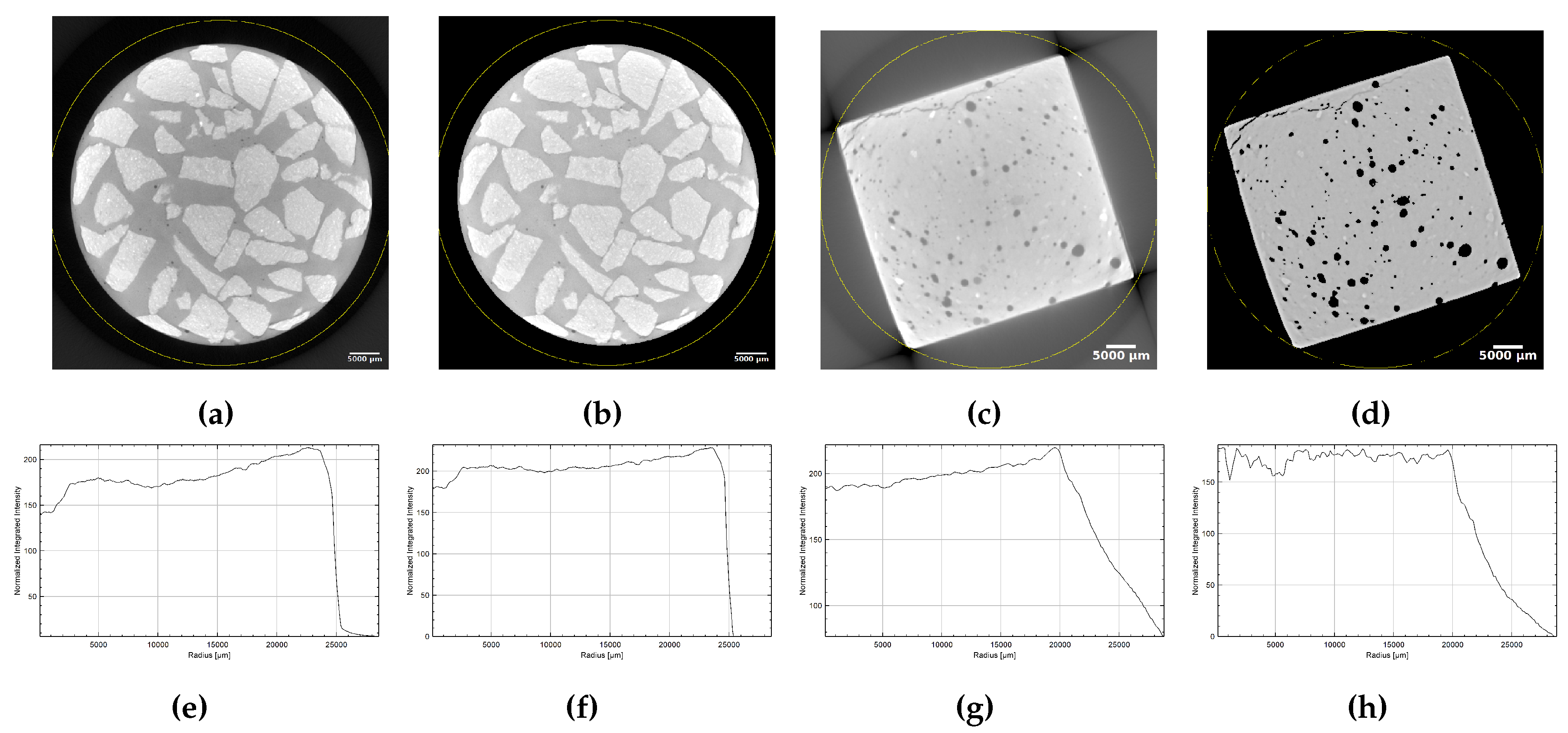
Figure 2.
CT slice prior and post beam hardening artefacts correction of circular and squared cross-section specimens. (a) Original slice of a cylindrical specimen with ROI concentric circle profile marked in yellow. (b) Corrected slice with same ROI profile marked in yellow. (c) Original slice of a cube specimen with ROI concentric circle profile marked in yellow. (d) Corrected slice with same ROI profile marked in yellow. (e) Profile plot of normalized integrated intensities around concentric circle before beam hardening correction of (a). (f) Profile plot of normalized integrated intensities around concentric circle after beam hardening correction of (b). (g) Profile plot of normalized integrated intensities around concentric circle before beam hardening correction of (c). (h) Profile plot of normalized integrated intensities around concentric circle after beam hardening correction of (d).
3.5. LM Semantic Segmentation
For semi-automatic annotation of the LM dataset, we preprocess the images using a two-step enhanced clustering approach through Uniform Manifold Approximation and Projection (UMAP) [72] technique first that can be used for general non-linear dimensionality reduction to model the Riemannian manifold of the data distribution with a fuzzy topological structure. The resulting embedding is found by searching for a low dimensional projection of the data that has the closest possible equivalent fuzzy topological structure and can be used in the second step for clustering using Bayesian Gaussian Mixture [73,74] by aggregating sub-cluster embeddings together. The final annotation mask is then generated semi-automatically after patchifying large scans into smaller images and cleaning inaccuracies using automated annotation tool LabelMe [75] to assign the correct labels for classes. Figure 3 shows a sample of the process on a patch and a full petrographic scan, their intermediary clustering masks and the final annotation masks.
We compile an augmented dataset of 22,000 images and their respective annotation masks of resolution 256 × 256 pixels comprising the following 5 classes: background (B), cracks (C), aggregate (A), air pores (AP), and cement matrix (CM) to train a DNN for semantic segmentation. We retrain an Attention Residual UNet [76] in 16 batches for 200 epochs on an 80:20 % data split for training and validation respectively. The focal cross entropy is used as the loss function. The evaluation metrics selected for training are Accuracy, which is calculated by the number of correct predictions over a whole scene using the formula , and mean Intersection over Union (mIoU), which estimates the overlap between the ground truth and the prediction over the union of the sample sets using the formula , such that TP, TN, FP and FN are the number of True Positive, True Negative, False Positive and False Negative values respectively. The learning curves in Figure 4(a), (b) illustrate the model’s accuracy and loss performance on the training and validation sets respectively, whereas Figure 4(c) illustrates the inference performance of the network on some validation samples. The trained model evaluation reached an Accuracy and mean of 98.516% and 83.591% respectively on the validation dataset. We apply a sliding window subdivision patching for inference on large images with half patch-size overlap and Gaussian patch centre weighting to predict smooth segmentation masks to minimise visible stitching artefacts and Field of View mislabelling limitations around the borders.
3.6. CT Semantic Segmentation
We segment the beam hardening corrected CT scans, after denoising through Swin-Conv-UNet (SCUNet) [77], using heuristic image processing and enhanced clustering analogous to the process in Section 3.5 into 4 classes: cracks, air pores, cement matrix and aggregates, when aggregates are of recognisably different density than that of the cement matrix. The output segmentation masks were then further processed by manually adjusting and correcting mislabelled annotations through the Computer Vision Annotation Tool (CVAT) [78]. At unrecognisable colour intensity values of aggregates from cement matrix due to similar densities, aggregate’s binary annotation masks required for binary segmentation were generated semi-automatically using Meta’s Segment Anything Model (SAM) [79] and Labelme [75]. Figure 5 shows the outputs of the intermediary steps to create the annotation masks. Relatively successful attempts to use 2D unsupervised semantic segmentation via STEGO [60] and EAGLE [61], summarised in [59], have been made albeit with a meticulous weight balancing of classes during augmentation. For segmenting the four classes, we trained a 2D semantic segmentation Attention Residual UNet [76] on 11,000 images of 128×128 pixels with 85:15% data split in 8 batches from the annotation masks generated by the first approach for 100 epochs. Similar to LM segmentation, the focal cross entropy loss function for training, as well as Accuracy and mIoU for the evaluation metrics were used. The trained model evaluation reached an Accuracy and mean of 97.253% and 67.942% respectively on the validation dataset. In specimens where the aggregate density is similar to intensity values range of cement matrix, the Attention Residual UNet performed poorly on aggregates when the density of aggregate cement matrix was similar and failed to generalise on the validation dataset. Hence, we pivoted to binary segmentation of aggregates separately by deploying Cellpose [80].
The detailed evaluation results for the trained STEGO and EAGLE networks are elaborated in [59], whereas Figure 6 shows the learning curves for the Attention Residual UNet retrained for semantic segmentation of cracks, air pores, aggregate and cement matrix and compares its performance with inference samples from our trained unsupervised segmentation models STEGO and EAGLE.
3.7. Post-Processing and Shape Descriptors Generation
We extract and study morphological shape instances of the segmented concrete phases and their characteristic features from the prediction masks of Cracks, Aggregates, Air pores within the 2D and 3D datasets identified as possibly distinctive enough to match features for non-rigid registration. Furthermore, we consider normalisation methods to generate scale, rotation, reflection and translation invariant descriptors.
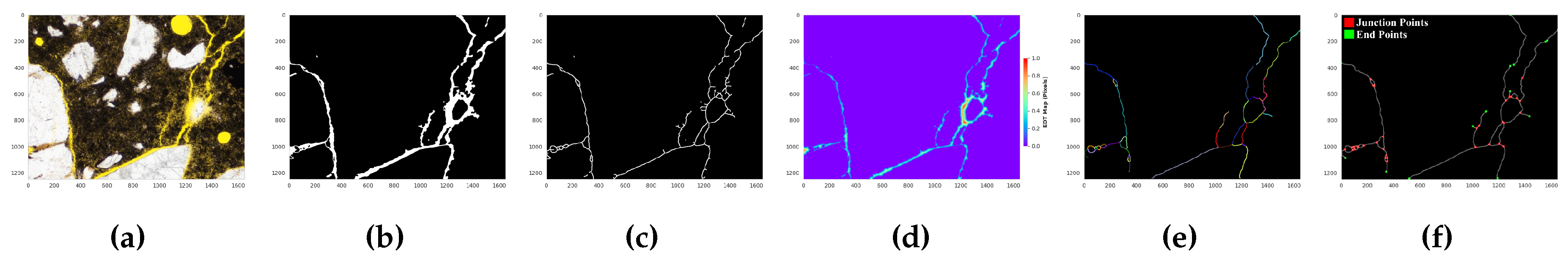
Cracks prediction masks are used to generate 2D/3D skeletons using Kimimaro library [81], based on a modified tree-structure extraction algorithm delivering skeletons that are accurate and robust (TEASAR) [82], and Euclidean distance transform (EDT) maps to estimate their widths and to calculate Compressed Sparse Row (CSR) pixel graph of its morphological skeletons using Skeleton Analysis [83]. To remove skeletonisation artefacts, we filter out branches of lengths smaller than the calculated width of the crack based on the previously calculated widths’ map. We then extract 2D junction points of cracks and reconstruct the main branches cleared of artefacts into their respective edges in the 3D stack.
Figure 7.
Visual example for extraction of relevant cracks point sets namely junction points and end points, and normalised feature thereat. The same principles apply in 3D with extension in z dimension. (a) original RGB LM patch of a larger scan. (b) Binary mask for cracks after removing salt and pepper noise. (c) Morphological skeleton of the binary mask using Guo-Hall thinning algorithm. (d) Normalised Euclidean Distance Transform (EDT) map. (e) Cracks main branches labelled with random colours after filtering secondary branching skeletonisation artefacts less than cracks’ widths. (f) Detected junction and end points from traversing the pixel graph in (e).
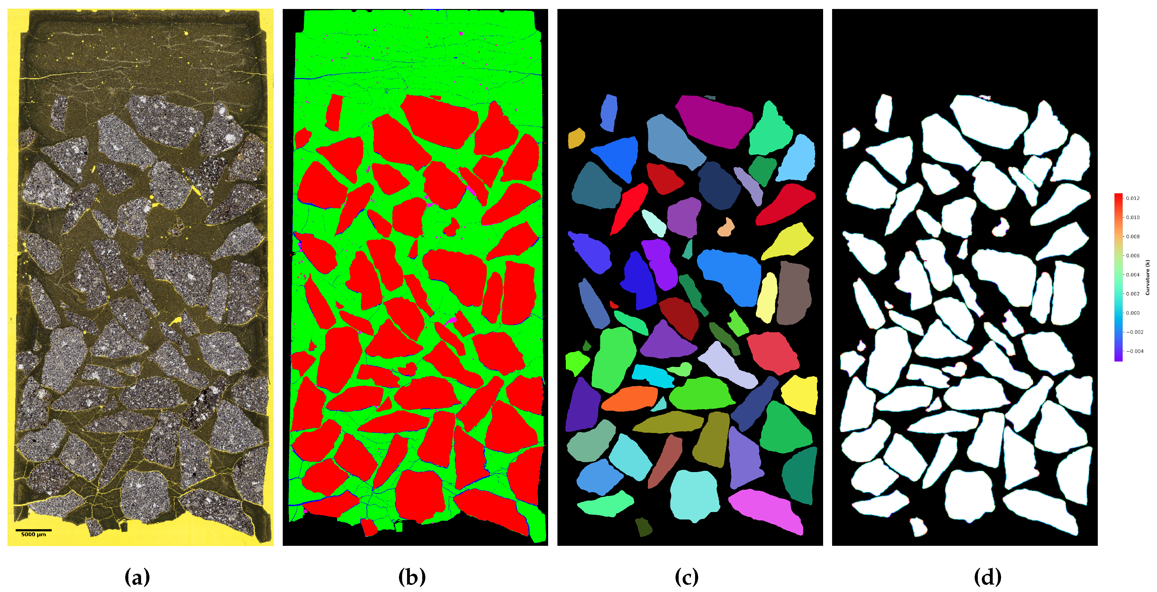
Aggregate boundaries (i.e., contours) are extracted in 2D and 3D, where the shape parameter Curvature (K) of boundaries for 2D and 3D shapes, proven to be effective in describing shape characteristics in cellular structures [81,84] and the cords lengths from the boundary points to the centroids. For air pores, centroids are estimated in 2D and 3D using peak local maxima of the normalised euclidean distance transform map with the value at the centre indicating the radius of each instance. Figure 10 and Figure 12(a) illustrate the process of curvature calculation for extracted shape instances in 2D and 3D respectively.
3.8. Feature Matching and Slice-to-Volume Registration
We study three different approaches of increasing processing time and complexity, namely feature matching of segmented LM and CT cross sections in 2D, 2D feature matching of segmented LM and 2D ROI patches extracted of 3D CT, and feature matching of segmented LM and CT in 3D.
3.8.1. Feature Matching of Segmented LM and CT Cross Sections in 2D
Shape feature matching using 2D Fourier Descriptors (FDs) is a technique that characterizes object boundaries by transforming spatial contour coordinates into the frequency domain. The shape’s boundary is represented as a sequence of complex numbers, , which serves as the input for a Discrete Fourier Transform (DFT). This transformation yields a set of complex coefficients, , known as Fourier Descriptors calculated using the formula:
where low-frequency components describe the general global shape and high-frequency components capture fine details like sharp corners, texture, noise. To ensure robust matching, these descriptors are normalized to be invariant to translation by setting , scale by normalizing by division of all coefficients by , rotation, and starting point by considering coefficient magnitudes . The final matching process involves comparing the Euclidean distance between the normalized feature vectors of different shapes using the Euclidean Distance Norm, allowing for efficient and noise-tolerant shape recognition.
For this approach, the central axis of the specimen is identified then sections at specific angle in the axial view are selected to extract point sets and contours from their respective segmentation masks. Figure 8 shows the slices extraction process on a CT scan of a cylindrical specimen at 3°dissection angles, whereas Figure 9 shows the steps of generating a 2D Fourier shape descriptor and the effect of lower order frequencies at varying numbers on the fidelity of the inverted shape in image domain.
Figure 8.
Slices extraction from a specimen along its longitudinal axis at 3 degrees. (a) Axial view of the CT specimen with the extracted cross-sections marked in red. (b) A layout of all target greyscale sections extracted. (c) Aggregate instance segmentation masks of (b).
Figure 8.
Slices extraction from a specimen along its longitudinal axis at 3 degrees. (a) Axial view of the CT specimen with the extracted cross-sections marked in red. (b) A layout of all target greyscale sections extracted. (c) Aggregate instance segmentation masks of (b).
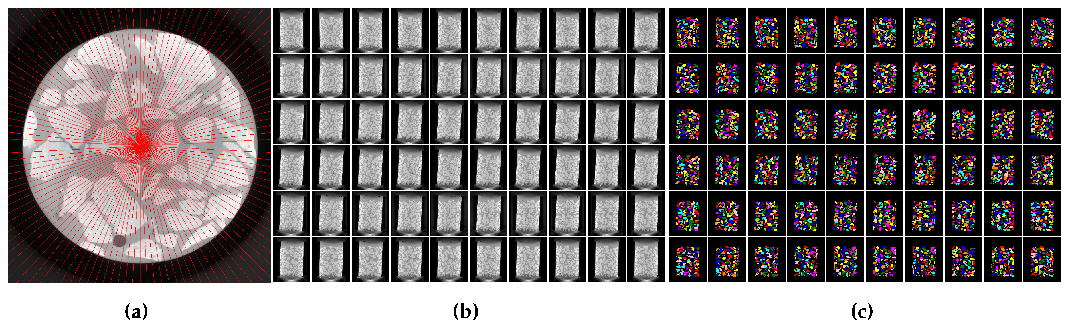
Figure 9.
Fourier Descriptors extraction for a slice of 3D CT Scan. (a) 3D view of the specimen. (b) Binary segmentation mask of aggregate labelled in red colour. (c) 3D Aggregate instances after processing. (d) 3D reconstructed models. (e) Inferred segmentation mask of the 2D slice. (f) Gravel instances of the 2D vertical slice. (g) Fourier shape descriptors for a sample particle marked in Sub-figure (f) at different harmonics n.
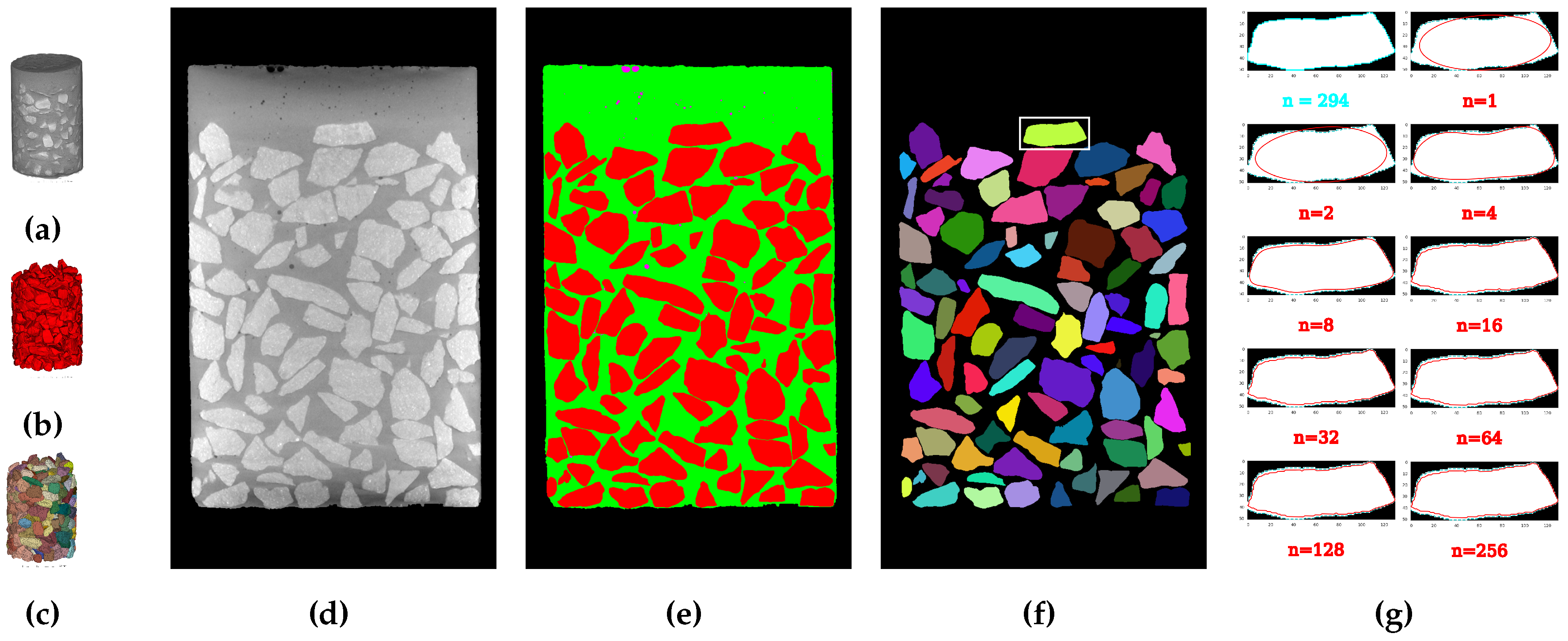
Figure 10.
Fourier Descriptors extraction for the Aggregate phase of a LM thin section. (a) The original RGB LM scan. (b) Its segmentation mask. (c) Aggregate instances assigned random colours. (d) Calculated curvatures of the contours to each gravel instance.
Figure 10.
Fourier Descriptors extraction for the Aggregate phase of a LM thin section. (a) The original RGB LM scan. (b) Its segmentation mask. (c) Aggregate instances assigned random colours. (d) Calculated curvatures of the contours to each gravel instance.
3.8.2. 2D Feature Matching of Segmented LM and 2D Patches of 3D CT
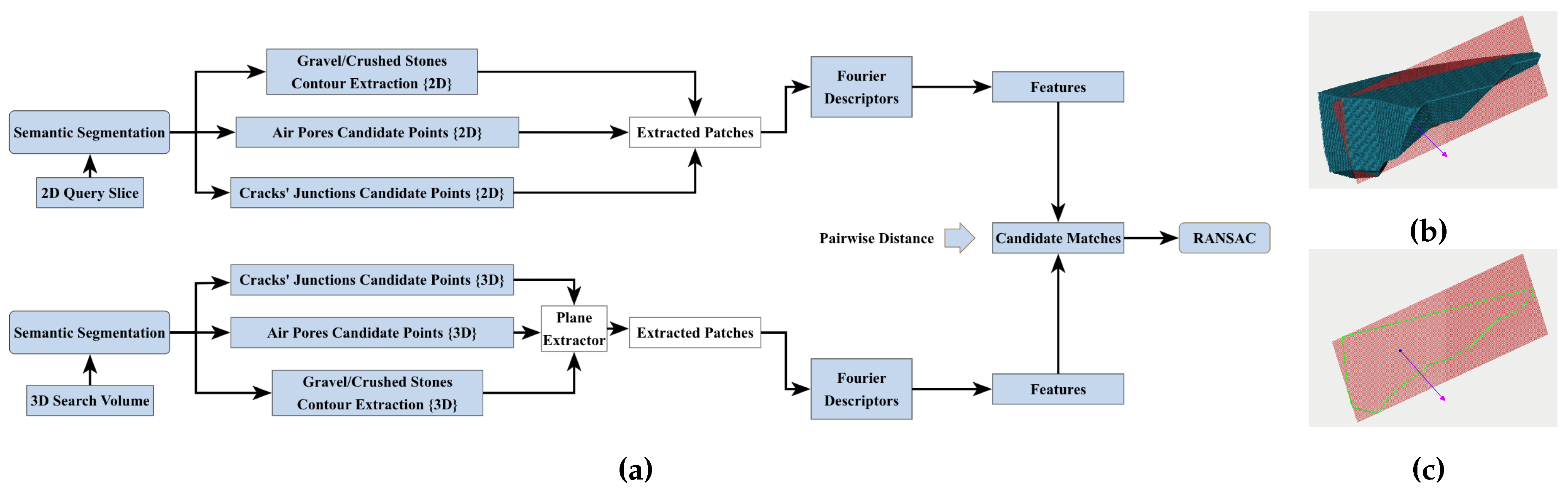
We adapt the workflow of Brandstätter et al. [67] summarised at Section 2.3 to achieve non-rigid registration by replacing the ReResNet module with the Fourier-based shape descriptor. Figure 11 shows a workflow diagram of the implemented pipeline and how a plane extractor dissects 3D shape instances into 2D.
Figure 11.
2D Feature Matching of Segmented LM and 2D ROI Patches of 3D CT. (a) A workflow diagram illustrating the modified approach to the feature matching registration. (b) A gravel instance with the dissector plane from one voxel of the voxelised downsampled shell orthogonal to radius of gyration with the shell’s voxel. (c) The extracted contour resulting from the boolean intersection of the plane with the voxel shell.
3.8.3. Feature Matching of Segmented LM and CT in 3D
We follow a shape normalisation method similar to the approach of [85,86] to register a 2D slice of the LM segmentation mask shapes projected into arbitrary 3D space to translation, rotation, reflection and scaling invariant shapes extracted from the 3D CT segmented stack. The registration is based on finding a best fit plane of matched features from the source and target. The formal theoretical background to the workflow is summarised below.
Canonical Normalisation of a 3D Shape
Let the original 3D shape be represented by a set of points , where each point . The goal is to find an affine transformation that maps P to a canonical representation for shape normalisation. This transformation is a composition of translation, rotation, reflection, and scaling operations. We apply translation invariance so that the shape is centred at the origin by subtracting its centroid c.
The translated point set is .
For rotation invariance, the orientation is standardised using Principal Component Analysis (PCA). We compute the covariance matrix C for the centred point set .
We then perform an eigen-decomposition of C to find its orthonormal eigenvectors . These eigenvectors form the rows of the rotation matrix R.
The rotated point set is defined as: .
For reflection invariance, ambiguity in the eigenvector directions is resolved by defining a reflection matrix F.
where are measures of asymmetry, such that the sum of the cubes of the coordinates: . The reflection-normalised point set is .
We apply scaling invariance of points to a standard size. The scaling factor s is computed as the root mean square distance of the points from the origin.
Consequently, the fully normalised point set is . The complete canonical transformation for any point p is:
Spherical Projection and Spatial Harmonic Analysis
The normalised 3D shape is used to generate rotation-invariant descriptors using the eigenbasis of the Laplace-Beltrami operator [87].
We then apply spherical coordinate conversion on the canonically normalised point set and project it onto a unit sphere. Each normalised point is projected onto the surface of the unit sphere by normalising its vector length, resulting in a set of points on the sphere .
To apply the discrete Laplace-Beltrami operator, the point set Q is structured into a triangular mesh , where are the vertices, E are the edges, and T are the triangles, typically constructed via spherical Delaunay triangulation.
We proceed to compute the Spatial Harmonic basis functions by solving the eigenvalue problem of the discrete Laplace-Beltrami operator (LBO) on the mesh M. We employ the Finite Element Method (FEM) discretization. This involves constructing the sparse mass matrix B and the stiffness matrix S. The entries of B are defined by the area of the mesh elements, and S is derived using the cotangent weight scheme. We solve the generalized symmetric definite eigenproblem:
where are the eigenvalues (spatial frequencies) and are the corresponding eigenvectors (spatial harmonic basis functions). These eigenvectors are B-orthonormal, satisfying .
The shape information (e.g., the radial distances of the original points ) is represented as a scalar function vector defined on the vertices V. This function is decomposed into the spatial harmonic basis by projecting f onto the eigenvectors using the B-inner product:
The resulting coefficients serve as the rotation-, translation-, reflection- and scaling-invariant shape descriptors vector for the local patch. Figure 12(a) illustrates the normalisation and spatial harmonics analysis on 4 gravel specimens selected from our case study, whereas Figure 12(b) shows the 40 lowest order basis functions (BF) from the spherical harmonics analysis on the normalised first shape instance.
Feature Matching in 3D Euclidean Space
Let there be a source shape S and a target shape T. Both are brought into their canonical forms, and . Local SPHARA descriptors are computed for keypoints on both shapes. Let be the descriptor vector of coefficients for keypoint and be the descriptor vector for keypoint . A match between keypoint i and keypoint j is established if the Euclidean distance between their spectral coefficient vectors is below a certain threshold .
This process yields a set of n matched point pairs . It is important to note that while the descriptors are calculated using the intermediate spectral representation on the mesh, the matching process links the original keypoints and . For the subsequent plane fitting, we use the set of these matched keypoints from the source shape, , which are already in 3D Euclidean coordinates.
Plane Estimation Using PCA
A 2D plane is fitted to the set of matched points in the normalised space using Principal Component Analysis (PCA). We calculate the centroid by computing the geometric centre of the matched points.
Then we construct the covariance matrix for the set .
We apply Eigen-decomposition to find the eigenvalues and corresponding eigenvectors of .
We define the best-fit plane for the matched points. The eigenvector associated with the smallest eigenvalue, , corresponds to the direction of least variance and is therefore the normal vector to the best-fit plane. The plane in the normalised space is defined by its normal vector and the point that lies on it. The plane equation is:
Figure 13 visually illustrates the process of feature matching and the plane fitting for source and target points on one of our case studies.
Inverse Transformation of the Fitted Plane
The plane is transformed back into the original coordinate system of the source shape S. This requires applying the inverse of the canonical transformation, . The forward transformation is , where the linear part is and the translation is . The inverse transformation acts on a point as:
Substituting the components of A, and noting that for orthogonal matrices and , the inverse linear part becomes . Thus:
A plane is defined by a point and a normal vector, which transform differently.
The point on the plane is transformed back to the original space:
A normal vector n transforms via the inverse transpose of the point transformation matrix. Since the points transform by , the normals transform by .
The final plane in the original 3D space is defined by the point and the normal vector . Its equation is:
Figure 12.
Canonical normalisation and Spatial Fourier Analysis of a Shape Descriptor via Discrete LBO. (a) Examples of 4 aggregate instances after canonical normalisation, calculating curvatures and conversion into frequency domain, inverting the lowest 256 harmonics into normalised image space. (b) The subplots of the Basis Functions (BF) 0-39 represent the lowest 40 frequencies describing the shape of the first gravel shape instance in the first row of sub-figure (a).
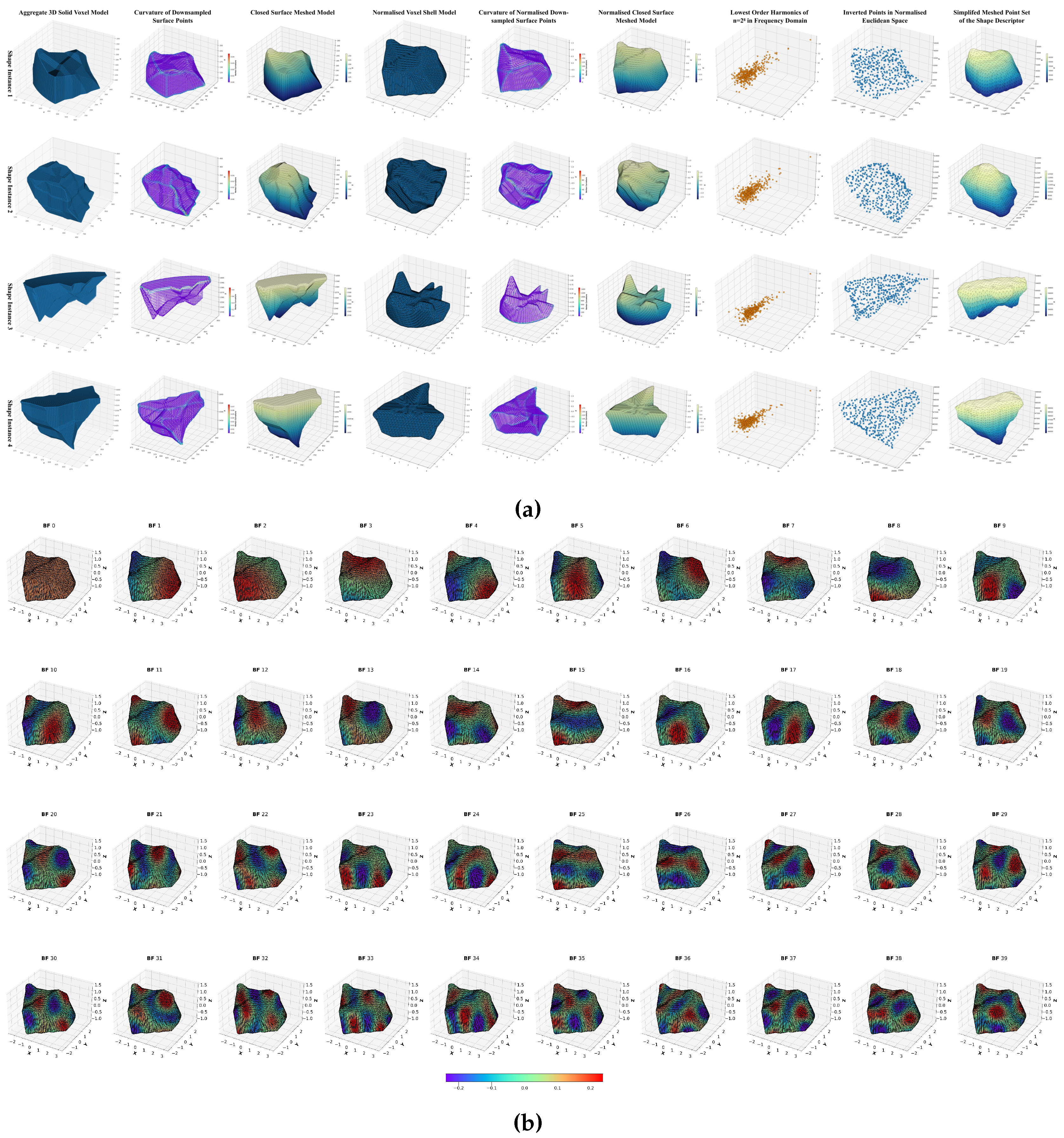
Figure 13.
Feature Matching and finding the best fit plane for source and target points using PCA. (a) Two dimensional projection of UMAP embeddings of the features space with the target overlapping features marked in black. (b) Best fit plane of canonically normalised matched point sets in Euclidean space.
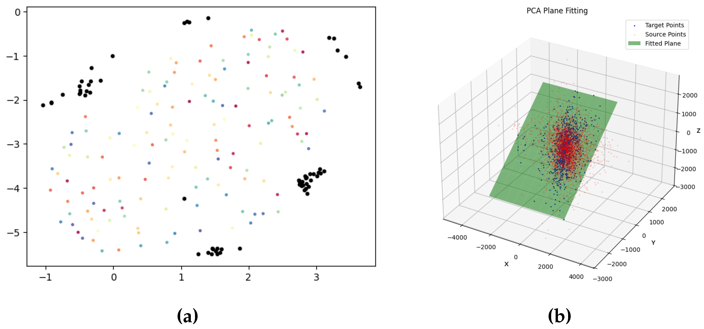
Figure 14.
Effect of the truncated lower order harmonics number n describing a 3D shape instance 3 in Figure 12(a) on its triangulated surface fidelity.
Figure 14.
Effect of the truncated lower order harmonics number n describing a 3D shape instance 3 in Figure 12(a) on its triangulated surface fidelity.
4. Experimental Setup
4.1. Synthetic Data Generation
We synthetically generate 3D annotated models to 30 cylindrical specimens containing the 5 phases, namely background, cracks, air pores, aggregate, and cement matrix as ground truths for testing our framework. The synthetic dataset eliminates the errors resulting from false positives and negatives from the segmentation predictions segmenting the LM thin section and the CT concrete specimens and potential mismatching due to minimal loss of some edge pieces during the petrographic sections preparation.
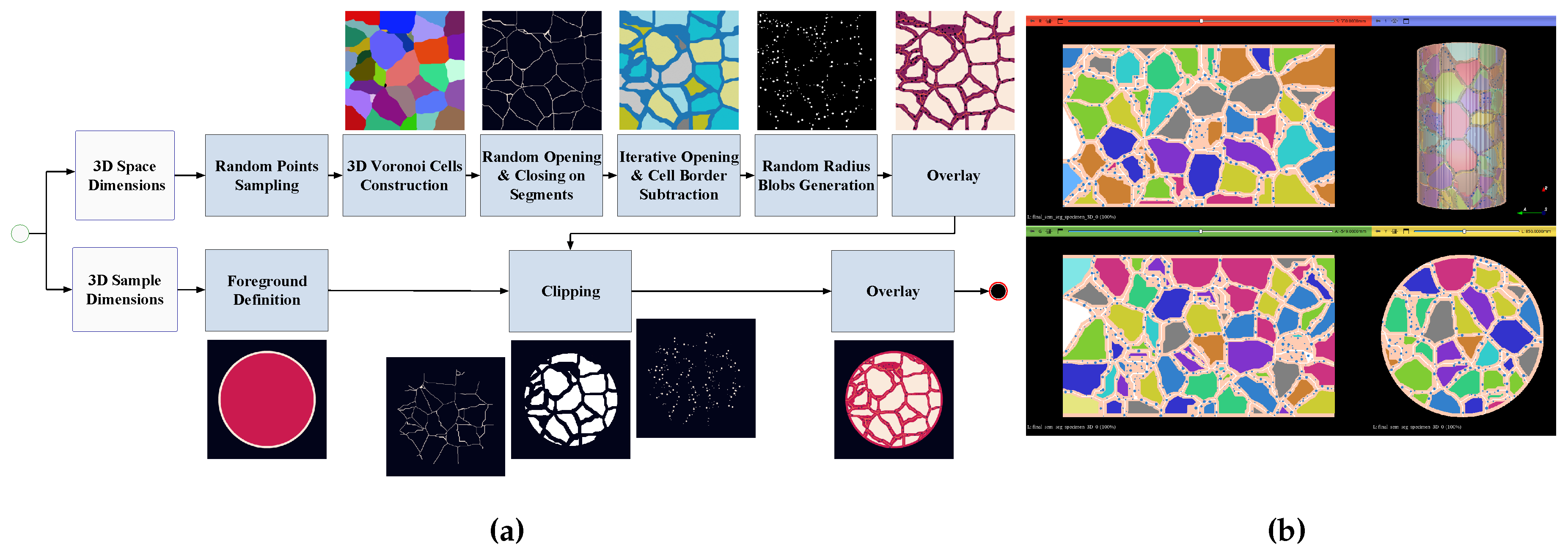
First, a 3D space perimeter is defined as well as the dimensions of the specimen. Second, from the sampled points we generate 3D Voronoi geometries filling the entire defined space. Third, the Voronoi edges are randomly opened and closed to generate cracks within a predefined range. Fourth, to model the aggregates, we iteratively apply voxel opening to thicken the edges of the space occupying the hydrated cement matrix, then apply logical subtraction of the edges to model aggregate. Fifth, the inner result is smoothed out using 3D B-Spline construction to simulate the gravel geometry for half the dataset and for the second half we use the sharp edged geometries generated to simulate crushed stone shapes. Sixth, air pores are added within the hydrated cement matrix regions by generating randomly sampled 3D blobs with a specified variable radius range. Finally all synthetic phases are laid over on top of each other and the background is subtracted from the space based on the defined specimen dimensions. Figure 15 demonstrates the developed pipeline for generating the synthetic specimens visually.
Figure 15.
Synthetic- data labels Dataset Generation. (a) Workflow for generating synthetic- data labels through Voronoi cell tessellated structures sampled from random points. (b) Example of synthetically generated specimen output overviewed in 3D Slicer.
Figure 15.
Synthetic- data labels Dataset Generation. (a) Workflow for generating synthetic- data labels through Voronoi cell tessellated structures sampled from random points. (b) Example of synthetically generated specimen output overviewed in 3D Slicer.
4.2. Optimal Parameters’ Selection
To determine the optimal configuration of points and features for the slice-to-volume registration, we study the different point-sets extracted from the 3 main classes of interest in the inferred segmentation of our 2D and 3D datasets: (1) Junction nodes of cracks , (2) Outer boundaries (i.e., contours) of aggregate instances , and (3) Centroids of air pores , as well as their combinations including (4) , (5) , (6) , (7) .
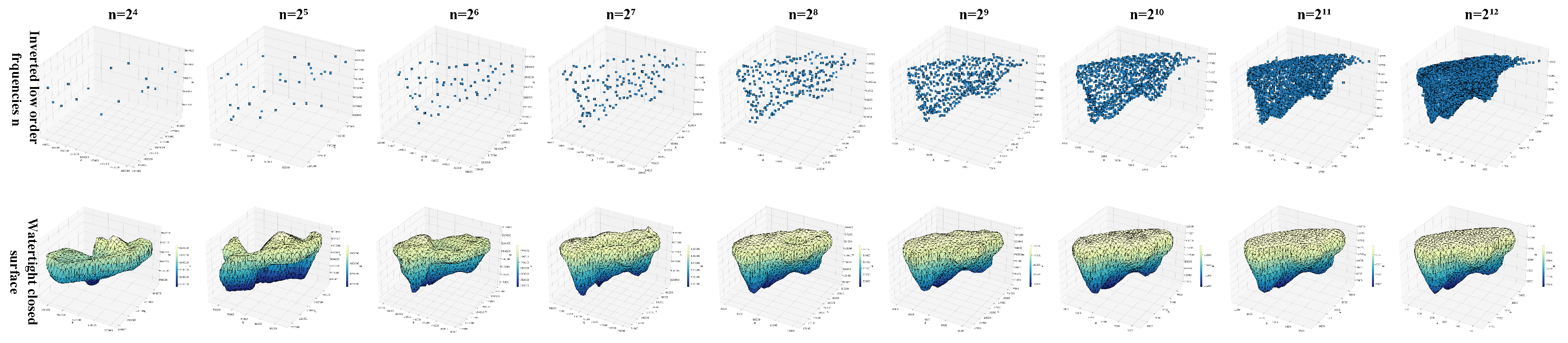
From the segmented instances of the main 3 classes of interest we generate the Fourier Descriptors to the canonically normalised contour point sets projected on a unit sphere in frequency domain and extract the optimal number of the lowest order frequencies to their basis functions that contain the describe the shape without losing too much fidelity measured by the Hausdorff distance and computational complexity estimated by processing time. The optimal number of frequencies was found to be harmonics. Figure 14 illustrates the effect of frequency order on the shape’s fidelity of a gravel instance.
4.2.1. Feature Analysis via Hierarchical Clustering
We investigate the shape features at the vertices of interest for relevance to the nearest neighbour search for aggregate shape point sets: Omnivariance, Eigentropy, Anisotropy, Planarity, Linearity, Surface Variation, Sphericity, Verticality, Curvature. Given the high dimensionality of the registration data that could lead to multicollinearity and higher correlation between target variables, we apply hierarchical clustering to identify relevant hierarchies in the feature space and use agglomerative nesting to calculate the correlation factors for the the features and and hierarchically sort them in a dendrogram for feature analysis. To limit the large memory requirement and processing time needed for the registration, we select the most relevant feature output, namely curvature.
5. Results
With optimal parameters selection, we iterated a set of 75 registration experiments on randomly extracted slices from the synthetic dataset and measured the relative root mean square error (RRMSE) for segmented labels between transformed source and target planes. The first framework in Section 3.8.1 performed the fastest but poorly with only 56.68% success rate and minimum scored RRMSE of 43.29%, when it converged to a solution. Experiments to clip the search space to a smaller interval improved the success rate slightly but did not result in a more accurate transformation. The second framework in Section 3.8.2 performed on average 22% slower in processing time than the first with a success rate of 69.88% of converging to a solution and scored a lower RRMSE with a minimum of 31.94%. The third framework in Section 3.8.3 performed the slowest with processing time occasionally exceeding 24 hours on a device with 16 cores Intel Xeon(R) W-11955M CPU, Nvidia RTX A5000 Mobile Graphics card and 128 GB memory space. The success rate of registration attempts was 89.75% and in almost 45% of failed iterations, it managed to converge to a solution on a second round with a different random seed with the lowest scored RRMSE of 5.21%. As only the third method provided an accurate and visually acceptable registration, we focus the scope of discussion about deployment on our case study and output results to it.
Figure 16.
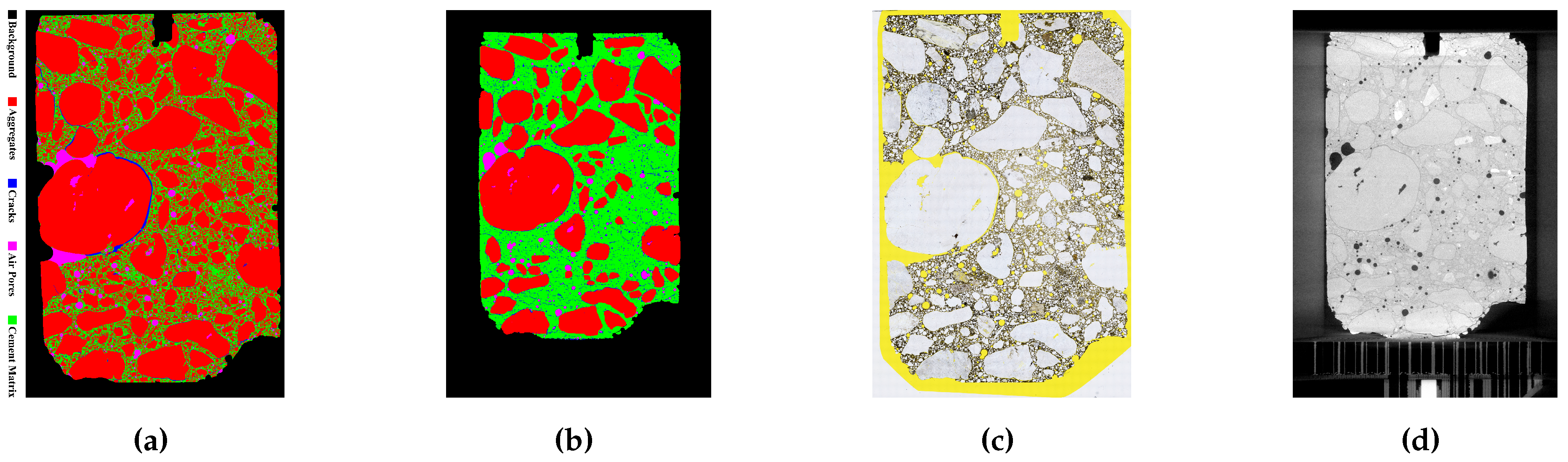
Result of case study source and matched best fit target of LM slice to CT volume registration. (a) Source LM segmentation mask. (b) Target CT segmentation mask. (c) Source LM petrographic scan. (d) Target CT slice.
Figure 16.
Result of case study source and matched best fit target of LM slice to CT volume registration. (a) Source LM segmentation mask. (b) Target CT segmentation mask. (c) Source LM petrographic scan. (d) Target CT slice.
For an objectively fair comparison of segmented phases between the registered LM and CT slices we detect a bounding box for the foreground in the CT slice and rectify the LM scan by computing the fundamental projective transformation 2D homography matrix H, for which holds through manual selection of seven corresponding points in both images and solving the linear homogeneous equation system using SVD, after conditioning the corresponding points through translation to the centroid and scaling the mean distance to their centroid to stabilise the solution. The homographic rectification results are shown in to the source LM image and the target CT image are shown in Figure 17(a),(b) respectively.
Figure 17.
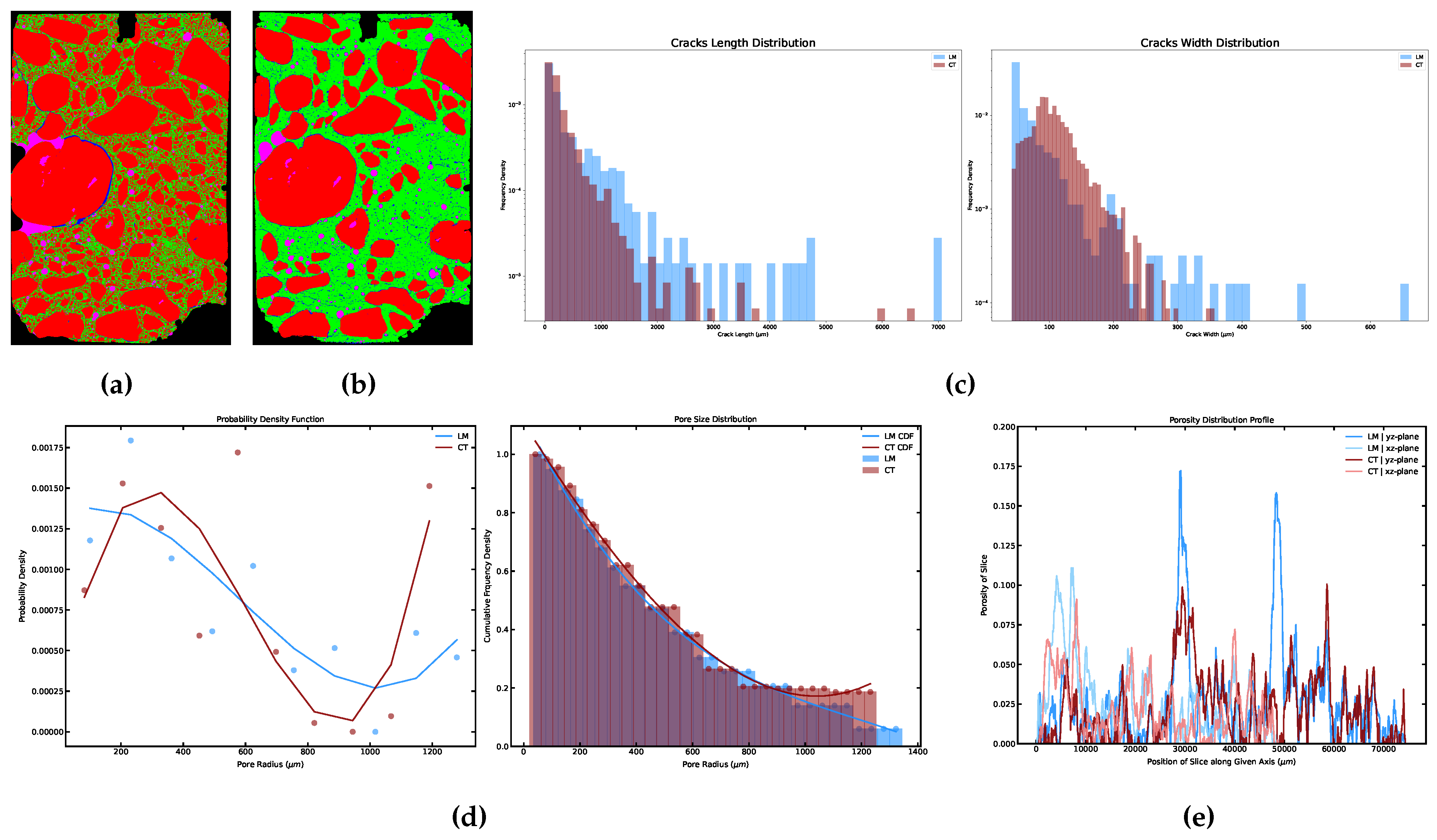
Results of 2D homographic rectification of LM slice and related segmentation mask to match CT and the the quantitative analysis of segmented cracks and air pores. (a) Source rectified LM segmentation mask. (b) Cropped CT Homography target segmentation mask. (c) Logarithmic scaled cracks lengths and widths distributions on the left and right respectively. (d) Calculated pores probability density function (PDF), cumulative density function (CDF) and the pores size distribution for LM and CT slices respectively. (e) Porosity profile along the principle axes for the LM and CT slices.
Figure 17.
Results of 2D homographic rectification of LM slice and related segmentation mask to match CT and the the quantitative analysis of segmented cracks and air pores. (a) Source rectified LM segmentation mask. (b) Cropped CT Homography target segmentation mask. (c) Logarithmic scaled cracks lengths and widths distributions on the left and right respectively. (d) Calculated pores probability density function (PDF), cumulative density function (CDF) and the pores size distribution for LM and CT slices respectively. (e) Porosity profile along the principle axes for the LM and CT slices.
5.1. Cracks and Pores Analysis
We analyse the cracks and air pores in the presented case study quantitatively after extracting the pixel size from the CT slice metadata of 20.8882 . For cracks, we extract the main cracks branches for a pixel graph of a simplified morphological skeleton of the cracks binary mask as elaborated in Section 3.7 and Figure 7 to calculate the lengths and mean width of every crack branch. A comparison of the length and width distribution of the segmented LM and CT cracks on a logarithmic scale is shown in Figure 17(c). Although both distributions show large correlation between crack lengths and mean widths across both modalities in the histograms, crack lengths are observed to diverge in the range above 800 with a relative difference in LM total cracks’ lengths to the CT calculated at 15.90%, whereas cracks’ mean widths in the range of 100 to 225 show a larger divergence with a relative difference in total cracks’ widths in CT to LM slice of around 20.07%.
PoreSpy library is used for the quantitative analysis of air pores in the LM and CT slices based on their relevant binary segmentation masks. The plots in Figure 17(d) show the pore size distributions in the LM and CT slices as well as the estimated probability density functions thereof. Figure 17(e) shows the porosity distribution profile along the principle axes. A higher degree of correlation is observed in their estimated pore size distribution than in cracks. The slight divergence in the radius size range above 1000 at the end of the estimated cumulative density curves could be attributed to the minor mislabelling errors occurring in the LM predicted segmentation mask due to the missing left edge pieces from the petrographic thin section already noticeable in Figure 16(c).
6. Discussion and Conclusion
We present three experimental workflows in this paper for solving the slice-to-volume registration problem. The framework is based mainly on the segmentation masks of their 2D slices and 3D stacks for the input and the transformation matrix output is estimated through finding a best fitted plane to matched shape descriptors generated from low order frequencies of the segmented instances. By applying canonical translation, rotation, scaling, and reflection-invariant normalisation to extracted shape instances from the 2/3D segmentation masks before conversion into frequency domain, we overcome the difference in pixel resolution and consequent scaling of input modalities and the inherent rigidity of similar registration methods to orthogonally aligned 3D planes caused by inevitable skewness from the axial plane during the cutting of thin sections from the concrete samples.
6.1. Limitations
The main observed limitation to our research is the long processing time needed for registration and instability of the third framework we deployed on the presented case study to succeed in converging into an optimal solution and delivering a stable transformation matrix output. Further study on stabilisation and conditioning mechanisms is needed for feature matching by limiting the searched feature space, point sets required or optimisation measures or the underlying shape descriptors used.
A the prerequisite to our presented registration method is the availability accurate segmentation masks as an input. Instance segmentation or semantic segmentation followed by instance extraction from concrete phases are another layer of technical challenges in itself considering the variables needed to acquire, process and annotate CT and LM data to train a task specific deep neural network (DNN) to generalise through supervised learning to robustly predict similar input. Factors like using different scanning devices, scanning settings, or introducing a different type of concrete specimens with different aggregate types, recycled concrete aggregate (RCA), textures, densities or admixtures, etc., may require retraining task-specific DNNs if they have not been included in the training dataset.
6.2. Future Work
Possible future work to consider is the application of our proposed framework onto bimodal semantic segmentation through data fusion for training neural network architectures to robustly segment cracks and better segment concrete phases in CT scans, like cement matrix and aggregate, especially when they possess similar density. Additionally, a reliable slice-to volume registration process for LM and CT scanning modalities paves the way for (a) automatically measuring the water uptake through the estimation of cementitious sorptivity via extracted data points from the inferred segmentation as proposed by [88], (b) Integrating state of the art 3D Discrete Fracture Network (DFN) Modelling approaches [89] for sampling the distributions of size, shape, orientation and other intrinsic properties to create plane network representation of cracks and air pores, compute mesh representations thereof [90,91,92,93,94,95], define boundary conditions (e.g., flow, transport, variable aperture, etc.) based on available CIF/CDF testing parameters and quantified segmentation estimations utilising state of the art open source software, like dfnWorks [96], pySimFrac [97], etc., and (c) modelling the Frost Resistance by approximation of the Loss Landscape surface of the trained model into a simpler function equation using regression fitting of polynomial and validating the quality of prediction through untrained sampled data points.
Author Contributions
Conceptualization, M.S.H.A.; methodology, M.S.H.A.; software, M.S.H.A; validation, M.S.H.A.; formal analysis, M.S.H.A.; investigation, M.S.H.A.; resources, M.S.H.A.; data curation, M.C.H, D.E.; writing—original draft preparation, M.S.H.A; writing—review and editing, M.S.H.A.; visualization, M.S.H.A; supervision, H.M.L. and A.O.; project administration, H.M.L. and A.O.; funding acquisition H.M.L. and A.O. All authors have read and agreed to the published version of the manuscript.
Funding
This research is funded by the Deutsche Forschungsgemeinschaft (DFG, German Research Foundation) - Project number 432767097. The APC is funded by the Open-Access Fund.
Data Availability Statement
Source code is available on GitHub. Synthetic-, , LM-Rissanalyse Datasets are available on Zenodo through the following Link.
Conflicts of Interest
The authors declare no conflicts of interest.
Abbreviations
The following abbreviations are used in this manuscript:
| CT | Micro Computed Tomography |
| LM | Light Microscopy |
| FT | Freezing and Thawing |
| DRI | Damage Rating Index method |
| ASR | Alkali-Silica Reaction |
| ISR | Internal Swelling Reaction |
| CDF | Capillary De-icing Freeze-thaw Test |
| CIF | Capillary Suction, Internal Damage and Freeze-thaw |
| DIC | Digital Image Correlation |
| FDCT | Fast Discrete Curvelet Transform |
| GLCM | Grey Level Co-occurrence Matrix |
| ANN | Artificial Neural Network |
| FFT | Fast Fourier Transform |
| FHT | Fast Haar Transform |
| LoG | Laplacian of Gaussian |
| CNN | Convolutional Neural Network |
| RBM | Restricted Boltzmann Machine |
| R-CNN | Region Convolutional Neural Network |
| RPN | Region Proposal Network |
| TuFF | Tubularity Flow Field |
| DTM | Distance Transform Method |
| STEGO | Self-supervised Transformer with Energy-based Graph Optimization |
| EAGLE | Eigen Aggregation Learning |
| ReResNet | rotation equivariant ResNet |
| RANSAC | Random Consensus |
| InShaDe | Invariant Shape Descriptors |
| FFF | Fused Filament Fabrication |
| PLA | Polylactic Acid |
| LMS | Least Mean Square |
| CLAHE | Contrast Limited Adaptive Histogram Equalisation |
| UMAP | Uniform Manifold Approximation and Projection |
| mIoU | mean Intersection over Union |
| SCUNet | Swin-Conv-UNet |
| CVAT | Computer Vision Annotation Tool |
| SAM | Segment Anything Model |
| TEASAR | tree-structure extraction algorithm delivering skeletons |
| that are accurate and robust | |
| EDT | Euclidean distance transform |
| CSR | Compressed Sparse Row |
| FD | Fourier Descriptor |
| DFT | Discrete Fourier Transform |
| LBO | Laplace-Beltrami Operator |
| FEM | Finite Element Method |
| PCA | Principal Component Analysis |
| SVD | Singular value decomposition |
| BF | Basis Function |
| RRMSE | Relative root mean square error |
| DNN | Deep Neural Network |
| RCA | Recycled Concrete Aggregate |
| DFN | Discrete Fracture Network |
References
- Li, H.; Wu, X.; Nie, Q.; Yu, J.; Zhang, L.; Wang, Q.; Gao, Q. Lifetime prediction of damaged or cracked concrete structures: A review. Structures 2025, 71, 108095. [CrossRef]
- Arasteh-Khoshbin, O.; Seyedpour, S.M.; Brodbeck, M.; Lambers, L.; Ricken, T. On effects of freezing and thawing cycles of concrete containing nano-Formula: see text: experimental study of material properties and crack simulation. Scientific reports 2023, 13, 22278. [CrossRef]
- 5 - Concrete. In Building Materials in Civil Engineering; Haimei Zhang., Ed.; Woodhead Publishing Series in Civil and Structural Engineering, Woodhead Publishing, 2011; pp. 81–423. [CrossRef]
- Abell, A.B.; Willis, K.L.; Lange, D.A. Mercury Intrusion Porosimetry and Image Analysis of Cement-Based Materials. Journal of colloid and interface science 1999, 211, 39–44. [CrossRef]
- ACI Committee 224. 224R-01: Control of Cracking in Concrete Structures (Reapproved 2008). Technical Documents.
- Bisschop, J.; van Mier, J. How to study drying shrinkage microcracking in cement-based materials using optical and scanning electron microscopy? Cement and Concrete Research 2002, 32, 279–287. [CrossRef]
- Patzelt, M.; Erfurt, D.; Ludwig, H.M. Quantification of cracks in concrete thin sections considering current methods of image analysis. Journal of microscopy 2022, 286, 154–159. [CrossRef]
- Patzelt, M.; Erfurt, D.; Hadlich, C.; Vogt, F.; Ludwig, H.M.; Osburg, A. Verknüpfung & Automatisierung computergestützter Methoden zur quantitativen Rissanalyse von Beton. ce/papers 2023, 6, 1086–1090. [CrossRef]
- Grattan-Bellew, P.E.; Danay, A. Comparison of laboratory and field evaluation of alkali- silica reaction in large dams. 1992, International Conference on Concrete Alkali-aggregate Reactions in Hydroelectric Plants and Dams: 28 September 1992, Frederiction, New Brunswick, Canada, pp. 1–25.
- Dunbar, P.A.; Grattan-Bellew, P.E. Results of damage rating evaluation of condition of concrete from a number of structures affected by AAR. Natural Resources Canada, 1995, CANMET/ACI International Workshop on Alkali-Aggregate Reactions in Concrete, October 1 to 4, 1995, Dartmouth, Nova Scotia, Canada, pp. 257–265.
- Zahedi, A.; Trottier, C.; Sanchez, L.F.; Noël, M. Microscopic assessment of ASR-affected concrete under confinement conditions. Cement and Concrete Research 2021, 145, 106456. [CrossRef]
- Villeneuve, V.; Fournier, B.; Duchesne, J. Determination of the damage in concrete affected by ASR–the damage rating index (DRI). In Proceedings of the 14th International Conference on Alkali-Aggregate Reaction (ICAAR). Austin, Texas (USA), 2012.
- Sanchez, L.; Fournier, B.; Jolin, M.; Mitchell, D.; Bastien, J. Overall assessment of Alkali-Aggregate Reaction (AAR) in concretes presenting different strengths and incorporating a wide range of reactive aggregate types and natures. Cement and Concrete Research 2017, 93, 17–31. [CrossRef]
- Martin, R.P.; Sanchez, L.; Fournier, B.; Toutlemonde, F.c. Diagnosis of AAR and DEF: Comparison of residual expansion, stiffness damage test and damage rating index. In Proceedings of the ICAAR 2016 - 15th international conference on alkali aggregate reaction, Sao Paulo, France, 2016; p. 10p.
- Sanchez, L.; Drimalas, T.; Fournier, B. Assessing condition of concrete affected by internal swelling reactions (ISR) through the Damage Rating Index (DRI). Cement 2020, 1-2, 100001. [CrossRef]
- DIN-Fachbericht CEN/TR 15177:2006-06, Prüfung des Frost-Tauwiderstandes von Beton_- Innere Gefügestörung; Deutsche Fassung CEN/TR_15177:2006. [CrossRef]
- Setzer, M.J.; Fagerlund, G.; Janssen, D.J. CDF test — Test method for the freeze-thaw resistance of concrete-tests with sodium chloride solution (CDF). Materials and Structures 1996, 29, 523–528. [CrossRef]
- Setzer, M.J.; Heine, P.; Kasparek, S.; Palecki, S.; Auberg, R.; Feldrappe, V.; Siebel, E. Test methods of frost resistance of concrete: CIF-Test: Capillary suction, internal damage and freeze thaw test—Reference method and alternative methods A and B. Materials and Structures 2004, 37, 743–753. [CrossRef]
- Gong, F.; Zhi, D.; Jia, J.; Wang, Z.; Ning, Y.; Zhang, B.; Ueda, T. Data-Based Statistical Analysis of Laboratory Experiments on Concrete Frost Damage and Its Implications on Service Life Prediction. Materials (Basel, Switzerland) 2022, 15. [CrossRef]
- Rath, S.; Ji, X.; Takahashi, Y.; Tanaka, S.; Sakai, Y. Evaluating concrete quality under freeze–thaw damage using the drilling powder method. Journal of Sustainable Cement-Based Materials 2025, 14, 253–264. [CrossRef]
- Liu, Z.; Hansen, W. Freeze–thaw durability of high strength concrete under deicer salt exposure. Construction and Building Materials 2016, 102, 478–485. [CrossRef]
- Auberg, R. Application of CIF-Test in practise for reliable evaluation of frost resistance of concrete. In Proceedings of the International RILEM Workshop on Frost Resistance of Concrete, 2002, pp. 255–267.
- Hanjari, K.Z.; Utgenannt, P.; Lundgren, K. Experimental study of the material and bond properties of frost-damaged concrete. Cement and Concrete Research 2011, 41, 244–254. [CrossRef]
- Ebrahimi, K.; Daiezadeh, M.J.; Zakertabrizi, M.; Zahmatkesh, F.; Habibnejad Korayem, A. A review of the impact of micro- and nanoparticles on freeze-thaw durability of hardened concrete: Mechanism perspective. Construction and Building Materials 2018, 186, 1105–1113. [CrossRef]
- Spörel, F. Freeze-Thaw-Attack on concrete structures -laboratory tests, monitoring, practical experience. In Proceedings of the International RILEM Conference on Materials, Systems and Structures in Civil Engineering Conference segment on Frost Action in Concrete 22-23 August 2016, Technical University of Denmark, Lyngby, Denmark; Tange Hasholt, M.; Fridh, K.; Hooton, R.D., Eds., 2016, p. 151.
- Barisin, T.; Jung, C.; Nowacka, A.; Redenbach, C.; Schladitz, K. Cracks in Concrete; Vol. 227, pp. 263–280. [CrossRef]
- Zakeri, H.; Nejad, F.M.; Fahimifar, A. Image Based Techniques for Crack Detection, Classification and Quantification in Asphalt Pavement: A Review. Archives of Computational Methods in Engineering 2017, 24, 935–977. [CrossRef]
- Mohan, A.; Poobal, S. Crack detection using image processing: A critical review and analysis. Alexandria Engineering Journal 2018, 57, 787–798. [CrossRef]
- Nazaryan, N.; Campana, C.; Moslehpour, S.; Shetty, D. Application of a He3Ne infrared laser source for detection of geometrical dimensions of cracks and scratches on finished surfaces of metals. Optics and Lasers in Engineering 2013, 51, 1360–1367. [CrossRef]
- Anwar, S.A.; Abdullah, M.Z. Micro-crack detection of multicrystalline solar cells featuring an improved anisotropic diffusion filter and image segmentation technique. EURASIP Journal on Image and Video Processing 2014, 2014. [CrossRef]
- Heideklang, R.; Shokouhi, P. Multi-sensor image fusion at signal level for improved near-surface crack detection. NDT & E International 2015, 71, 16–22. [CrossRef]
- Chen, X.; Michaels, J.E.; Lee, S.J.; Michaels, T.E. Load-differential imaging for detection and localization of fatigue cracks using Lamb waves. NDT & E International 2012, 51, 142–149. [CrossRef]
- Alam, S.Y.; Loukili, A.; Grondin, F.; Rozière, E. Use of the digital image correlation and acoustic emission technique to study the effect of structural size on cracking of reinforced concrete. Engineering Fracture Mechanics 2015, 143, 17–31. [CrossRef]
- Brooks, W.S.M.; Lamb, D.A.; Irvine, S.J.C. IR Reflectance Imaging for Crystalline Si Solar Cell Crack Detection. IEEE Journal of Photovoltaics 2015, 5, 1271–1275. [CrossRef]
- Hamrat, M.; Boulekbache, B.; Chemrouk, M.; Amziane, S. Flexural cracking behavior of normal strength, high strength and high strength fiber concrete beams, using Digital Image Correlation technique. Construction and Building Materials 2016, 106, 678–692. [CrossRef]
- Iliopoulos, S.; Aggelis, D.G.; Pyl, L.; Vantomme, J.; van Marcke, P.; Coppens, E.; Areias, L. Detection and evaluation of cracks in the concrete buffer of the Belgian Nuclear Waste container using combined NDT techniques. Construction and Building Materials 2015, 78, 369–378. [CrossRef]
- Gunkel, C.; Stepper, A.; Müller, A.C.; Müller, C.H. Micro crack detection with Dijkstra’s shortest path algorithm. Machine Vision and Applications 2012, 23, 589–601. [CrossRef]
- Glud, J.A.; Dulieu-Barton, J.M.; Thomsen, O.T.; Overgaard, L. Automated counting of off-axis tunnelling cracks using digital image processing. Composites Science and Technology 2016, 125, 80–89. [CrossRef]
- Li, X.; Jiang, H.; Yin, G. Detection of surface crack defects on ferrite magnetic tile. NDT & E International 2014, 62, 6–13. [CrossRef]
- Kabir, S. Imaging-based detection of AAR induced map-crack damage in concrete structure. NDT & E International 2010, 43, 461–469. [CrossRef]
- Abdel-Qader, I.; Abudayyeh, O.; Kelly, M.E. Analysis of Edge-Detection Techniques for Crack Identification in Bridges. Journal of Computing in Civil Engineering 2003, 17, 255–263. [CrossRef]
- Ni, F.; Zhang, J.; Chen, Z. Pixel-level crack delineation in images with convolutional feature fusion. Structural Control and Health Monitoring 2019, 26, e2286. [CrossRef]
- LeCun, Y.; Bengio, Y.; Hinton, G. Deep learning. Nature 2015, 521, 436–444. [CrossRef]
- Dorafshan, S.; Thomas, R.J.; Maguire, M. Comparison of deep convolutional neural networks and edge detectors for image-based crack detection in concrete. Construction and Building Materials 2018, 186, 1031–1045. [CrossRef]
- Zhang, Y.; Sohn, K.; Villegas, R.; Pan, G.; Lee, H. Improving object detection with deep convolutional networks via Bayesian optimization and structured prediction; pp. 249–258. [CrossRef]
- Xu, Y.; Li, S.; Zhang, D.; Jin, Y.; Zhang, F.; Li, N.; Li, H. Identification framework for cracks on a steel structure surface by a restricted Boltzmann machines algorithm based on consumer-grade camera images. Structural Control and Health Monitoring 2018, 25, e2075. [CrossRef]
- Fan, R.; Bocus, M.J.; Zhu, Y.; Jiao, J.; Wang, L.; Ma, F.; Cheng, S.; Liu, M. Road Crack Detection Using Deep Convolutional Neural Network and Adaptive Thresholding; pp. 474–479. [CrossRef]
- Liu, Y.; Yao, J.; Lu, X.; Xie, R.; Li, L. DeepCrack: A deep hierarchical feature learning architecture for crack segmentation. Neurocomputing 2019, 338, 139–153. [CrossRef]
- Zou, Q.; Zhang, Z.; Li, Q.; Qi, X.; Wang, Q.; Wang, S. DeepCrack: Learning Hierarchical Convolutional Features for Crack Detection. IEEE transactions on image processing : a publication of the IEEE Signal Processing Society 2018. [CrossRef]
- Benz, C.; Debus, P.; Ha, H.K.; Rodehorst, V. Crack Segmentation on UAS-based Imagery using Transfer Learning; pp. 1–6. [CrossRef]
- Iglovikov, V.; Shvets, A. TernausNet: U-Net with VGG11 Encoder Pre-Trained on ImageNet for Image Segmentation. ArXiv 2018, abs/1801.05746.
- Kang, D.; Benipal, S.S.; Gopal, D.L.; Cha, Y.J. Hybrid pixel-level concrete crack segmentation and quantification across complex backgrounds using deep learning. Automation in Construction 2020, 118, 103291. [CrossRef]
- Girshick, R. Fast R-CNN; pp. 1440–1448. [CrossRef]
- Mukherjee, S.; Condron, B.; Acton, S.T. Tubularity flow field–a technique for automatic neuron segmentation. IEEE transactions on image processing : a publication of the IEEE Signal Processing Society 2015, 24, 374–389. [CrossRef]
- Barisin, T.; Jung, C.; Müsebeck, F.; Redenbach, C.; Schladitz, K. Methods for segmenting cracks in 3d images of concrete: A comparison based on semi-synthetic images. Pattern Recognition 2022, 129, 108747. [CrossRef]
- Shi, Y.; Cui, L.; Qi, Z.; Meng, F.; Chen, Z. Automatic Road Crack Detection Using Random Structured Forests. IEEE Transactions on Intelligent Transportation Systems 2016, 17, 3434–3445. [CrossRef]
- Chun, P.j.; Izumi, S.; Yamane, T. Automatic detection method of cracks from concrete surface imagery using two–step light gradient boosting machine. Computer-Aided Civil and Infrastructure Engineering 2021, 36, 61–72. [CrossRef]
- Arganda-Carreras, I.; Kaynig, V.; Rueden, C.; Eliceiri, K.W.; Schindelin, J.; Cardona, A.; Sebastian Seung, H. Trainable Weka Segmentation: a machine learning tool for microscopy pixel classification. Bioinformatics (Oxford, England) 2017, 33, 2424–2426. [CrossRef]
- Sadrnia, A.; Alabassy, M.S.H.; Osburg, A. Unsupervised Semantic Segmentation of Cracks in Concrete Specimens. In 36th Forum Bauinformatik 2025; Willmann, A.; Kobbelt, L., Eds.; RWTH Aachen University: Aachen, 2025. [CrossRef]
- Hamilton, M.; Zhang, Z.; Hariharan, B.; Snavely, N.; Freeman, W.T. Unsupervised Semantic Segmentation by Distilling Feature Correspondences. [CrossRef]
- Kim, C.; Han, W.; Ju, D.; Hwang, S.J. EAGLE: Eigen Aggregation Learning for Object-Centric Unsupervised Semantic Segmentation. [CrossRef]
- Patzelt, M.; Hampe, M. µCT-scans of a selection of concrete samples made of cement and coarse aggregates without sand fraction. [CrossRef]
- Çiçek, Ö.; Abdulkadir, A.; Lienkamp, S.S.; Brox, T.; Ronneberger, O. 3D U-Net: Learning Dense Volumetric Segmentation from Sparse Annotation. [CrossRef]
- Ronneberger, O.; Fischer, P.; Brox, T. U-Net: Convolutional Networks for Biomedical Image Segmentation. [CrossRef]
- Dobrovolskij, D.; Persch, J.; Schladitz, K.; Steidl, G. STRUCTURE DETECTION WITH SECOND ORDER RIESZ TRANSFORMS. Image Analysis & Stereology 2019, 38, 107. [CrossRef]
- Çiçek, Ö.; Abdulkadir, A.; Lienkamp, S.S.; Brox, T.; Ronneberger, O. 3D U-Net: Learning Dense Volumetric Segmentation from Sparse Annotation. [CrossRef]
- Brandstätter, S.; Seeböck, P.; Fürböck, C.; Pochepnia, S.; Prosch, H.; Langs, G. Rigid Single-Slice-in-Volume Registration via Rotation-Equivariant 2D/3D Feature Matching. In Biomedical Image Registration; Modat, M.; Simpson, I.; Špiclin, Ž.; Bastiaansen, W.; Hering, A.; Mok, T.C.W., Eds.; Springer Nature Switzerland: Cham, 2024; Vol. 15249, Lecture Notes in Computer Science, pp. 280–294. [CrossRef]
- Al-Thelaya, K.; Agus, M.; Gilal, N.U.; Yang, Y.; Pintore, G.; Gobbetti, E.; Calí, C.; Magistretti, P.J.; Mifsud, W.; Schneider, J. InShaDe: Invariant Shape Descriptors for visual 2D and 3D cellular and nuclear shape analysis and classification. Computers & Graphics 2021, 98, 105–125. [CrossRef]
- Onajite, E. Understanding Sample Data. In Seismic Data Analysis Techniques in Hydrocarbon Exploration; Elsevier, 2014; pp. 105–115. [CrossRef]
- Fazekas, K., Ed. Proceedings of ECMCS- 2001, the 3 rd EURASIP Conference on Digital Signal Processing for Multimedia Communications and Services, 11 - 13 September 2001, Budapest, Hungary, Budapest, 2001. Scientific Assoc. of Infocommunications.
- Zuiderveld, K. Contrast limited adaptive histogram equalization. In Graphics gems IV; 1994; pp. 474–485.
- McInnes, L.; Healy, J.; Melville, J. UMAP: Uniform Manifold Approximation and Projection for Dimension Reduction. [CrossRef]
- Attias, H. A variational Bayesian framework for graphical models. In Proceedings of the Proceedings of the 13th International Conference on Neural Information Processing Systems, Cambridge, MA, USA, 1999; NIPS’99, pp. 209–215.
- Blei, D.M.; Jordan, M.I. Variational inference for Dirichlet process mixtures. Bayesian Analysis 2006, 1. [CrossRef]
- Russell, B.C.; Torralba, A.; Murphy, K.P.; Freeman, W.T. LabelMe: A Database and Web-Based Tool for Image Annotation. International Journal of Computer Vision 2008, 77, 157–173. [CrossRef]
- Ni, Z.L.; Bian, G.B.; Zhou, X.H.; Hou, Z.G.; Xie, X.L.; Wang, C.; Zhou, Y.J.; Li, R.Q.; Li, Z. RAUNet: Residual Attention U-Net for Semantic Segmentation of Cataract Surgical Instruments. [CrossRef]
- Zhang, K.; Li, Y.; Liang, J.; Cao, J.; Zhang, Y.; Tang, H.; Fan, D.P.; Timofte, R.; van Gool, L. Practical Blind Image Denoising via Swin-Conv-UNet and Data Synthesis. Machine Intelligence Research 2023, 20, 822–836. [CrossRef]
- CVAT.ai Corporation. Computer Vision Annotation Tool (CVAT), 2024. [CrossRef]
- Kirillov, A.; Mintun, E.; Ravi, N.; Mao, H.; Rolland, C.; Gustafson, L.; Xiao, T.; Whitehead, S.; Berg, A.C.; Lo, W.Y.; et al. Segment Anything. [CrossRef]
- Stringer, C.; Pachitariu, M. Cellpose3: one-click image restoration for improved cellular segmentation. Nature methods 2025, 22, 592–599. [CrossRef]
- William Silversmith.; J. Alexander Bae.; Peter H. Li.; A.M. Wilson. Kimimaro: Skeletonize Densely Labeled Images, 2021. [CrossRef]
- Sato, Y.; Westin, C.; Bhalerao, A.; Nakajima, S.; Shiraga, N.; Tamura, S.; Kikinis, R. Tissue classification based on 3D local intensity structures for volume rendering. IEEE Transactions on Visualization and Computer Graphics 2000, 6, 160–180. [CrossRef]
- Nunez-Iglesias, J.; Blanch, A.J.; Looker, O.; Dixon, M.W.; Tilley, L. A new Python library to analyse skeleton images confirms malaria parasite remodelling of the red blood cell membrane skeleton. PeerJ 2018, 6, e4312. [CrossRef]
- Driscoll, M.K.; McCann, C.; Kopace, R.; Homan, T.; Fourkas, J.T.; Parent, C.; Losert, W. Cell shape dynamics: from waves to migration. PLoS computational biology 2012, 8, e1002392. [CrossRef]
- Vranic, D.; Saupe, D. 3D Shape Descriptor Based on 3D Fourier Transform; pp. 271–274.
- Heczko, M.; Keim, D.; Saupe, D.; Vranić, D.V. Verfahren zur Ähnlichkeitssuche auf 3D-Objekten; pp. 384–401. [CrossRef]
- Graichen, U.; Eichardt, R.; Fiedler, P.; Strohmeier, D.; Zanow, F.; Haueisen, J. SPHARA–a generalized spatial Fourier analysis for multi-sensor systems with non-uniformly arranged sensors: application to EEG. PloS one 2015, 10, e0121741. [CrossRef]
- Kabir, H.; Wu, J.; Dahal, S.; Joo, T.; Garg, N. Automated estimation of cementitious sorptivity via computer vision. Nature communications 2024, 15, 9935. [CrossRef]
- Viswanathan, H.S.; Ajo-Franklin, J.; Birkholzer, J.T.; Carey, J.W.; Guglielmi, Y.; Hyman, J.D.; Karra, S.; Pyrak-Nolte, L.J.; Rajaram, H.; Srinivasan, G.; et al. From Fluid Flow to Coupled Processes in Fractured Rock: Recent Advances and New Frontiers. Reviews of Geophysics 2022, 60. [CrossRef]
- Hyman, J.D.; Smolarkiewicz, P.K.; Winter, C.L. Heterogeneities of flow in stochastically generated porous media. Physical review. E, Statistical, nonlinear, and soft matter physics 2012, 86, 056701. [CrossRef]
- Hyman, J.D.; Winter, C.L. Hyperbolic regions in flows through three-dimensional pore structures. Physical review. E, Statistical, nonlinear, and soft matter physics 2013, 88, 063014. [CrossRef]
- Hyman, J.D.; Winter, C.L. Hyperbolic regions in flows through three-dimensional pore structures. Physical review. E, Statistical, nonlinear, and soft matter physics 2013, 88, 063014. [CrossRef]
- Hyman, J.D.; Gable, C.W.; Painter, S.L.; Makedonska, N. Conforming Delaunay Triangulation of Stochastically Generated Three Dimensional Discrete Fracture Networks: A Feature Rejection Algorithm for Meshing Strategy. SIAM Journal on Scientific Computing 2014, 36, A1871–A1894. [CrossRef]
- Hyman, J.D.; Guadagnini, A.; Winter, C.L. Statistical scaling of geometric characteristics in stochastically generated pore microstructures. Computational Geosciences 2015, 19, 845–854. [CrossRef]
- Hyman, J.D.; Sweeney, M.R.; Frash, L.P.; Carey, J.W.; Viswanathan, H.S. Scale–Bridging in Three–Dimensional Fracture Networks: Characterizing the Effects of Variable Fracture Apertures on Network–Scale Flow Channelization. Geophysical Research Letters 2021, 48. [CrossRef]
- Hyman, J.D.; Karra, S.; Makedonska, N.; Gable, C.W.; Painter, S.L.; Viswanathan, H.S. dfnWorks: A discrete fracture network framework for modeling subsurface flow and transport. Computers & Geosciences 2015, 84, 10–19. [CrossRef]
- Guiltinan, E.; Santos, J.E.; Purswani, P.; Hyman, J.D. pySimFrac: A Python library for synthetic fracture generation and analysis. Computers & Geosciences 2024, 191, 105665. [CrossRef]
Figure 1.
Pipeline for Optimal beam hardening correction through image processing demonstrated on an exemplary original greyscale 2D slice image from the 3D CT stack.
Figure 1.
Pipeline for Optimal beam hardening correction through image processing demonstrated on an exemplary original greyscale 2D slice image from the 3D CT stack.
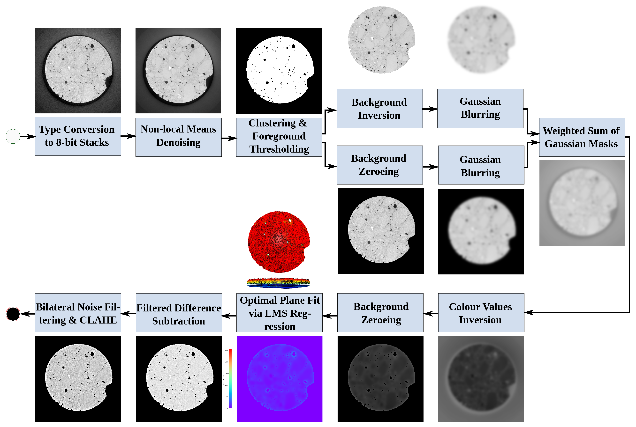
Figure 3.
Dataset preprocessing steps displayed on a patch and full scan sample of petrographic thin sections of the concrete specimens. (a) Coloured RGB microscopy scan. (b) Intermediate mask generated using UMAP feature embeddings and Bayesian Gaussian Mixture for enhanced clustering. (c) Final annotation mask generated semi-automatically by aggregating sub-clusters together and cleaning inaccuracies using automated annotation tool LabelMe.
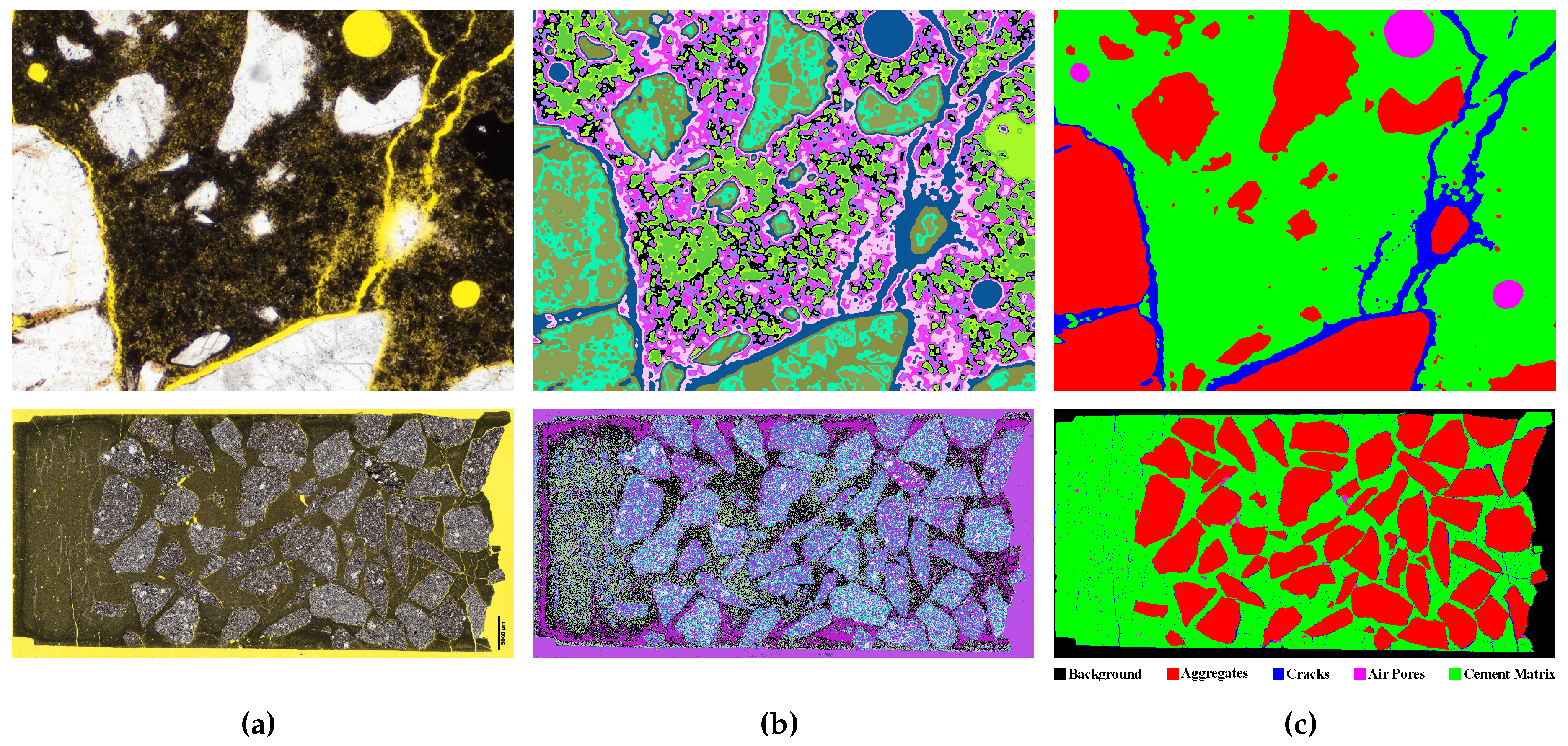
Figure 4.
Learning Curves of retrained Attention Residual UNet on the LM Dataset. (a) Accuracy Curves for training and validation sets. (b) Loss Curves for training and validation sets. (c) Inference results of the trained DNN on some validation samples.
Figure 4.
Learning Curves of retrained Attention Residual UNet on the LM Dataset. (a) Accuracy Curves for training and validation sets. (b) Loss Curves for training and validation sets. (c) Inference results of the trained DNN on some validation samples.
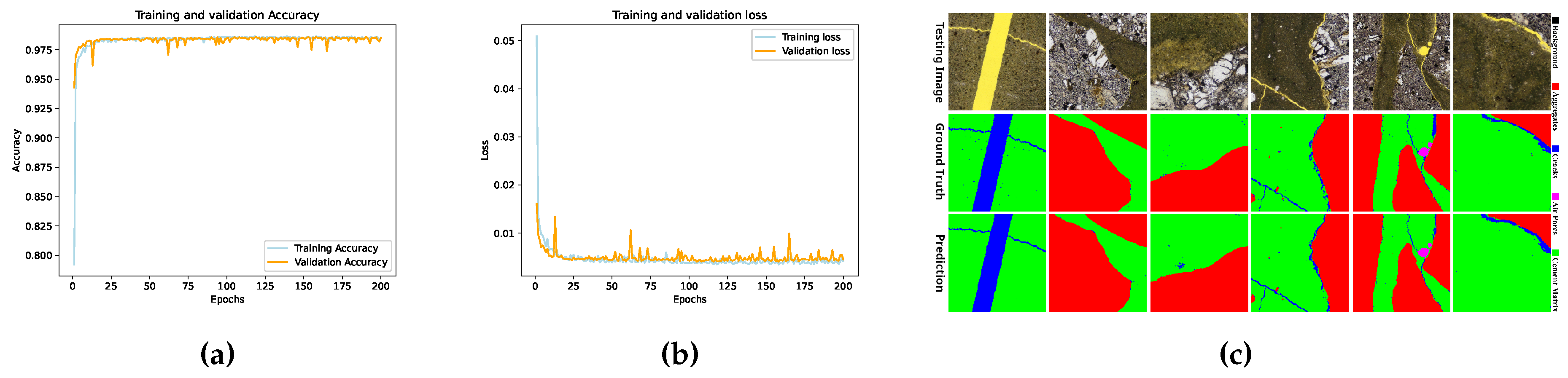
Figure 5.
Segmentation of 2D CT slices through heuristic image analysis. (a) Preprocessed CT slice after beam hardening correction. (b) Annotation mask for cracks, air pores, and cement matrix. (c) Segmentation of aggregate instances via SAM and logical operations to exclude mislabelling. (d) Superimposed multi-label annotation mask for semantic segmentation.
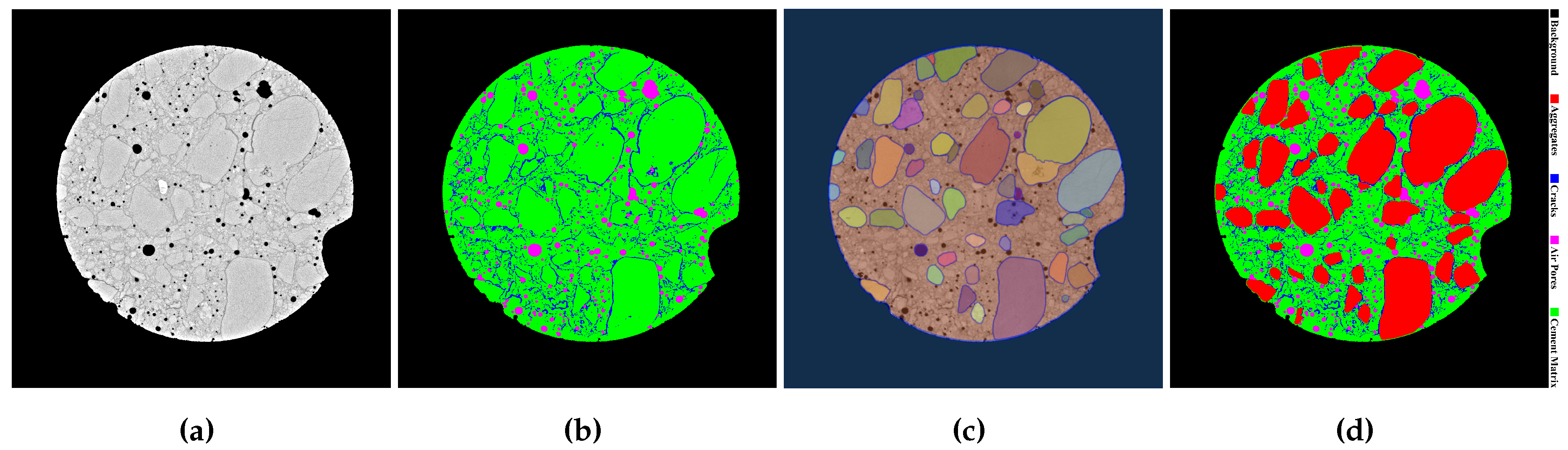
Figure 6.
Learning Curves of retrained Attention Residual UNet on the CT Dataset. (a) Accuracy Curves for training and validation sets. (b) Loss Curves for training and validation sets. (c) Inference results of the trained DNN on some validation samples.
Figure 6.
Learning Curves of retrained Attention Residual UNet on the CT Dataset. (a) Accuracy Curves for training and validation sets. (b) Loss Curves for training and validation sets. (c) Inference results of the trained DNN on some validation samples.
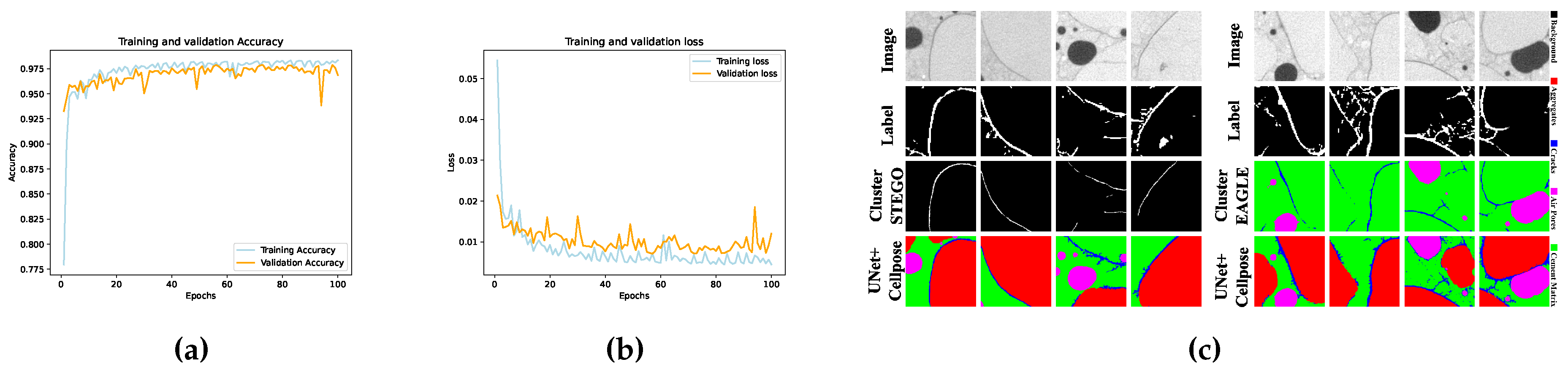
Disclaimer/Publisher’s Note: The statements, opinions and data contained in all publications are solely those of the individual author(s) and contributor(s) and not of MDPI and/or the editor(s). MDPI and/or the editor(s) disclaim responsibility for any injury to people or property resulting from any ideas, methods, instructions or products referred to in the content. |
© 2025 by the authors. Licensee MDPI, Basel, Switzerland. This article is an open access article distributed under the terms and conditions of the Creative Commons Attribution (CC BY) license (http://creativecommons.org/licenses/by/4.0/).
Copyright: This open access article is published under a Creative Commons CC BY 4.0 license, which permit the free download, distribution, and reuse, provided that the author and preprint are cited in any reuse.


