
Submitted:
20 December 2025
Posted:
22 December 2025
You are already at the latest version
Abstract
The Greater Caribbean manatee is classified as vulnerable, yet the lack of data related to population status in the Costa Rican Caribbean severely hinders conservation policy due to limited ecological knowledge. This study aims to address this challenge by refining a pipeline for the automated manatee count method to enhance classification robustness and efficiency for accurate spatial and temporal density estimation. The bioacoustics analysis consists of a deep learning manatee call detector and an unsupervised individual manatee counting. Methodologically, we implemented an offline feature extraction strategy to avoid a substantial initial computational bottleneck, measured at almost 13h, required to convert 43,031 audio samples into labeled images. To mitigate the high risk of overfitting associated with class imbalance, common in bioacoustic databases, a bootstrapping method was applied post-data splitting, generating a labeled dataset of 100,000 spectrograms. Transfer learning with the VGG-16 architecture yielded superior results, achieving a robust mean 10-fold cross-validation accuracy of 98.94% (±0.10%) and normalized F1-scores of 0.99. Furthermore, this optimized fine-tuning was rapidly executed in just 22min and 36s. Subsequently, the unsupervised individual manatee counting utilized k-means clustering on the top three music information retrieval descriptors along with dimensionality reduction, successfully segregating detected calls into three acoustically distinct clusters, likely representing three individuals. This performance was validated by a silhouette coefficient of 79.03%. These validated results confirm the refined automatic manatee count method as a robust and scalable framework ready for deployment on Costa Rican passive acoustic monitoring data to generate crucial scientific evidence for species conservation.
Keywords:
acoustic individual counting
; bioacoustics
; deep learning
; feature extraction
; kernel density estimation
; machine learning
; manatee call detection
; music information retrieval
; passive acoustic monitoring
; transfer learning
1. Introduction
The sirenians, also known as sea cows, are a group of marine mammals whose populations have been declining annually. They are listed as threatened worldwide, with some subspecies experiencing regional functional extinction [1,2,3,4,5], such as the dugong populations (Dugong dugon) in China [6,7] and Japan [8]. A subspecies of the American manatee, the Greater Caribbean manatee (Trichechus manatus manatus) has a conservation status of vulnerable [9]. This herbivorous marine mammal is rarely observed off the Caribbean coast in Costa Rica, and its population status is unknown [1,10]. It has been affected by anthropogenic activities, like poaching, fishing, boat collisions, water pollution, and ecosystem degradation [1]. The Greater Caribbean manatee was declared a national symbol of underwater fauna in Costa Rica in 2014, but the conservation regulations for this marine mammal are still scarce due to limited ecological knowledge around the species [1,10].
The 14th sustainable development goal (SDG), denoted as Life Below Water and developed by the United Nations (UN), emphasizes increasing scientific knowledge and building research capacity to support the conservation of marine biodiversity, which serves as an indicator of healthier oceans [11]. Hence, collecting and analyzing scientific evidence would justify establishing and implementing conservation actions to protect the manatees in coastal communities of Costa Rican Caribbean [1,12]. Although these mammals have a considerable size, monitoring their movements is challenging because they spend most of their life underwater. [10,13]. Sirenians emit calls for communication between cow-calf pairs and during social interactions [12,13]. Therefore, acoustic surveys emerge as a promising alternative to traditional manatee monitoring based on visual evidence [10,12,14,15,16,17].
The identification of marine mammals throughout the analysis of the underwater sounds collected in audio recordings is denoted as passive acoustics monitoring (PAM), which is a useful strategy to gain insights about species abundance, temporal, and spatial distribution without visual observations [13,14,15,16]. PAM involves the deployment of one or more hydrophones to capture marine mammal sounds in audio recordings that range from days to months [14,15]. This generates long-term databases that traditionally require manual annotation by visual scanning or audible identification for bioacoustics analysis [16].
Nevertheless, this labor-intensive task becomes unfeasible, so computational solutions powered by advanced computing that combines artificial intelligence (AI) and high-performance computing (HPC) units to automate the audio recordings analysis for studying the presence of target species with minimal human supervision in long-term recordings [14,15]. Hence, our research endeavors to advance marine conservation by developing enhanced AI-driven applications that facilitate the efficient and automated analysis of PAM recordings. These tools will enable high-confidence predictions of manatee presence and density estimates, significantly enhancing our ecological knowledge about the Greater Caribbean manatee in our country, which could be extended to other marine mammals.
1.1. Related Work
The current literature reveals that traditional AI solutions for detecting and classifying single and multiple types of marine mammals, especially cetaceans, rely on machine learning (ML) algorithms [14,15,18]. For example, humpback whale (Megaptera novaeangliae) acoustic detection has been achieved using the support vector machine (SVM) as a binary classifier to distinguish between song and non-song sounds in audio samples [14,15,18]. Furthermore, a hidden Markov model (HMM) has been implemented to identify both humpback whale calls and dolphin signature whistles, demonstrating its versatility in multi-species acoustic analysis [14,15,18]. Alternatively, an unsupervised approach employing a Gaussian mixture model (GMM) has proven effective in classifying vocalizations from various dolphin species and toothed whales, highlighting the potential of unsupervised methods in complex bioacoustic datasets [14,15,18]. Utilizing GMMs, a multi-classifier accurately has categorized vocalizations of Arctic marine mammals into seven classes: five whale species, walruses, and background noise [19].
Recently, the deep ML or deep learning (DL) has shown an impressive throughput for bioacoustics analysis using different types of deep neuronal network (DNN) models [15,18]. A beluga whale (Delphinapterus leucas) detector implemented an ensemble model of DNNs by training four distinct convolutional neuronal network (CNN) architectures, specifically designed for the classification of whistles and moans [20]. For the binary classification of humpback whale songs, a CNN framework incorporated active learning, where the outputs of candidate models were utilized to guide subsequent annotation efforts, thereby enhancing classification accuracy after training the models with these guided annotations [21]. Furthermore, a multi-classifier system for cetacean whistles, encompassing 60 distinct marine mammal species, utilized a seven-layer CNN architecture to categorize the acoustic signals into six distinct whistle types [22].
However, as DNNs scale in depth to enhance classification throughput by increasing model complexity, the gradients propagated during supervised training can diminish to near-zero values, compromising the learning at earlier layers [23]. To mitigate this vanishing gradients issue, residual learning bypasses layers and directly adds the input to the output through skip connections. The residual neuronal network (ResNet) architecture leads to superior performance classifying 32 species of marine mammals compared to CNNs [23]. But it is crucial to acknowledge that ResNet, like many DL models, are susceptible to overfitting, particularly when they are trained on small datasets, as commonly occurs within PAM databases [18]. This means that there are not enough labeled audio samples to train these architectures due to the time-consuming nature of manual data labeling [15].
A solution to reduce the risk of overfitting and improve generalization in automated bioacoustics analysis, even with limited labeled data, is transfer learning. This DL technique leverages pre-trained models initially trained on large, diverse datasets. The model benefits from the pre-learned features by fine-tuning these models on the smaller, specific dataset. For classifying three species of marine mammals, non-biological noise, and ambient noise, Thomas et. al. (2019) employed transfer learning upon the pre-trained weights of CNN models, such as ResNet-50 and VGG-19 [24]. A further contribution utilized transfer learning, employing two pre-trained AlexNet models, to achieve both sound detection and multi-class classification of three marine mammal species: killer whales, long-finned pilot whales, and harp seals [25].
Recent studies concerning sirenian bioacoustic analysis have predominantly leveraged DL methods for detecting manatee vocalizations, utilizing various architectural approaches [26]. For instance, a binary classifier for Amazonian manatee (Trichechus inunguis) populations incorporated a CNN architecture, alongside an active learning methodology and data augmentation to address limited training data, relying on manual inspection to increase labeled samples [27]. To identify the Greater Caribbean manatee in the western Caribbean region of Panama, a data-driven scheme implemented binary classification using two CNN configurations: a linear architecture with a fixed kernel size and a pyramidal architecture with an increasing kernel size [28].
However, this specific system did not incorporate data augmentation or balancing techniques, potentially limiting generalization and increasing the risk of overfitting [28]. For the binary classification of African manatee (Trichechus senegalensis) presence, a transfer learning approach was employed, leveraging a pre-trained GoogLeNet network to mitigate the paucity of labeled data, although without implementing individual counting [29]. Another transfer learning strategy considered a two-stage CNN ensemble for manatee sound classification [30]. This architecture first discriminated between genuine manatee vocalizations and background noise, followed by a five-class categorization of call types [30]. EfficientNet served as the feature extractor, pre-trained on a zoo-based dataset and subsequently fine-tuned on data from additional zoo locations [30].
Finally, an automated system for Greater Caribbean manatee identification and population estimation on the Caribbean coast of Costa Rica employs a transfer learning approach with VGG-16 as a feature extractor, fine-tuned on a labeled dataset of Florida manatees (Trichechus manatus latirostris) [26]. Subsequently, an unsupervised k-means (KM) method, initialized using the expectation-maximization (EM) algorithm, was applied to group acoustic features, effectively combining DL models for binary call detection with ML clustering to predict individual call origins [26]. However, the authors reported considerable challenges within real-world recordings due to background noise interference (e.g., boat noise and splashing) and overfitting that might be introduced by data imbalance and the limited size of the training dataset [26].
Therefore, this study addresses the limitations of the automatic manatee count method (AMCM) framework by enhancing binary classification robustness, pipeline scalability, and clustering precision within complex marine soundscapes [26]. We introduce critical improvements to the time-frequency preprocessing and image generation stages, alongside enhance prediction reliability measures and the evaluation of DL architectures. To mitigate overfitting and ensure long-term inference stability, the methodology integrates strategic data balancing, bootstrapping-based augmentation, and rigorous cross-validation. These optimizations provide a standardized basis for accurate population and density estimations in the Costa Rican Caribbean coast. This research could establish a validated, high-performance framework designed to inform evidence-based conservation policies for environmental authorities. By improving the monitoring of the Greater Caribbean manatee, this system would promote ecological awareness and supports targeted protection efforts within coastal communities.
2. Materials and Methods
The computational design of the proposed solution builds upon previous efforts, specifically the AMCM pipeline [26]. In its generality, this system is structured around two main modules for the bioacoustic analysis of Greater Caribbean manatee calls: the manatee call detection (MCD) and the individual manatee counting (IMC). The MCD module implements a binary classifier based on a comprehensive DNN framework for discriminating between genuine and false manatee calls in acoustic recordings, incorporating a novel functional block to improve the estimator’s behavior under challenging real-world conditions. The IMC module employs ML clustering techniques to categorize the detected calls based on music information retrieval (MIR) attributes without requiring labeled data from the monitored population. Regarding the clarity and coherence enhancement of this manuscript, a generative AI tool, precisely Gemini Flash 2.5 variant, was used in select paragraphs to draft and refine text from author-provided outlines, with all outputs critically reviewed and revised by the authors for accuracy and content responsibility.
2.1. Training and Testing Database
To train and validate the MCD model, a comprehensive database was constructed by integrating five diverse PAM datasets, totaling 43,031 labeled audio samples. These samples originated from various acoustic platforms, including autonomous wild recorders, biologging tags, and controlled recordings from manatees under human supervision, encompassing a range of sampling rates and durations [26,31]. Beyond existing sources, the repository was expanded to include recordings from Florida manatees (Trichechus manatus latirostris) and african manatees (Trichechus senegalensis) from Nigeria and Cameroon. This inclusion is justified by the structural similarities between these vocalizations and those of the Greater Caribbean manatee [32]. The integrated dataset consists of WAV files categorized by binary labels: false vocalization (28,765 instances) and true vocalization (14,266 entries), reflecting a significant class imbalance of approximately between the target categories.
For the experimental validation of the refined AMCM pipeline, we utilized labeled field recordings sourced from Bocas del Toro in the Panamanian Caribbean. Although these recordings provided a ground-truth count of the expected manatee vocalizations per audio sample, the exact temporal occurrences of individual calls were not pre-identified. Despite this condition, the experimental dataset allowed for a robust evaluation of the detection functionality of the updated MCD module within a real-world unseen experimental context [26]. Specifically, we established a dedicated verification directory containing these labeled recordings to facilitate the system’s performance assessment. While the samples varied in duration and length, they maintained a standardized sampling rate of 96 ensuring methodological consistency with prior research and providing a stable baseline for the inference evaluation of the updated model architecture [26].
2.2. Feature Extraction and Data Pre-Processing
Following standard workflows for marine mammal classification, the MCD incorporates an audio feature extraction (FE) stage to transform raw 1-dimensional (1D) waveforms into discriminative 2-dimensional (2D) spectral representations [15]. Our study applied successive fast Fourier transform (FFT) operations with a window size of 1022 and a 25% overlap to achieve time-frequency conversion. The core pipeline involved resampling signals to a uniform 44.1nd applying logarithmic interpolation to rescale spectral magnitudes, with cutoff margins set at 80% of the upper and lower frequency boundary values. The operation effectively reassigned the linear frequency bins generated by the FFT onto a logarithmic scale, which better approximated the perceived harmonic structure of biological signals. To enhance tonal clarity and isolate harmonic patterns, a robust denoising strategy was implemented. This involved a 4th order high-pass filter with a 2utoff frequency to suppress low-frequency ambient interference. Furthermore, spectral gating was utilized for noise reduction and harmonic sound source separation, ensuring the resulting spectrograms emphasized the unique acoustic footprints required for effective manatee call detection.
Traditional FE methodologies rely on classical signal processing, such as onset detection and padding, to determine time occurrence for enforcing uniform segment lengths within unconstrained acoustic data [26]. In contrast, this study implements a comprehensive image processing stage that directly generates 2D spectrograms on a dB-scale, transforming audio into a visual format optimized for DL models. These representations were further processed using horizontal flipping and pixel-interpolation resizing before being converted into 128×128×3 RGB color images via color-space conversion (CSC). This workflow encapsulates acoustic signatures into discrete spectral images stored in 8-bit unsigned integer ( format to ensure architectural compatibility and standardized pixel intensity ranges. To address the computational bottleneck of the WAV-FE loop, an offline processing strategy was implemented, pre-converting audio samples into standardized JPEG formats. This approach significantly reduced execution overhead during the benchmarking of various DL architectures. To maintain data integrity, a centralized transcription file for the resulting database was generated to map each stored image to its corresponding ground-truth label.
2.3. Data mining and Augmentation
By analyzing the resulting data structure of the spectrogram database transcription from the FE workflow, the labeled spectrograms were transformed into a multi-dimensional array for DL integration. Preliminary data processing involved vectorization and the evaluation of scaling techniques—such as min-max normalization and standardization—alongside the numerical conversion of categorical labels. Following the removal of not-a-number (NaN) values, explicit external scaling was omitted; this shift was justified by the inclusion of batch normalization layers within the DL architectures, which effectively regulate input distributions and mitigate internal covariate shift. To maximize throughput for GPU-accelerated processing, both feature vectors and class labels were cast to 32-bit floating-point precision (. This configuration maintains high computational efficiency and numerical consistency while balancing memory management with spectral resolution. Furthermore, raw class labels were mapped using both ordinal and one-hot encoding schemes, ensuring full compatibility with the specific loss functions and architectural requirements of the classification models detailed in subsequent sections.
Furthermore, the complete dataset was partitioned into three distinct sets using a pre-defined ratio to evaluate model performance and generalization capability. We employed random stratified sampling to divide the data into training (70%), testing (20%), and validation (10%) sets from the complete dataset, ensuring the proportional representation of classes in each split. To address the class imbalance found in each data split, we incorporated data augmentation—a critical step in mitigating bias and improving model generalization—to increase the size and diversity of our labeled data splits. Specifically, we utilized a non-parametric bootstrapping method to generate new, synthetic spectral images by resampling existing ones from the original labeled database. This technique was crucial for synthesizing a larger, balanced number of spectrograms across both positive and negative classes, thereby improving model robustness [33]. The non-parametric bootstrap algorithm is a statistical technique used to evaluate the accuracy or distribution of a parameter estimator, especially in signal processing applications where standard asymptotic methods may not be valid due to small sample sizes or time constraints [33].
Essentially, bootstrapping is a powerful, computer-based method that replaces theoretical analysis with a considerable amount of computation, simulating the repetition of the experiment by randomly reassigning observations thousands of times [33]. Beginning with an original random sample (), the empirical distribution, , is constructed, assigning equal mass () to each observation. A bootstrap resample () is then drawn from randomly with replacement, ensuring contains n items and is likely to include repeats from the original set. A parameter estimate () is calculated from this resample, and this resampling and recalculation process is repeated a large number of times (e.g., N or B times) to generate a collection of bootstrap estimates . The distribution of these estimates approximates the actual sampling distribution of the estimator, , which can then be used to calculate statistics like variance or to construct confidence intervals [33].
To handle properly large and complex data arrays resulting from data augmentation, our system provided an option for data pipelining to reduce input-output bottlenecks of the labeled datasets. Furthermore, we integrated exploratory data analysis (EDA) throughout the data mining phase to derive valuable insights regarding the effects of audio preprocessing on both types of spectral image samples [26]. This included analyzing data distribution across categories and visualizing the samples transformed in the WAV-FE module to observe the highlighted patterns within the images associated with the tonal calls of the target species.
2.4. Deep Learning Methodology
Achieving high performance in real-world scenarios is critical for the MCD module across all its operational stages, demanding optimization in both predictive accuracy and computational execution time. Consequently, we conducted a comprehensive comparative evaluation (i.e., benchmarking) between custom DL architectures and pre-trained models for the MCD module, considering the proposed changes in the WAV→JPEG transformation. The model yielding the best performance metrics was subsequently selected for deployment. These supervised and transfer learning experiments were executed utilizing the HPC infrastructure of the Kabré supercomputer. This platform incorporates powerful GPUs, specifically NVIDIA L40S and Tesla V100 units, which were leveraged for model training, rigorous evaluation, and subsequent high-throughput inference testing.
To maximize the computational throughput of the HPC infrastructure, mixed-precision training was implemented across the training and inference workflows. This strategy utilized 16-bit floating-point precision ( for compute-intensive tensor operations while selectively retaining or critical variables, such as loss scaling and master weights, to maintain numerical stability and prevent gradient underflow. Comprehensive hardware specifications—including CPU architecture, memory capacity, and the operating system environment—are detailed in Table 1. In contrast, the IMC module involved training an unsupervised ML model on a reduced observation dataset within a low-dimensional feature space. Given the significantly lower computational complexity of this stage, the IMC module operated efficiently on the CPUs of the Kabré supercomputer. The successful execution of this module without specialized GPU acceleration underscores the flexibility of the pipeline and its capacity to scale across heterogeneous hardware tiers according to the specific demands of each analytical phase.
The refined MCD implementation was developed within a supervised DL framework, ensuring methodological continuity with prior research [26]. To determine the optimal DL configuration for MCD, we benchmarked two architectural paradigms: custom-designed CNN and ResNet configurations—noted for their efficacy in marine bioacoustics [23]—and transfer learning utilizing pre-trained architectures such as VGG-16, VGG-19, and EfficientNet. These pre-trained models were strategically selected to address the data scarcity challenges inherent in bioacoustic monitoring, leveraging their demonstrated capacity to enhance classification accuracy in Sirenian vocalization studies [13,26,30].
For general model building parametrization across both DL approaches, the input layer of these models was consistently shaped as 128×128×3, corresponding to the dimensions of the input spectral images. The output layer size was fixed at 2 to align with the binary encoding scheme of the target labels. Hyperparameter tuning was initially performed using a brute-force approach in both supervised and transfer learning methodologies. Suitable hyperparameter configurations were selected through a focused series of trial-and-error adjustments, guided by rigorous performance evaluation across train-validation splits and cross-validation metrics. This comparative analysis against the experimental results of previous work informed the final architectural decisions for both learning approaches [26].
The custom-designed and configurable architecture for the CNN model was comprised of four hidden layers, each utilizing a ReLU activation function and sequentially followed by max-pooling and batch normalization layers. The convolutional layers employed a spatial dimension of 3×3 and initiated with 16 filters, which subsequently doubled per layer (i.e., 16→32→64→128). To mitigate overfitting, regularization () was applied to the convolutional layers, and a dropout layer with a magnitude of 0.7 was included before the final classification block. This consisted of a dense, fully-connected, layer with 64 artificial neurons, feeding into the final binary Softmax output layer. For model compilation, the Adam optimizer was utilized with a learning rate of 1, employing binary classification metrics.
Regarding the transfer learning approach, the model ensemble was constructed upon either a pre-trained VGG-16, serving as the baseline from previous work [26], or VGG-19 architecture, both initialized with weights trained using ImageNet database [34]. The pre-trained convolutional base was augmented with a custom classification head, consisting of a single fully-connected layer with 128 units, followed by the requisite hidden and final output activation layers. Shared generalization parameters across both DL methodologies, consistent with custom model configurations, included the Adam optimizer, regularization (=0.001), and a dropout magnitude of 0.7. Training was conducted in two distinct sequential stages: the first stage involved the pre-trained model implementation, where the base layers were predominantly frozen, but 25% of the terminal convolutional layers were strategically unfrozen for training with a learning rate of 1. Subsequently, the second stage, the so-called fine-tuning, began, where all base layers of the model ensemble were unfrozen and trained with a significantly reduced learning rate of 1 to facilitate complete and subtle adaptation to the spectral characteristics of the manatee spectrogram data.
Model training for any DL methodology was configured for a maximum of 600 epochs, utilizing a consistent batch size of 128. To prevent overfitting and avoid unnecessary retraining, we employed two critical control strategies: early stopping and model checkpointing. Early stopping halts the training process when the validation loss begins to degrade, while model checkpointing saves the model state exclusively, as a Keras format file (.keras), when the monitored metric improves. Specifically, the early stopping mechanism was implemented on both supervised and transfer learning models, monitoring the validation loss and requiring a minimum improvement delta of 0.0001 over a patience of 10 consecutive epochs. Following training, the final model object was restored to the optimal parameter set recorded on disk, thereby discarding the parameters of the last, potentially overfitted, epoch. Finally, the methodology retrieved visual outputs of the manatee call classification alongside the model’s binary classification metrics as a final EDA step of the MCD module, utilizing informative plots about the historic progress of the model training and validation.
2.5. Model Evaluation and Inference
Once the DL model was trained, our computational solution performed the MCD evaluation to compute predictions with a portion of the labeled 2D spectrograms for verifying the model capabilities with unknown samples [26]. The binary classification performance was evaluated using cross-entropy loss, which measures the discrepancy between the predicted and actual class distributions. This evaluation involved the categorization of predictions into a true positive (TP), representing an accurate positive class prediction; a false positive (FP), indicating a missed detection; a true negative (TN), denoting a correct non-positive class prediction; and false negative (FN), signifying incorrect non-positive class predictions. To rigorously assess performance, a suite of classification metrics was employed [26]. Accuracy (Eq.1) provided an overall measure of correct predictions between both categories:
Precision and recall (i.e., sensitivity) were calculated for both true and false vocalizations to evaluate detection purity and completeness, respectively:
The F1-score, defined as the harmonic mean of precision and recall, served as a balanced metric to evaluate the model’s robustness under potentially imbalanced data conditions:
To assess the model’s discriminative power, the area under the curve (AUC) of the receiver operating characteristic (ROC) curve was calculated by evaluating the TP rate against the FP rate across various decision thresholds. This metric provides a robust measure of the classifier’s ability to distinguish manatee vocalizations from background noise independently of the chosen threshold. To rigorously evaluate generalization and mitigate overfitting, a k-fold cross-validation strategy was implemented. The dataset was partitioned into mutually exclusive folds of equal size, with the model undergoing ten iterations of training on folds and validation on the remaining held-out fold [18]. By rotating the validation set so that each fold was utilized for testing exactly once, we obtained unbiased estimates of training and validation errors. This comprehensive framework ensures that performance metrics accurately reflect the model’s capacity to generalize to unseen acoustic data [18].
During the model inference stage, the audio-image FE pipeline was adapted to process prolonged, unlabeled real-world recordings while maintaining strict parity with the training configuration [26]. The process begins with loading raw acoustic data, followed by resampling and temporal segmentation into uniform one-second (1 slices. These segments undergo an online FE routine—incorporating denoising, logarithmic interpolation, and CSC—to generate an array of spectral images identical in structure to those used during the training phase. Data mining procedures were consistently applied to prepare these images for model ingestion, ensuring localized signal integrity. This involves vectorizing the multidimensional spectrogram array and casting the resulting features to recision. By utilizing optimized data pipelining, the system achieves high-throughput processing, allowing for the efficient transformation of raw field recordings into standardized input tensors compatible with the trained DL architectures.
Once the FE phase was done, the system instantiated and compiled the deep DL architecture, loading the optimized weights to initiate inference. Predictions were generated by iteratively processing data batches through a dedicated pipeline tailored to each experimental recording. During this routine, the indexed spectrogram array was fed into the model to obtain class-specific posterior probabilities, which were subsequently archived in a comprehensive transcription file. To refine the results and mitigate FPs, a selection threshold was applied to the prediction confidence scores. The post-processing step served as a critical filter to distinguish valid manatee vocalizations from pervasive environmental background noise. Specifically, only detections exceeding a probability threshold of 0.5 for the positive class were classified as genuine calls. This rigorous validation criterion ensures that the resulting census and spatial-temporal density estimations are based on high-confidence acoustic events.
As a fundamental component of the EDA for the inference stage, a 1D signal representation was generated for each input sample. This time-domain visualization was annotated with temporal markers indexing the specific instances where the model identified potential manatee vocalizations [26]. To augment this analysis, the system implemented a random sampling routine to visualize batches of spectral images, each labeled with its segment index, predicted class, and associated confidence score. This visual framework facilitated qualitative assessment of model performance on unseen data, providing essential insights into generalization capabilities within complex marine acoustic environments. Furthermore, this dual-representation approach enabled the visual verification of TPs and the identification of FPs, thereby streamlining the process for subsequent expert validation and iterative model refinement [26].
To validate the behavioral performance of the MCD module on unseen data, inference outcomes were evaluated using an experimental repository of real-world field recordings [26]. This verification process leveraged apriori knowledge regarding the expected number of manatee calls within each recording to benchmark the model’s predictive accuracy. By comparing the predicted call count against the expected ground truth, the model’s generalization capabilities were quantified. The precision of these detections was measured using a modified experimental error metric that quantifies the deviation of model estimations from the expected values:
2.6. Unsupervised Learning
Following the inference phase across the experimental recordings, a comprehensive bioacoustics analysis was performed on each manatee vocalization detected to compute MIR descriptors. This analysis served as the specialized FE stage for the IMC module. Initially, an adaptive time-domain denoising routine was applied to each identified call to improve the isolation of harmonic components. This preprocessing pipeline integrated high-pass filtering, signal normalization, and spectral noise reduction to emphasize the fundamental frequency structure of the vocalizations.
Subsequently, the system performed a numerical characterization of every call identified as valid according to the established confidence threshold. For each detection, 11 distinct MIR attributes were computed and appended to a data structure, forming a detailed transcription file for the testing dataset. These extracted features—which constitute the acoustics FE output for vocalizations identified by the MCD module—included the fundamental frequency (), bandwidth (BW), spectral centroid, spectral roll-off, spectral contrast, spectral flatness, zero-crossing rate (ZCR), kurtosis, skewness, and the root-mean-square (RMS) value. This high-dimensional feature set provides a robust quantitative foundation for the subsequent unsupervised clustering and population estimation processes [26].
Consistent with the IMC methodology established in prior research, the preparation of unlabeled MIR data for clustering remains fundamentally uniform [26]. In the current study, we utilized a structured dataset for MIR data-framing, comprising manatee vocalization observations paired with a comprehensive suite of MIR descriptors across both the temporal and spectral domains. From this structure, the IMC module extracted a MIR data array for vectorization. An essential data mining phase preceded the analysis, involving a rigorous inspection for invalid feature values to identify and remove observations containing NaN entries. These instances were frequently associated with potential FPs that remained undetected during the initial MCD inference stage.
Following data cleaning, we applied feature scaling via min-max normalization to constrain the feature values within the range of 0 to 1, ensuring feature value parity and preventing descriptors with larger numerical scales from dominating the model training. To further refine the feature space and optimize the subsequent unsupervised ML modeling, a multi-stage dimensionality reduction strategy was implemented. Initially, feature selection was performed by calculating the Gini importance derived from fitting a random forest (RF) classifier with 100 decision trees (DT) to the MIR feature map [26]. This process facilitated the identification and isolation of the top-three most relevant acoustic descriptors, effectively reducing noise and computational complexity while preserving the most discriminative information for the clustering algorithm.
To further streamline the MIR feature space, we applied either principal components analysis (PCA) or non-negative matrix factorization (NMF) to compress the multidimensional acoustic descriptors into a two-dimensional representation [26]. These dimensionality reduction techniques were strategically combined to mitigate the curse of dimensionality within the dataset, thereby optimizing the input for the subsequent clustering and population estimation stages. For comparative analysis and validation against established benchmarks, we replicated the clustering algorithm selection strategy employed in our previous research [26]. The configuration of the IMC module—including the parameters selection of the KM-EM method and the reduction of the feature space via PCA—was empirically tuned through a systematic trial-and-error approach, maintaining methodological consistency with both the MCD model development and our prior work [26].
As an EDA step for the IMC module, a correlation matrix was calculated to quantify relationships between MIR attributes, effectively identifying latent dependencies and feature redundancies. Complementary bivariate scatter plots were utilized to visualize the distribution of potential individual manatees across paired MIR descriptors, providing a graphical assessment of feature patterns derived from both controlled and real-world acoustic datasets [26]. To enhance interpretability, the visualization incorporates kernel density estimation (KDE) to map the density of calls within the feature space. This method highlights regions of high data concentration and offers a clear representation of cluster separation, which reflects the distinct temporal and spectral signatures associated with individual manatees.
Structured transcription files archived identified vocalizations with their MIR attributes and cluster assignments to facilitate downstream ecological and population modeling [26]. The unsupervised IMC module was evaluated using two primary metrics. The inertia score—representing the within-cluster sum of squares—served as the objective function for KM-EM optimization. The optimal cluster count, k, was identified via the elbow method, where the inflection point indicates maximum compactness. This parameter corresponds to the number of distinct individuals based on unique MIR signatures [26]. In addition, the silhouette score was employed to quantify cluster cohesion and separation by quantifying the similarity of an object to its own cluster relative to other clusters. This metric ranges from to 1, where higher values indicate well-defined groupings. The score is calculated as follows:
where N is the sample total, denotes the mean intra-cluster distance, and represents the mean distance to the nearest neighboring cluster. This dual-metric approach ensures the objective validation of the acoustic segregation of individual manatees.
rmsRMSroot-mean-square
3. Results
Processing the complete labeled database via online WAV-FE required substantial time, taking 12 4 and 10n the L40S unit for training and validation modes of the MCD module. This motivated the selection of the offline FE for mitigating the computational bottleneck and accelerate subsequent DL benchmarking. This involved pre-generating and storing the spectral images as JPEG files along with its corresponding transcription. The image-FE step then loaded the data structure from the labeled spectrograms, yielding a high-dimensional array containing raw time-frequency data, characterized by dimensions of 43,031×128×128×3.
Following the data mining phase, the dataset was vectorized into a high-dimensional array of 43,031×49,152. External scaling was bypassed at this stage, as input normalization was deferred to the internal layers of the DL architecture. Target classes extracted from the database transcription were encoded into a binary representation, resulting in a labels array of 43,031×2, where and denote false and true vocalizations, respectively. To optimize the balance between computational throughput and memory management, both the feature and label vectors were cast to recision. The dataset was partitioned using random stratified splitting to ensure proportional class representation across all subsets. The training set (30,121 samples) comprised 20,135 false and 9,986 true vocalizations; the testing set (8,607 spectrograms) included 5,754 false and 2,853 true vocalizations; and the validation set (4,303 images) contained 2,876 false and 1,427 true vocalizations, where this distribution preserves the inherent class imbalance of ∼50% across the MCD module.
To mitigate the inherent class imbalance present in the original dataset and enhance model generalization for each DL methodology under study, the bootstrapping augmentation process created balanced class distributions, resulting in a complete synthetic database totaling 100,000 samples. This final dataset was subsequently partitioned into balanced subsets: 70,000 samples for training, 20,000 samples (10,000 per class) for testing, and 10,000 samples (5,000 per class) for validation. All these balanced splits were efficiently integrated into their corresponding ata pipelines for optimized model feeding and computational efficiency.
As part of the EDA actions on the WAV-FE results, Figure 1 depicts a sample of data batches, extracted from the resulting data pipeline, labeled with the ordinal encoding scheme of the expected labels, after the completion of the data mining stage. These batches are composed of randomly selected spectrograms, rendered as RGB color images of 128×128×3 dimensions, where the x-axis denotes the height and the y-axis represents the width, both measured in pixels, allowing the observation of distinct high-frequency harmonical patterns related to positive samples. The model construction and configuration of the custom CNN model resulted in a network with 106,306 trainable parameters. Figure 2 shows the corresponding metrics of the supervised model training once the early stopping is done after 27 and 51.33 where the training process halted at the 105th epoch. Concurrently, the model checkpointing callback ensured that the optimal weights—achieved at the 95th epoch model—were saved for subsequent evaluation.
To evaluate the generalization performance on a per-class basis, the saved model was reconstructed and loaded to compute key classification throughput on the testing or evaluation split. Part of the evaluation model results are summarized in Table 2, which presents the confusion matrix detailing the percentages of correct detections and incorrect estimations for both classes, which represent in counts: 9,857 TNs and 143 FNs for false vocalizations, and 9,736 TPs and 264 FPs for true vocalizations. The overall binary accuracy (Eq. 1) achieved was 97.93%, with a corresponding binary cross-entropy loss of 6.70%, where the AUC-ROC was calculated to be 97.96%. Further insights into the model’s per-class performance are provided in Table 3, which presents the comprehensive classification report for the loaded CNN model by computing the binary classifier evaluation using Eq. 2, Eq. 3, and Eq. 4. The report highlights the model’s high reliability, achieving normalized F1-scores of 0.98 for both positive and negative instances.
Concurrently, Figure 3 offers an inference EDA tool, depicting the model’s predictions on a sample data batch from the testing split. This visualization serves to confirm that the predicted outcomes with the associated confidence scores, align accurately with the expected binary labels. Following the final model evaluation, the 10-fold cross-validation procedure demanded a duration of 8 24 and 49.82 The mean performance metrics across all ten folds were then computed, yielding a mean binary accuracy of 97.89% with a standard deviation of ±0.06% and a mean binary cross-entropy of 5.84%.
Regarding the model ensemble for the transfer learning approach, the initial backbone, with base layers predominantly frozen, involved 65,922 trainable parameters for both pre-trained VGG-16 and VGG-19 architectures. Subsequently, the fine-tuning stage involved unfreezing all base layers, resulting in a larger parameter count for optimization: approximately ∼7.15 million parameters for VGG-16 and ∼9.50 million parameters for VGG-19. The complete fine-tuning process required a total time of 22nd 36or VGG-16, and 16nd 48or VGG-19. Figure 4 visually validates the transfer learning process by plotting the binary accuracy and cross-entropy loss as a function of training epochs for both pre-trained models. The plot highlights the specific epochs at which the fine-tuning phase was initiated and terminated by early stopping. For VGG-16, fine-tuning began at the 84th epoch and terminated at the 135th epoch. This phase for VGG-19 was initiated at the 232nd epoch and concluded at the 266th epoch.
Upon storing the final optimized weights after fine-tuning, the large-scale VGG-16 model demonstrated superior performance, yielding an overall binary accuracy of 98.53%, a binary cross-entropy loss of 5.51%, and an AUC-ROC of 98.54%. The VGG-19 model achieved highly comparable metrics, including an accuracy of 98.35%, loss of 5.52%, and AUC-ROC of 98.36%. Table 4 presents the detailed confusion matrices for both models. For the VGG-16 classifier, performance included 9,901 TNs and 9,807 TPs, resulting in 99 FNs and 193 FPs. The VGG-19 model recorded 9,872 TNs and 9,799 TPs, with 128 FNs and 201 FPs. Further insights are provided in Table 5, which contains the binary classification report for both the pre-trained models that indicates F1-scores of 0.99 for both classes.
Figure 5 presents the visual predictions as EDA, generated by this selected pre-trained model on a sample data batch from the testing set. Considering the same spectral image data as Figure 3 for EDA, enabling direct comparison between the predictions made by the transfer learning and supervised learning approaches. Employing the same rigorous 10-fold cross-validation strategy as in prior experiments, the model evaluation provided a robust assessment of generalization capabilities for both architectures. The VGG-16 cross-validation required approximately 12 36 and 20 yielding a mean binary accuracy of 98.94% (±0.10%) and a mean binary cross-entropy of 4.28%. The VGG-19 cross-validation took 12 33 and 44nd showed slightly lower aggregated performance: mean binary accuracy of 98.50% (±0.08%) and a mean binary cross-entropy of 5.20%.
3.1. Manatee Call Detection
Following training and validation, the MCD system transitioned to a deployment phase for experimental inference. Given that this operation mode is significantly less computationally intensive than supervised training for moderate datasets, evaluations were performed on an NVIDIA Tesla V100-PCIE-32GB GPU (Table 1). This deployment considered a VGG-16 transfer learning ensemble, a selection supported by empirical performance metrics observed during the previous benchmarking phase. The VGG-16 architecture consistently yielded superior cross-validation results compared to both the custom CNN and VGG-19 ensembles. By providing an optimal balance between depth and generalization capacity, the VGG-16 model effectively outperformed alternative configurations, ensuring robust classification performance within the specific acoustic constraints of this study.
The validated MCD model was deployed for inference on an unseen testing dataset consisting of ten experimental recordings from the Bocas del Toro repository [26]. This process yielded a comprehensive transcription of results, summarized in Table 6, which contrasts ground-truth annotations against model predictions to quantify performance via the experimental inference error metric (Eq. 5). Quantitative evaluation identified 98 total predictions against a baseline of 69 expected vocalizations, exhibiting an aggregate inference error of 0.42, according to the results in Table 6. While the system demonstrated a high detection rate, the MCD module produced an average per-recording error of 0.58 (Table 6). These metrics suggest that while the model is highly sensitive to acoustic events, environmental noise or call over-segmentation may contribute to the observed variance in predictive accuracy.
Significant discrepancies between expected and predicted call counts were observed in specific samples, most notably in recording , which exhibited an outlier inference error of 1.83 (Table 6). Rigorous visual inspection of the spectral outputs revealed that many of these predicted signals were actually TPs previously missed during manual ground-truth annotation. This suggests that the model may possess a higher sensitivity for subtle vocalizations than the initial human baseline. Conversely, recording demonstrated high precision with a minor error characterized by a single FP. In this instance, the model generated 10 predictions for an expected count of 9, yielding an inference error of 0.11. Qualitative analysis via the EDA transcription confirmed that the additional detection possessed a confidence score of 0.58, yet lacked the characteristic harmonic structure of a valid manatee vocalization upon expert review.
Figure 6 provides a qualitative EDA of the model’s inference performance on the recording (Table 6), demonstrating high precision in localized MCD with an inference error of 0.17. This visualization synchronizes the time-domain signal with the corresponding batch of 1ignal segments used for inference. In this instance, the system identified 7 valid detections; although 6 calls were anticipated, two adjacent detections successfully captured a single, continuous vocalization that spanned the segment boundary. The majority of these detections yielded classification probabilities close to ∼1.00, enabling a direct correlation between the model’s high-confidence decisions and the distinct spectral signatures present in the data. This integrated visual framework effectively highlights the model’s discriminative power and its ability to maintain temporal alignment within long-term acoustic recordings. To ensure high-fidelity data logging and facilitate post-hoc sensitivity analysis, these transcriptions archived all model estimations with prediction probabilities greater than the confidence score (0.5), intentionally bypassing any possible FPs. From a computational performance perspective, the total inference duration for the entire directory—comprising 10 field recordings of heterogeneous lengths and durations—was approximately 23nd 32hen executed on the NVIDIA Tesla V100 GPU.
3.2. Individual Manatee Count
Following the MCD stage, the system executed a MIR-FE routine for every identified vocalization, extracting temporal and spectral descriptors directly from the 1D signals. This process generated 10 individual MIR transcription files, which were consolidated by the IMC module into a unified, unlabeled database. The resulting feature matrix consisted of 98 observations characterized by 11 acoustic and temporal descriptors. During the data mining phase of the IMC, 9 NaNs associated with FPs were removed, yielding a refined dataset of 89 valid observations or real TPs, summarized per sample in Table 6. The data were then vectorized and cast to recision. Finally, min-max normalization was applied to scale all features within the range , ensuring that descriptors with varying physical units contribute proportionally to the distance-based metrics employed in the subsequent clustering analysis.
The optimal number of clusters, determined to be , was identified by iteratively evaluating the inertia score across a range of potential cluster counts using the elbow method. To enhance the efficiency of the subsequent unsupervised ML phase, feature selection was initially performed utilizing Gini importance. This process identified the following descriptors: BW, spectral centroid, and spectral roll-off, resulting in an 89×3 feature data matrix. Further EDA revealed that these descriptors exhibited high-positive Pearson correlation coefficients, ranging from 0.95 to 0.98. This strong redundancy between the selected features indicated that the underlying variance could be effectively captured in a lower-dimensional space. Consequently, PCA was applied to perform dimensionality reduction, transforming the three correlated descriptors into two principal components. This transformation yielded a final 80×2 data structure that optimally preserved the variance of the original signal characteristics while facilitating more robust cluster separation.
The clustering performance was rigorously assessed through the computation of the silhouette score (Eq. 6). The implementation of the KM-EM clustering algorithm, yielded a robust silhouette score of 79.03%. This high coefficient indicates strong cluster cohesion and distinct separation, validating the reliability of the feature space for individual differentiation. Following the evaluation, cluster assignments were integrated into the MIR dataset to facilitate multi-parametric analysis. As illustrated in Figure 7, a bivariate analysis focused on the and BW allows for the characterization of spectral distributions through KDE. This provides a quantitative basis for spatio-temporal estimation of manatee populations within the study area. The unsupervised ML model successfully differentiated three distinct acoustic groups, possibly corresponding to unique individual callers: Individual 1 (red, ), Individual 2 (yellow, ), and Individual 3 (green, ). Spectral profiling revealed that Individual 1 exhibited the narrowest BW (1.0-1.75 and the highest range, approximately 10 Conversely, Individual 2 demonstrated a broader BW peaking near 2.25ith a relatively lower range, typically exceeding 2 Finally, Individual 3 occupied a distinct region of the feature space, characterized by a BW between 2.50nd 2.75
4. Discussion
The refinement of the AMCM system focused on enhancing binary classification robustness within complex real-world recordings, optimizing pipeline efficiency, and improving vocalization clustering. These advancements validate the integration of specialized DL techniques to overcome common PAM limitations, specifically data scarcity and pervasive environmental noise. Addressing the computational demands of extensive acoustic processing required HPC hardware and strategic software optimization. The initial FE stage, which converted 43,031 WAV samples into 128×128×3 RGB spectrograms, required 12 54 and 10n an NVIDIA L40S GPU. To alleviate this bottleneck, an offline strategy was implemented to pre-store spectral images as JPEG files prior to the training phase, significantly enhancing pipeline scalability. The utilization of the NVIDIA L40S, with its high-capacity architecture, further enabled the efficient execution of large-scale models and extensive training iterations.
A fundamental challenge in manatee bioacoustics, often found in PAM databases, is the scarcity and imbalance of labeled data, which makes complex DL models vulnerable to overfitting. The custom database initially reflected this issue, showing a significant imbalance of almost 50% between target categories. To counteract the resulting risk of overfitting and improve generalization capability, a bootstrapping method was applied post-data splitting to avoid redundancies among data subsets, effectively generating a complete labeled dataset of 100,000 spectrograms, combining synthetic and real images. This comprehensive strategy addresses shortcomings noted in prior studies, such as other classifiers for the Greater Caribbean manatee [26,28], which did not incorporate data augmentation or balancing techniques, potentially leading to limited generalization.
However, the use of bootstrapping introduced a significant trade-off: the resulting synthetic samples might display different harmonical configurations compared to genuine calls, posing potential challenges for robust pattern recognition during real-world inference. Despite this, the refined FE methodology, which includes resampling, high-pass filtering, spectral gating, harmonic source separation, and logarithmic frequency interpolation, demonstrated a strong capacity to extract the crucial visual patterns associated with manatee tonal information, aiding in the differentiation of calls from background noise and visually similar negative samples, supporting to have better metrics during training and evaluation. Additionally, we recognized that during the training and validation of the DL models, effective data pipelining—a critical technique in data mining—is essential. This step became particularly crucial for superior memory management following the completion of the data augmentation phase, ultimately enabling a more efficient deployment procedure within the GPU units of a HPC infrastructure.
The experimental analysis focused on a rigorous comparison between supervised learning and transfer learning methodologies. This benchmarking facilitates a rigorous performance evaluation between task-specific, specialized models and high-capacity architectures adapted through fine-tuning, ultimately identifying the most robust solution for acoustical manatee identification. We selected the VGG-16 and VGG-19 architectures as the primary reporting models due to their proven effectiveness in achieving high performance despite the limited labeled data available for marine mammal classification. Prior to this selection, a comprehensive exploration of several complex architectures, including ResNet-50, ResNet-101, EfficientNet (B3), and MobileNet (V2), was conducted. Here, the performance metrics obtained from these alternative models did not yield results superior to those demonstrated by the selected models, thereby validating the architectural choice presented in this manuscript. Although a brute-force hyperparameter search initially appeared feasible due to the substantial size of the augmented dataset, this approach presented numerous configuration challenges throughout the trial-and-error process.
The custom-designed CNN, optimized with regularization and dropout, achieved a strong mean 10-fold cross-validation accuracy of 97.89% (±0.06%) and an overall binary accuracy of 97.93%, successfully exceeding the transfer learning results reported in previous work [26]. Despite this initial success, the refined transfer learning approach employed in the current study consistently yielded superior performance. The VGG-16 architecture ensemble demonstrated the highest reliability, achieving an overall binary accuracy of 98.53%, a testing AUC-ROC of 98.54%, and a robust mean 10-fold cross-validation accuracy of 98.94% (±0.10%). The VGG-19 model performed comparably, achieving a mean cross-validation accuracy of 98.50% (±0.08%). Therefore, the VGG-16 model was ultimately confirmed as the most reliable classifier for subsequent tasks, demonstrating high confidence across classes with normalized F1-scores of 0.99 for both true and false vocalizations.
The optimized transfer learning strategy significantly enhanced computational efficiency, completing the fine-tuning of the VGG-16 architecture in 22nd 36 By freezing initial layers and focusing on a restricted subset of 65,922 trainable parameters, the model achieved rapid convergence while minimizing memory requirements and hardware overhead. Subsequent deployment on unseen, real-world recordings from the Panamanian Caribbean confirmed the model’s robust inference capabilities across diverse acoustic environments. Despite these advancements, high-inference error rates (>1.00) in specific samples underscore a persistent challenge in PAM methodologies: distinguishing genuine biological signals from high-energy environmental or anthropogenic noise. This limitation, previously identified in the foundational AMCM framework, was further elucidated by the EDA visual framework. Manual inspection revealed that several discrepancies stemmed from erroneous ground-truth annotations, where the model correctly identified TP that had been overlooked during human labeling.
The unsupervised IMC module quantified vocalizations using the KM algorithm, optimized via EM initialization. Analysis of the inertia score using the elbow method identified as the optimal cluster count. To maximize class separability, dimensionality reduction via PCA was employed, focusing the clustering on the three most discriminative and positively correlated MIR descriptors. This methodology yielded a silhouette coefficient of , indicating superior cluster cohesion and separation relative to previous benchmarks [26]. The successful segregation of calls into three distinct clusters suggests the presence of three individual manatees differentiated by unique acoustic signatures. This differentiation, supported by acoustic KDE and spectral characterization, provides a quantitative framework for demographic analysis, potentially enabling life-stage classification (e.g., calves against adults) based on fundamental frequency and harmonic structures [17].
4.1. Future Work
Future efforts prioritize the deployment of the proposed AMCM framework along the Costa Rican Caribbean coast. Utilizing an existing PAM database [26], the VGG-16 ensemble will perform call inference on unlabeled, long-term acoustic recordings from multiple protected areas. This application addresses the critical lack of ecological data and population status that currently hinders the development of conservation regulations for the Greater Caribbean manatee.
Analyzing these recordings will provide the scientific evidence—including population density estimations and seasonal occurrence patterns—required to implement effective conservation strategies. The refined AMCM pipeline establishes a robust, scalable framework that accelerates reliable detection and population monitoring. Ultimately, this system facilitates high-accuracy ecological assessments, informing evidence-based conservation policies for environmental authorities in the region.
Despite the high performance metrics obtained in this study, the FPs detection in real-world recordings confirms that environmental noise remains a persistent challenge for PAM datasets. This generalization deficiency is primarily attributed to the use of synthetic training data, which may exhibit harmonic configurations that lack the stochastic variability of natural acoustic signals. Consequently, future research must prioritize model robustness by refining data quality through the integration of advanced generative AI frameworks. The implementation of generative-adversarial network (GAN) or variational auto-encoder (VAE) architectures would facilitate the creation of more realistic and variable synthetic spectral images, bridging the gap between simulated and field-recorded data.
Strengthening the model against acoustic interference requires rigorous evaluation against localized noise sources, such as vessel propulsion and snapping shrimp, alongside the exploration of targeted, adaptive denoising routines. Crucially, this development should establish an active learning framework, where detections manually validated by marine bioacoustic specialists are reincorporated into the training repository. This iterative refinement allows for the continuous fine-tuning of the model, ensuring its classification boundaries are dynamically adjusted to the evolving characteristics of real-world marine soundscapes.
To further enhance the strategy for overfitting mitigation, the next crucial step involves the incorporation of automated hyperparameter tuning. Specifically, the Hyperband tuner will be utilized to efficiently explore the vast parameter space. This sophisticated approach automates the entire process of model configuration for the MCD, effectively moving beyond subjective manual tuning or computationally expensive brute-force search methods, thereby ensuring an unbiased and optimal selection of model parameters for enhanced performance.
Subsequent research must prioritize optimizing the clustering performance of the IMC module to enhance the silhouette coefficient and other key metrics. This optimization requires rigorous evaluation of alternative dimensionality reduction techniques, such as t-distributed stochastic neighbor embedding (t-SNE) or uniform manifold approximation and projection (UMAP), alongside alternative clustering algorithms. These methods will be compared against the current approaches using real-world Costa Rican data to achieve superior cluster cohesion and separation. As a further effort, this enhanced clustering capability is essential for investigating the integration of reliable acoustic individual identification within the system, a goal which remains an active and open topic in this field of research.
Author Contributions
Conceptualization, Quirós-Corella, F. and Cubero-Pardo, P.; methodology, Quirós-Corella, F.; software source code, Quirós-Corella, F.; validation, Quirós-Corella, F.; formal analysis, Quirós-Corella, F.; investigation, Quirós-Corella, F. and Cubero-Pardo, P.; resources, Cubero-Pardo, P., Rycyk, A. and Brady, B.; data curation, Rycyk, A. and Brady, B.; writing—original draft preparation, Quirós-Corella, F.; writing—review and editing, Rycyk, A., Brady, B. and Cubero-Pardo, P.; visualization, Quirós-Corella, F; supervision, Quirós-Corella, F; project administration, Cubero-Pardo, P.; funding acquisition, Cubero-Pardo, P. All authors have read and agreed to the published version of the manuscript.
Funding
This research was supported and funded by the National Geographic (NatGeo) Society under project number NGS-84535T-21. Financial and computational support was provided by the AI4Earth program through grant number 69005a29-9390-4178-b6a2-4e4b68b470c6.
Informed Consent Statement
Not applicable.
Data Availability Statement
The data supporting the findings of this study, comprising underwater acoustic recordings of marine mammals and the AI-based application source code, are available from the corresponding author upon reasonable request. Access to this data repository is restricted due to privacy, legal, and ethical considerations associated with working with vulnerable marine species such as the manatee. Specifically, open public access to these sensitive data carries the risk of misuse for unethical purposes, including manatee tracking or conducting studies that could cause harm or disturbance. This policy aligns with the principles of the 14th SDG by the UN, which commits to the protection of marine biodiversity for healthier oceans. Researchers interested in accessing the data are requested to contact the corresponding author to discuss the terms and conditions of data sharing. All requests will be evaluated on a case-by-case basis to ensure responsible and ethical utilization of the sensitive data repository.
Acknowledgments
We thank the Advanced Computing Laboratory at CeNAT for providing access to the Kabré high-performance computing infrastructure. We extend our gratitude to the ZooTampa project and the creators of the HaikuMarine system (David Mann and Austin Anderson) for their generous data sharing. Furthermore, we acknowledge the Sarasota Bay listening network (SBLN) and the Manatee DTAG Project for sharing valuable data collected by the Florida Fish and Wildlife Conservation Commission staff and their partners. Finally, we thank Hector Guzmán and the Smithsonian tropical research institute (STRI) for providing access to experimental recordings collected in Bocas del Toro, Panama Caribbean, critically for validating manatee detection on real-world scenarios.
Conflicts of Interest
The authors declare no conflicts of interest.
References
- May-Collado, L. Marine mammals. In Marine Biodiversity of Costa Rica, Central America; Springer, 2009; pp. 479–495. [Google Scholar]
- Keith Diagne, L. Trichechus senegalensis. The IUCN Red List of Threatened Species; 2015; p. 2015-4. [Google Scholar]
- Marsh, H. TDugong dugon (amended version of 2015 assessment). The IUCN Red List of Threatened Species 2019; 2019; pp. e–T6909A160756767. [Google Scholar]
- Freitas, K. Detecção de zoonoses em carnes de caça comercializadas na região do Médio Rio Solimões–Coari-AM. In Instituto Nacional de Pesquisas da Amazônia - INPA; 2023. [Google Scholar]
- Human activity devastating marine species from mammals to corals. IUCN Red List. 2023.
- Lin, M.; Turvey, S.T.; Han, C.; Huang, X.; Mazaris, A.D.; Liu, M.; Ma, H.; Yang, Z.; Tang, X.; Li, S. Functional extinction of dugongs in China. Royal Society Open Science 2022, 9, 211994. [Google Scholar] [CrossRef]
- Marine animals: species directory.
- Kayanne, H.; Hara, T.; Arai, N.; Yamano, H.; Matsuda, H. Trajectory to local extinction of an isolated dugong population near Okinawa Island, Japan. Scientific Reports 2022, 12, 6151. [Google Scholar] [CrossRef]
- Deutsch, C.; Self-Sullivan, C.; Mignucci-Giannoni, A. Trichechus manatus. The IUCN Red List of Threatened Species 2008: e. T22103A9356917, 2008.
- Cubero-Pardo, P.; Castro-Azofeifa, C.; Corella, F.Q.; Ramírez, S.M.; Ramírez, E.V.; Sánchez, S.B.; Vargas-Bolaños, C. Antillean manatee (Trichechus manatus manatus) occurrence and grazing spots in three protected areas of Costa Rica. Latin American Journal of Aquatic Mammals 2024, 19, 82–90. [Google Scholar] [CrossRef]
- Goal 14th: Life Below Water. 2024.
- Ramos, E.A.; Maust-Mohl, M.; Collom, K.A.; Brady, B.; Gerstein, E.R.; Magnasco, M.O.; Reiss, D. The Antillean manatee produces broadband vocalizations with ultrasonic frequencies. The Journal of the Acoustical Society of America 2020, 147, EL80–EL86. [Google Scholar] [CrossRef]
- Rycyk, A.M.; Berchem, C.; Marques, T.A. Estimating Florida manatee (Trichechus manatus latirostris) abundance using passive acoustic methods. JASA Express Letters 2022, 2. [Google Scholar] [CrossRef]
- Bittle, M.; Duncan, A. A review of current marine mammal detection and classification algorithms for use in automated passive acoustic monitoring. In Proceedings of the Proceedings of Acoustics. Citeseer, 2013; Vol. 2013. [Google Scholar]
- Usman, A.M.; Ogundile, O.O.; Versfeld, D.J. Review of automatic detection and classification techniques for cetacean vocalization. IEEE Access 2020, 8, 105181–105206. [Google Scholar] [CrossRef]
- Fleishman, E.; Cholewiak, D.; Gillespie, D.; Helble, T.; Klinck, H.; Nosal, E.M.; Roch, M.A. Ecological inferences about marine mammals from passive acoustic data. Biological Reviews 2023, 98, 1633–1647. [Google Scholar] [CrossRef] [PubMed]
- Brady, B.; Ramos, E.A.; May-Collado, L.; Landrau-Giovannetti, N.; Lace, N.; Arreola, M.R.; Santos, G.M.; da Silva, V.M.F.; Sousa-Lima, R.S. Manatee calf call contour and acoustic structure varies by species and body size. Scientific Reports 2022, 12, 19597. [Google Scholar] [CrossRef]
- Bianco, M.J.; Gerstoft, P.; Traer, J.; Ozanich, E.; Roch, M.A.; Gannot, S.; Deledalle, C.A. Machine Learning in acoustics: theory and applications. The Journal of the Acoustical Society of America 2019, 146, 3590–3628. [Google Scholar] [CrossRef] [PubMed]
- Mouy, X.; Leary, D.; Martin, B.; Laurinolli, M. A comparison of methods for the automatic classification of marine mammal vocalizations in the Arctic. In Proceedings of the 2008 New Trends for Environmental Monitoring Using Passive Systems. IEEE, 2008; pp. 1–6. [Google Scholar]
- Zhong, M.; Castellote, M.; Dodhia, R.; Lavista Ferres, J.; Keogh, M.; Brewer, A. Beluga whale acoustic signal classification using deep learning neural network models. The Journal of the Acoustical Society of America 2020, 147, 1834–1841. [Google Scholar] [CrossRef]
- Allen, A.N.; Harvey, M.; Harrell, L.; Jansen, A.; Merkens, K.P.; Wall, C.C.; Cattiau, J.; Oleson, E.M. A convolutional neural network for automated detection of humpback whale song in a diverse, long-term passive acoustic dataset. Frontiers in Marine Science 2021, 8, 607321. [Google Scholar] [CrossRef]
- Liu, S.; Liu, M.; Wang, M.; Ma, T.; Qing, X. Classification of cetacean whistles based on convolutional neural network. In Proceedings of the 2018 10th International Conference on Wireless Communications and Signal Processing (WCSP), 2018; IEEE; pp. 1–5. [Google Scholar]
- Murphy, D.T.; Ioup, E.; Hoque, M.T.; Abdelguerfi, M. Residual learning for marine mammal classification. IEEE Access 2022, 10, 118409–118418. [Google Scholar] [CrossRef]
- Thomas, M.; Martin, B.; Kowarski, K.; Gaudet, B.; Matwin, S. Marine mammal species classification using convolutional neural networks and a novel acoustic representation. In Proceedings of the Joint European conference on machine learning and knowledge discovery in databases, 2019; Springer; pp. 290–305. [Google Scholar]
- Lu, T.; Han, B.; Yu, F. Detection and classification of marine mammal sounds using AlexNet with transfer learning. Ecological Informatics 2021, 62, 101277. [Google Scholar] [CrossRef]
- Quirós-Corella, F.; Cubero-Pardo, P.; Rycyk, A.; Brady, B.; Castro-Azofeifa, C.; Mora-Ramírez, S.; Ureña-Madrigal, J.P. An effective artificial intelligence pipeline for automatic manatee count using their tonal vocalizations. In Proceedings of the Progress in Pattern Recognition, Image Analysis, Computer Vision, and Applications; Cham, Hernández-García, R., Barrientos, R.J., Velastin, S.A., Eds.; 2025; pp. 30–44. [Google Scholar]
- Erbs, F.; van der Schaar, M.; Marmontel, M.; Gaona, M.; Ramalho, E.; André, M. Amazonian manatee critical habitat revealed by artificial intelligence-based passive acoustic techniques. Remote Sensing in Ecology and Conservation 2024. [Google Scholar] [CrossRef]
- Merchan, F.; Guerra, A.; Poveda, H.; Guzmán, H.M.; Sanchez-Galan, J.E. Bioacoustic classification of Antillean manatee vocalization spectrograms using deep convolutional neural networks. Applied Sciences 2020, 10, 3286. [Google Scholar] [CrossRef]
- Rycyk, A.; Bolaji, D.A.; Factheu, C.; Kamla Takoukam, A. Using transfer learning with a convolutional neural network to detect African manatee (Trichechus senegalensis) vocalizations. JASA Express Letters 2022, 2. [Google Scholar] [CrossRef]
- Schneider, S.; Von Fersen, L.; Dierkes, P.W. Acoustic estimation of the manatee population and classification of call categories using artificial intelligence. Frontiers in Conservation Science 2024, 5, 1405243. [Google Scholar] [CrossRef]
- Rycyk, A.; Cargille, V.; Bojali, D.; Factheu, C.; Ejimadu, U.; Berchem, C.; Takoukam Kamla, A. Bioacoustic dataset of African and Florida manatee vocalizations for Machine Learning applications, 2020-2022 ver 1. Environmental Data Initiative, 2025.
- Rycyk, A.M.; Factheu, C.; Ramos, E.A.; Brady, B.A.; Kikuchi, M.; Nations, H.F.; Kapfer, K.; Hampton, C.M.; Garcia, E.R.; Takoukam Kamla, A. First characterization of vocalizations and passive acoustic monitoring of the vulnerable African manatee (Trichechus senegalensis). The Journal of the Acoustical Society of America 2021, 150, 3028–3037. [Google Scholar] [CrossRef]
- Zoubir, A.M.; Boashash, B. The bootstrap and its application in signal processing. IEEE signal processing magazine 1998, 15, 56–76. [Google Scholar] [CrossRef]
- Simonyan, K.; Zisserman, A. Very deep convolutional networks for large-scale image recognition. arXiv 2014, arXiv:1409.1556. [Google Scholar]
Figure 1.
Visualization of a data batch sampled from the testing data pipeline for model evaluation. The spectral images were generated via the offline FE step from waveform data, loaded as JPEG files, including the respective binary labels (0: false vocalizations; 1: true vocalizations).
Figure 1.
Visualization of a data batch sampled from the testing data pipeline for model evaluation. The spectral images were generated via the offline FE step from waveform data, loaded as JPEG files, including the respective binary labels (0: false vocalizations; 1: true vocalizations).
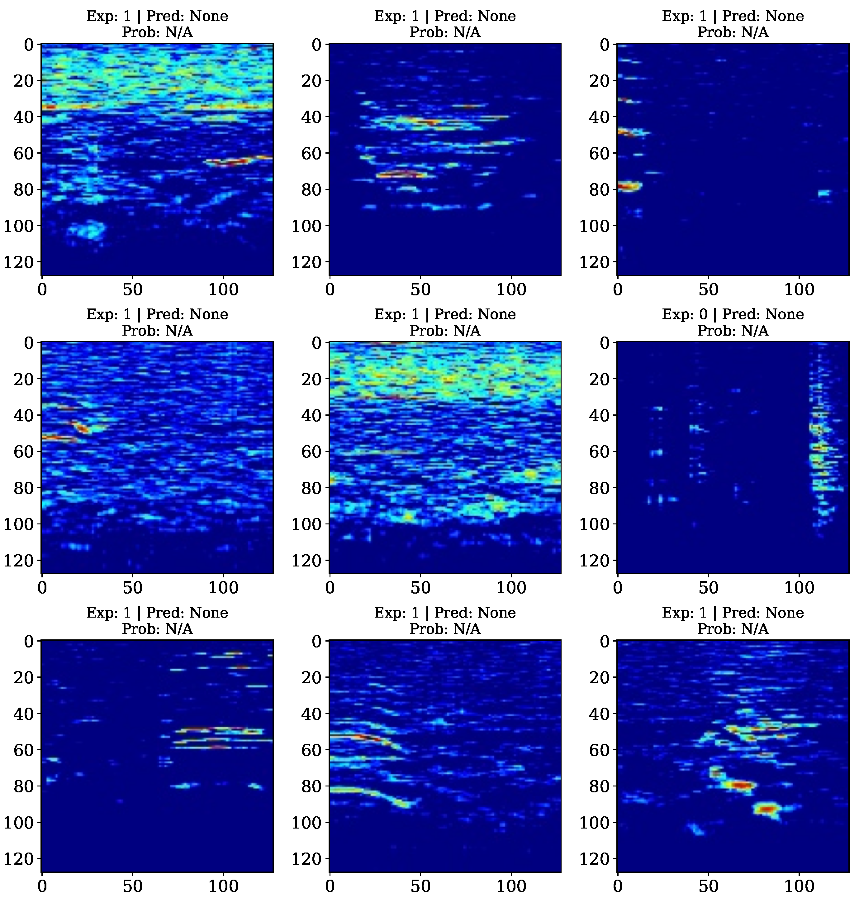
Figure 2.
Visualization of model training and validation performance metrics for the custom-built CNN architecture during supervised learning. The figure plots both (a) binary accuracy and (b) binary cross-entropy loss as functions of the training epochs.
Figure 2.
Visualization of model training and validation performance metrics for the custom-built CNN architecture during supervised learning. The figure plots both (a) binary accuracy and (b) binary cross-entropy loss as functions of the training epochs.
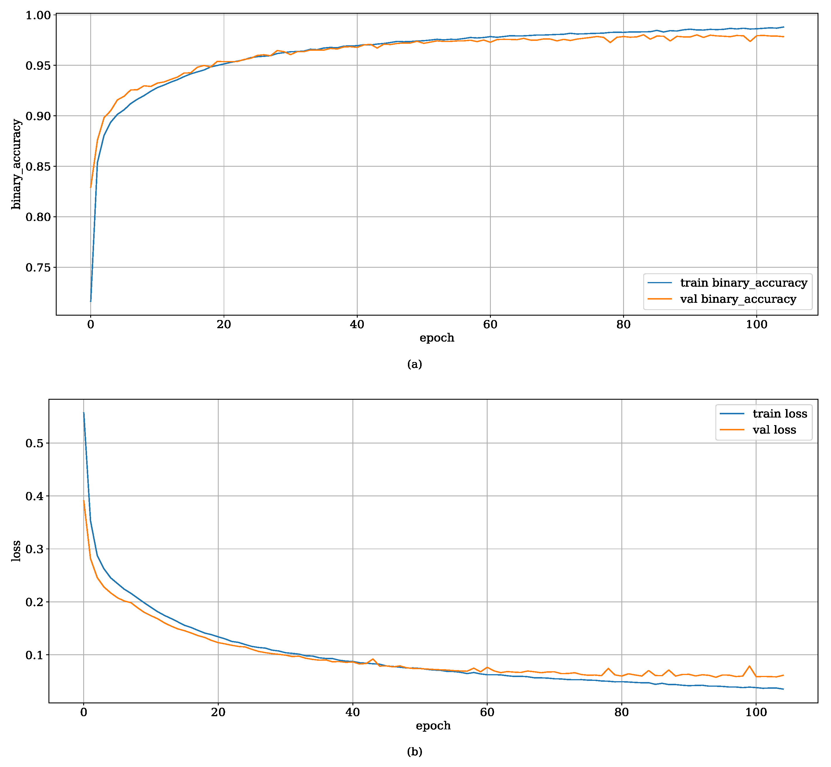
Figure 3.
Visualization of a sampled data batch from the testing set, illustrating the predictions made by the evaluated CNN model. The figure displays the input spectral images alongside their prediction probabilities and predicted class value, where green color coding indicates a correct estimation.
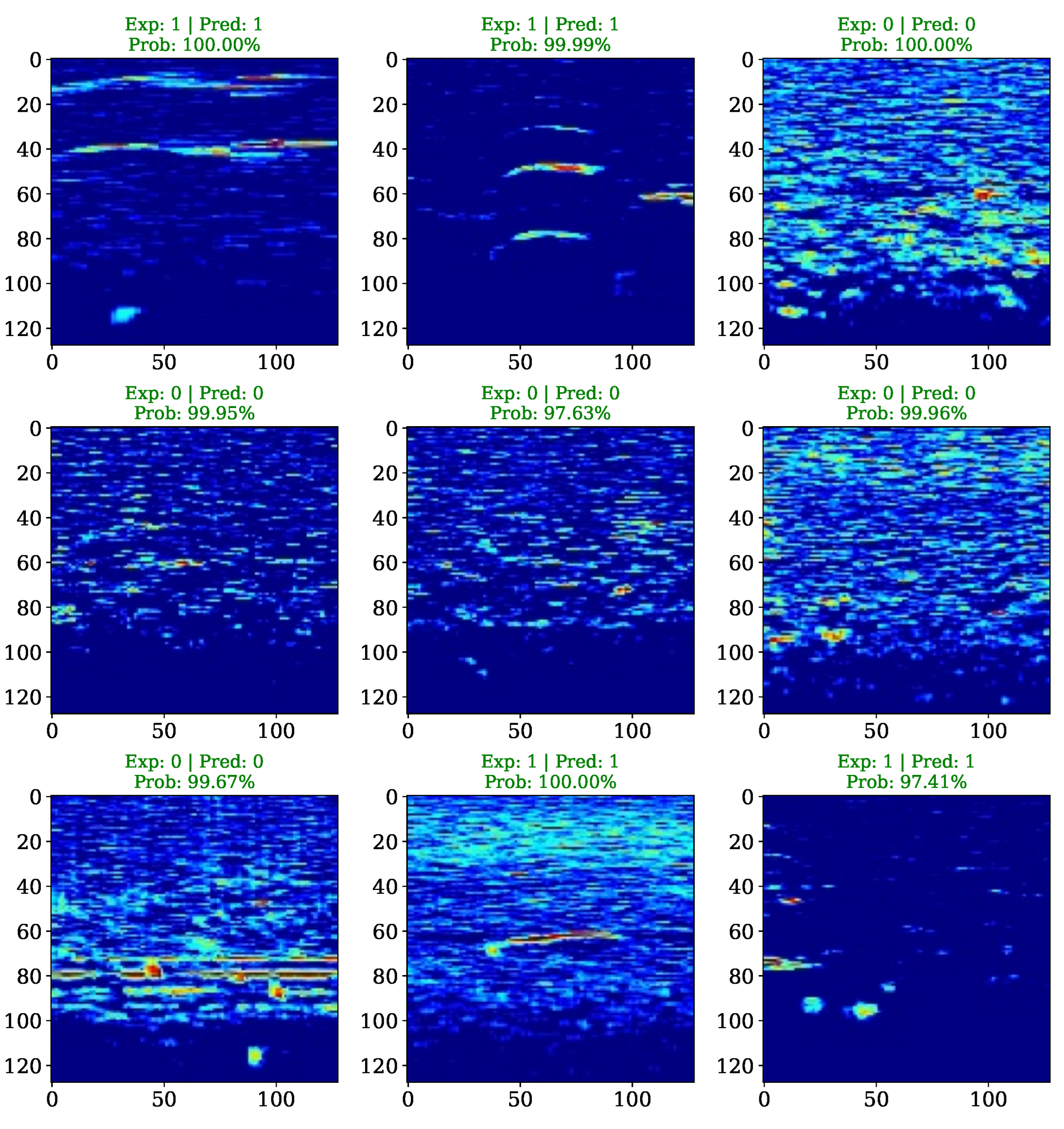
Figure 4.
Training and validation metrics during the transfer learning fine-tuning process for both pre-trained architectures. The figure plots the binary accuracy (a) and binary cross-entropy loss (b) as a function of training epochs for the VGG-16 model, alongside the corresponding binary accuracy (c) and binary cross-entropy loss (d) for the VGG-19 model.
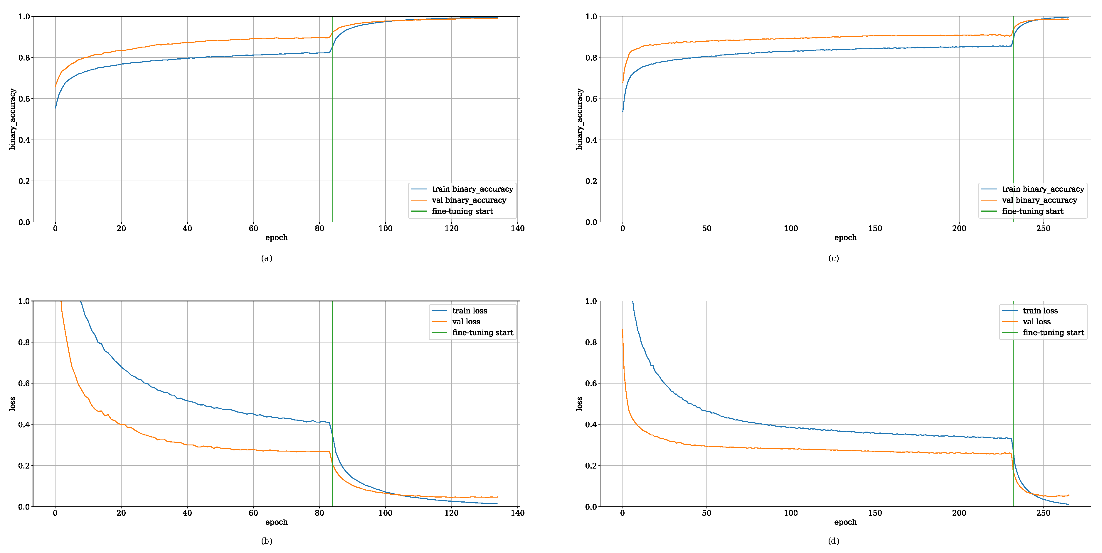
Figure 5.
Visualization of a spectrograms data batch from the testing set, displaying the predictions made by the VGG-16 model. The figure illustrates the input images alongside the calculated prediction probabilities and the final predicted class, where green color-coding indicates a correct estimation.
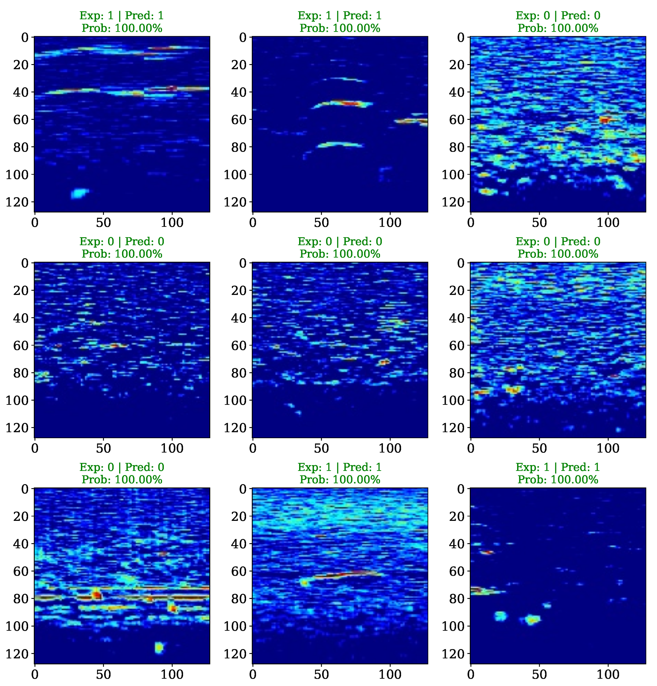
Figure 6.
Visualization of the manatee call detection inference applied to the experimental acoustic recording , illustrating the performance of the VGG-16 ensemble on unseen data. The figure presents both (a) the time domain visualization of the segment containing the detected call, annotated with the prediction confidence of belonging to a manatee call, and (b) the corresponding batch of spectral images of the inference result.
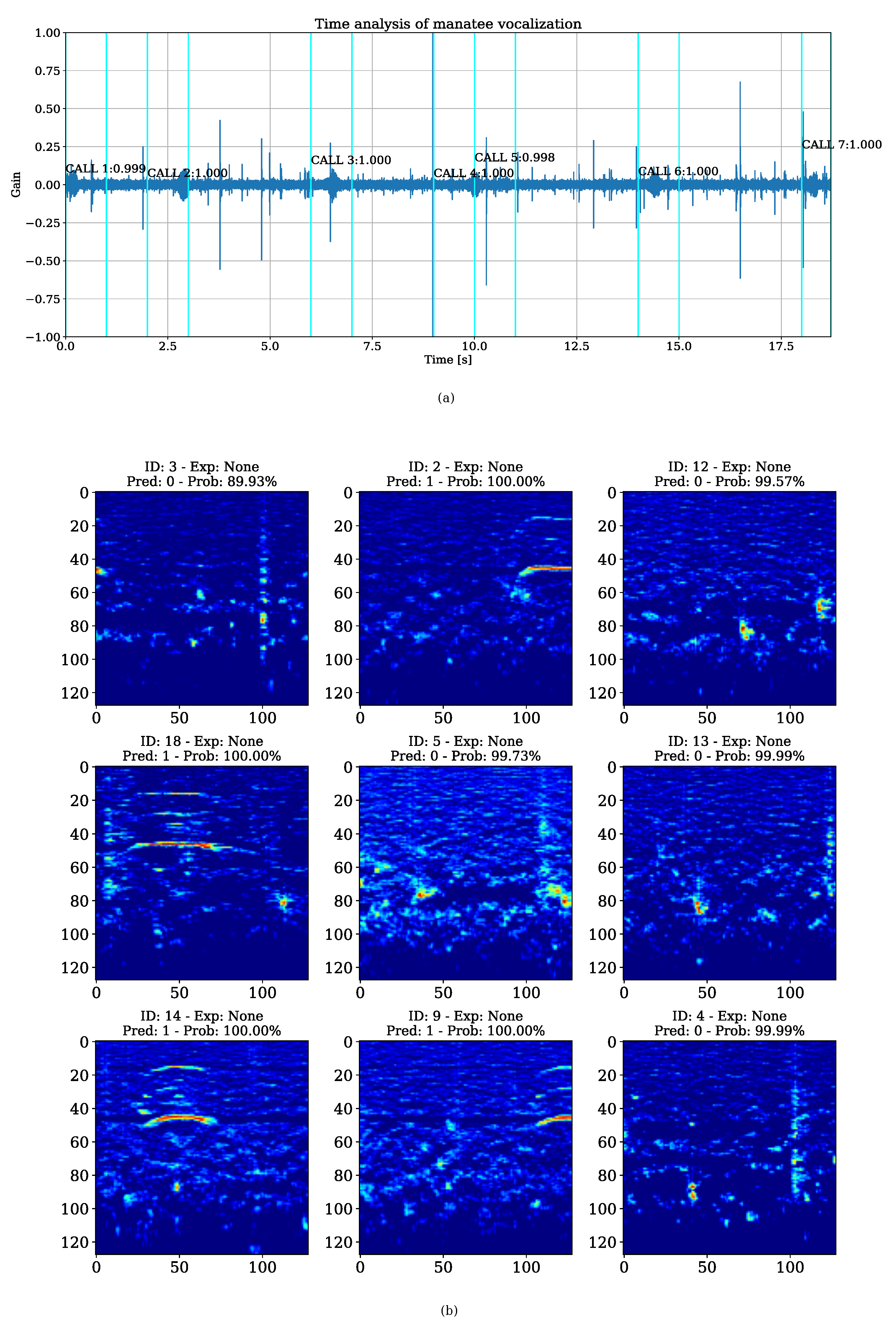
Figure 7.
Manatee population estimation via unsupervised learning. The bivariate analysis utilizes the and BW of each detected observation to group individual calls into clusters based on their MIR descriptors.
Figure 7.
Manatee population estimation via unsupervised learning. The bivariate analysis utilizes the and BW of each detected observation to group individual calls into clusters based on their MIR descriptors.
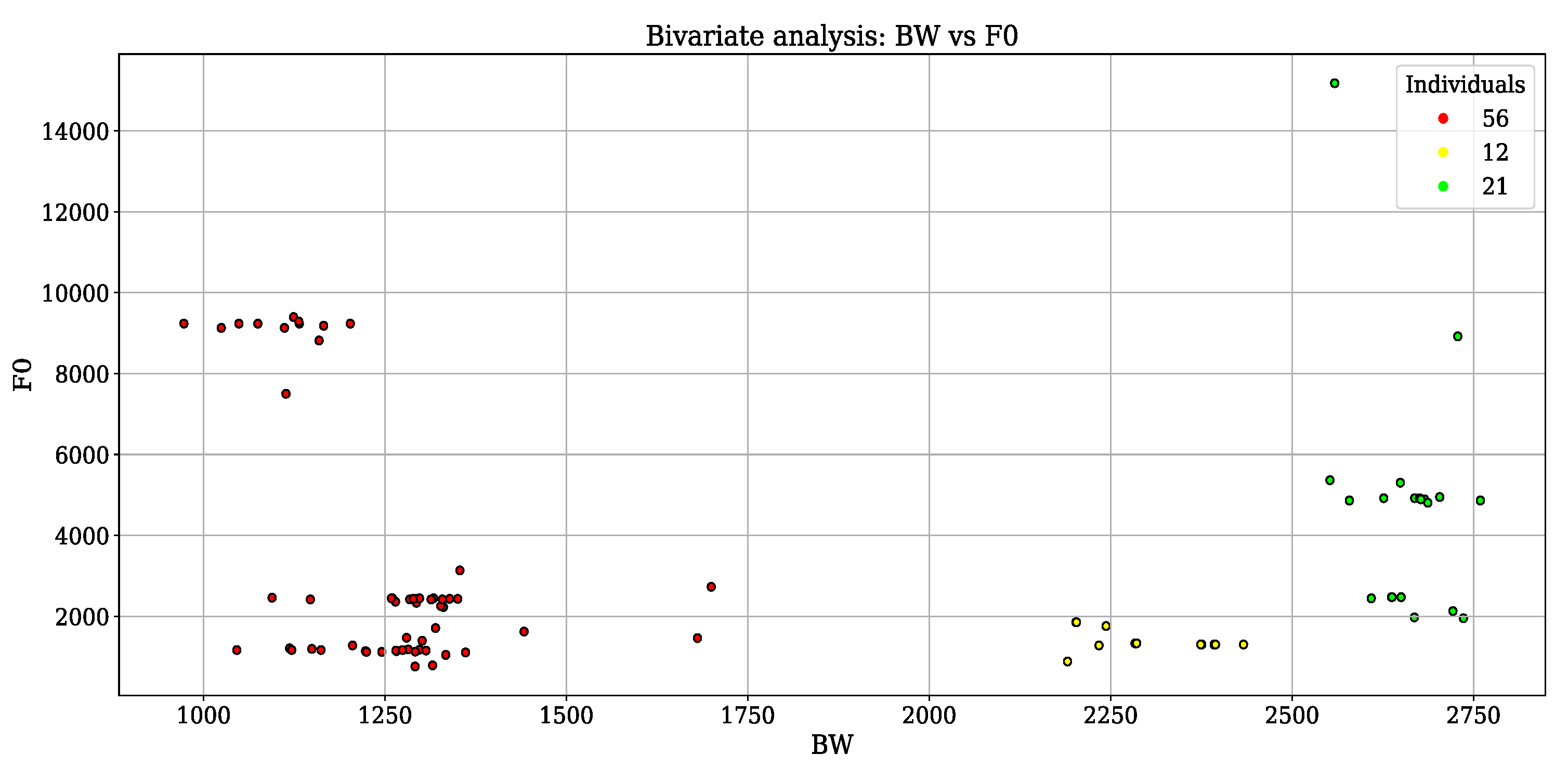

Table 1.
Hardware utilized on the Kabré supercomputer for benchmarking the operational modes of the enhanced AMCM pipeline. This implies measuring the execution time and performance of the MCD when implementing DNN architectures across both training and testing phases.
Table 1.
Hardware utilized on the Kabré supercomputer for benchmarking the operational modes of the enhanced AMCM pipeline. This implies measuring the execution time and performance of the MCD when implementing DNN architectures across both training and testing phases.
| CPUs | Memory | GPUs | OS |
|---|---|---|---|
| 2 Intel Xeon Silver 4214R CPU@2.40GHz | 31 GiB | 1 Tesla V100-PCIE-32GB | Linux 3.10.0-64bits |
| 1 Intel Xeon Silver 4416+ CPU@2.00GHz | 256 GiB | 1 NVIDIA L40S–48GB | Linux 5.14.0-64bits |
Table 2.
Confusion matrix illustrating the classification performance of the MCD model on the testing set. The matrix details the model’s ability evaluation to classify the presence and absence of manatee calls after completing the training phase of the custom-designed CNN architecture.
Table 2.
Confusion matrix illustrating the classification performance of the MCD model on the testing set. The matrix details the model’s ability evaluation to classify the presence and absence of manatee calls after completing the training phase of the custom-designed CNN architecture.
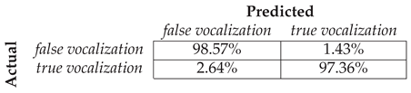 |
Table 3.
Binary classification report summarizing fundamental prediction metrics for true and false manatee calls, obtained from evaluating the MCD model based on the custom-designed CNN architecture.
Table 3.
Binary classification report summarizing fundamental prediction metrics for true and false manatee calls, obtained from evaluating the MCD model based on the custom-designed CNN architecture.
| Class | Precision | Recall | F1-score |
|---|---|---|---|
| false vocalization | 0.97 | 0.99 | 0.98 |
| true vocalization | 0.99 | 0.97 | 0.98 |
Table 4.
Confusion matrix illustrating the classification performance of the MCD model on the testing set using pre-trained large-scale weights. The results detail the model’s ability to identify the presence and absence of manatee calls following fine-tuning on the custom labeled audio database.
Table 4.
Confusion matrix illustrating the classification performance of the MCD model on the testing set using pre-trained large-scale weights. The results detail the model’s ability to identify the presence and absence of manatee calls following fine-tuning on the custom labeled audio database.
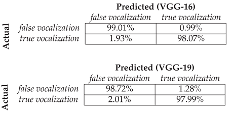 |
Table 5.
Binary classification report summarizing prediction metrics for true and false manatee calls. The results were obtained from evaluating the MCD model utilizing a transfer learning methodology, with the reported metrics being consistent for both pre-trained architectures (VGG-16 and VGG-19).
| Class | Precision | Recall | F1-score |
|---|---|---|---|
| false vocalization | 0.98 | 0.99 | 0.99 |
| true vocalization | 0.99 | 0.98 | 0.99 |
Table 6.
Quantitative results of model inference for the MCD model on unseen experimental recordings from the Panamanian Caribbean (Bocas del Toro) database [26]. Sample nomenclature is defined based on the final evaluation transcription file containing MIR attributes and individual tags.
Table 6.
Quantitative results of model inference for the MCD model on unseen experimental recordings from the Panamanian Caribbean (Bocas del Toro) database [26]. Sample nomenclature is defined based on the final evaluation transcription file containing MIR attributes and individual tags.
| Sample | Expected (n) | Predicted (n) | Valid (n) | Error |
|---|---|---|---|---|
| 4 | 5 | 4 | 0.25 | |
| 2 | 1 | 1 | 0.50 | |
| 6 | 7 | 7 | 0.17 | |
| 9 | 10 | 9 | 0.11 | |
| 4 | 7 | 7 | 0.75 | |
| 5 | 5 | 5 | 0.00 | |
| 14 | 17 | 16 | 0.21 | |
| 6 | 17 | 16 | 1.83 | |
| 16 | 21 | 21 | 0.31 | |
| 3 | 8 | 3 | 1.67 |
Disclaimer/Publisher’s Note: The statements, opinions and data contained in all publications are solely those of the individual author(s) and contributor(s) and not of MDPI and/or the editor(s). MDPI and/or the editor(s) disclaim responsibility for any injury to people or property resulting from any ideas, methods, instructions or products referred to in the content. |
© 2025 by the authors. Licensee MDPI, Basel, Switzerland. This article is an open access article distributed under the terms and conditions of the Creative Commons Attribution (CC BY) license (http://creativecommons.org/licenses/by/4.0/).
Copyright: This open access article is published under a Creative Commons CC BY 4.0 license, which permit the free download, distribution, and reuse, provided that the author and preprint are cited in any reuse.


