
Submitted:
18 December 2025
Posted:
22 December 2025
You are already at the latest version
Abstract
Antarctic ice core data reveal a consistent pattern across glacial cycles: atmospheric CO₂ does not immediately track temperature decline as interglacial conditions give way to glaciation. The most dramatic example occurs during the Last Interglacial (Eemian, MIS 5e), where CO₂ remained essentially constant at 275–280 ppm for approximately 13,000 years while temperature fell 7°C. This paper examines whether similar behavior can be detected during cooling from earlier interglacials. Using harmonic fits to temperature and CO₂ data spanning 350,000 years, phase plots are constructed of CO₂ versus temperature that isolate the warming and cooling branches of each glacial cycle. The analysis reveals that the Eemian is the clearest but not unique example: MIS 9 shows comparable behavior, while the MIS 7 complex presents an instructive exception that may reflect extreme orbital forcing conditions. The asymmetry between rapid CO₂ release during warming and slow CO₂ absorption during cooling suggests rate-limited processes govern the return of atmospheric carbon to oceanic and terrestrial reservoirs. These observations are inconsistent with CO₂ acting as the primary driver of temperature change on glacial-interglacial timescales.
Keywords:
ice core
; CO2
; interglacial
1. Introduction
Anyone who examines the Antarctic ice core data for temperature and CO₂ carefully will be forced to notice that during the Eemian (Sangamonian), Marine Isotope Stage 5e, Figure 1, shows temperature peaked and CO₂ reached its maximum for that period and then for 13,000 years CO₂ held that maximum almost constant while temperature fell 7 degrees C.
This is probably the most dramatic indication in the ice core record showing temperature falling while CO₂ holds high and constant. Can similar behavior be detected in association with other interglacials?
2. Methodology and Harmonic Fits
The analysis employs harmonic fits to Antarctic ice core proxy temperature and CO₂ data using a greedy algorithm that successively adds periodic components to minimize residual variance (Higginbotham, 2025c). Temperature data are from the EPICA Dome C deuterium-derived temperature proxy (Jouzel et al., 2007) on the EDC3 chronology (Parrenin et al., 2007). CO₂ data are from the Antarctic composite record (Bereiter et al., 2015), converted from AICC2012 to EDC3 chronology. This approach achieves R² > 0.95 for both temperature and CO₂ over the 350,000-year record. Importantly, the algorithm independently recovers the canonical Milankovitch orbital periods (approximately 100,000, 41,000, and 23,000 years; Milankovitch, 1941) without prior specification, validating both the methodology and the orbital pacing of glacial cycles.
Figure 2 displays the temperature record with harmonic fit and Marine Isotope Stage (MIS) codes. The major interglacial peaks are labeled: MIS 9 (~330,000 years ago), MIS 7e (~240,000 years ago), MIS 5e (the Eemian, ~125,000 years ago), and MIS 1 (the current Holocene). The MIS 7 complex includes several substages representing oscillations within that interglacial period.
Figure 3 shows the corresponding CO₂ record with harmonic fit. The CO₂ peaks correlate with temperature peaks but, as we will demonstrate, with systematic temporal offsets that reveal the asymmetric nature of the carbon cycle response.
3. CO₂ Versus Temperature: Evidence for Asymmetric Response
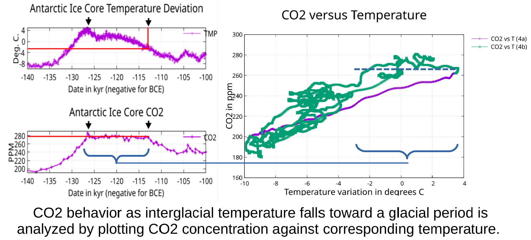
Rather than examining temperature and CO₂ as separate time series, we can plot CO₂ directly against temperature to reveal the relationship between these variables. Figure 4 presents this composite plot using the evaluation of harmonic fits from date −350,000 to 1850. The plot exhibits pronounced curvature and hysteresis, indicating that CO₂ does not respond symmetrically to warming and cooling.
If CO₂ and temperature were linearly related with a simple phase lag, the parametric plot would trace an ellipse. Instead, the observed pattern shows extended horizontal excursions during cooling phases—periods where temperature decreases substantially while CO₂ remains elevated. This is the graphical signature of the asymmetric absorption mechanism: CO₂ release during warming is relatively rapid, while CO₂ uptake during cooling is rate-limited.
4. Analysis by Interglacial Period
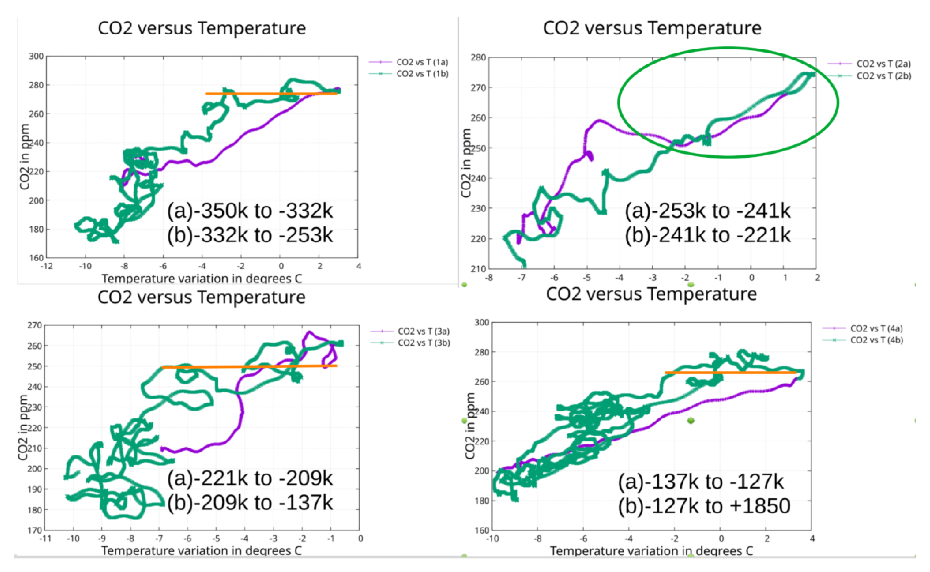
To examine whether the Eemian CO₂ plateau is unique or representative of a general pattern, Figure 5 separates the composite CO₂-temperature plot into four panels corresponding to different interglacial periods. Each panel distinguishes the warming branch (labeled 'a') from the subsequent cooling branch (labeled 'b').
4.1. MIS 9 (−350k to −253k)
The upper left panel shows MIS 9, spanning approximately −350,000 to −253,000 years. The warming phase (a) from −350k to −332k shows CO₂ rising from approximately 185 ppm to nearly 300 ppm as temperature increases from −10°C to +4°C relative to present. The cooling phase (b) from −332k to −253k exhibits the characteristic horizontal excursion: temperature begins falling while CO₂ initially holds near its peak before beginning a slower decline. This panel provides clear evidence that the delayed CO₂ response during cooling is not unique to the Eemian.
4.2. MIS 7e through MIS 7d (−253k to −221k)
The upper right panel captures MIS 7e and the subsequent MIS 7d substage. Unlike MIS 9 and MIS 5e, this panel does not show a pronounced CO₂ plateau during cooling. Instead, CO₂ appears to track temperature downward more closely as the system transitions from MIS 7e into MIS 7d.
This anomalous behavior may have a geophysical explanation worth considering. Research on speleothem records from the Austrian Alps (Moseley et al., 2021) indicates that MIS 7d coincided with the lowest Northern Hemisphere summer insolation of the past 800,000 years—387 W/m² at 65°N, caused by a rare combination of minimum obliquity and maximum precession. This extreme orbital configuration drove rapid, hemisphere-wide cooling: atmospheric CO₂ fell below 203 ppm, North Atlantic sea surface temperatures dropped to near-glacial levels, and European pollen records indicate glacial-like conditions.
4.3. MIS 7c Through MIS 6 (−221k to −137k)
The lower left panel spans the later substages of MIS 7 and the transition into MIS 6 (the Saalian glaciation). This period follows the anomalous MIS 7d interval and shows more complex behavior.
Interestingly, the cooling branch (b) from −209k to −137k does appear to show horizontal excursions where CO₂ holds relatively constant while temperature declines—but at a cooler baseline than observed in MIS 9 or MIS 5e. The entire pattern is shifted to temperatures around −1°C to −7°C and CO₂ levels in the 230–260 ppm range.
One possible interpretation is that after the extreme MIS 7d cooling event ended, the carbon cycle resumed its normal asymmetric behavior, but operating within the cooler, lower-CO₂ regime characteristic of MIS 7. The "failed interglacial" nature of MIS 7—which never achieved the warmth of MIS 5e or MIS 9 — may have compressed the entire CO₂-temperature relationship into a narrower range while preserving the underlying asymmetric dynamics.
This interpretation remains conjectural. The complexity of the MIS 7 substage oscillations makes it difficult to isolate clean warming and cooling branches comparable to those in MIS 9 and MIS 5e.
4.4. MIS 5e Through MIS 1 (−137k to +1850)
The lower right panel presents the most recent and best-resolved portion of the record, including the Eemian (MIS 5e) and the current Holocene (MIS 1). The warming phase (a) from −137k to −127k shows the sharp rise into the Eemian peak, with CO₂ and temperature rising together along a steep trajectory.
The subsequent cooling branch (b) from −127k to −110k displays the most dramatic example of the phenomenon under investigation. Temperature falls approximately 7°C (from +4°C to −3°C) while CO₂ barely changes from its peak near 280 ppm. This is the 13,000-year Eemian plateau—the most striking demonstration in the ice core record that CO₂ does not immediately follow temperature during glacial cooling.
The clarity of this signal likely reflects both the magnitude of the Eemian warmth (creating a large CO₂ "excess" requiring reabsorption) and the superior temporal resolution of the more recent ice core data. The Eemian thus serves as the type example of asymmetric carbon cycle response, with MIS 9 providing independent confirmation that this behavior is a recurring feature of glacial cycles.
5. Discussion
The analysis reveals that the Eemian CO₂ plateau, while the most dramatic example, represents an extreme case of a general pattern observable across multiple glacial cycles. In each transition from interglacial warmth to glacial cold, CO₂ shows a delayed response, remaining elevated while temperature has already begun its decline. The exception during MIS 7d, if correctly interpreted as a consequence of extreme orbital forcing, actually reinforces the underlying mechanism by demonstrating that sufficiently rapid cooling can overcome the rate limitation.
5.1. Mechanisms for Asymmetric Response
Several mechanisms may contribute to the observed asymmetry between CO₂ release and absorption:
Atmospheric transport limitation: When the ocean warms, dissolved CO₂ is immediately available at the air-sea interface for release. When the ocean cools, CO₂ that was released during warming is dispersed throughout the atmosphere and must find its way back to the ocean surface through atmospheric mixing—a rate-limited process.
Sea ice expansion: Growing sea ice during cooling physically caps the ocean surface, reducing the area available for gas exchange for the coldest ocean. The Southern Ocean and North Atlantic, major regions of deep water formation and CO₂ exchange, become progressively ice-covered during glacial descent.
Plant stress feedback: As CO₂ begins to decline during cooling, vegetation—particularly C3 plants that comprise most forests—experiences carbon limitation. This stress reduces photosynthetic uptake and may cause vegetation die-off, releasing stored carbon and creating a negative feedback that resists CO₂ decline.
5.2. Implications for Causality
The consistent observation of temperature declining while CO₂ remains constant poses a challenge for hypotheses in which CO₂ is the primary driver of temperature change. If CO₂ were driving temperature, a 7°C temperature decline while CO₂ remained constant would require invoking other forcings of comparable magnitude operating in the opposite direction to CO₂—forcings that would need to precisely cancel the expected warming effect of elevated CO₂ for 13,000 years.
The more parsimonious interpretation is that temperature, driven primarily by orbital (Milankovitch) forcing, leads the system, with CO₂ responding as a feedback through ocean degassing, circulation changes, and biosphere responses (Humlum et al., 2013; Grabyan, 2025). The asymmetric response times—fast release, slow uptake—create the observed plateaus during the cooling phases of glacial cycles. Climate models continue to have difficulty reproducing glacial inception (Vavrus et al., 2018; Willeit et al., 2024), suggesting that current understanding of the feedback mechanisms governing interglacial-to-glacial transitions remains incomplete.
6. Conclusions
- The Eemian CO₂ plateau—13,000 years of constant CO₂ while temperature fell 7°C—is the most dramatic but not unique example of delayed CO₂ response during glacial cooling.
- Phase plots of CO₂ versus temperature reveal systematic asymmetry: rapid CO₂ rise during warming, delayed CO₂ decline during cooling.
- MIS 9 shows comparable behavior to MIS 5e, confirming this is a recurring feature of glacial cycles spanning at least 350,000 years.
- The MIS 7d interval may represent an instructive exception: extreme orbital forcing (the lowest NH summer insolation in 800,000 years) potentially overwhelmed the rate-limiting mechanisms, allowing CO₂ to track temperature downward.
- The pattern is consistent with rate-limited processes governing CO₂ absorption: atmospheric transport, sea ice formation, and plant stress feedbacks.
- These observations support the interpretation that orbital forcing drives temperature, with CO₂ acting as a delayed feedback rather than the primary driver of glacial-interglacial temperature variations.
Funding
This research received no external funding.
Acknowledgments
I would like to thank Renee Hannon for directing my interest toward this subject.
Conflicts of Interest
The author declares no conflicts of interest.
References
- Bereiter, B.; Eggleston, S.; Schmitt, J.; Nehrbass-Ahles, C.; Stocker, T.F.; Fischer, H.; Kipfstuhl, S.; Chappellaz, J. Revision of the EPICA Dome C CO₂ record from 800 to 600 kyr before present. Geophysical Research Letters 2015, 42, 542–549. [Google Scholar] [CrossRef]
- Grabyan, R. Global Atmospheric CO₂ Lags Temperature: Implications for Short- and Long-Term Climate Predictions. Science of Climate Change 2025, 5(3), 302–326. [Google Scholar]
- Higginbotham, J. Planetary Orbits and Sea-Level During the Phanerozoic: Correlation, Causation, and Forecasting. Journal of Biomedical Research & Environmental Sciences 2025a, 6(4), 926–940. [Google Scholar]
- Higginbotham, J. Climate, Water Vapor, and Volcanic Eruptions. Preprints.org 2025b. [Google Scholar] [CrossRef]
- Higginbotham, J. Antarctic Ice Core Harmonic Analysis. Preprints.org 2025c. [Google Scholar] [CrossRef]
- Humlum, O.; Stordahl, K.; Solheim, J.E. The phase relation between atmospheric carbon dioxide and global temperature. Global and Planetary Change 2013, 100, 51–69. [Google Scholar] [CrossRef]
- Jouzel, J.; et al. Orbital and Millennial Antarctic Climate Variability over the Past 800,000 Years. Science 2007, 317(5839), 793–796. [Google Scholar] [CrossRef] [PubMed]
- Milankovitch, M. Kanon der Erdbestrahlung und seine Anwendung auf das Eiszeitenproblem; Royal Serbian Academy Special Publication 133: Belgrade, 1941. [Google Scholar]
- Moseley, G.E.; et al. Precise timing of MIS 7 substages from the Austrian Alps. Climate of the Past 2021, 17, 1443–1454. [Google Scholar] [CrossRef]
- Parrenin, F.; Barnola, J.-M.; Beer, J.; Blunier, T.; Castellano, E.; Chappellaz, J.; Dreyfus, G.; Fischer, H.; Fujita, S.; Jouzel, J.; Kawamura, K.; Lemieux-Dudon, B.; Loulergue, L.; Masson-Delmotte, V.; Narcisi, B.; Petit, J.-R.; Raisbeck, G.; Raynaud, D.; Ruth, U.; Schwander, J.; Severi, M.; Spahni, R.; Steffensen, J.P.; Svensson, A.; Udisti, R.; Waelbroeck, C.; Wolff, E. The EDC3 chronology for the EPICA Dome C ice core. Climate of the Past 2007, 3, 485–497. [Google Scholar] [CrossRef]
- Vavrus, S.J.; He, F.; Kutzbach, J.E.; Ruddiman, W.F.; Tzedakis, P.C. Glacial Inception in Marine Isotope Stage 19: An Orbital Analog for a Natural Holocene Climate. Scientific Reports 2018, 8, 10213. [Google Scholar] [CrossRef] [PubMed]
- Willeit, M.; Calov, R.; Talento, S.; Greve, R.; Bernales, J.; Klemann, V.; Bagge, M.; Ganopolski, A. Glacial inception through rapid ice area increase driven by albedo and vegetation feedbacks. Climate of the Past 2024, 20, 597–623. [Google Scholar] [CrossRef]
Figure 1.
Here CO2 is seen to hold constant for 13,000 years while temperature falls 7 degrees C. Figure taken from Higginbotham 2025b.
Figure 1.
Here CO2 is seen to hold constant for 13,000 years while temperature falls 7 degrees C. Figure taken from Higginbotham 2025b.
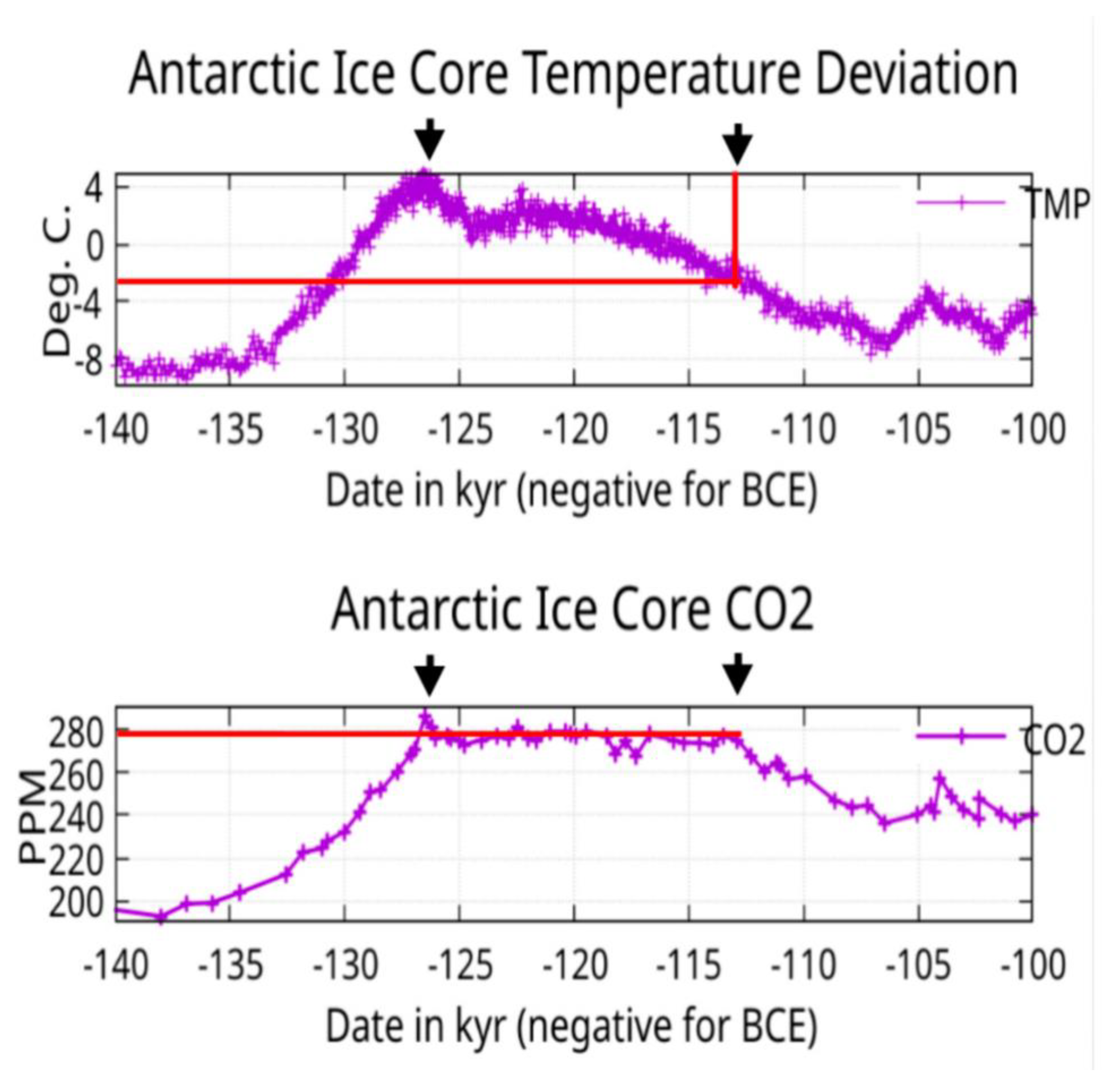
Figure 2.
Temperature record from date -350,000 to 1911 with negative dates indicating BCE. Figure taken from Higginbotham 2025b. Marine Isotope Stage (MIS) codes added.
Figure 2.
Temperature record from date -350,000 to 1911 with negative dates indicating BCE. Figure taken from Higginbotham 2025b. Marine Isotope Stage (MIS) codes added.
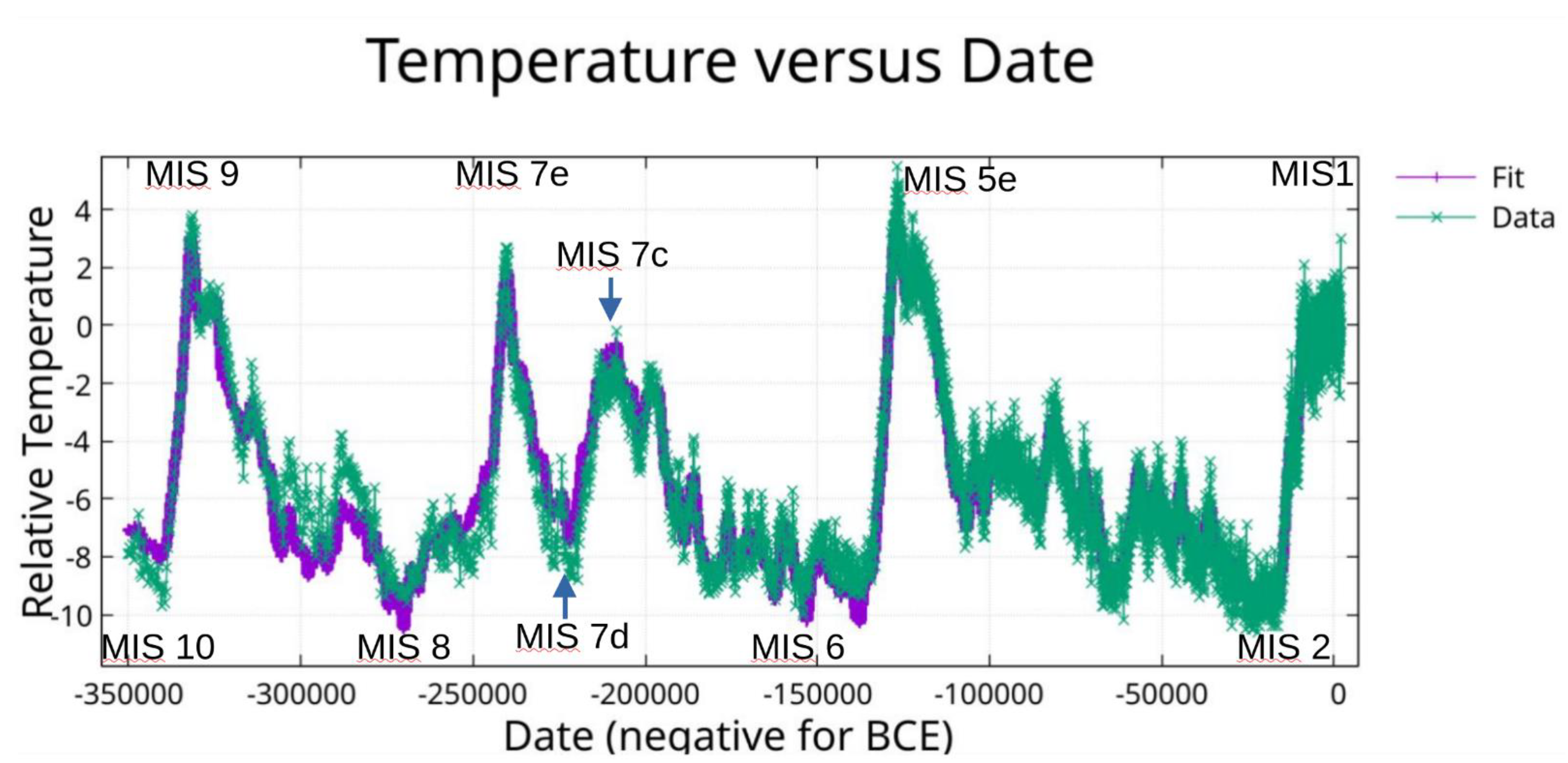
Figure 3.
Atmospheric CO₂ record from date -350,000 to 1911 with negative dates indicating BCE. Figure taken from Higginbotham 2025b.
Figure 3.
Atmospheric CO₂ record from date -350,000 to 1911 with negative dates indicating BCE. Figure taken from Higginbotham 2025b.
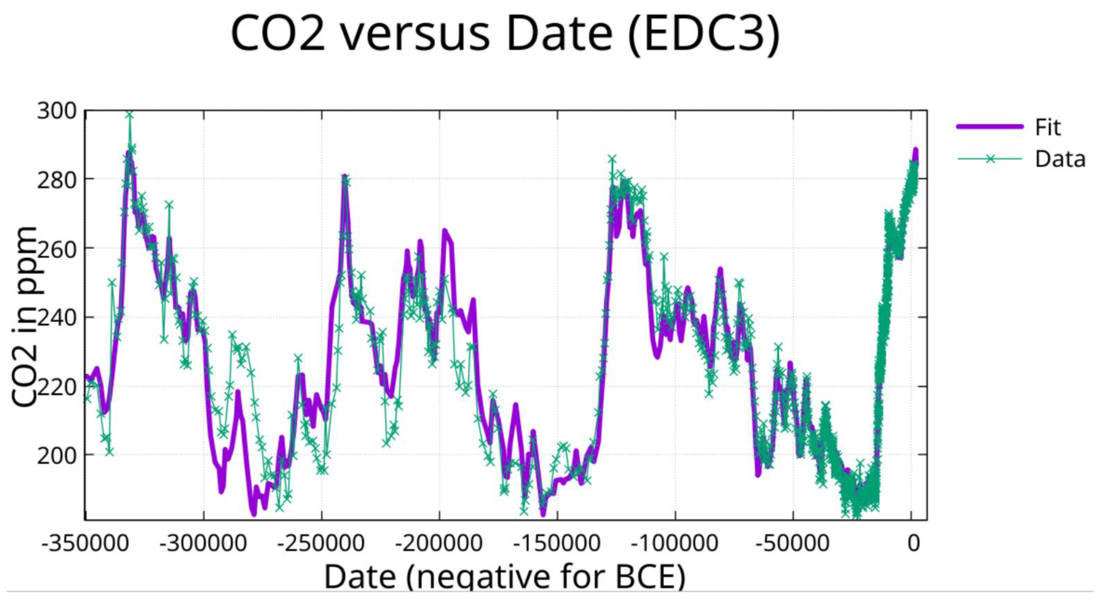
Figure 4.
Plot of CO2 versus temperature from Higginbotham 2025b. This plot is a composite of the evaluation of the fits to CO2 and Temperature from date -350,000 to 1850. This plot shows a curvature in the composite plot.
Figure 4.
Plot of CO2 versus temperature from Higginbotham 2025b. This plot is a composite of the evaluation of the fits to CO2 and Temperature from date -350,000 to 1850. This plot shows a curvature in the composite plot.
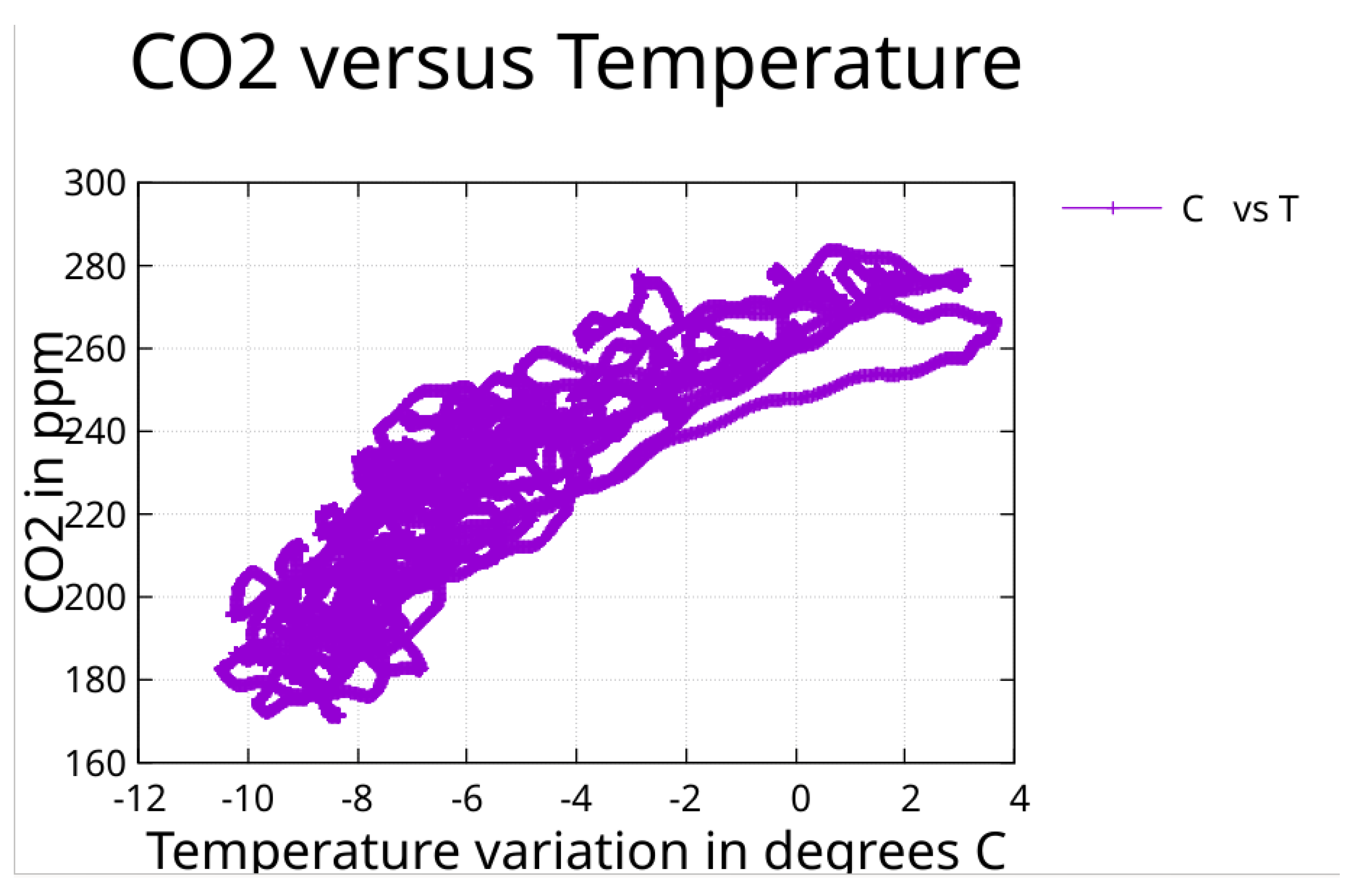
Figure 5.
Here the plot from the previous figure is split into four separate plots.Upper left shows the MIS 9 rise in temperature (a) and subsequent fall in temperature (b). Upper right shows the MIS 7e rise in temperature (a) followed by fall in temperature through MIS 7d (b). Lower left shows MIS 7c through MIS 6 with rising temperature (a) and falling and rising temperature (b). Lower right shows MIS 5e through MIS 1 with rising temperature of MIS 5e (a) and falling and rising temperature following (b).
Disclaimer/Publisher’s Note: The statements, opinions and data contained in all publications are solely those of the individual author(s) and contributor(s) and not of MDPI and/or the editor(s). MDPI and/or the editor(s) disclaim responsibility for any injury to people or property resulting from any ideas, methods, instructions or products referred to in the content. |
© 2025 by the authors. Licensee MDPI, Basel, Switzerland. This article is an open access article distributed under the terms and conditions of the Creative Commons Attribution (CC BY) license (http://creativecommons.org/licenses/by/4.0/).
Copyright: This open access article is published under a Creative Commons CC BY 4.0 license, which permit the free download, distribution, and reuse, provided that the author and preprint are cited in any reuse.


