
Submitted:
16 December 2025
Posted:
18 December 2025
You are already at the latest version
Abstract
We present a supervised method to estimate two local descriptors of time-series dynamics, the mean-reversion rate θ and a heavy tail estimate α, from short windows of data. These parameters summarize recovery behavior and tail heaviness and are useful for interpreting stochastic signals in sensing applications. The method is trained on synthetic, dimensionless Ornstein–Uhlenbeck processes with α-stable noise, ensuring robustness for non-Gaussian and heavy-tailed inputs. Gradient-boosted tree models (CatBoost) map window-level statistical features to discrete (α, θ) categories with high accuracy and predominantly adjacent-class confusion. Using the same trained models, we analyze daily financial returns, daily sunspot numbers, and NASA POWER climate fields for Austria. The method detects changes in local dynamics, including shifts in financial tail structure after 2010, weaker and more irregular solar cycles after 2005, and a redistribution in clear-sky shortwave irradiance around 2000. Because it relies only on short windows and requires no domain-specific tuning, the framework provides a compact diagnostic tool for signal processing, supporting characterization of local variability, detection of regime changes, and decision making in settings where long-term stationarity is not guaranteed.
Keywords:
Ornstein–Uhlenbeck
; Lévy
; Gaussian
; mean reversion
; complexity metrics
; machine learning
1. Introduction
Mean reversion and heavy tails are two recurring features of real-world time series. The Ornstein–Uhlenbeck (OU) process captures mean reversion through a linear drift toward equilibrium [1]. In its Gaussian form, increments are light-tailed, and the second-order structure fully characterizes variability. Many applications, however, show departures from Gaussianity: returns in finance, intermittency in environmental series, and burst-like activity in solar and geophysical records. A tractable extension replaces Brownian motion by a symmetric -stable Lévy driver with stability index , which preserves mean reversion while allowing heavy tails and occasional large jumps [2,3]. When , the variance is infinite, so methods relying on low-order moments can become unstable or biased.
Jointly estimating a mean-reversion rate and a tail index from finite, noisy data is difficult. Likelihood-based inference for stable-driven OU models requires either long samples or numerical inversion of characteristic functions and careful treatment of normalization; performance deteriorates as moves away from the Gaussian boundary [4]. Moment and cumulant approaches are not well-defined when moments diverge. Tail-quantile and peak-over-threshold methods focus on extremes but ignore the temporal structure that informs the mean reversion rate . These gaps motivate an approach that uses short-window information beyond low-order moments that scales to diverse types of data/signals.
Why is this important? Many operational decisions depend on distinguishing transient noise from persistent regime changes. In finance, separating Gaussian from heavy-tailed periods and identifying changes in reversion speed affects risk limits, hedging, and stress testing [5,6,7,8,9,10]. [8] provide an early and systematic analysis of mean reversion in financial time series based on variance-ratio methods. Their results demonstrate that deviations from a random-walk benchmark can be detected in short windows and that mean-reverting dynamics appear intermittently across asset classes. This aligns with our objective of classifying local windows by reversion strength rather than assuming stable long-run parameters. Relatedly, [11] show a structural increase in complexity and a persistent decline in out-of-sample predictability for major equity indices. They show that increases in approximate and sample entropy correspond to weaker forecasting performance of a wide range of ML models. This supports our motivation to jointly screen windows for Gaussian vs. non-Gaussian features and for strong vs. weak reversion, since both characteristics are linked to shifts in local predictability and model stability. In environmental monitoring, heavy-tailed windows and weak short-horizon reversion indicate intermittent events and regime persistence, which influence planning and early warning [12,13,14]. In scientific data analysis, reliable identification of heavy tails and mean reversion supports model selection and hypothesis testing when moments are undefined or uninformative [2,15]. A window-based classifier that does not rely on strong distributional assumptions enables rolling-window-based analysis, cross-domain comparability, and robust summaries in settings where classical estimators fail, are expensive to deploy, or require long observation horizons, especially for live data stream analysis [16,17,18].
We address this by developing a supervised learning approach that maps window-level features to discrete classes for . Each sample is a fixed-length segment of a dimensionless OU process; a vector of numeric descriptors summarizes ordinal patterns and short-horizon dynamics without assuming finite variance (e.g., permutation-based features [18]). We use CatBoost, a gradient-boosted decision-tree method designed for tabular inputs [19,20]. CatBoost’s ordered boosting and oblivious-tree structure provide stable and fast training and work well with categorical, as well as in our case, purely numeric features.
The synthetic-data, i.e. the employed Ornstein Uhlenbeck processes establish the ground truth and control the task’s granularity. We generate dimensionless OU series on a grid of and using exact discrete transitions for both Gaussian and stable drivers. Base series have fixed length and are segmented into overlapping windows of sizes with shift . For every w, we compute the same feature set, train two independent CatBoost classifiers (one for , one for ), and evaluate on independent-seed test sets that share the parameter grids but not the noise realizations. We report per-class precision, recall, and score, overall accuracy, and weighted score, along with absolute and row-normalized confusion matrices. This approach quantifies (i) separability as a function of window length and (ii) where misclassifications occur in parameter space. To reflect a frequent screening use case, we also evaluate the same trained models on binary classifications as well, i.e., Gaussian vs. non-Gaussian () and mean reversion v.s. no mean reversion ()—without retraining. Finally we test, evaluate and interpret our approach on several real-life time series. Figure 1 depicts the main idea.
A central objective of this work is to demonstrate that short-window statistical diagnostics can recover meaningful regime information across real-world systems. We therefore analyze heterogeneous datasets—daily financial returns, daily sunspot numbers, and environmental measurements—not because they share a physical mechanism, but because they offer complementary testbeds with well-documented regime structure. First, these domains exhibit transitions between markedly different dynamical states (e.g., volatility shifts in financial markets, solar-cycle phases in sunspot activity), making them suitable for evaluating whether short-window classifiers can detect changes that traditionally require long-term aggregation [6,21]. Second, each dataset provides a distinct stress case for robustness: financial returns contain heavy tails and clustered volatility, sunspot numbers have quasi-periodic but irregular cycles, and NASPAW data include meteorological noise and intermittent extremes. Demonstrating consistent performance across such systems highlights that the proposed framework functions as a general-purpose analysis tool.
More broadly, the models introduced here should be understood as methodological tools rather than domain-specific predictors. Many classical approaches to estimating distributional properties or mean-reversion rates rely on long samples and strong parametric assumptions; this limits their usefulness when regime changes occur on short horizons or when assumptions (such as finite variance) do not hold. The presented machine-learning approach, by contrast, enables data-driven detection of local dynamical structure from relatively small windows, offering a scalable approach for identifying short-term regime changes in settings where traditional estimators fail or require prohibitively long data records.
This paper makes four contributions. First, it provides an exact, dimensionless simulation of stable-driven OU paths across a wide grid for supervised learning. Second, it shows that window-level features paired with boosted tree models recover both tail index and reversion rate with useful fidelity, with errors concentrated between neighboring classes and accuracy improving with window length. Third, it documents a compact binary screening mode that reuses the same models to flag Gaussian vs. non-Gaussian regimes and the presence vs. absence of short-horizon mean reversion. Fourth, it applies the method to financial, environmental, and solar time series to illustrate how regime mixes shift across assets, variables, and time intervals.
The remainder of the paper is organized as follows. Section 3 introduces the Ornstein–Uhlenbeck model with -stable increments, the exact discretization used for generating synthetic benchmarks, and the window-level feature set. Section 4 specifies the supervised learning setup, including the CatBoost classifiers, the windowing procedure, data splits, and the training protocol. Section 5 outlines the validation framework and reports the full multi-class results on synthetic data together with the corresponding confusion matrices; the complementary binary evaluations are provided in Appendix A. Section 6, Section 7 and Section 8 present the empirical applications to financial returns, daily sunspot numbers, and NASA POWER climate variables for Austria, illustrating how the method identifies short-window regime changes across heterogeneous real-world signals. Section 9 summarizes the main findings and discusses limitations and practical use cases. Section 10 conlcudes this article.
2. Related Work
A growing line of research connects time–series complexity with the achievable accuracy of machine and deep learning predictors. Survey evidence shows that entropy- and fractal-based descriptors (e.g., Hurst exponent, fractal dimension, Lyapunov spectrum) help quantify persistence, intermittency, and predictability, and that models which account for these properties tend to perform better on difficult, noisy signals [22]. Building on this, several studies operationalize the link by filtering or shaping model outputs according to signal complexity: ensemble LSTMs combined with complexity filters reduce error and limit overfitting without expensive hyperparameter tuning [23]; reconstructed phase spaces and phase-space–consistent filtering stabilize autoregressive neural forecasts across datasets [24]; and stochastic interpolation that preserves attractor geometry (via fractional Brownian bridges) improves data density while maintaining dynamical structure [25]. Complementary work shows that complexity-aware interpolation—especially when guided by fractal metrics—can lift LSTM performance on short or coarse data and better handle long-memory behavior [26].
Our contribution follows this arc but targets the interpretable regime classification that is useful beyond prediction alone. Instead of using complexity solely as auxiliary features, we estimate two window-local, physically meaningful quantities: tail heaviness () and mean-reversion speed (). Trained on OU processes with -stable increments, the resulting classifiers act as compact “regime sensors” that travel across domains. We validate them on synthetic data and then apply them to three heterogeneous real datasets (finance, sunspots, and environmental series), showing that the same complexity-informed framing supports both predictive tasks (where prior work emphasized LSTM ensembles and interpolation [23,24,25,26,27]) and diagnostic tasks (where our labels summarize distributional shape and recovery dynamics). In short, this extends the complexity–predictability link surveyed by Raubitzek and Neubauer [22] into a regime-mapping tool that is practical for out-of-sample monitoring in real systems.
3. Ornstein–Uhlenbeck Processes
The Ornstein–Uhlenbeck (OU) process was introduced by Uhlenbeck and Ornstein to model velocity relaxation in a gas [1]. It is now a standard mean-reverting stochastic differential equation (SDE) with broad use in physics, finance, and engineering [28,29,30]. In its basic form the process satisfies
where t denotes time, is the mean-reversion rate towards the level , is the diffusion (noise) scale, and is a standard Brownian motion. We write for the normal distribution with mean m and variance v.
Equation (1) admits the explicit solution obtained by variation of constants,
where is the initial value at . Conditioned on , the process is Gaussian with
As , the conditional mean converges to and the conditional variance converges to , hence
If the process is initialized from the stationary distribution (or after transients are negligible), the stationary autocovariance is
so the characteristic relaxation time is . This relaxation time quantifies the temporal scale over which correlations decay and the process loses memory of past states. Specifically, after a time interval of order , the autocovariance has decreased by a factor of , indicating that deviations from the mean level are largely dissipated. Larger values of therefore correspond to faster mean reversion and shorter memory, while smaller values of imply slower relaxation and more persistent temporal dependence.
Over a fixed sampling interval , the transition density is Gaussian. Sampling at times and writing gives the exact recursion
Equivalently, the conditional distribution is
This is the closed-form (non-Euler–Maruyama) update; therefore no additional factor multiplies .
For parameter inference it is convenient to remove location and scale while preserving mean reversion. Define the dimensionless, centered, and scaled process
Since , Equation (8), is affine in , Itô’s formula reduces to differentiation of the map with and :
Hence, in the stationary regime, has mean 0 and variance 1. The exact discrete transition, Equation (9), over is
Equation (9) keeps as the single free parameter in the Gaussian OU case.
3.1. Replacing the Wiener Driver by Symmetric -Stable Noise
Empirical series in several domains exhibit heavy tails and jumps that occur more often than Gaussian models predict. A natural extension replaces in (9) by the increment of a symmetric () -stable Lévy process .
A random variable X is stable if sums of i.i.d. copies are equal in law to a location–scale transform of X. We write with stability , skewness , scale , and location . For , the characteristic function is
For the characteristic function has a different (logarithmic) form; in this work we use the symmetric case , for which the characteristic function reduces to . Special cases: gives ; with and one obtains the Cauchy law. Moments satisfy iff .
Let be a symmetric -stable Lévy motion with independent, stationary increments and
i.e., the increment scale grows like (unit scale at ).
We consider the Lévy-driven OU SDE
The solution admits the moving-average representation
In the stationary regime (or for ), the marginal distribution of is again -stable [31]. To determine its scale, use the stability property of stochastic integrals with respect to : for deterministic ,
With , we obtain the stationary scale parameter
To keep the dimensionless convention (unit stationary scale for all ), we choose
which yields and hence the stationary marginal for every .
Let and . From (13),
By stationarity and independence of Lévy increments, the integral term is independent of and has the same law as . Using the scaling rule for stable integrals,
where . Therefore the exact transition can be written as
Evaluating the integral gives , so with the normalization (15) this simplifies to
For , corresponds to a Gaussian draw and (18) reduces to the Gaussian transition (10).
In the implementation, we draw using scipy.stats.levy_stable, which follows Nolan’s parameterization. At , , and scale, this sampler returns rather than . Therefore, when we rescale the draw by to match in (10). Alternatively, one may bypass the stable sampler at and draw Z directly.
- exponential pull toward zero; larger implies faster mean reversion.
- tail index; smaller yields heavier tails and larger jumps; is Gaussian.
- noise scale in (12); with the stationary marginal scale is 1 for all .
3.2. Simulation Setup and Implementation
We use symmetric -stable noise () with , spanning the range from Gaussian () to extremely heavy-tailed regimes (small ).
Stable variates are generated with
which returns i.i.d. draws from . Inserting these into (18) yields the exact one-step update used for simulation. At , scale corresponds to (i.e., norm with scale), so we rescale by to obtain [32].
To generate time series for supervised learning, we discretize the dimensionless OU model on a uniform grid.
We use the exact transition (10):
For we use the exact transition (18):
This choice is consistent with the SDE normalization and keeps the stationary marginal scale equal to one for all .
The resulting dimensionless series provide a homogeneous input space across for feature extraction and learning.
These dimensionless Ornstein–Uhlenbeck processes are depicted in Figure 2 and Figure 3 for several parameter combinations .
Stability index.
We explore the five values
each with skewness fixed at (symmetric law). The choice spans the full range from the Gaussian case () to an extreme heavy-tail regime (). For reference:
- (1)
- : normal distribution; finite mean and variance.
- (2)
- : infinite variance but finite mean; moderate tails.
- (3)
- : Cauchy-type; mean and variance both infinite.
- (4)
- : very heavy tails; large jumps common.
- (5)
- : extreme heavy-tail regime with rare but dominating outliers.
Mean-reversion rate.
A separate grid
with , controls how fast the process returns to equilibrium. Concrete values are specified in Section 5.
Noise scale.
We keep the stationary marginal scale equal to one by setting
see equation (15). This normalization allows direct comparison of paths across different .
Stable increments are generated with scipy.stats.levy_stable.rvs [32,33]. The call returns i.i.d. variables that feed the discrete update below. When , SciPy’s stable law corresponds to norm with scale [33]; therefore we rescale by when we require .
Let with . The exact transition of equation (12) over one step is
Derivation. Start from the moving-average solution . By independent increments, the integral term is independent of and has the same law as . For symmetric -stable Lévy motion, the scale of such an integral equals , and with this becomes .
For we obtain
which matches the exact Gaussian OU update.
- deterministic decay over one step.
- innovation scale; small when .
- independent symmetric -stable driver controlling tail heaviness via .
Equation (21) is used throughout the study to simulate training and test paths for every pair.
Algorithm implemented in scipy.stats.levy_stable.
SciPy draws random numbers from a Lévy–stable law with the rvs method of the class scipy.stats.levy_stable [33]. Internally this routine follows the Chambers–Mallows–Stuck (CMS) transformation [34].
Dimensionless scaling is critical for ML comparability because it removes the location and scale degrees of freedom and fixes a common stationary marginal scale across different settings. This ensures that learned features and decision boundaries reflect differences in mean reversion and tail behavior rather than trivial changes in units or amplitude. Using exact discrete transitions instead of Euler–Maruyama updates avoids discretization bias that is pronounced for short windows and coarse sampling, and it prevents artificial smoothing of jumps in the -stable case. This is important for the following because our classifier is trained on window-level statistics, where small systematic simulation errors can translate into consistent label noise and thus degrade generalization. This, as we will later see, will still be present and visible by confusions for non-extreme regimes where and are not at their respective boundary (highest/lowest) values.
4. Machine Learning
We use CatBoost, a gradient-boosting decision tree method, as the primary classifier for all window-level experiments [19,20]. Gradient boosting builds an ensemble sequentially, each tree trained to reduce residual errors of the current model [35]. In contrast to bagging methods such as Random Forests [36], boosting focuses subsequent learners on remaining mistakes, which is effective for tabular feature sets with non-linear interactions.
CatBoost employs ordered boosting to limit target leakage and reduce overfitting, and uses symmetric (oblivious) trees that provide stable splits and fast inference [19,20]. Although CatBoost is often chosen for mixed numeric–categorical inputs, our features are entirely numeric (window-level summary and complexity metrics). The method remains suitable because it handles tabular numeric features with minimal preprocessing and performs reliably with default settings, as shown in [37,38,39].
Each sample is a fixed-length sliding window extracted from a simulated or empirical time series. The feature vector contains only numeric descriptors computed on that window. We train two independent multiclass models on the same feature representation: one predicts the stability index and one predicts the mean-reversion rate . The parameter grids for and follow the simulation design defined earlier (Section 5). Training and test sets use the same grids but independent noise seeds, so test scores measure generalization to new noise realizations with the same statistics. Base series have length 2000 and are segmented into overlapping windows of length with shift .
Models use CatBoostClassifier with the library’s multiclass loss and otherwise default hyperparameters. For each window length w, we train a separate pair of models (one for , one for ).
For each w and each target ( or ), we construct a stratified split into 80% train and 20% test (stratification by the class label). From the training portion, we carve out an internal validation subset (10–20% of the training pool, stratified) used exclusively for early stopping and model selection.
We then perform a compact Bayesian hyperparameter search around the CatBoost GPU defaults using 3-fold cross-validation on the training set only. The search space centers on depth, iterations, l2_leaf_reg, and border_count; the objective is cross-validated accuracy. This yields a tuned candidate model. Between the baseline and the tuned candidate, we select the final model using performance on the internal validation data (or equivalently by cross-validated performance within the training set). The held-out test split is used only once, for the final evaluation. The chosen model is saved per window length and target.
Evaluation is performed once, on the held-out test split. We report per-class precision, recall, and -score, overall accuracy, and weighted -score. We also produce confusion matrices in two forms: absolute counts and row-normalized (to show conditional accuracy by true class). These outputs are shown in Table 1, Table 2 and Table 3 and Figure 4, Figure 5, Figure 6, Figure 7, Figure 8 and Figure 9. For the coarse screening use case, we reuse the same trained models without retraining to form binary tasks (Gaussian vs. non-Gaussian for ; mean reversion vs. no mean reversion for ). Reproducibility is ensured by fixed parameter grids defined in the simulation section, documented seeds for training and testing generation, identical windowing and feature extraction across runs, and a consistent train/validation/test protocol per window size and target.
5. Initial Model Validation
We estimate two window-level quantities: the stability index (tail heaviness) and the mean-reversion rate . Because both are local and depend on time scale, we evaluate models on sliding windows of fixed length . Larger w provides more information per decision; smaller w provides finer time localization. Windows come from the dimensionless OU series generated on the grid defined in the simulation section (Section 3.2). Training and test sets use the same parameter grids but independent noise seeds, so test scores reflect generalization to new realizations with the same statistics.
Each base series (length 2000) is split into overlapping windows with shift . Every window inherits the pair used for its source series. We train two CatBoost classifiers, one for and one for , and evaluate them on a held-out test pool generated with different seeds. For every w, we report per-class precision, recall, and -score, plus overall accuracy and weighted -score. Classification reports are provided in Table 1, Table 2 and Table 3. To describe error structure, we use row-normalized confusion matrices (Figure 4, Figure 5, Figure 6, Figure 7, Figure 8 and Figure 9).
Across window sizes, the models reach mid–70% accuracy at and remain close to that level at larger w in the five-class setup. The extremes and are classified best; intermediate values show most confusion with their neighbors. The models improve more with longer windows: accuracy rises from about 67% at to about 84% at . The strongest reversion class has the highest per-class scores. Confusion is mostly between adjacent bins (e.g., 4 vs. 8, 8 vs. 16), indicating ordinal errors, i.e., confusing processes in similar in mean reversion, rather than arbitrary swaps.
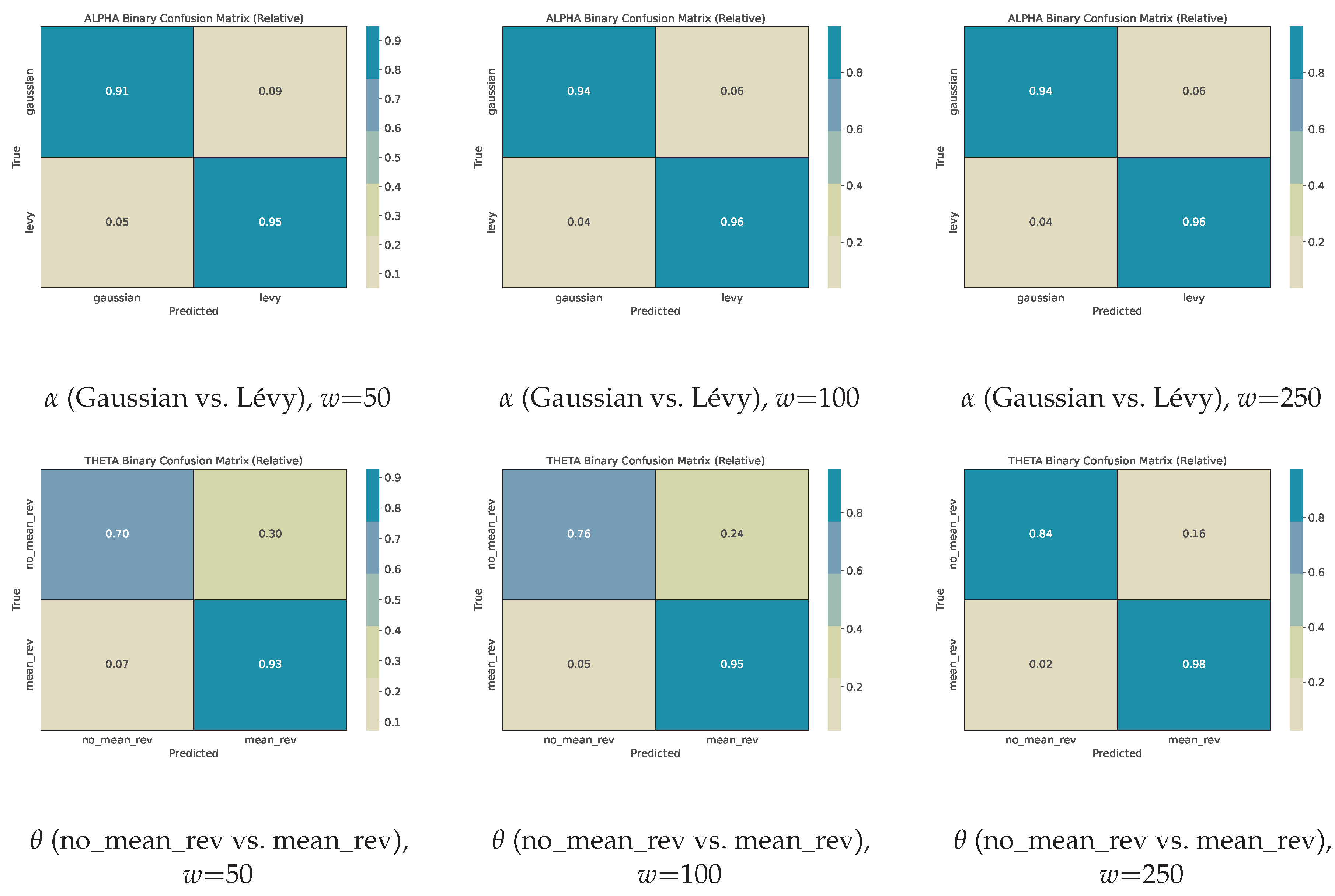
The row-normalized confusion matrices show diagonal dominance at all window sizes and a tighter diagonal as w grows. For , longer windows increase the chance that rare, large deviations appear inside the window, which improves separation of very heavy-tailed and Gaussian regimes. For , longer windows expose more of the pull-to-mean pattern or the lack of it, which improves separation of reversion rates. Figure 4 and Figure 5 illustrate the shortest-window setting, while Figure 8 and Figure 9 show the strongest separation at .
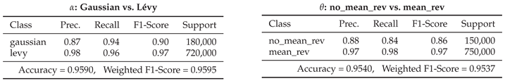
We also run a binary evaluation without retraining, using the same models and windows. For , we group non-Gaussian states into a single “Lévy” class and test “Gaussian vs. Lévy”; for , we test “no mean reversion () vs. mean reversion (all other ).” Full binary reports are provided in Appendix A. In short, the Gaussian vs. Lévy task reaches about 94–96% accuracy even at , and the no mean reversion vs. mean reversion task rises from about 89% to about 95% with window size. This indicates that the same trained models can be reused for coarse screening without additional fitting.
Overall, with independent-seed test sets and matched parameter grids, the models generalize consistently across window sizes. Multi-class errors are concentrated in neighboring labels, and the binary appendix confirms that the models provide reliable screening for Gaussian vs. non-Gaussian behavior and for mean reversion vs. no mean reversion.
5.1. Summary
The validation shows three main outcomes. First, the multiclass classifier separates very heavy-tailed and Gaussian regimes reliably, with most errors confined to neighboring intermediate tail classes. Second, the multiclass classifier benefits strongly from longer windows, indicating that mean-reversion strength requires more temporal context than tail classification in this setup. Third, the same models achieve high accuracy on the two binary tasks, supporting their use as window-based detectors for Gaussian vs. non-Gaussian behavior and mean reversion vs. no mean reversion in analyses.
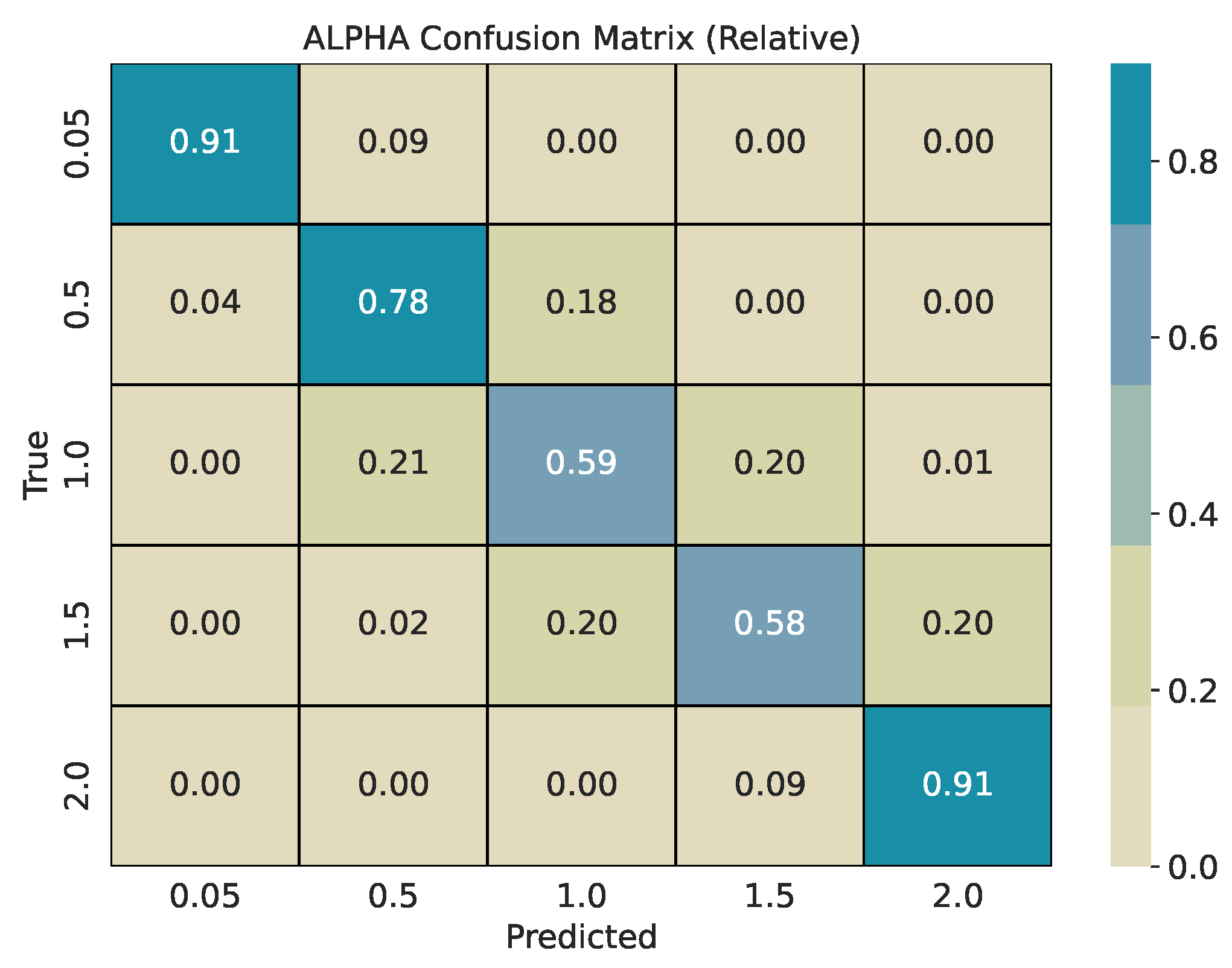
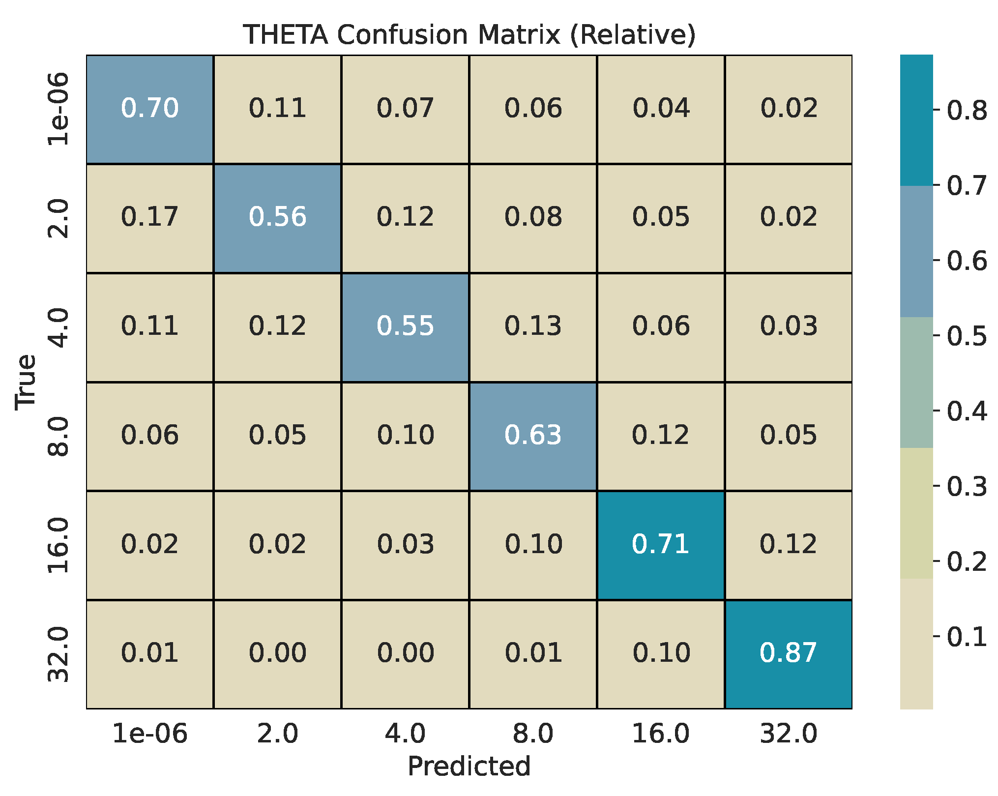
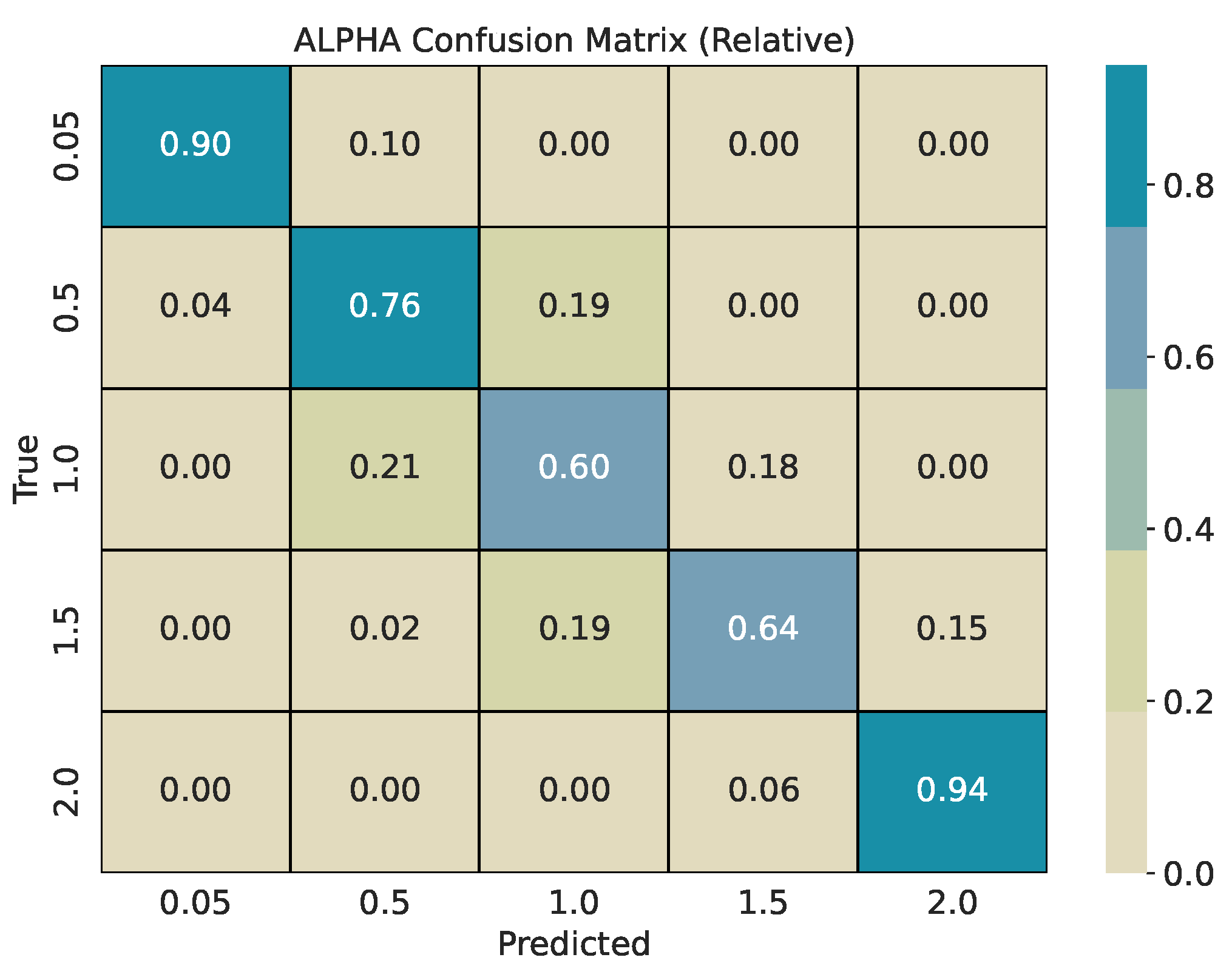
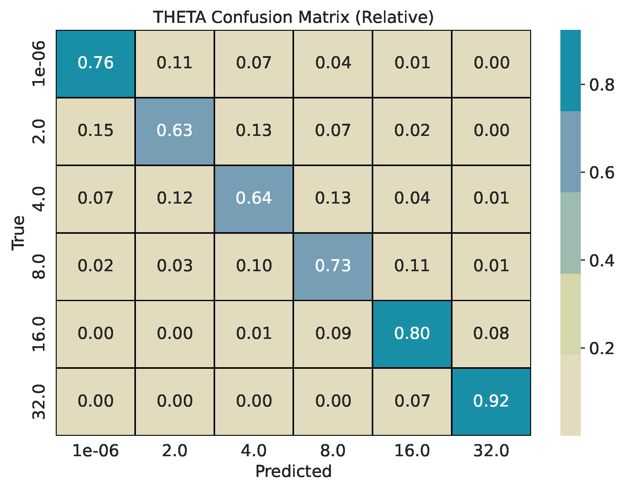
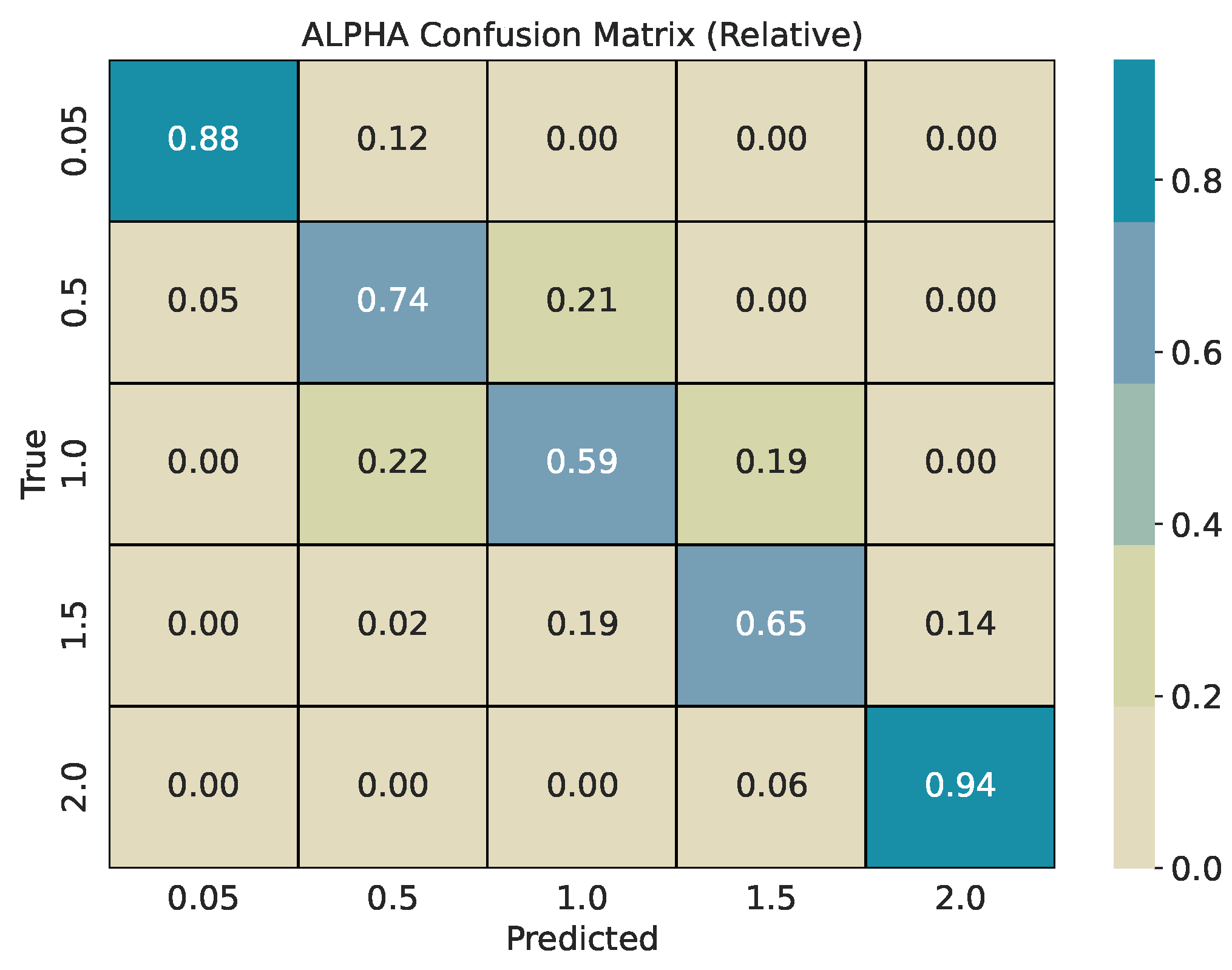
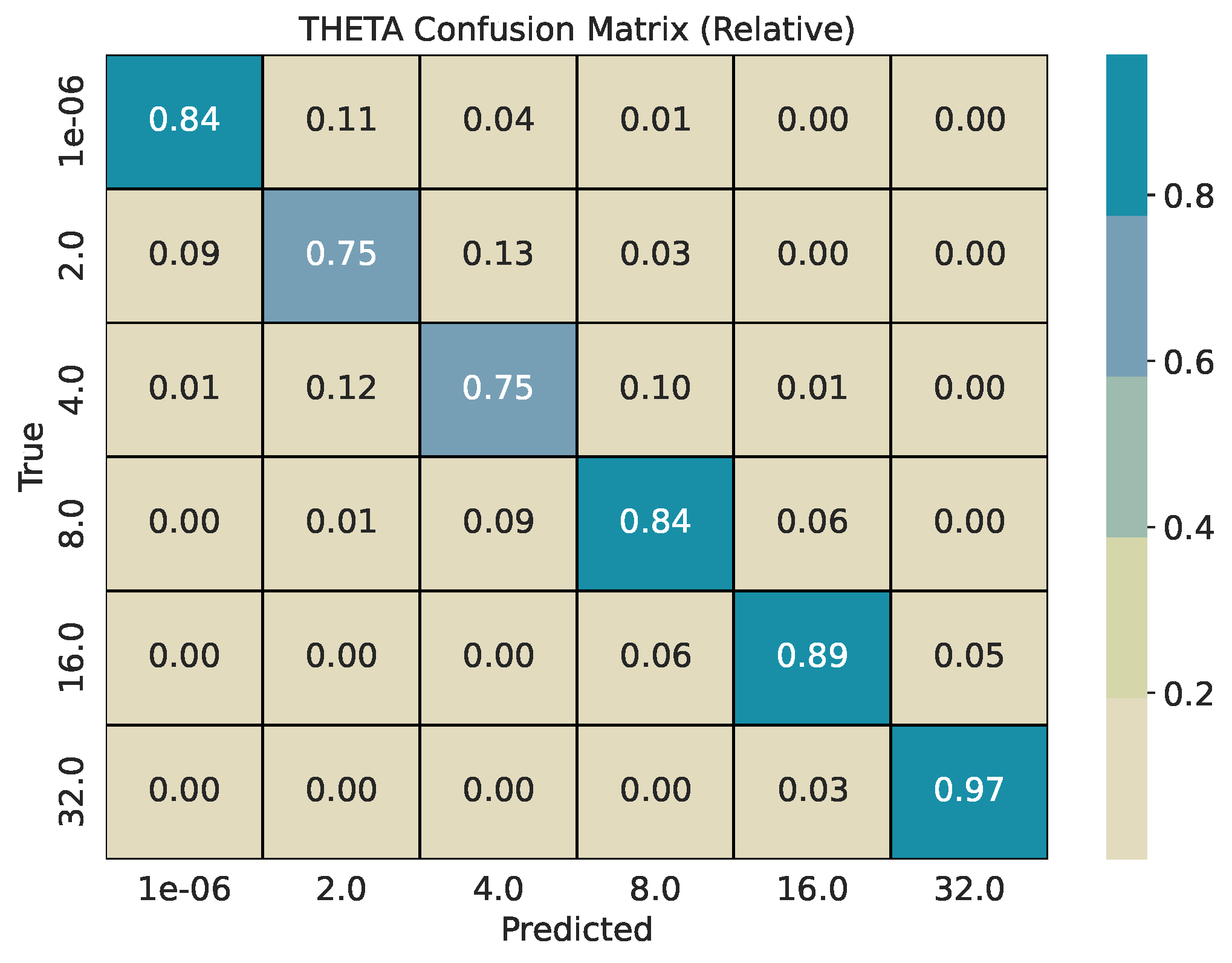

Table 1.
Classification Reports for Sliding Window of 50 Points.
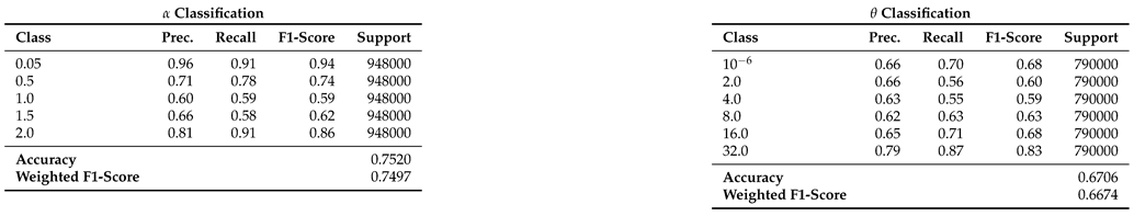 |
Table 2.
Classification Reports for Sliding Window of 100 Points.
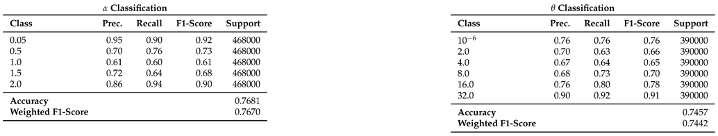 |
Table 3.
Classification Reports for Sliding Window of 250 Points.
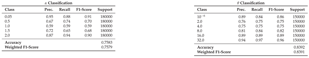 |
Figure 4.
Row-normalized confusion matrix for classification with a window size of 50.
Figure 5.
Row-normalized confusion matrix for classification with a window size of 50.
Figure 6.
Row-normalized confusion matrix for classification with a window size of 100.
Figure 7.
Row-normalized confusion matrix for classification with a window size of 100.
Figure 8.
Row-normalized confusion matrix for classification with a window size of 250.
Figure 9.
Row-normalized confusion matrix for classification with a window size of 250.
6. Daily Asset Data and Interval Comparison
Short-horizon distributional properties of financial returns are known to vary across market regimes and across assets. Heavy tails, volatility persistence, and state-dependent dependence structures are well-documented empirical features [6,40]. These characteristics can shift over time in response to changes in market microstructure, liquidity, or macroeconomic conditions [41]. Because our machine-learning models infer tail behavior () and mean-reversion strength () from short windows, applying them to long daily time series allows us to examine whether the relative prevalence of distributional regimes has changed across decades. This situates the method within a broader empirical literature on evolving market structure and non-Gaussian return behavior.
We analyze daily end-of-day price series for four representative assets: Apple (AAPL), Microsoft (MSFT), the S&P 500 (GSPC), and the Dow Jones Industrial Average (DJI). The history is divided into two non-overlapping intervals:
These intervals are selected to provide sufficiently long, contiguous samples for all assets and to contrast an earlier market environment with a more recent one. In practice, we chose them because they offer large and symmetric time spans with virtually no missing data for all four assets, i.e., primarily for reasons of data availability. All results are reported per asset and per interval.
To extract local distributional structure, each series is scanned using a sliding window of length 50 with step size 1. For every window, the trained classifiers assign one category for the stability index and one for the mean-reversion rate . This produces a categorical trace per asset. For each interval, we count how many windows fall into each discrete or bin. Figure 10 and Figure 11 summarize the annualized distribution of category assignments, and Table 4 and Table 5 provide absolute bin counts for each asset and interval. The binary classification tables are collected in Appendix B.
Table 4 and Table 5 summarize the number of windows classified into each or category. These counts provide a coarse view of how the empirical distribution of local regimes changes between intervals.
Interpretation.
Two consistent shifts appear when comparing Period 1 and Period 2. First, both broad indices (DJI, GSPC) show a notable reduction in windows classified as Gaussian (), with a corresponding increase in . AAPL and MSFT exhibit only modest changes. This indicates that index-level returns display heavier effective tails in the post-2010 sample, aligning with documented findings that aggregate markets can experience structural shifts in volatility and tail behavior [6,40].
Second, windows classified into the strongest mean-reversion state () decline for all assets except MSFT. This shift is consistent with a regime in which large deviations occur more frequently and take longer to dissipate, reducing the prevalence of tight, high-frequency mean reversion. These patterns do not contradict informational efficiency: EMH does not require Gaussianity [42,43]. Rather, they indicate that distributional characteristics of returns can evolve even when markets remain informationally efficient.
7. Daily Sunspot Data and Interval Comparison
Short-term statistical properties of solar activity are known to vary across solar cycles, including changes in dispersion, intermittency, and persistence [21,44]. These variations reflect the underlying solar magnetic dynamo and its modulation across decades. Because our machine-learning models quantify local tail behavior () and local mean-reversion strength (), applying the method to long daily sunspot records allows us to examine whether the prevalence of these regimes shifts systematically across different phases of solar activity. This links the analysis to empirical studies documenting structural differences between strong and weak solar cycles and motivates the use of short-window statistical diagnostics as complementary indicators of cycle-dependent behavior.
The daily international sunspot number series, published by SILSO (Sunspot Index and Long-term Solar Observations), provides a standardized measure of solar magnetic activity corrected for observational biases [45,46]. The time series reflects the emergence, evolution, and decay of sunspot groups and exhibits the well-known -year cycle. For this study, the record is divided into two non-overlapping intervals:
These intervals were selected primarily based on data availability: they are long, contiguous segments with no missing observations and can be split into two approximately symmetric parts that permit a comparison between an earlier phase dominated by relatively strong solar cycles 22–23 and a later phase that includes the deep minimum between cycles 23 and 24, the comparatively weak solar cycle 24, and the early phase of solar cycle 25 [21,44,47]. All results are reported per interval. For clarity, the solar cycles discussed here span the following official SILSO/NOAA intervals: Cycle 22 (1986–1996), Cycle 23 (1996–2008), Cycle 24 (2008–2019), and Cycle 25 (2019–present).
To extract local statistical regimes, the daily series is scanned with a sliding window of length 50 and step size 1. Each window is assigned an category (gaussian or levy) and a category (mean_rev or no_mean_rev) using the same trained models applied in the financial analysis. This produces two binary categorical sequences that summarize local tail behavior and local persistence. Annual counts of these binary categories are shown in Figure 12 for and Figure 13 for . Both use logarithmic scaling for the category counts and overlay the yearly average sunspot number for reference. Figure 12: The gaussian category peaks near solar maxima, indicating that high-activity phases are dominated by many moderate, approximately symmetric fluctuations. In contrast, levy windows cluster more strongly around solar minima, where long quiet intervals are punctuated by intermittent larger changes, yielding heavier tails. The transition from cycles 22–23 to the weaker cycle 24 and early cycle 25 is visible as a relative increase in levy windows during the later decades, consistent with more irregular and intermittent activity.
Figure 13: Years with high sunspot activity are dominated by mean_rev windows, indicating that local deviations tend to be rapidly corrected during strong cycles. Around extended minima and in the weaker recent cycles, the share of no_mean_rev windows increases, reflecting slower return toward equilibrium and more persistent deviations. The co-variation of these counts with the sunspot cycle suggests that local mean-reversion strength is itself a cycle-dependent property of the solar dynamo.
Interval-level totals are reported in Table 6 and Table 7. These aggregated counts complement the annual dynamics by showing how the relative frequencies of distributional and dynamical regimes change across the two multi-cycle periods.
The earlier interval (1985–2004) is dominated by windows classified as Gaussian and mean reversion. This suggests that local increments tend to be moderate, symmetric, and quickly corrected, consistent with the relatively strong and regular solar cycles characterizing this period. High-activity cycles naturally generate many small fluctuations driven by frequent sunspot emergence, producing distributions closer to Gaussian and dynamics consistent with strong mean reversion.
The later interval (2005–2024) shows a clear increase in levy-classified windows, rising from 2500 to 3575. This shift indicates heavier-tailed short-term changes, consistent with the long quiet stretches and intermittent bursts observed in weaker and more irregular cycles (especially the deep minimum between cycles 23 and 24 and the comparatively weak cycle 24). The -classification aligns with this pattern: the number of no_mean_rev windows increases substantially, implying that deviations persist longer and the process exhibits weaker corrective dynamics. Such behavior reflects the extended minima, asymmetric cycle shapes, and lower amplitudes documented in recent solar activity [21,44].
These findings form a coherent picture. Stronger cycles tend to generate frequent moderate fluctuations, leading to Gaussian-like and mean-reverting local dynamics. Weaker cycles produce intermittent, larger deviations that increase heavy-tailed behavior and decrease local mean reversion. Importantly, observing these differences is not only consistent with known solar-cycle variability but also valuable for future inference. If only short-window statistics ( and ) are available, the observed combination of heavier tails and weaker mean reversion provides evidence that the system is in a quieter and more irregular cycle, whereas predominantly Gaussian and mean-reverting behavior indicates a more active and regular phase. Since the intervals were intentionally chosen to contrast such regimes, the presence of clear statistical differences supports the usefulness of these local diagnostics for identifying the dynamical state of the solar cycle.
8. NASA POWER Daily Data for Austria
Daily reanalysis-based surface climate data provide a practical testbed for our regime-classification framework. They combine long, homogeneous time series with physically interpretable variables that are relevant for energy planning, agriculture, and impact studies [48,49,50]. Austria is a suitable case because it spans complex topography and continental-to-alpine climate gradients within a relatively small area, so that changes in short-horizon variability can be compared consistently across diverse conditions. By applying the classification to multi-decadal NASA POWER records, we assess whether the method recovers known contrasts between strongly forced and weather-modulated variables and whether it detects systematic shifts between two long, symmetric calendar intervals.
The Austrian surface-climate dataset analyzed here is derived from NASA’s POWER (Prediction Of Worldwide Energy Resources) project. POWER is an operational dissemination service hosted at NASA Langley Research Center that delivers solar and meteorological surface variables for energy, agrometeorology, and research applications, with consistent units, harmonized time standards, and long, gap-free coverage [48,50]. We retrieve daily records for a dense network of Austrian locations spanning all federal states—major urban centers (Vienna, Graz, Linz, Salzburg, Innsbruck, Klagenfurt, Bregenz), representative alpine valleys and high-elevation sites, and rural lowlands across Lower/Upper Austria, Styria, Carinthia, Tyrol, Vorarlberg, Salzburg, and Burgenland. Each site contributes a multi-decadal series from 1985-01-01 to 2024-12-31 for the variables used in this study: all-sky, clear-sky, and top-of-atmosphere shortwave irradiance; 10 m mean and daily-maximum wind speed; 2 m relative humidity; bias-corrected daily precipitation total; surface pressure; diurnal temperature range; and 2 m dew/frost-point temperature. The Daily API and its query parameters are documented at power.larc.nasa.gov/docs/services/api/temporal/daily/.
POWER provides point values by spatially sampling and interpolating authoritative gridded sources. For the parameters used here: (i) the meteorological variables (e.g., pressure, humidity, temperatures, winds, precipitation) originate from the NASA GMAO MERRA-2 reanalysis [49]; (ii) the surface and TOA radiative fields are sourced from the CERES (Clouds and the Earth’s Radiant Energy System) family of radiation products (CERES-SYN1deg and FLASHFlux), specialized for near-surface energy applications [51]. At delivery time, POWER harmonizes units—e.g., solar irradiance in MJ m−2 day−1—and applies standard formatting and metadata. A concise provenance summary for POWER, which lists MERRA-2 for meteorology and CERES-SYN1deg/FLASHFlux for radiation, along with product lineages and links to upstream documentation, is provided at power.larc.nasa.gov/data-sources.
Within POWER, PRECTOTCORR is a daily bias-corrected precipitation total designed for surface applications; radiation variables include ALLSKY_SFC_SW_DWN (all-sky surface shortwave on a horizontal plane), CLRSKY_SFC_SW_DWN (clear-sky surface shortwave), and TOA_SW_DWN (top-of-atmosphere shortwave), all provided as daily totals in MJ m−2 day−1 Wind fields (WS10M, WS10M_MAX) are in m s−1, humidity in %, pressure in kPa, diurnal temperature range in °C, and dew/frost-point in °C. The POWER Parameter Dictionary documents the full variable set, naming, units, and community-specific conventions, and is the reference for parameter semantics used in this work: power.larc.nasa.gov/docs/services/api/parameters/.
From a data-generation standpoint, MERRA-2 is NASA’s modern global atmospheric reanalysis produced by the Global Modelling and Assimilation Office (GMAO). It assimilates a wide range of satellite and in-situ observations into the GEOS modelling system to yield a spatially and temporally consistent estimate of atmospheric state and fluxes from 1980 to the present [49]; POWER serves MERRA-2-based surface meteorology at a daily cadence suitable for agrometeorological and energy applications [48]. The POWER data-source documentation summarizes this linkage and provides upstream references to GMAO and the CERES radiation suite (SYN1deg for consistent climate records; FLASHFlux for low-latency fluxes). Users should consult that page for details on spatial resolution, updates, and cross-product consistency: power.larc.nasa.gov/data-sources.
To characterize short-scale regime behavior consistently across variables and sites, each daily series is processed with a 50-day sliding window and step size of one day. For every window, we estimate the tail-heaviness and the mean-reversion . Windows are assigned to discrete bins of these two quantities, and absolute counts per category are accumulated over two multi-decadal intervals, 1985–2004 and 2005–2025. These intervals are chosen to be as long and symmetric as possible while maintaining uniform data availability for all locations and variables, so that changes in regime composition can be interpreted as temporal shifts rather than artifacts of coverage. The resulting distributions summarize how short-horizon dynamics change between the two periods, both for individual physical variables and for the full Austrian composite. A spatial overview of the analyzed locations is shown in Figure 14.
Following the spatial overview, we first present absolute counts by and category for all variables and both periods (Table 8 and Table 9). These tables provide the primary basis for comparing shifts in short-horizon regimes between the time periods 1985 to 2004 and 2005 to 2025. Complementary binary summaries that collapse categories into Gaussian vs. Lévy for and mean-reverting vs. non-mean-reverting for are reported in the Appendix (Table A6 and Table A7); they corroborate the main count patterns and are referenced in the discussion below.
Figure 15 highlights a marked redistribution in CLRSKY_SFC_SW_DWN around the year 2000: the annual share of Gaussian windows increases while Lévy windows drop; in parallel, mean-reverting windows become more dominant relative to non-mean-reverting ones. This visual change is consistent with the pooled counts in Table 8 and Table 9 and with the binary summaries in the Appendix (Table A6, Table A7), where CLRSKY shows a higher mass and a relative tilt toward stronger reversion in the timespan 2005 to 2025 compared to 1985 to 2004. The fact that these differences appear clearly in alone is useful for future applications: it implies that, when only short-window statistics are available, changes in the joint regime can be used as indicators of underlying shifts in the clear-sky radiative environment.
The aggregated counts across all Austrian locations reveal coherent and physically interpretable patterns. Radiative variables show strong contrasts between deterministic and weather-modulated components. The top-of-atmosphere shortwave flux (TOA_SW_DWN) concentrates almost entirely in the heaviest-tail side of the grid and in the weakest-reversion bins of in both periods, reflecting the smooth but non-stationary seasonal cycle: windows drift slowly along the annual irradiance envelope with little tendency to revert to a local mean, producing very low values and an apparent departure from Gaussianity. In contrast, the surface-level shortwave components (ALLSKY_SFC_SW_DWN, CLRSKY_SFC_SW_DWN) allocate much larger mass to and to high , consistent with faster short-term equilibration driven by day-to-day weather variability. Between periods, small but systematic redistributions are visible: for instance, counts rise for CLRSKY (395,689 vs. 310,660) and decreases slightly for ALLSKY (434,606 vs. 456,012), indicating a modest rebalancing between quickly mean-reverting, cloud-dominated variability and slowly varying seasonal components. These shifts are mirrored in the Appendix’s binary summaries, where CLRSKY shows more Gaussian and mean-reverting windows after 2005 (Table A6, Table A7). Because these shifts are captured directly in , they demonstrate that the framework can distinguish changes in short-horizon radiative behavior between multi-decadal periods using only local window statistics.
Wind variables (WS10M, WS10M_MAX) remain dominated by and strong mean reversion in both intervals, consistent with near-Gaussian daily increments and rapid synoptic-scale adjustment typical of mid-latitude surface winds. The mild shift from toward after 2005 points to slightly heavier tails—occasional stronger gust events—but the profile remains heavily concentrated in the fastest reversion class, implying that such excursions decay quickly at the 50-day scale.
Precipitation (PRECTOTCORR) is distinct in showing persistent heavy tails with concentrated around 1.0–1.5 and appreciable counts in 0.5. This reflects the intermittency and skewed nature of rainfall series, where dry spells alternate with bursts of wet days. Its -profile, while still anchored by high-reversion bins, includes non-trivial counts at weaker , consistent with multi-day weather regimes or blocked patterns that maintain elevated precipitation probabilities over several days.
Thermodynamic fields—surface pressure, relative humidity, dew-point temperature, and diurnal temperature range—show the opposite signature. These variables concentrate almost entirely in the Gaussian, fast-reverting regime. Surface pressure and humidity display high and , reflecting small, symmetric day-to-day fluctuations about a slowly varying mean. Dew-point temperature behaves similarly but with slightly broader tails, while diurnal range exhibits the strongest mean-reversion of all variables, with more than windows classified at in each period, indicating extremely rapid recovery of short-term anomalies.
Across all variables, three consistent themes emerge. Deterministically forced quantities such as top-of-atmosphere radiation remain structurally heavy-tailed and weakly reverting at this window scale. Weather-modulated fields—radiation near the surface, wind, and precipitation—occupy intermediate regimes where the balance between intermittency and reversion depends on local processes and changes only subtly between the two periods. Thermodynamic quantities remain stably Gaussian and fast-reverting, with minimal redistribution across decades. These patterns conform to established statistical characteristics of daily meteorological data and show that NASA POWER, with harmonized MERRA-2 inputs, reproduces these relations consistently across space and time. In this sense, the representation functions as a compact tool for analyzing short-horizon variability and for inferring regime shifts from local window statistics alone.
9. Discussion
Our goal is to recover two local, window–scale descriptors of dynamics, the stability (tail heaviness) and the mean-reversion rate , and to show that the same trained classifiers are useful across synthetic benchmarks and three real-world domains. Methodologically, the approach is best viewed as a tool: given a univariate time series and a choice of window length, it produces a categorical description of tail behavior and recovery speed without re-estimating a full stochastic model for each segment. The synthetic experiments establish that this tool can separate classes on controlled data; the financial, solar, and climate applications then illustrate how the same instrument behaves in applied settings, where “ground truth’’ is partial and domain knowledge must guide interpretation.
On synthetic, dimensionless Ornstein Uhlenbeck processes with -stable increments, we train separate CatBoost models for and on windows of length . The multi-class reports in Table 1, Table 2 and Table 3 and the confusion matrices in Figure 4, Figure 5, Figure 6, Figure 7, Figure 8 and Figure 9 show consistent generalization: accuracies increase with w, errors are predominantly between adjacent classes, and extremes are easiest to identify (e.g., and ; and ). The auxiliary binary evaluation (Appendix A) confirms that the same models, without retraining, act as reliable screeners: “Gaussian vs. Lévy’’ for reaches roughly 94–96% accuracy at and higher at longer windows, while “no_mean_rev vs. mean_rev’’ for rises from about 89% ( ) to about 95% ( ). These outcomes provide a controlled baseline for interpreting the real-data applications.
Applied to daily financial series (AAPL, MSFT, DJI, GSPC; Section 6), the window-level and maps indicate a post-2010 redistribution toward heavier effective tails and fewer occurrences of the strongest mean-reversion band in the broad indices, with more modest shifts for the two stocks. Concretely, counts fall for GSPC and DJI between 1995–2004 and 2010–2024, with mass moving largely to (Table 4); in parallel, counts decline for the indices and for AAPL, while MSFT remains closer to flat (Table 5). The annual traces in Figure 10 and Figure 11 visualize the same pattern. This is compatible with established “stylized facts’’ of asset returns, such as fat tails, volatility clustering, and scale-dependent dependence [5,6,52], and it does not contradict informational efficiency [42,43]. Rather, it echoes classic variance-ratio evidence that equity returns are positively autocorrelated at short horizons but negatively autocorrelated at multi-year horizons, implying a sizable transitory component and mean reversion over longer windows [8,52,53]. In our taxonomy, more windows labeled as heavy-tailed and fewer labeled as very fast-reverting mean that outlier moves occur more often and take longer to dissipate, especially in the indices after 2010.
A distinct episode visible across all annual and traces is the COVID-19 period (2020–2021). In each of the MSFT, GSPC, DJI, and AAPL panels, the onset of the pandemic coincides with a sharp increase in windows classified as heavy-tailed and a concurrent reduction in strongly mean-reverting windows, reflecting the abrupt and persistent volatility associated with the global shutdown and subsequent market reactions. The -based counts show a temporary shift toward the Lévy side, while the -based counts display fewer fast-reversion labels, consistent with slower dissipation of shocks during crisis conditions. This pattern is observable in all four assets despite their different long-term trajectories, indicating that the classifiers capture a coherent, system-wide regime disturbance. The clear COVID-19 signal illustrates that the method can detect short-horizon structural breaks and extreme periods directly from window-level dynamics, reinforcing its suitability as a tool for identifying regime changes in high-frequency financial time series.
Here the role of the tool is exploratory: it condenses large price archives into local “regime maps’’ that are consistent with known properties but are not tied to a single structural event.
For daily sunspot numbers (SILSO; Section 7), the two-interval comparison (1985–2004 vs. 2005–2024) shows a clear shift away from Gaussian-like windows toward heavier tails and a concurrent weakening of mean reversion. Interval counts move from 4805 Gaussian vs. 2500 Lévy in the time span from 1985 to 2004 to 3730 vs. 3575 in the next period from 2005 to 2024 (Table 6), while no_mean_rev rises from 2216 to 3311 windows (Table 7). The annual binary plots in Figure 12 and Figure 13 show that Gaussian and mean-reverting windows cluster near cycle maxima, whereas Lévy and non-reverting windows increase near minima. Interpreting the pair together: higher-activity cycles yield many small, quickly corrected fluctuations (more Gaussian, more mean reversion), while the weaker and more irregular cycles after 2005 present longer durations interrupted by intermittent bursts (heavier tails, weaker reversion).
For the Austrian NASA POWER dataset (Section 8), the accumulated counts across locations and variables (Table 8 and Table 9) separate three clear classes of behavior. The top-of-atmosphere shortwave downward irradiance (TOA_SW_DWN), which represents the incoming solar radiation before any atmospheric interaction, is governed almost entirely by deterministic orbital geometry. As a consequence, its 50-day windows fall predominantly into heavy-tailed, weak-reversion bins: within such short windows, the signal follows the seasonal cycle and exhibits slow drift with little short-term corrective dynamics. Surface-level shortwave irradiance under all-sky conditions (ALLSKY_SFC_SW_DWN) and clear-sky conditions (CLRSKY_SFC_SW_DWN), together with near-surface wind speed (WS10M, WS10M_MAX) and daily precipitation totals (PRECTOTCORR), reflect weather-modulated processes. Surface irradiance and wind fields show largely Gaussian, fast-reverting windows, indicating frequent short-term adjustments driven by synoptic variability. In contrast, precipitation exhibits persistent heavy tails and non-negligible counts in weaker-reversion classes, consistent with the intermittent alternation between dry spells and wet episodes typical of mid-latitude rainfall. Thermodynamic variables—surface pressure (PS), relative humidity at 2 m (RH2M), dew-point temperature (T2MDEW)—and the diurnal temperature range (T2M_RANGE) exhibit the opposite pattern. These quantities remain almost exclusively in the Gaussian, strongly mean-reverting regime, reflecting tight physical constraints and rapid synoptic adjustment. Their distributions show little redistribution across decades, consistent with their stable dynamical control. A notable finding is the redistribution in clear-sky surface shortwave irradiance (CLRSKY_SFC_SW_DWN) around the year 2000, visible in the annual binary splits (Figure 15). After 2000, windows labeled as Gaussian and mean-reverting become more frequent. This shift aligns with the period counts and binary summaries (Table A6 and Table A7). While not attributable to a single documented forcing event, the pattern illustrates how the method distinguishes between (i) deterministic seasonal drift (TOA irradiance), (ii) weather-driven variability (surface irradiance, winds, precipitation), and (iii) strongly regulated thermodynamic fields, using one consistent window-level diagnostic framework.
Across these three use cases, the role of the examples is therefore complementary. Financial series test whether the method recovers and refines well-known stylized facts. Sunspots provide a case where independent physical knowledge of cycle changes allows a qualitative external check. The Austrian climate fields illustrate how the same classifiers behave on multi-variable, spatially distributed data and how they separate deterministic and stochastic components. In all three settings, the tool does not “prove’’ specific causal stories; rather, it produces compact, interpretable summaries that can be compared with external knowledge and used to formulate hypotheses about regime changes, resilience, and control.
Across all domains, classifying and provides a operational summary: treat as a recovery meter and as a tail-risk meter. Trends toward lower with stable or heavier tails warn of slower recovery and more persistent deviations; trends toward higher with lighter tails indicate stabilization. Mixed signals call for domain checks (e.g., coupling changes, controls, measurement). This framing is consistent with early-warning theory in complex systems: as systems approach critical transitions, recovery slows, autocorrelation rises, and variance inflates [54,55,56]. Our window-level labels operationalize recovery speed, while labels track the potential for large shocks; together they translate information about a system’s resilience into measurable segments. Finally, our sensitivity analyses on synthetic data highlight an inherent limitation: finite windows impose unavoidable uncertainty, particularly for intermediate classes where local statistics overlap; increasing w reduces but does not eliminate near-neighbor confusions. In sum, the synthetic benchmarks show separability and accuracy of our approach, and the three real-world applications show that the same classifiers produce interpretable, domain-consistent classifications of tail behavior and recovery speed across markets, solar activity, and surface climate.
9.1. Larger-Scope Interpretation: Linking and to Real-World Systems
Our two parameters, the stability index and the mean-reversion rate , summarize complementary dimensions of local dynamics: how large typical fluctuations are, and how quickly a system returns toward equilibrium after a disturbance. Reading them together allows us to link the window-level patterns found in financial, solar, and climatic time series to broader mechanisms of variability, resilience, and control across complex systems.
When is large, perturbations decay rapidly and the system quickly reverts to baseline; when is small, deviations persist, and recovery slows. In the literature on critical slowing down, such declines in recovery speed and increases in short-lag autocorrelation have been interpreted as early-warning indicators of approaching tipping points [54,55,56]. In our analysis, extended runs of persistent mean reversion windows with declining effective therefore suggest weakening resilience, whereas stable or increasing implies a regime of fast equilibration. The results across all domains fit this intuition: synthetic and real systems with strong restoring forces, e.g., atmospheric pressure or diurnal temperature range, remain predominantly high-; those with slower or state-dependent feedbacks, e.g. precipitation, financial volatility, or solar activity—show more mass in weak-reversion bins and longer persistence of deviations.
The stability index quantifies the thickness of the tails: values near 2 indicate Gaussian-like noise with rare extremes, while smaller mark increasingly heavy tails, with higher probability of large jumps [5,6]. Heavy-tailed windows capture episodes where the variance of innovations is effectively infinite, implying bursts, jumps, or clustered extremes rather than steady diffusion. In markets, this corresponds to volatility clustering and drawdowns; in solar or climatic series, it maps to intermittent high-amplitude events (solar storms, intense precipitation). A shift toward higher may signal stabilization or averaging (e.g., due to stronger controls or measurement smoothing), while a decline toward lower points to more erratic, bursty regimes. We therefore interpret only jointly with : persistent heavy tails with low imply systems that both generate and retain large deviations, whereas heavy tails with high indicate frequent shocks but rapid recovery.
The financial results follow this logic. Equity returns show the well-documented pattern of positive short-horizon autocorrelation and negative long-horizon autocorrelation, implying transitory components and mean reversion [8,42,43,52,53]. In our maps, such behavior appears as alternating patches of mean_rev and no_mean_rev windows. The increase in heavy-tailed, weakly reverting intervals in indices after 2010 (Section 6) corresponds to periods of higher volatility and slower dissipation of shocks—consistent with post-crisis market structure changes and the persistence of macro volatility. Individual stocks, particularly AAPL and MSFT, show similar but less pronounced effects, suggesting partial insulation due to firm-specific growth factors.
The sunspot record provides a natural analog with a clear physical driver. Around each 11-year solar cycle maximum, the series exhibits many small, quickly corrected fluctuations, producing high and high ; near minima, activity becomes intermittent and clustered, lowering both parameters. Our counts and annual traces (Section 7) show that after 2005, the weaker, more irregular cycles coincide with a rise in Lévy and non-reverting windows, indicating a slower and more uneven recovery of solar activity after shocks. This matches known asymmetries and intermittency in modern solar cycles and supports interpreting as a dynamical recovery metric beyond classical variance measures.
The NASA POWER results (Section 8) extend this view to terrestrial climate fields. Deterministically forced quantities such as top-of-atmosphere shortwave flux concentrate in low-, heavy-tail bins, reflecting smooth seasonal drift with minimal stochastic correction. Near-surface variables—irradiance under clouds, winds, precipitation—occupy intermediate regimes where fast meteorological feedbacks coexist with intermittent forcing. The sharp redistribution in clear-sky surface shortwave irradiance (CLRSKY_SFC_SW_DWN) around 2000 (Figure 15) shows how large-scale radiative changes project onto local tail and reversion patterns: the post-2000 era displays more Gaussian and mean-reverting windows, potentially reflecting shifts in aerosol loading or cloud climatology. Thermodynamic fields such as pressure and humidity remain stably Gaussian and rapidly reverting, as expected under strong synoptic control. The binary appendices (Table A6 and Table A7) confirm that these categories are consistent across space and decades.
Taken together, the cross-domain synthesis suggests a simple operational reading. Treat as a recovery meter and as a tail-risk meter. Moving toward lower with stable or heavier tails signals slower recovery and higher persistence of shocks—an early-warning pattern observed in many complex systems [54,55]. Moving toward higher with lighter tails denotes stabilization and stronger feedback. Mixed signals, such as heavier tails but faster recovery, call for domain-specific interpretation (e.g., improved buffering or new controls masking underlying volatility). This joint perspective avoids over-interpreting any single metric and links our window-level classifications to the macroscopic behavior of markets, solar cycles, and climate systems. It also clarifies the role of the method in practice: not as a stand-alone detector of specific events, but as a compact diagnostic tool that turns long time series into interpretable maps of variability, recovery, and systemic risk.
10. Conclusions
We introduced a method to estimate the local mean-reversion rate and the stability index from time series using a feature-based, supervised learning framework trained on synthetic Ornstein–Uhlenbeck paths with -stable increments. The approach combines interpretable statistical descriptors with gradient-boosted classifiers to assign each short window of a real series to discrete categories. Synthetic benchmarks confirm that both parameters can be recovered with high accuracy and that confusion is largely confined to adjacent classes across window lengths.
Applying the same models to financial, solar, and climatic datasets shows that and capture different aspects of system dynamics in a consistent way. In financial returns, we find a redistribution between 1995–2004 and 2010–2024 toward heavier effective tails and fewer occurrences of the strongest mean-reversion band in the broad indices, with smaller changes for AAPL and MSFT. In solar activity, the comparison between 1985–2004 and 2005–2024 reveals that the weaker and more irregular recent cycles exhibit more Lévy-type and non-mean-reverting windows, while Gaussian and mean-reverting windows cluster around earlier cycle maxima. In the Austrian NASA POWER climate data, atmosphere radiation remains structurally heavy-tailed and weakly reverting, near-surface radiative and wind fields are largely Gaussian and fast-reverting, and thermodynamic variables are stably Gaussian and strongly mean-reverting; a clear redistribution in clear-sky shortwave irradiance around 2000 illustrates how large-scale radiative changes project onto respectively. In all three use cases, the method does not replace detailed physical or econometric modeling but acts as a compact diagnostic that produces domain-consistent categorizations of tail behavior and recovery speed.
Conceptually, the two parameters provide a simple operational reading: acts as a recovery meter and as a tail-risk meter. Trends toward lower with stable or heavier tails signal slower recovery and more persistent deviations, whereas higher with lighter tails indicates faster equilibration and reduced local tail risk. Because the classifiers operate directly on short windows and require only a generic feature representation, the framework is portable across domains and suitable for scanning long observational records for changes across short-horizon regimes.
This study has several limitations. First, the classifiers are trained on a specific synthetic family (dimensionless Ornstein–Uhlenbeck processes with symmetric -stable noise), so applications to systems with qualitatively different dynamics or strong asymmetries should be interpreted as phenomenological mappings rather than structural parameter recovery. Second, we work with finite window lengths and a discrete grid of classes; windows near class boundaries are intrinsically hard to distinguish, and some loss of information relative to continuous parameter estimates is unavoidable. Third, the feature set and CatBoost models were chosen for robustness and practicality, not optimality; other feature constructions or architectures might capture additional structure or yield different decision boundaries. Finally, all real-data case studies rely on external data products (financial indices, SILSO sunspot numbers, NASA POWER fields) with their own uncertainties and revisions, so our labels reflect both underlying dynamics and data-processing choices. These constraints do not invalidate the results but should be kept in mind when transferring the method to new domains or when using labels for operational decisions.
Future work should extend this approach to multivariate and spatiotemporal settings, integrate uncertainty estimates for the assignments, and investigate whether systematic shifts in the joint distribution of these labels can serve as early indicators of emerging transitions in economic, heliophysical, or climate-related systems.
The full code to reproduce our findings together with the trained models is available at
Author Contributions
Conceptualization, S.R.; methodology, S.R.; software, S.R.; validation, S.R., S.S., G.G., A.S. and K.M.; formal analysis, S.R., G.G.; investigation, S.R.; resources, S.S. and K.M.; data curation, S.R.; writing—original draft preparation, S.R., S.S., K.M., G.G. and A.S.; writing—review and editing, S.S., K.M., G.G. and A.S.; visualization, S.R.; supervision, S.S., A.S., and K.M.; project administration, S.S. and K.M.; funding acquisition, S.S. and K.M. All authors have read and agreed to the published version of the manuscript.
Funding
The financial support by the Austrian Federal Ministry of Economy, Energy and Tourism, the National Foundation for Research, Technology and Development and the Christian Doppler Research Association is gratefully acknowledged. SBA Research (SBA-K1 NGC) is a COMET Center within the COMET – Competence Centers for Excellent Technologies Programme and funded by BMIMI, BMWET, and the federal state of Vienna. The COMET Programme is managed by FFG. The authors acknowledge the funding by University of Vienna for financial support through its Open Access Funding Program
Use of Artificial Intelligence
We used Grammarly and ChatGPT to review the manuscript for grammar issues, typographical errors, and clarity. The tools were also used to improve the overall LaTeX presentation. All scientific content, interpretations, and conclusions reflect the authors’ work and judgment.
Data Availability Statement
Data openly available through APIs as shown in our corresponding repository at https://github.com/Raubkatz/HeavyTailsMeanReversion.
Conflicts of Interest
The authors declare no conflict of interest.
Appendix A. Extended Validation: Binary Tasks (Gaussian vs. Non-Gaussian; Strong vs. Weak Mean Reversion)
To complement the multi-class evaluation, we re-cast both problems as binary decisions and test the same trained models without retraining: (i) Gaussian vs. Lévy for (where the positive class “Gaussian” corresponds to , and “Lévy” aggregates ), and (ii) Strong mean reversion vs. Weak/No mean reversion for (where “mean_rev” aggregates and “no_mean_rev” corresponds to ). These binary diagnostics are practically useful: in many applications it suffices to know whether a window is approximately Gaussian (vs. heavy-tailed) or strongly mean-reverting (vs. weak), and such coarse screening can be more robust than fine-grained multi-class labeling.
Across window sizes, the Gaussian vs. Lévy task is learned very effectively. At , accuracy is (weighted ), with high recall for the Gaussian class () and excellent precision/recall for the Lévy class (). As the window grows to and , performance tightens further (accuracy –), reflecting the increased chance to observe tail behavior and volatility clustering within a longer segment. For mean reversion, the binary split is more challenging at smaller windows but improves substantially with w: at we attain accuracy (weighted ) with lower recall for no_mean_rev ()—reasonable given that weak reversion is expressed by an absence of pull, which is harder to certify in short segments. By the scores rise (accuracy ), and at the classifier reaches accuracy with balanced precision/recall for both classes (–). In short, longer windows sharpen both binary tasks, but even already delivers strong Gaussian screening and useful mean-reversion flags.
3×2 composite of binary confusion matrices.
Figure A1 collects the six binary confusion matrices (absolute counts at left, row-normalized at right within each panel is optional; here we show one panel per task and window size). Replace file names with your binary CM outputs.
Figure A1.
Binary confusion matrices (3×2 grid). Top row: (Gaussian vs. Lévy). Bottom row: (no_mean_rev vs. mean_rev). Each panel may be absolute or row-normalized; use consistent formatting across panels for readability.
Figure A1.
Binary confusion matrices (3×2 grid). Top row: (Gaussian vs. Lévy). Bottom row: (no_mean_rev vs. mean_rev). Each panel may be absolute or row-normalized; use consistent formatting across panels for readability.
Appendix A.0.1. Binary Classification Reports
We mirror the formatting of the multi-class section: for each window size, (left) and (right) reports are shown side-by-side.
Table A1.
Binary reports for 50-point windows.
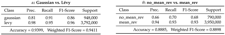 |
Table A2.
Binary reports for 100-point windows.
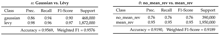 |
Table A3.
Binary reports for 250-point windows.
 |
Interpretation (binary).
For , the classifier is a reliable Gaussian screener: already at it distinguishes Gaussian windows from heavy-tailed alternatives with accuracy and balanced macro-averages, and it improves slightly with w. This indicates that the window-level complexity features capture distributional shape robustly, with longer windows providing more opportunities to observe tail events and intermittency. For , the binary split cleanly separates “presence” vs. “absence” of mean reversion by (accuracy ); at small w, weak reversion is harder to verify (lower recall for no_mean_rev), which is consistent with the temporal nature of reversion signals. Practically, these binary tests validate that the trained models can deliver crisp, interpretable flags (Gaussian vs. Lévy; strong vs. weak reversion) that align with the most consequential regime distinctions in downstream analyses.
Appendix B. Additional Results Financial Time Series Data
Table A4 and Table A5 report absolute counts per interval and asset for the binary versions of (Gaussian vs. Lévy) and (mean reversion vs. no mean reversion). Counts equal the number of rolling windows falling into each binary class within the given period.
Table A4.
Absolute binary counts for (Gaussian vs. Lévy) by period and asset.
| Period | Asset | Gaussian | Lévy | Rows |
|---|---|---|---|---|
| 1995–2010 | AAPL | 2297 | 1481 | 3778 |
| DJI | 2954 | 824 | 3778 | |
| GSPC | 2982 | 796 | 3778 | |
| MSFT | 2560 | 1218 | 3778 | |
| 2010–2024 | AAPL | 2325 | 1448 | 3773 |
| DJI | 2472 | 1301 | 3773 | |
| GSPC | 2451 | 1322 | 3773 | |
| MSFT | 2518 | 1255 | 3773 |
Table A5.
Absolute binary counts for (mean reversion vs. no mean reversion) by period and asset.
| Period | Asset | Mean reversion | No mean reversion | Rows |
|---|---|---|---|---|
| 1995–2010 | AAPL | 2290 | 1488 | 3778 |
| DJI | 2597 | 1181 | 3778 | |
| GSPC | 2584 | 1194 | 3778 | |
| MSFT | 2349 | 1429 | 3778 | |
| 2010–2024 | AAPL | 2412 | 1361 | 3773 |
| DJI | 2540 | 1233 | 3773 | |
| GSPC | 2492 | 1281 | 3773 | |
| MSFT | 2528 | 1245 | 3773 |
Appendix C. Additional NASA Power Data
Table A6.
Binary counts by period and variable (all Austrian locations pooled; 50-day windows, step 1).
Table A6.
Binary counts by period and variable (all Austrian locations pooled; 50-day windows, step 1).
| Period | Variable | Gaussian | Lévy | Rows |
|---|---|---|---|---|
| 1985–2004 | ALLSKY_SFC_SW_DWN | 252,661 | 273,299 | 525,960 |
| CLRSKY_SFC_SW_DWN | 310,660 | 215,300 | 525,960 | |
| PRECTOTCORR | 368 | 525,592 | 525,960 | |
| PS | 442,210 | 83,750 | 525,960 | |
| RH2M | 309,072 | 216,888 | 525,960 | |
| T2MDEW | 419,656 | 106,304 | 525,960 | |
| T2M_RANGE | 354,956 | 171,004 | 525,960 | |
| TOA_SW_DWN | 0 | 525,960 | 525,960 | |
| WS10M | 230,010 | 295,950 | 525,960 | |
| WS10M_MAX | 197,802 | 328,158 | 525,960 | |
| 2005–2025 | ALLSKY_SFC_SW_DWN | 267,713 | 258,247 | 525,960 |
| CLRSKY_SFC_SW_DWN | 395,689 | 130,271 | 525,960 | |
| PRECTOTCORR | 133 | 525,827 | 525,960 | |
| PS | 431,877 | 94,083 | 525,960 | |
| RH2M | 307,729 | 218,231 | 525,960 | |
| T2MDEW | 407,164 | 118,796 | 525,960 | |
| T2M_RANGE | 355,124 | 170,836 | 525,960 | |
| TOA_SW_DWN | 0 | 525,960 | 525,960 | |
| WS10M | 218,228 | 307,732 | 525,960 | |
| WS10M_MAX | 179,446 | 346,514 | 525,960 |
Table A7.
Binary counts by period and variable (all Austrian locations pooled; 50-day windows, step 1).
Table A7.
Binary counts by period and variable (all Austrian locations pooled; 50-day windows, step 1).
| Period | Variable | no_mean_rev | mean_rev | Rows |
|---|---|---|---|---|
| 1985–2004 | ALLSKY_SFC_SW_DWN | 8,878 | 517,082 | 525,960 |
| CLRSKY_SFC_SW_DWN | 158,849 | 367,111 | 525,960 | |
| PRECTOTCORR | 35,351 | 490,609 | 525,960 | |
| PS | 29,122 | 496,838 | 525,960 | |
| RH2M | 15,784 | 510,176 | 525,960 | |
| T2MDEW | 62,139 | 463,821 | 525,960 | |
| T2M_RANGE | 719 | 525,241 | 525,960 | |
| TOA_SW_DWN | 302,176 | 223,784 | 525,960 | |
| WS10M | 2,009 | 523,951 | 525,960 | |
| WS10M_MAX | 2,624 | 523,336 | 525,960 | |
| 2005–2025 | ALLSKY_SFC_SW_DWN | 11,134 | 514,826 | 525,960 |
| CLRSKY_SFC_SW_DWN | 188,429 | 337,531 | 525,960 | |
| PRECTOTCORR | 34,683 | 491,277 | 525,960 | |
| PS | 30,259 | 495,701 | 525,960 | |
| RH2M | 14,769 | 511,191 | 525,960 | |
| T2MDEW | 67,102 | 458,858 | 525,960 | |
| T2M_RANGE | 941 | 525,019 | 525,960 | |
| TOA_SW_DWN | 302,471 | 223,489 | 525,960 | |
| WS10M | 1,903 | 524,057 | 525,960 | |
| WS10M_MAX | 2,185 | 523,775 | 525,960 |
References
- Uhlenbeck, G.E.; Ornstein, L.S. On the Theory of the Brownian Motion. Physical Review 1930, 36, 823–841. Accessed: 2025-06-19. [CrossRef]
- Samorodnitsky, G.; Taqqu, M.S. Stable Non-Gaussian Random Processes: Stochastic Models with Infinite Variance, 1 ed.; Chapman & Hall: New York, 1994. Accessed: 2025-06-19. [CrossRef]
- Barndorff-Nielsen, O.E.; Shephard, N. Non-Gaussian Ornstein–Uhlenbeck-Based Models and Some of Their Uses in Financial Economics. Journal of the Royal Statistical Society: Series B 2001, 63, 167–241. Accessed: 2025-06-19. [CrossRef]
- Borovkov, K.; Decrouez, G. Ornstein–Uhlenbeck Type Processes with Heavy Distribution Tails. arXiv preprint arXiv:1102.5606 2011, [arXiv:math.PR/1102.5606]. Accessed: 2025-06-19. arXiv:1102.5606.
- Mandelbrot, B.B. The Variation of Certain Speculative Prices. The Journal of Business 1963, 36, 394–419. [CrossRef]
- Cont, R. Empirical properties of asset returns: stylized facts and statistical issues. Quantitative Finance 2001, 1, 223–236. Accessed on 2025-10-15. [CrossRef]
- Embrechts, P.; Klüppelberg, C.; Mikosch, T. Modelling Extremal Events: For Insurance and Finance, 1 ed.; Vol. 33, Applications of Mathematics, Springer: Berlin Heidelberg, 1997; pp. xv+648. Accessed on 2025-10-15. [CrossRef]
- Poterba, J.M.; Summers, L.H. Mean reversion in stock prices: Evidence and Implications. Journal of Financial Economics 1988, 22, 27–59. [CrossRef]
- Basel Committee on Banking Supervision. Principles for Sound Stress Testing Practices and Supervision. Basel Committee publication BCBS 155, Bank for International Settlements, Basel, 2009. May 2009. Accessed on 2025-10-15. Superseded by: Stress Testing Principles (17 Oct 2018).
- Basel Committee on Banking Supervision. Stress Testing Principles. Guidelines BCBS d450, Bank for International Settlements, Basel, 2018. Accessed on 2025-10-15. Publisher landing page; full text PDF available at https://www.bis.org/bcbs/publ/d450.pdf.
- Raubitzek, S.; Neubauer, T. An Exploratory Study on the Complexity and Machine Learning Predictability of Stock Market Data. Entropy 2022, 24. [CrossRef]
- Katz, R.W.; Parlange, M.B.; Naveau, P. Statistics of extremes in hydrology. Advances in Water Resources 2002, 25, 1287–1304. Listed as Volume 25, Issues 8–12 (Aug–Dec 2002) on the publisher page. [CrossRef]
- Wilks, D.S. Statistical Methods in the Atmospheric Sciences, 3 ed.; Vol. 100, International Geophysics, Academic Press, 2011. Hardback ISBN: 978-0-12-385022-5; published May 20, 2011.
- Lovejoy, S.; Schertzer, D. The Weather and Climate: Emergent Laws and Multifractal Cascades; Cambridge University Press: Cambridge, 2013; pp. xv+475. Accessed on 2025-10-14. [CrossRef]
- Nolan, J.P. Stable Distributions—Models for Heavy Tailed Data, 2 ed.; Springer Series in Operations Research and Financial Engineering, Birkhäuser: Cham, Switzerland, 2020. Accessed: 2025-06-19. [CrossRef]
- Basseville, M.; Nikiforov, I.V. Detection of Abrupt Changes: Theory and Application, 1 ed.; Prentice-Hall Information and System Sciences Series, Prentice Hall: Englewood Cliffs, NJ, 1993; pp. xxvi+528. Author-hosted full text: https://people.irisa.fr/Michele.Basseville/kniga/kniga.pdf, Accessed on 2025-10-14.
- Adams, R.P.; MacKay, D.J.C. Bayesian Online Changepoint Detection. arXiv preprint arXiv:0710.3742 2007, p. 7. Accessed on 2025-10-14. [CrossRef]
- Bandt, C.; Pompe, B. Permutation Entropy: A Natural Complexity Measure for Time Series. Physical Review Letters 2002, 88, 174102. Accessed: 2025-06-19. [CrossRef]
- Prokhorenkova, L.; Gusev, G.; Vorobev, A.; Dorogush, A.V.; Gulin, A. CatBoost: unbiased boosting with categorical features. In Proceedings of the Advances in Neural Information Processing Systems (NeurIPS), 2018, pp. 6638–6648, [arXiv:cs.LG/1706.09516]. Accessed on 2025-03-10.
- Dorogush, A.V.; Ershov, V.; Gulin, A. CatBoost: gradient boosting with categorical features support. In Proceedings of the Workshop on ML Systems at NeurIPS, 2017. Accessed on 2025-03-10.
- Hathaway, D.H. The Solar Cycle. Living Reviews in Solar Physics 2015, 12, 1–87. Review Article; published 21 Sep 2015 (Living Rev Solar Phys 12:4). [CrossRef]
- Raubitzek, S.; Neubauer, T. Combining Measures of Signal Complexity and Machine Learning for Time Series Analysis: A Review. Entropy 2021, 23. [CrossRef]
- Raubitzek, S.; Neubauer, T. Taming the Chaos in Neural Network Time Series Predictions. Entropy 2021, 23. [CrossRef]
- Raubitzek, S.; Neubauer, T. Reconstructed Phase Spaces and LSTM Neural Network Ensemble Predictions. Engineering Proceedings 2022, 18. [CrossRef]
- Raubitzek, S.; Neubauer, T.; Friedrich, J.; Rauber, A. Interpolating Strange Attractors via Fractional Brownian Bridges. Entropy 2022, 24. [CrossRef]
- Raubitzek, S.; Neubauer, T. A fractal interpolation approach to improve neural network predictions for difficult time series data. Expert Systems with Applications 2021, 169, 114474. [CrossRef]
- Mallinger, K.; Raubitzek, S.; Neubauer, T.; Lade, S. Potentials and limitations of complexity research for environmental sciences and modern farming applications. Current Opinion in Environmental Sustainability 2024, 67, 101429. Accessed on 2025-03-10.
- Gardiner, C.W. Handbook of Stochastic Methods for Physics, Chemistry and the Natural Sciences, 2 ed.; Springer Series in Synergetics, Springer: Berlin; Heidelberg; New York; Tokyo, 1985. Accessed: 2025-06-19. [CrossRef]
- Risken, H.; Haken, H. The Fokker–Planck Equation: Methods of Solution and Applications, 2 ed.; Springer Series in Synergetics, Springer-Verlag: Berlin; New York, 1989. Accessed: 2025-06-19. [CrossRef]
- Karatzas, I.; Shreve, S.E. Brownian Motion and Stochastic Calculus, 2 ed.; Vol. 113, Graduate Texts in Mathematics, Springer-Verlag: New York; Berlin, 1991. Accessed: 2025-06-19. [CrossRef]
- Marquardt, T. Fractional Lévy Processes with an Application to Long Memory Moving Average Processes. Bernoulli 2007, 13, 145–167. Accessed: 2025-06-19. [CrossRef]
- Virtanen, P.; Gommers, R.; Oliphant, T.E.; Haberland, M.; Reddy, T.; Cournapeau, D.; Burovski, E.; Peterson, P.; Weckesser, W.; Bright, J.; et al. SciPy 1.0: Fundamental Algorithms for Scientific Computing in Python. Nature Methods 2020, 17, 261–272. [CrossRef]
- SciPy Developers. scipy.stats.levy_stable — SciPy API Reference. https://docs.scipy.org/doc/scipy/reference/generated/scipy.stats.levy_stable.html. Accessed: 2025-06-20. [CrossRef]
- Chambers, J.M.; Mallows, C.L.; Stuck, B.W. A Method for Simulating Stable Random Variables. Journal of the American Statistical Association 1976, 71, 340–344. Accessed: 2025-06-20. [CrossRef]
- Quinlan, J.R. Induction of Decision Trees. Machine Learning 1986, 1, 81–106. [CrossRef]
- Breiman, L. Random Forests. Machine Learning 2001, 45, 5–32. Accessed on 2025-10-15. [CrossRef]
- Raubitzek, S.; Mallinger, K. On the Applicability of Quantum Machine Learning. Entropy 2023, 25. Accessed on 2025-03-10. [CrossRef]
- Raubitzek, S.; Corpaci, L.; Hofer, R.; Mallinger, K. Scaling Exponents of Time Series Data: A Machine Learning Approach. Entropy 2023, 25. Accessed on 2025-03-10. [CrossRef]
- Corpaci, L.; Wagner, M.; Raubitzek, S.; Kampel, L.; Mallinger, K.; Simos, D.E. Estimating Combinatorial t-Way Coverage Based on Matrix Complexity Metrics. In Proceedings of the Testing Software and Systems; Menéndez, H.D.; Bello-Orgaz, G.; Barnard, P.; Bautista, J.R.; Farahi, A.; Dash, S.; Han, D.; Fortz, S.; Rodriguez-Fernandez, V., Eds., Cham, 2025; pp. 3–20.
- Bouchaud, J.P.; Potters, M. Theory of Financial Risk and Derivative Pricing; Cambridge University Press, 2003.
- Lux, T. Long-term stochastic volatility and fat tails. Advances in Complex Systems 2004, 7, 1–23.
- Fama, E.F. Efficient Capital Markets: A Review of Theory and Empirical Work. The Journal of Finance 1970, 25, 383–417. [CrossRef]
- Fama, E.F. Efficient Capital Markets: II. The Journal of Finance 1991, 46, 1575–1617. [CrossRef]
- Usoskin, I.G. A History of Solar Activity over Millennia. Living Reviews in Solar Physics 2023, 20, 2. [CrossRef]
- Clette, F.; Lefèvre, L. International Sunspot Number (SN) Version 2.0, 2015. Published by WDC–SILSO (Sunspot Index and Long-term Solar Observations); license: CC BY-NC 4.0. [CrossRef]
- WDC–SILSO (SILSO World Data Center). SILSO: World Data Center for the production, preservation and dissemination of the International Sunspot Number. Royal Observatory of Belgium (ROB), Brussels, Belgium, 2025. Website of the WDC–SILSO service; data are released under CC BY-NC 4.0. For sunspot number data citation, SILSO requests citing the SN version and DOI (e.g., Version 2, DOI: 10.24414/qnza-ac80). [CrossRef]
- Miesch, M. Solar Cycle Progression Updated Prediction (Experimental): Validation Document. Technical report, NOAA Space Weather Prediction Center (SWPC); CIRES/University of Colorado, 2024. Last updated: 2024-01-18.
- NASA Langley Research Center. NASA POWER Project: Data Sources and Methodology. https://power.larc.nasa.gov/docs/methodology/data/sources/, 2025. Accessed: 2025-01-XX.
- Gelaro, R.; McCarty, W.; Suárez, M.J.; Todling, R.; Molod, A.; Takacs, L.; Randles, C.A.; Darmenov, A.; Bosilovich, M.G.; Reichle, R.; et al. The Modern-Era Retrospective Analysis for Research and Applications, Version 2 (MERRA-2). Journal of Climate 2017, 30, 5419–5454. [CrossRef]
- Stackhouse, P.W.; Zhang, T.; Westberg, D.; Barnett, A.J.; Bristow, T.; Macpherson, B.; Hoell, J.M. POWER Release 8 (with GIS Applications) Methodology (Data Parameters, Sources, & Validation), Data Version 8.0.1. NASA Prediction Of Worldwide Energy Resources (POWER) Project, NASA Langley Research Center, 2018. Primary methodology documentation for NASA POWER Release 8; the specific AGU Fall Meeting abstract-style citation is not consistently discoverable via non-JS sources, so this NASA-hosted technical document is the most verifiable citable item.
- Loeb, N.G.; Doelling, D.R.; Wang, H.; Su, W.; Nguyen, C.; Corbett, J.G.; Liang, L.; Mitrescu, C.; Rose, F.G.; Kato, S. Clouds and the Earth’s Radiant Energy System (CERES) Energy Balanced and Filled (EBAF) Top-of-Atmosphere (TOA) Edition 4.0 Data Product. Journal of Climate 2018, 31, 895–918. [CrossRef]
- Lo, A.W.; MacKinlay, A.C. Stock Market Prices Do Not Follow Random Walks: Evidence from a Simple Specification Test. The Review of Financial Studies 1988, 1, 41–66. [CrossRef]
- Fama, E.F.; French, K.R. Permanent and Temporary Components of Stock Prices. Journal of Political Economy 1988, 96, 246–273. [CrossRef]
- Dakos, V.; Scheffer, M.; van Nes, E.H.; Brovkin, V.; Petoukhov, V.; Held, H. Slowing down as an early warning signal for abrupt climate change. Proceedings of the National Academy of Sciences 2008, 105, 14308–14312. Accessed on 2025-10-15. [CrossRef]
- Scheffer, M.; Bascompte, J.; Brock, W.A.; Brovkin, V.; Carpenter, S.R.; Dakos, V.; Held, H.; van Nes, E.H.; Rietkerk, M.; Sugihara, G. Early-warning signals for critical transitions. Nature 2009, 461, 53–59. Accessed on 2025-10-15. [CrossRef]
- Lenton, T.M.; Livina, V.N.; Dakos, V.; van Nes, E.H.; Scheffer, M. Early warning of climate tipping points from critical slowing down: comparing methods to improve robustness. Philosophical Transactions of the Royal Society A: Mathematical, Physical and Engineering Sciences 2012, 370, 1185–1204. Accessed on 2025-10-15. Publisher page. [CrossRef]
Figure 1.
Overview of our approach: First, Left: Synthetic time series are generated from Ornstein–Uhlenbeck processes with varying mean–reversion strength and tail behavior to cover a wide range of Gaussian and non-Gaussian regimes. Center: A supervised learning model (CatBoost) is trained on these samples to learn how mean reversion and extreme-value behavior are expressed in short time windows. Right: The trained classifier is applied to real-world financial time series to validate the approach. The validation step shows how the method distinguishes windows with strong vs. weak reversion and Gaussian vs. heavy-tailed behavior in real-life data, e.g., financial and environmental data.
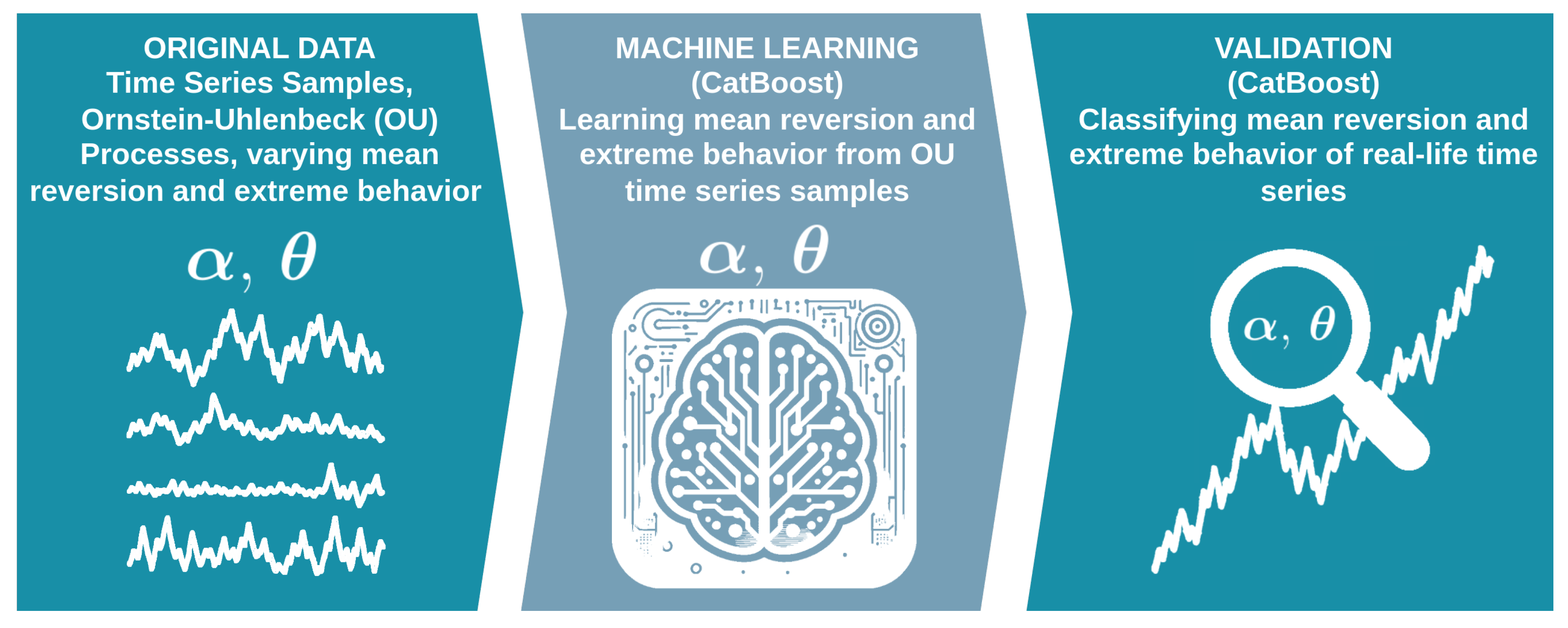
Figure 2.
Dimensionless OU sample paths with symmetric -stable innovations () for (panels (a)–(c)). Smaller produces heavier tails and more frequent large jumps. The mean-reversion rate and the sampling step are the same across panels.
Figure 2.
Dimensionless OU sample paths with symmetric -stable innovations () for (panels (a)–(c)). Smaller produces heavier tails and more frequent large jumps. The mean-reversion rate and the sampling step are the same across panels.
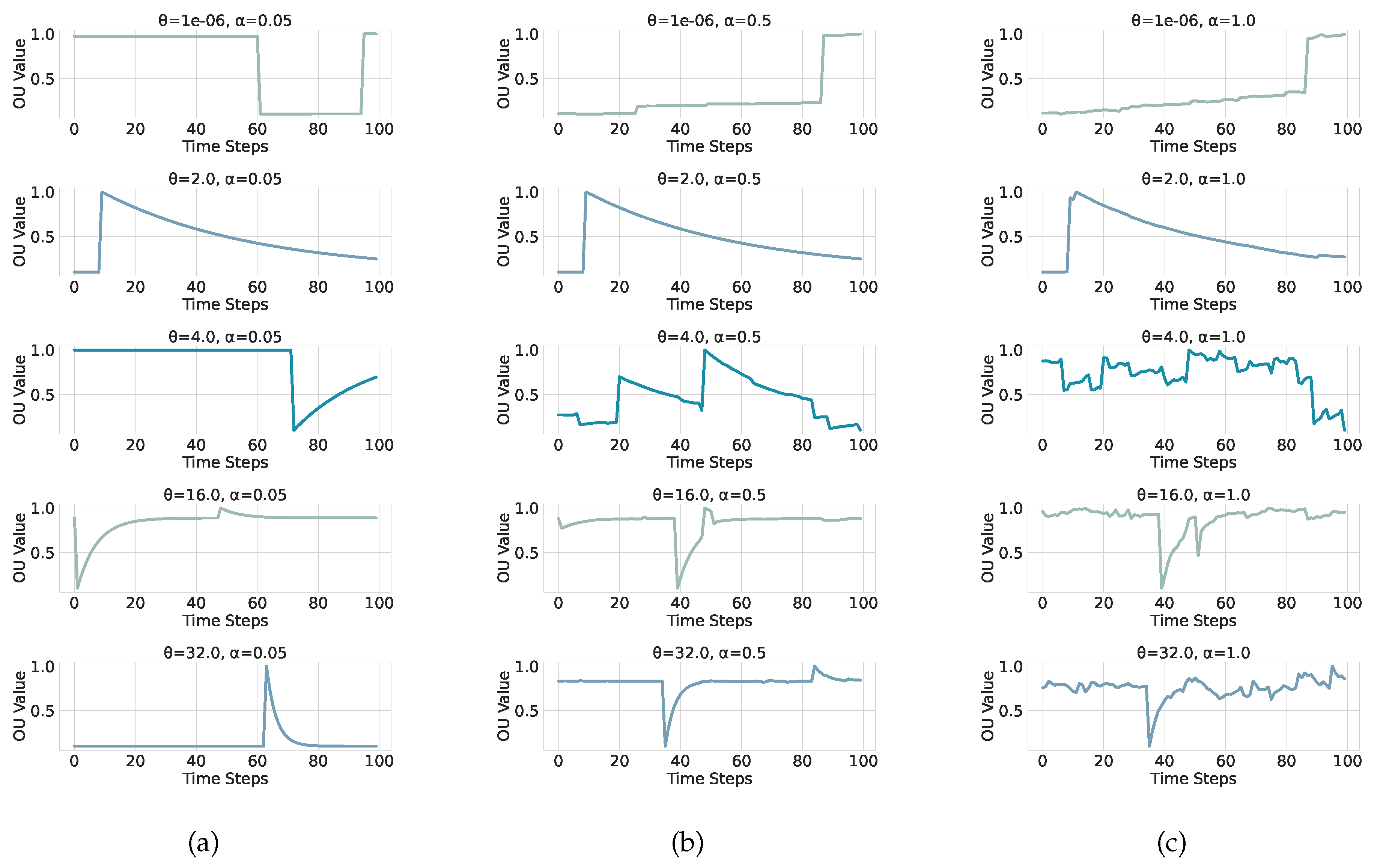
Figure 3.
Dimensionless OU sample paths with symmetric -stable innovations () for (panels (d)–(e)). The case corresponds to the Gaussian OU model. The mean-reversion rate and the sampling step are the same across panels.
Figure 3.
Dimensionless OU sample paths with symmetric -stable innovations () for (panels (d)–(e)). The case corresponds to the Gaussian OU model. The mean-reversion rate and the sampling step are the same across panels.
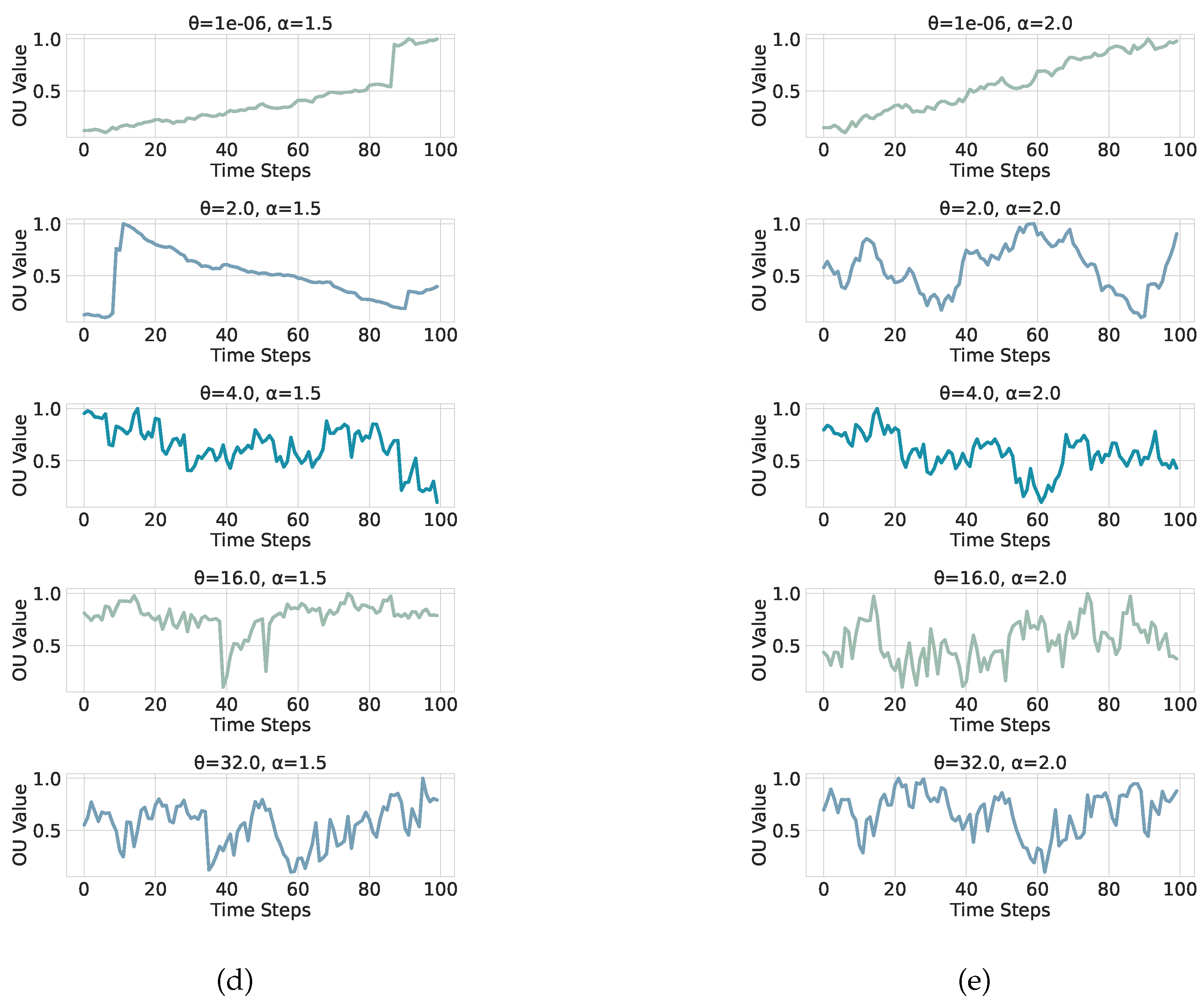
Figure 10.
Annual counts of regime labels (gaussian vs. levy) shown on a log scale.
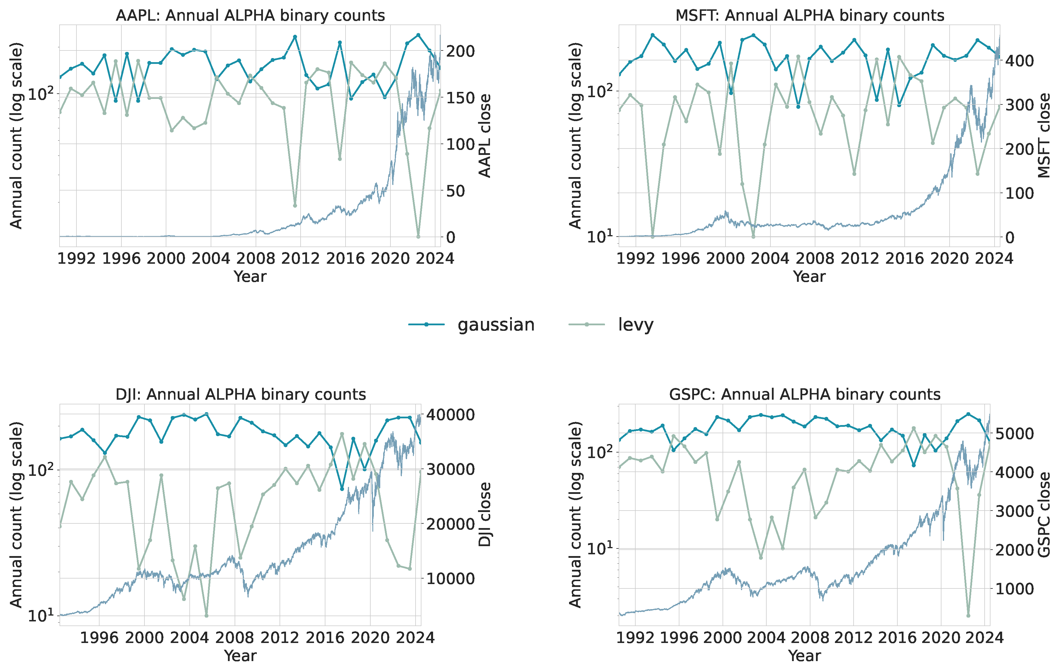
Figure 11.
Annual counts of regime labels (mean reversion vs. no mean reversion) on a log scale.
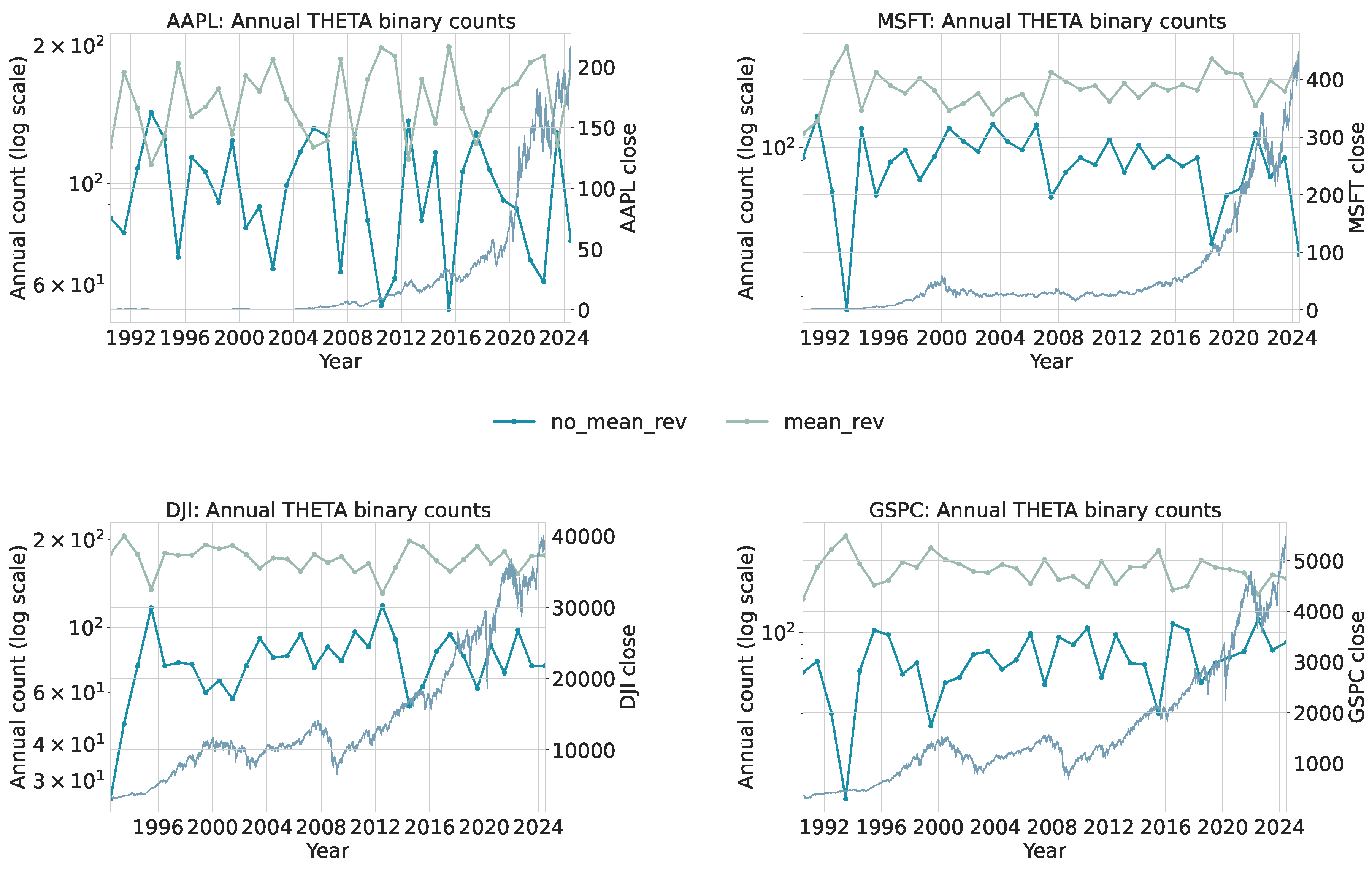
Figure 12.
Annual binary counts for regimes in the daily sunspot series. The plot shows categories (gaussian vs. levy) on a logarithmic count scale, with the yearly average sunspot number overlaid for reference.
Figure 12.
Annual binary counts for regimes in the daily sunspot series. The plot shows categories (gaussian vs. levy) on a logarithmic count scale, with the yearly average sunspot number overlaid for reference.
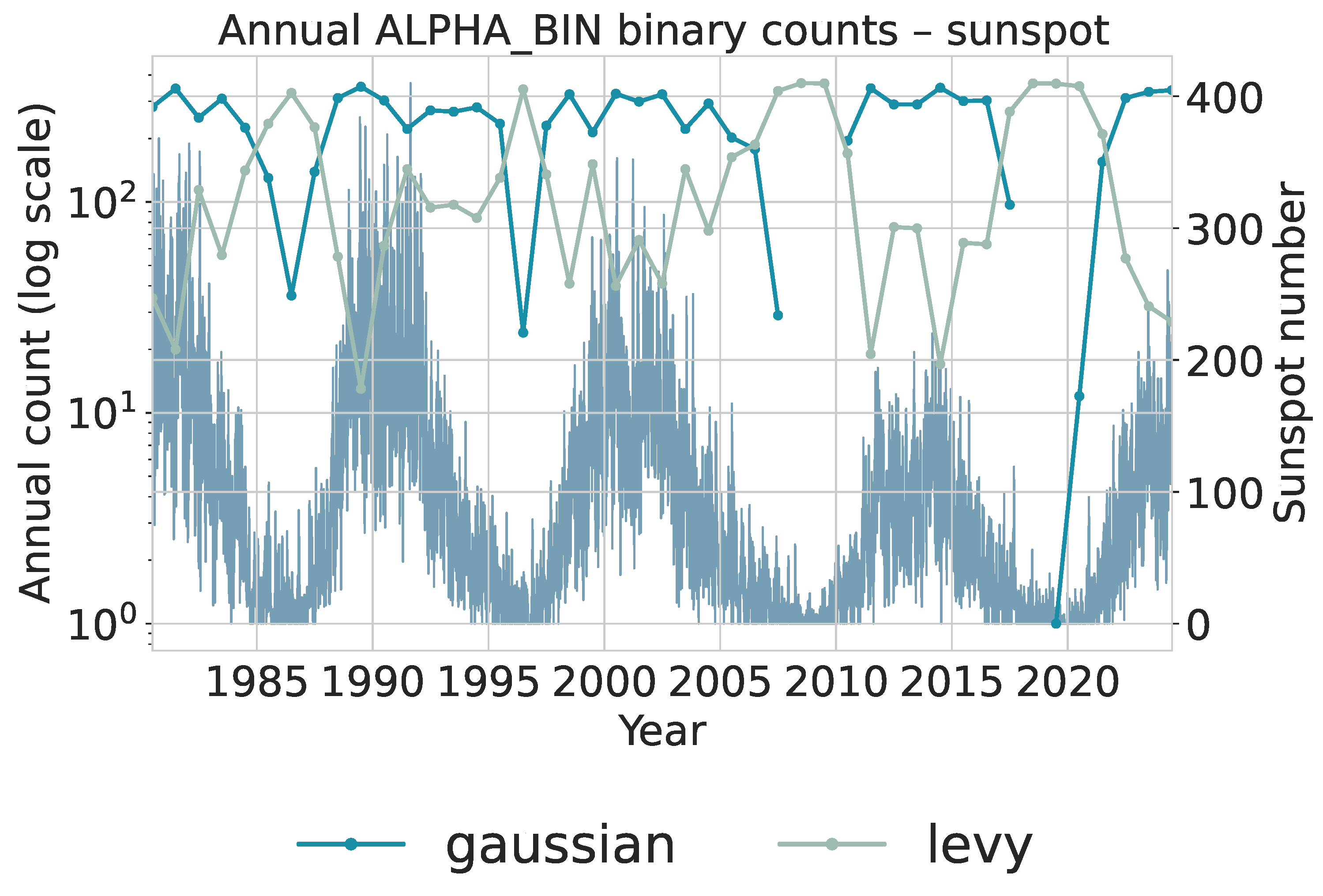
Figure 13.
Annual binary counts for regimes in the daily sunspot series. The plot shows categories (mean_rev vs. no_mean_rev) on a logarithmic count scale, again with the yearly average sunspot number overlaid for reference.
Figure 13.
Annual binary counts for regimes in the daily sunspot series. The plot shows categories (mean_rev vs. no_mean_rev) on a logarithmic count scale, again with the yearly average sunspot number overlaid for reference.
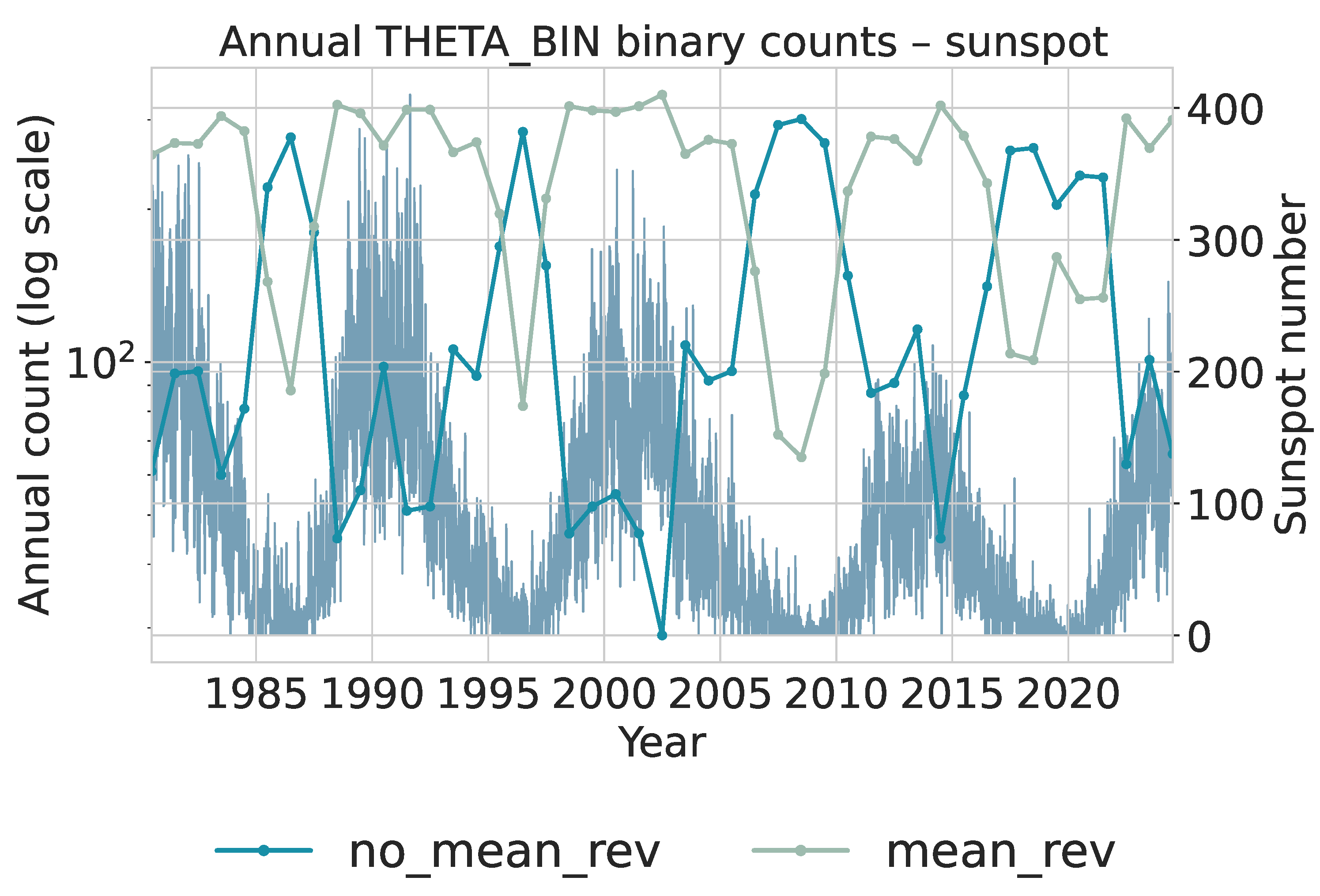
Figure 14.
Spatial coverage of the Austrian NASA POWER network used in this study. Each marker represents one daily site record extending from 1985 to 2024.
Figure 14.
Spatial coverage of the Austrian NASA POWER network used in this study. Each marker represents one daily site record extending from 1985 to 2024.
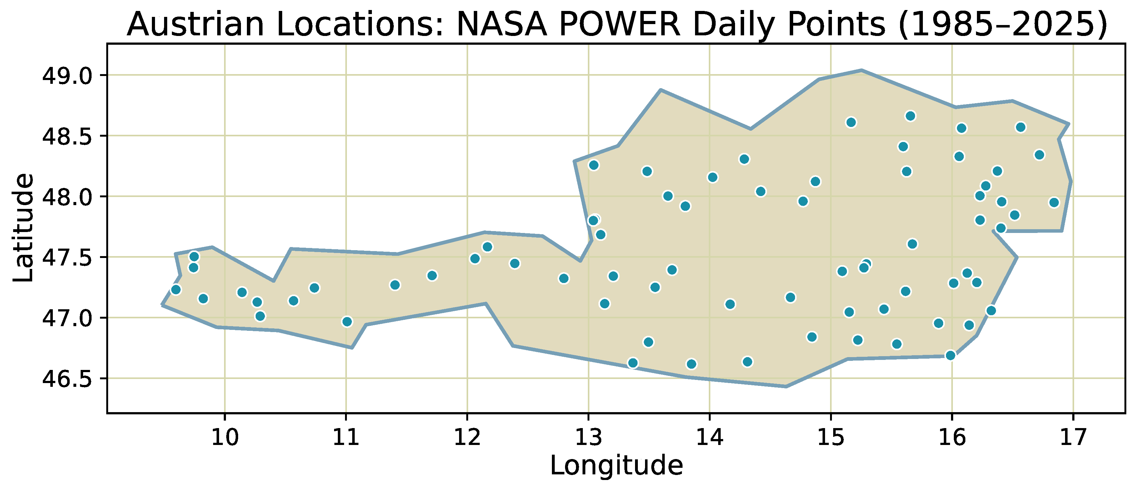
Figure 15.
Annual window counts for CLRSKY_SFC_SW_DWN on a log scale. Left: binary split (Gaussian vs. Lévy). Right: binary split (mean_rev vs. no_mean_rev). Both panels show a pronounced regime change around the year 2000, with a rising share of Gaussian and mean-reverting windows thereafter.
Figure 15.
Annual window counts for CLRSKY_SFC_SW_DWN on a log scale. Left: binary split (Gaussian vs. Lévy). Right: binary split (mean_rev vs. no_mean_rev). Both panels show a pronounced regime change around the year 2000, with a rising share of Gaussian and mean-reverting windows thereafter.
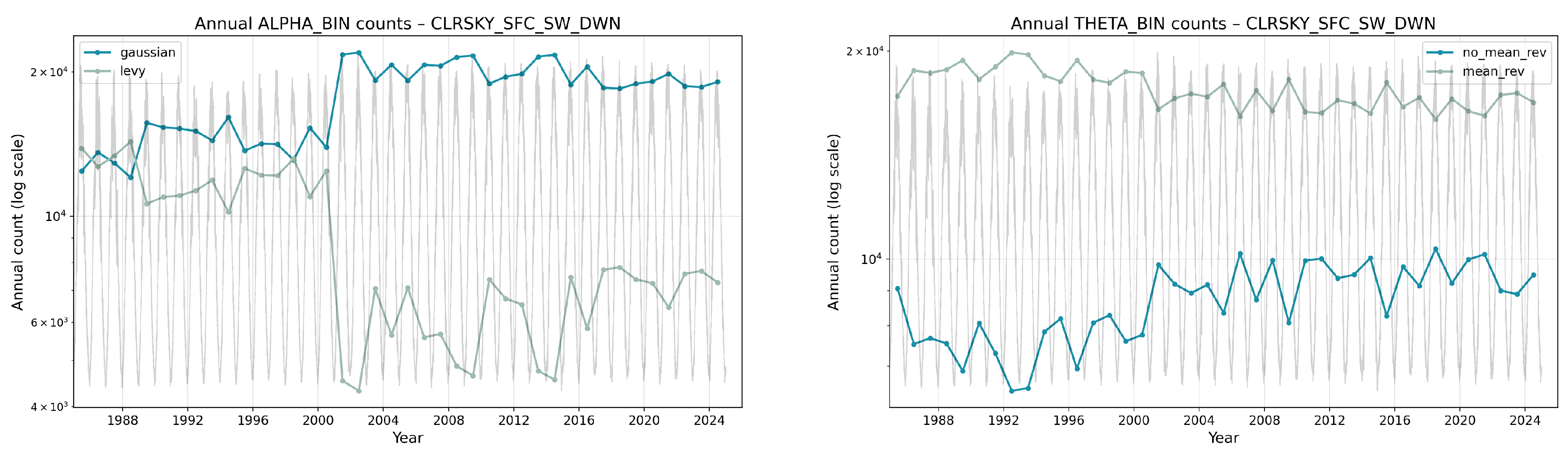
Table 4.
Absolute counts per category by period and asset.
| Period | Asset | Rows | |||||
|---|---|---|---|---|---|---|---|
| 1995–2004 | AAPL | 2297 | 1383 | 97 | 1 | 0 | 3778 |
| DJI | 2954 | 801 | 22 | 1 | 0 | 3778 | |
| GSPC | 2982 | 759 | 37 | 0 | 0 | 3778 | |
| MSFT | 2560 | 1183 | 35 | 0 | 0 | 3778 | |
| 2010–2024 | AAPL | 2325 | 1351 | 94 | 3 | 0 | 3773 |
| DJI | 2472 | 1221 | 80 | 0 | 0 | 3773 | |
| GSPC | 2451 | 1281 | 41 | 0 | 0 | 3773 | |
| MSFT | 2518 | 1226 | 29 | 0 | 0 | 3773 |
Table 5.
Absolute counts per category by period and asset.
| Period | Asset | Rows | ||||||
|---|---|---|---|---|---|---|---|---|
| 1995–2004 | AAPL | 171 | 333 | 531 | 540 | 715 | 1488 | 3778 |
| DJI | 198 | 372 | 597 | 625 | 805 | 1181 | 3778 | |
| GSPC | 202 | 386 | 599 | 592 | 805 | 1194 | 3778 | |
| MSFT | 185 | 433 | 535 | 503 | 693 | 1429 | 3778 | |
| 2010–2024 | AAPL | 116 | 354 | 534 | 575 | 833 | 1361 | 3773 |
| DJI | 139 | 397 | 595 | 600 | 809 | 1233 | 3773 | |
| GSPC | 115 | 399 | 571 | 585 | 822 | 1281 | 3773 | |
| MSFT | 196 | 487 | 536 | 543 | 766 | 1245 | 3773 |
Table 6.
Sunspots: absolute counts per distribution category by period.
| Period | Gaussian | Lévy | Observations |
|---|---|---|---|
| 1985–2004 | 4805 | 2500 | 7305 |
| 2005–2024 | 3730 | 3575 | 7305 |
Table 7.
Sunspots: absolute counts per mean-reversion category by period.
| Period | No mean reversion | Mean reversion | Observations |
|---|---|---|---|
| 1985–2004 | 2216 | 5089 | 7305 |
| 2005–2024 | 3311 | 3994 | 7305 |
Table 8.
Absolute counts per category by period and variable (all Austrian locations pooled; 50-day windows, step 1).
Table 8.
Absolute counts per category by period and variable (all Austrian locations pooled; 50-day windows, step 1).
| Period | Variable | Rows | |||||
|---|---|---|---|---|---|---|---|
| 1985–2004 | ALLSKY_SFC_SW_DWN | 252,661 | 201,027 | 69,658 | 2,605 | 9 | 525,960 |
| CLRSKY_SFC_SW_DWN | 310,660 | 194,413 | 20,817 | 40 | 30 | 525,960 | |
| PRECTOTCORR | 368 | 174,242 | 340,834 | 10,510 | 6 | 525,960 | |
| PS | 442,210 | 83,322 | 428 | 0 | 0 | 525,960 | |
| RH2M | 309,072 | 192,538 | 24,306 | 44 | 0 | 525,960 | |
| T2MDEW | 419,656 | 105,534 | 770 | 0 | 0 | 525,960 | |
| T2M_RANGE | 354,956 | 147,121 | 23,883 | 0 | 0 | 525,960 | |
| TOA_SW_DWN | 0 | 4,490 | 49,237 | 221,661 | 250,572 | 525,960 | |
| WS10M | 230,010 | 275,010 | 20,940 | 0 | 0 | 525,960 | |
| WS10M_MAX | 197,802 | 287,956 | 40,202 | 0 | 0 | 525,960 | |
| 2005–2025 | ALLSKY_SFC_SW_DWN | 267,713 | 204,414 | 53,833 | 0 | 0 | 525,960 |
| CLRSKY_SFC_SW_DWN | 395,689 | 125,553 | 4,715 | 3 | 0 | 525,960 | |
| PRECTOTCORR | 133 | 173,071 | 341,732 | 11,021 | 3 | 525,960 | |
| PS | 431,877 | 93,619 | 464 | 0 | 0 | 525,960 | |
| RH2M | 307,729 | 191,274 | 26,929 | 28 | 0 | 525,960 | |
| T2MDEW | 407,164 | 117,698 | 1,098 | 0 | 0 | 525,960 | |
| T2M_RANGE | 355,124 | 147,867 | 22,969 | 0 | 0 | 525,960 | |
| TOA_SW_DWN | 0 | 4,123 | 50,873 | 220,386 | 250,578 | 525,960 | |
| WS10M | 218,228 | 287,997 | 19,735 | 0 | 0 | 525,960 | |
| WS10M_MAX | 179,446 | 304,033 | 42,481 | 0 | 0 | 525,960 |
Table 9.
Absolute counts per category by period and variable (all Austrian locations pooled; 50-day windows, step 1).
Table 9.
Absolute counts per category by period and variable (all Austrian locations pooled; 50-day windows, step 1).
| Period | Variable | Rows | ||||||
|---|---|---|---|---|---|---|---|---|
| 1985–2004 | ALLSKY_SFC_SW_DWN | 456,012 | 37,174 | 14,292 | 6,148 | 3,456 | 8,878 | 525,960 |
| CLRSKY_SFC_SW_DWN | 90,355 | 35,795 | 40,424 | 50,499 | 150,038 | 158,849 | 525,960 | |
| PRECTOTCORR | 468,123 | 18,560 | 3,228 | 628 | 70 | 35,351 | 525,960 | |
| PS | 232,784 | 164,141 | 61,575 | 24,173 | 14,165 | 29,122 | 525,960 | |
| RH2M | 431,376 | 53,260 | 16,427 | 6,073 | 3,040 | 15,784 | 525,960 | |
| T2MDEW | 169,764 | 135,708 | 84,280 | 42,721 | 31,348 | 62,139 | 525,960 | |
| T2M_RANGE | 513,624 | 9,403 | 1,403 | 507 | 304 | 719 | 525,960 | |
| TOA_SW_DWN | 0 | 0 | 33,038 | 47,461 | 143,285 | 302,176 | 525,960 | |
| WS10M | 510,129 | 11,263 | 1,627 | 635 | 297 | 2,009 | 525,960 | |
| WS10M_MAX | 508,478 | 11,801 | 1,908 | 751 | 398 | 2,624 | 525,960 | |
| 2005–2025 | ALLSKY_SFC_SW_DWN | 434,606 | 47,345 | 18,824 | 8,867 | 5,184 | 11,134 | 525,960 |
| CLRSKY_SFC_SW_DWN | 77,316 | 30,959 | 35,538 | 50,434 | 143,284 | 188,429 | 525,960 | |
| PRECTOTCORR | 472,260 | 15,461 | 2,829 | 652 | 75 | 34,683 | 525,960 | |
| PS | 232,180 | 163,224 | 63,911 | 22,791 | 13,595 | 30,259 | 525,960 | |
| RH2M | 437,683 | 49,014 | 15,902 | 5,816 | 2,776 | 14,769 | 525,960 | |
| T2MDEW | 159,468 | 144,860 | 80,681 | 42,107 | 31,742 | 67,102 | 525,960 | |
| T2M_RANGE | 513,303 | 8,990 | 1,646 | 710 | 370 | 941 | 525,960 | |
| TOA_SW_DWN | 0 | 0 | 33,775 | 46,879 | 142,835 | 302,471 | 525,960 | |
| WS10M | 515,611 | 6,686 | 989 | 479 | 292 | 1,903 | 525,960 | |
| WS10M_MAX | 511,320 | 9,902 | 1,550 | 601 | 402 | 2,185 | 525,960 |
Disclaimer/Publisher’s Note: The statements, opinions and data contained in all publications are solely those of the individual author(s) and contributor(s) and not of MDPI and/or the editor(s). MDPI and/or the editor(s) disclaim responsibility for any injury to people or property resulting from any ideas, methods, instructions or products referred to in the content. |
© 2025 by the authors. Licensee MDPI, Basel, Switzerland. This article is an open access article distributed under the terms and conditions of the Creative Commons Attribution (CC BY) license (http://creativecommons.org/licenses/by/4.0/).
Copyright: This open access article is published under a Creative Commons CC BY 4.0 license, which permit the free download, distribution, and reuse, provided that the author and preprint are cited in any reuse.


