1. Introduction
Peatlands are crucial ecosystems that shape the terrestrial carbon balance alongside forests [
1]. Although boreal peatlands cover only 2–3% of the land surface, their peat deposits store up to 500 Gt of carbon, a stock comparable to that of forests, which occupy about 30% of the land area [
2,
3,
4]. The sequestration and long-term preservation of carbon in peatlands is crucial in regulating the climate system [
5,
6,
7]. Assessing the carbon-sink function of peatlands has been recognized internationally [
8] and nationally [
9] as a key objective for developing climate change adaptation strategies [
10]. Since 2022, Russia has been implementing the “Rhythm of Carbon” project (National System for Monitoring Carbon Pools and Greenhouse Gas Fluxes), a primary goal of which is to assess peatland carbon stocks through a developing network of permanent monitoring stations [
11].
The photosynthetic activity of the plant cover is the key process driving carbon uptake in peatland ecosystems [
12,
13], with the moss–herb–dwarf shrub layer playing the dominant role in long-term carbon storage [
14,
15]. The primary production of aboveground (AGB
1) and belowground biomass (BGB) is sustained by mosses and perennial plants (e.g., moss litter, roots, and shoots), while annual plants contribute a constant input of poorly decomposing mortmass under waterlogged conditions [
16].
However, AGB and BGB stocks in peatlands are characterized by high spatial variability, expressed through a complex microrelief
2 structure [
17,
18,
19,
20]. For instance, in patterned bogs featuring alternating ridges and hollows, AGB/BGB stocks can differ by an order of magnitude between these elements [
21,
22]. In other boreal peatland types lacking distinct ridge–hollow patterns, spatial variability driven solely by hummocks and depressions can still span severalfold [
18,
23].
The classical approach for estimating AGB/BGB stocks within specific microrelief elements is direct vegetation sampling and dry mass measurement [
24]. However, for heterogeneous peatland microrelief, this requires extensive sampling and subsequent upscaling, which depends on knowing the proportional coverage of microtopographic and microform elements across the study area [
25,
26]. Consequently, accurate spatial identification of microrelief elements is a major challenge for reliable phytomass stock assessment at the ecosystem scale [
17,
27,
28].
Satellite remote sensing is traditionally used for upscaling AGB from local to regional scales. Unfortunately, even modern systems like Sentinel-2 have a spatial resolution (10–20 m/pixel) that is too coarse to detect individual microforms; it is typically sufficient only for classifying bog landscape units (vegetation facies) and, at best, broader microtopography. Some commercial very-high-resolution sensors (0.5–2 m/pixel) could partially address the task of mapping microform areas, but they are often costly or unavailable for the target regions [
29,
30]. As an alternative, field-based visual estimation of microform coverage is a common but inherently subjective and imprecise method for upscaling phytomass stocks, identified as a significant source of uncertainty in inventories [
16,
31,
32].
In recent decades, unmanned aerial systems (UAS) equipped with LiDAR (light detection and ranging) sensors have emerged as a key tool for spatially distributed studies of peatland AGB [
33,
34,
35,
36]. UAS-LiDAR offers relatively low operational costs [
37,
38], is less dependent on cloud cover than satellite optical data [
39], and can survey terrain in remote or inaccessible areas [
40,
41,
42]. Most importantly for upscaling, LiDAR provides the best available characteristics for capturing the morphological structure of heterogeneous peatland microrelief with sub-centimeter accuracy [
43,
44]. Several studies have successfully demonstrated the potential of UAS-LiDAR for mapping peatland surface morphology on small pilot sites [
35,
45,
46]. However, there is still a lack of comprehensive, quantitative assessments comparing the results of AGB upscaling based on UAS-LiDAR-derived microtopography and microforms against traditional field-based and satellite-based estimations at matching landscape and local scales.
The aim of this study is to develop and test a simple, formalized approach for classifying bog microtopography and microforms using UAS-LiDAR data to upscale AGB/BGB stocks, and to quantitatively compare the results with traditional methods. Using a 4.64 km2 section of an ombrotrophic bog in Western Siberia as a case study, we addressed the following objectives:
To develop a straightforward formal method for classifying bog microtopography (ridges/hollows) and microforms (hummocks/depressions) from UAS-LiDAR data across different bog landscape units (vegetation facies).
To upscale field-measured AGB/BGB stocks using the resulting microtopography/microform map (LiDAR-based estimate).
To estimate phytomass stocks using two alternative methods: traditional field-based visual upscaling (field-based estimate) and classification of bog landscape units and microtopography from satellite data (satellite-based estimate).
To quantitatively compare the phytomass upscaling results from the three methods, determining their discrepancies and evaluating the importance of accounting for bog microtopography and microforms (via LiDAR) for accurate phytomass stock inventory.
2. Materials and Methods
2.1. Study Area
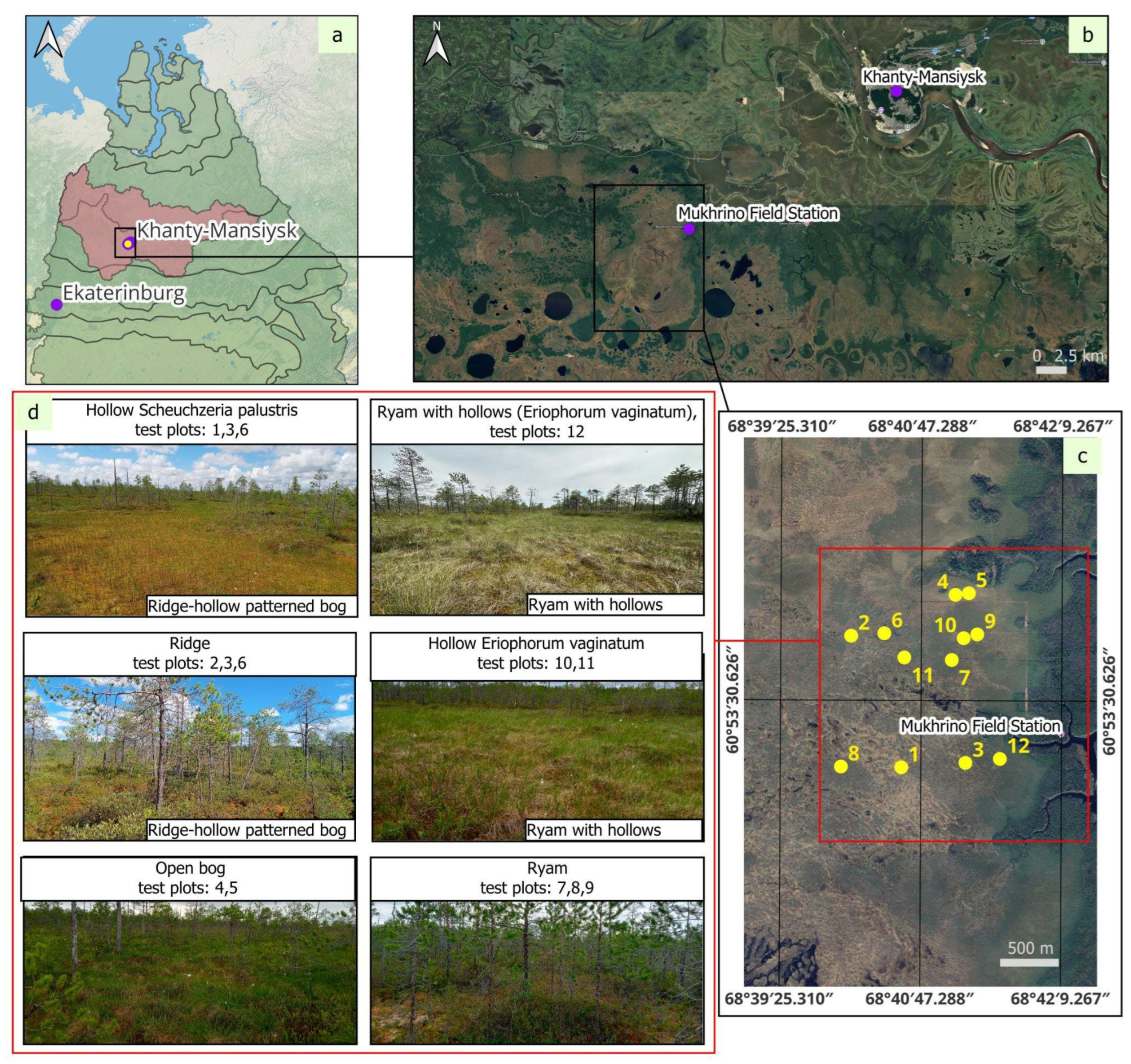
The study was conducted at the Mukhrino Field Station (MFS), located in the central part of Western Siberia within the middle taiga bioclimatic zone. The MFS is situated approximately 20 km southwest of Khanty-Mansiysk (60.892135° N, 68.682330° E), on the second terrace of the left bank of the Irtysh River, near its confluence with the Ob River. The research area occupies the northeastern part of the pristine Mukhrino mire, which covers approximately 75 km
2 (
Figure 1). To the southwest, the extensive peatland and lake landscapes of the Kondinskaya lowland are interspersed with riparian forests [
47]. The Mukhrino mire itself is an oligotrophic, raised Sphagnum bog. It occupies a local watershed between two small streams, the Mukhrina and the Bolshaya, discharging water to both.
Climate data for the region were derived from the Khanty-Mansiysk meteorological station (All-Russian Research Institute of Hydrometeorological Information – World Data Centre). For the period 1990–2024, the mean annual air temperature was −4.58 ± 3.9°C, and the mean annual precipitation was 549 ± 4.95 mm. Seasonal averages were as follows: winter (November–March) −14.1 ± 2.1°C and 32.0 ± 12.3 mm; summer (May–September) +13.0 ± 2.0°C and 61.9 ± 5.6 mm; and transitional seasons (April, October) +0.4 ± 4.1°C and 37.8 ± 7.2 mm. Maximum precipitation occurs in July, with high interannual variability (range: 7–233 mm).
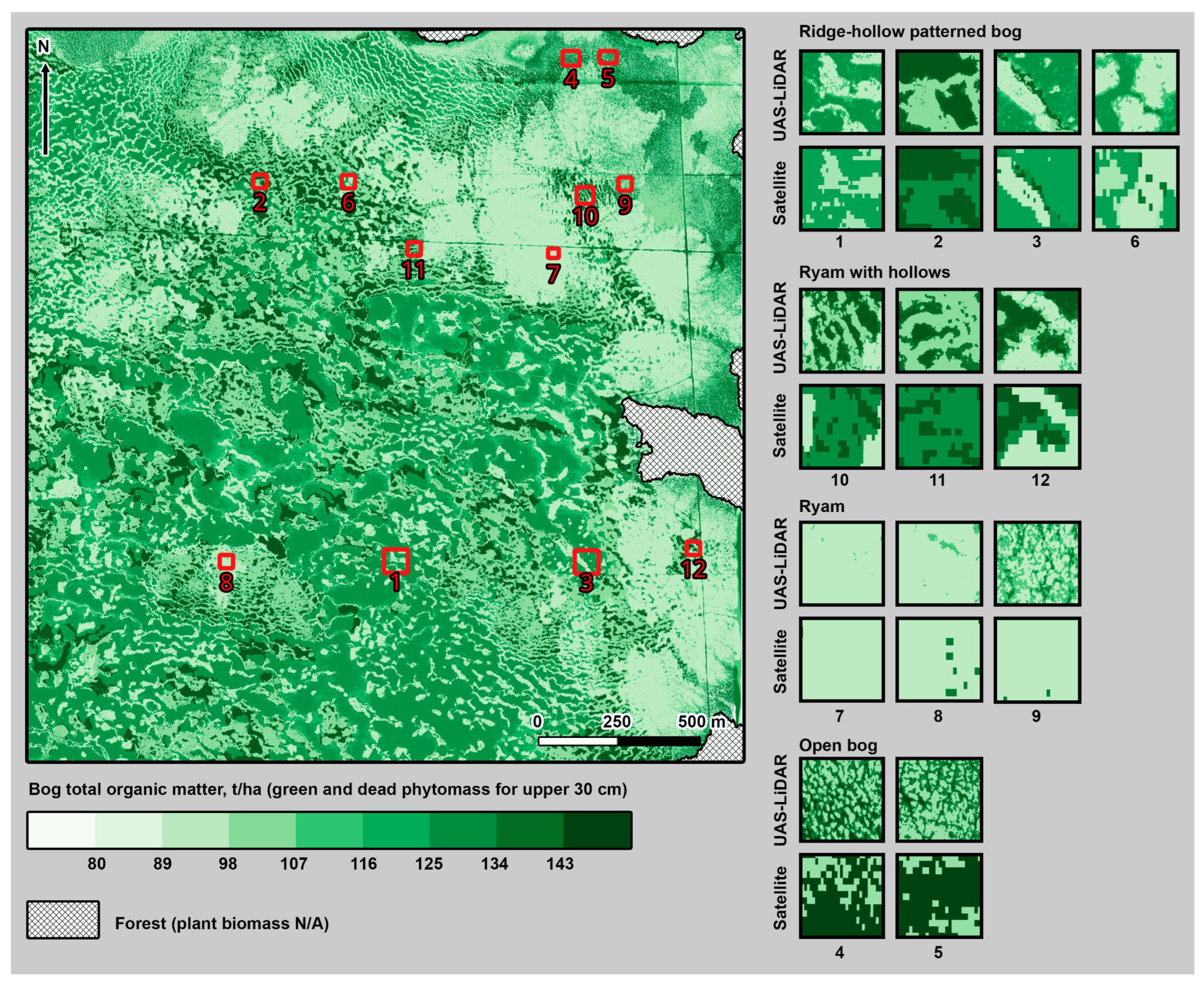
Four bog landscape units (bog types), typical of the middle taiga of Western Siberia, were investigated in this study (
Figure 1):
1. Ridge–hollow patterned bog. This is the most widespread ombrotrophic patterned bog type in Western Siberia. It consists of pine–dwarf shrub–Sphagnum ridges and Sphagnum hollows, generally oriented perpendicular to the direction of rainwater flow. The configuration and spacing of ridges and hollows are related to the slope gradient of the peatland surface. Ridges are drier and elevated 25–50 cm above the adjacent hollows. We distinguished two microtopographic elements within this unit:
- -
Ridges: Dominated by
Sphagnum fuscum with
Pinus sylvestris,
Ledum palustre, and
Chamaedaphne calyculata. Pines are typically 0.5–2.0 m tall with 3–10% cover [
49,
50]. The ridge surface features a hummocky microrelief of alternating
Sphagnum hummocks and depressions.
- -
Hollows: Represented by sedge–
Scheuchzeria–Sphagnum and cottongrass–sedge–
Sphagnum communities. The dwarf shrub layer is dominated by
Andromeda polifolia and
Vaccinium oxycoccos. The herb layer includes
Scheuchzeria palustris,
Carex limosa,
Eriophorum vaginatum, and
Drosera rotundifolia. The moss cover is dominated by
Sphagnum balticum, S.
papillosum, S.
jensenii, and S.
majus, with occasional S.
lindbergii [
49,
50]. The water table in hollows typically ranges from 0 to 15 cm below the moss surface but can rise above it during wet periods. The hollow surface also exhibits a hummocky microrelief, formed by
Eriophorum vaginatum hummocks and
Sphagnum depressions.
2. Ryam with hollows (Eriophorum vaginatum). This unit differs from the typical ryam by the presence of small hollows dominated by cottongrass–Sphagnum balticum communities. The mosaic includes Sphagnum hollows with scattered Pinus sylvestris, Ledum palustris, Chamaedaphne calyculata, and Sphagnum fuscum on hummocks, and Eriophorum vaginatum with S. balticum in depressions. The microrelief is diverse, consisting of Sphagnum and Eriophorum vaginatum hummocks alternating with small depressions.
3. Pine–dwarf shrub–Sphagnum bog (“Ryam”). This landscape unit features a well-developed but stunted tree layer (pine heights: 0.5–4 m). The dwarf shrub layer is dominated by Chamaedaphne calyculata and Ledum palustre, with Andromeda polifolia, Vaccinium uliginosum, Vaccinium oxycoccos (var. microcarpus), and Oxycoccus palustris. The herbaceous layer is represented by Rubus chamaemorus, with occasional Eriophorum vaginatum and Drosera rotundifolia. Its horizontal structure is characterized by alternating Sphagnum hummocks (average height: 30–40 cm) and depressions.
4. Sphagnum bog with sparse low pine trees (“Open bog”). This unit is characterized by Pinus sylvestris, Chamaedaphne calyculata, Eriophorum vaginatum, Sphagnum angustifolium, and S. divinum, with a very sparse or absent dwarf pine layer. It typically occurs in a 100–200 m wide transition zone between the oligotrophic raised bog and the mineral uplands, or between raised bogs and minerotrophic fens. The microforms here are represented by hummocks formed by Sphagnum and Eriophorum vaginatum, alternating with small hollows.
A detailed geobotanical description of the study areas, including plant heights, projective cover, phenophase, and vitality, is available in [
47].
2.2. Data Acquisition
2.2.1. UAS Survey
A LiDAR survey was conducted on 18 June 2023 using a Geoscan 401 Unmanned Aerial System (UAS) equipped with an AGM-MS3 LiDAR sensor (AGM Systems, Russia). The survey covered a 2.2 km (W–E) × 2.2 km (N–S) area within the Mukhrino bog massif. The geographic coordinates (WGS84) of the survey area corners were: N60.900456°, E68.655223°; N60.900495°, E68.693931°; N60.881808°, E68.694075°; N60.881734°, E68.655090°. The UAS was flown at a nadir altitude of 150 m above the bog surface, with the LiDAR transceiver oriented vertically downward (90° to the surface). This configuration yielded a point cloud with an average density of 100 points per m2.
2.2.2. Satellite Data
Multispectral satellite imagery was classified to delineate bog landscape units and estimate the proportional coverage of microtopography elements (ridges/hollows). The classification was performed on a SuperView-2 image (SpacEyes Beijing Space View Tech Co. Ltd.) acquired on 25 August 2022, with a spatial resolution of 1.68 m and spectral bands (RGB, RedEdge). The ISODATA unsupervised classification method was applied for this purpose. A detailed description of the classification and interpretation process is provided in
Section 2.3.3.
2.3. Microtopography Mapping and Classification Framework
2.3.1. Core Concept: Hierarchical Microrelief Model
The foundation of our mapping using UAS-LiDAR and upscaling approach is a hierarchical, two-level model of bog microrelief, which is central to understanding the spatial variability of AGB and BGB. This model defines two nested levels of surface structure:
Microtopography: The larger-scale element, characterized by the alternation of ridges (R) and hollows (H). Ridges are elevated, relatively well-drained linear features dominated by hummock-forming Sphagnum mosses (e.g., S. fuscum), dwarf shrubs, and stunted pines. Hollows are waterlogged depressions primarily covered by hollow-dwelling Sphagnum species (e.g., S. balticum). This level establishes the primary hydrological and vegetation gradient across the bog, with typical element dimensions ranging from ~10 to 100 meters.
-
Microforms: Finer-scale structural elements that form a mosaic within each microtopographic unit. These are hummocks (elevated patches) and depressions (waterlogged patches). Hummocks are local elevations formed by dense moss carpets or tussocks of Eriophorum vaginatum, while depressions are the wetter areas between them. This level drives small-scale heterogeneity in moisture and vegetation, with characteristic dimensions of ~0.5 to 3 meters. For analytical clarity and to reflect their hierarchical position, we use composite codes to denote each microform class:
- -
RH: Hummocks within Ridges
- -
RD: Depressions within Ridges
- -
HH: Hummocks within Hollows
- -
HD: Depressions within Hollows.
The core methodological principle involves the sequential delineation of these hierarchical levels based on a normalized elevation model (DTMnorm). First, the broad microtopography (R/H) is classified, followed by the segmentation of microforms (RH/RD and HH/HD) within each. This approach allows for the quantitative assessment of the area occupied by each microrelief element, which is critical for accurate phytomass upscaling.
2.3.2. UAS-LiDAR Data Processing and Microform Classification Algorithm
The classification of the hierarchical microrelief (microtopography and microforms) from UAS-LiDAR data was based on a normalized digital terrain model (DTMnorm) and optimized elevation thresholds. The workflow consisted of three main stages: (1) DTM generation and normalization, (2) threshold optimization, and (3) hierarchical classification.
- 1)
The raw LiDAR point cloud was processed using AGM ScanWorks (AGM Systems, Russia) and Lidar 360 (GreenValley International, USA) software. The processing chain included trajectory calculation using GNSS/IMU data (NovAtel OEM719, AGM-PS.M), point cloud alignment, error assessment based on strip discrepancies, point classification (“ground” and “low points” at 10 cm resolution), and generation of a high-resolution Digital Terrain Model (DTM). To account for the convex shape of the raised bog [
51,
52] and to create a common reference plane, a “zero surface” representing the basal level of waterlogged hollows was modeled. A point layer of 10,000 randomly distributed points was created in QGIS and populated with DTM elevation values. The highest 10% and lowest 1% of points were removed to filter outliers. A basal surface was then interpolated from the remaining points using ordinary kriging (power function variogram, SAGA GIS) and smoothed with a median filter (2000-pixel window). This basal surface was subtracted from the original DTM using the raster calculator (QGIS) to produce a normalized DTM (DTM
norm), where elevation represents height above the local bog base.
- 2)
-
The normalized DTMnorm was classified using three optimized elevation thresholds (hRH, hR и hH) that define the hierarchical structure:
- -
Microtopography level: Pixels above hRH were classified as Ridges (R), and those below as Hollows (H).
- -
Microform level within Ridges: Pixels within the Ridge class above hR were classified as Hummocks in Ridges (RH), and those below as Depressions in Ridges (RD).
- -
Microform level within Hollows: Pixels within the Hollow class above hH were classified as Hummocks in Hollows (HH), and those below as Depressions in Hollows (HD).
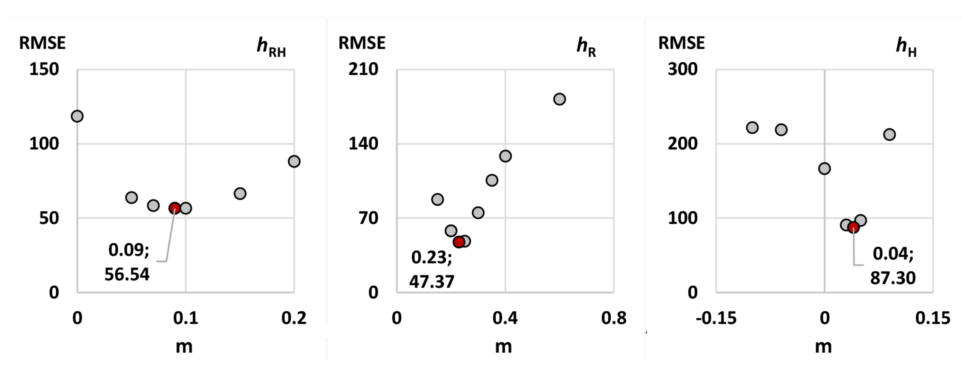
The optimal threshold values (
hRH = 0.09 m
, hR = 0.23 m,
hR and
hH = 0.04 m) were determined by minimizing the Root Mean Square Error (RMSE) between the area proportions of microforms derived from LiDAR and those from field surveys at 12 validation plots. Thresholds were tested iteratively at 1-cm intervals. The optimization results and the relationship between threshold values and RMSE are shown in
Appendix A.1. This creates a consistent elevation sequence: HD ≤
hH ≤ HH ≤
hRH ≤ RD ≤
hR ≤ RH.
- 3)
The resulting microtopography/microform map was integrated with a classified satellite image (
Section 2.3.3) to assign each microrelief element to its corresponding bog landscape unit (e.g., ridge-hollow patterned bog, ryam). Finally, the known areas of each microform within each landscape unit, combined with field-measured AGB and BGB values, were used for phytomass upscaling, as described in
Section 2.5.
2.3.3. Satellite-Based Microtopography Classification
To delineate bog landscape units and estimate the proportional coverage of microtopography elements (ridges/hollows) from satellite data, a two-stage classification was applied to the SuperView-2 multispectral image (1.68 m spatial resolution, acquired 25 August 2022; bands: RGB, RedEdge).
- 1)
Microtopography (Ridge/Hollow) Classification. Ridges and hollows were classified directly from the original image using a supervised Gaussian Maximum Likelihood classifier in Multispec software. Training data consisted of at least three verified polygons per class for the following seven spectral classes: ridges, saturated hollows, unsaturated hollows, Eriophorum hollows, open water, forest, and forest shadow. Reference accuracy for each class exceeded 97% (minimum: forest shadow), and reliability accuracy was at least 96% (minimum: Eriophorum hollows). Overall classification performance was 99% with a Kappa statistic of 0.99 (variance = 0.000009). The resulting classes were manually generalized and merged into two final microtopography classes: Ridges (R) and Hollows (H), which were then vectorized.
- 2)
Landscape Unit Classification. To identify the broader bog landscape units (vegetation types), the same SuperView-2 image was pre-processed to reduce noise and define meaningful objects. A 3×3 pixel median filter was applied eight times in GRASS GIS, followed by image segmentation with a minimum segment size of 15×15 pixels (approx. 25×25 m). For each segment, the median spectral reflectance per band was calculated, creating “superpixels”. These superpixels were classified into 10 spectral clusters using the ISODATA unsupervised method in Multispec. The clusters were then manually interpreted and generalized into the four target landscape units described in
Section 2.1: Ridge–hollow patterned bog, Ryam with hollows, Ryam and Open bog. These units were vectorized in QGIS.
Finally, the proportional area of ridges and hollows within each landscape unit polygon was calculated using zonal statistics in QGIS. The resulting landscape unit map served as a common spatial framework for all three upscaling approaches: it defined the boundaries for calculating microtopography and microform proportions from the LiDAR-based estimate, for applying field-based visual coverage ratios (field-based estimate), and for assigning satellite-derived ridge/hollow ratios (satellite-based estimate). These area ratios, together with the landscape unit map, formed the basis for the comparative phytomass upscaling as described by Formula 1 in
Section 2.5.
2.3.4. Field-Based Microlandscape Coverage Assessment
Ground-based estimation of microtopography and microform coverage was conducted through visual assessment at 12 field plots within the study area (
Figure 1,
Table 1). The classification was based on the dominant species in the tree, shrub, and herb layers, which served as the primary diagnostic criterion for distinguishing elevated (hummocks/ridges) and depressed (depressions/hollows) elements.
For landscape units with a distinct ridge–hollow structure (ridge–hollow patterned bogs and ryam with hollows), the proportional cover of both ridges/hollows and hummocks/depressions within each microtopographic element was estimated. In contrast, for the ryam and open bog units, the large-scale ridge–hollow pattern was absent or indistinguishable at the ground level. Given their relatively well-drained conditions and vegetation structure, which are more analogous to ridges in patterned bogs, these areas were treated as uniformly elevated units (“ridges”). Consequently, only the proportions of hummocks and depressions within these ridge-equivalent areas were assessed.
2.4. Phytomass Field Measurements and Fractionation
Phytomass sampling was conducted in July 2023 (peak growing season) across the 12 test plots shown in
Figure 1. Within each plot, 8 to 13 sampling sites were established to capture the variability of microforms. The sampling strategy was tailored to the landscape unit structure:
- -
In ryam and open bog units (mosaic structure), 5 sites were placed on hummocks and 3 in depressions.
- -
In ridge–hollow patterned bog and ryam with hollows units (complex ridge–hollow structure), 8 sites were located on ridges (5 on hummocks, 3 in depressions) and 5 in hollows (3 on hummocks, 2 in depressions).
At each microsite, aboveground biomass (AGB) and belowground biomass (BGB, sampled to a depth of 30 cm in 10-cm increments) were collected, separated by species and functional fraction.
AGB sampling and fractionation: Vascular plant AGB (grasses, shrubs, dwarf shrubs) was harvested by clipping within 40×40 cm quadrats. Moss AGB was collected by cutting the green, photosynthetically active parts (approximately 5 cm deep on ridges and 10 cm in hollows) using a 10×10 cm frame. AGB was separated into the following fractions: (1) green (photosynthetic) parts of vascular plants; (2) green parts of mosses and lichens; and (3) aboveground mortmass (litter, grass thatch, and standing dead shrubs).
BGB sampling and fractionation: Belowground samples were separated into: (1) live and dead roots; (2) moss litter (the non-photosynthetic layer); and (3) belowground mortmass (poorly decomposed peat with identifiable plant remains).
Laboratory processing: All samples were oven-dried at 40°C until a constant air-dry weight was achieved (3–5 days, depending on initial moisture). Weighing was performed on a balance with a precision of at least three decimal places. Oven-dry mass was calculated by dividing the air-dry mass by the hygroscopic coefficient, following standard protocols for plant biomass determination [e.g.,
53].
Field microrelief assessment: The classification of microtopography and microforms at each plot (
Section 2.3.4) was based on visual assessment, using the dominant species in the tree, shrub, and herb layers as the primary criterion for distinguishing elevated (hummocks/ridges) and depressed (depressions/hollows) elements.
2.5. Upscaling Procedures and Comparative Framework
To upscale plot-level phytomass measurements to the entire study area (4.64 km2), we developed and applied three distinct methodological pathways (LiDAR-based, Satellite-based, and Field-based), each using a different source of spatial information for area weighting. The core metric for comparison across methods is the area-weighted mean phytomass stock (Pw, in t ha−1), calculated for the entire bog using Equation 1.
For each bog landscape unit (
Section 2.1), the mean phytomass stock per unit area (t ha
−1 for AGB and BGB) was first calculated separately for each microform (RH, RD, HH, HD) using data from the corresponding field sampling sites (
Section 2.4). The area-weighted mean phytomass stock (
Pw) for the entire study bog, which represents the average stock per hectare accounting for the spatial distribution of microrelief, was then calculated as follows:
where:
Pi is the mean phytomass stock (t ha
−1) of the i-th microrelief element,
Si is the total area (ha) occupied by that element within the study area, is the total number of microrelief classes considered. The three upscaling pathways differed in the source of the area data
Si:
LiDAR-based Upscaling (Microform-level): Uses the hierarchical microtopography/microform map derived from UAS-LiDAR (
Section 2.3.2). Areas
Si correspond to the four microform classes (RH, RD, HH, HD) within each landscape unit. This approach integrates field data at the finest spatial resolution (Field microform data × LiDAR microform areas).
Satellite-based Upscaling (Microtopography-level): Uses the satellite-derived map of microtopography (
Section 2.3.3). Areas
Si correspond to the two microtopography classes (Ridges, Hollows) within each landscape unit. Field microform data were first aggregated to the microtopography level (e.g., mean stock for ridges = mean of RH and RD) before application. This represents a coarser, more traditional approach (Field microtopography data × Satellite microtopography areas).
Field-based Upscaling (Visual estimate): Uses the visually estimated proportional cover of microrelief elements from ground surveys at the 12 plots (
Section 2.3.4,
Table 1). These proportions were applied uniformly across the entire area of each corresponding landscape unit to calculate
Si. This method relies entirely on subjective field extrapolation (Field microform data × Field-visual microform areas). This comparative framework allows for a direct quantitative assessment of how the choice of spatial data (LiDAR vs. Satellite vs. Field visual) influences the final estimate of the area-weighted mean phytomass stock across the landscape.
2.6. Accuracy Assessment and Statistical Comparison
2.6.1. Accuracy of Microtopography Maps
The accuracy of the mapped microtopography and microforms was assessed using two independent approaches.
1. Error Matrix-Based Validation (Remote Sensing vs. Expert Interpretation).
The classification accuracy of the UAS-LiDAR-derived microform map (RH, RD, HH, HD) was evaluated using a standard error matrix approach. A stratified random sample of 400 validation points (100 per landscape unit) was generated across the study area. These points were not used during the threshold calibration (
Appendix A.1) and served as a fully independent validation set. An independent expert, blinded to the final LiDAR classification, visually interpreted each point by jointly analyzing the corresponding orthophoto and the high-resolution DTM, assigning it to one of the four microform classes. The expert’s reference labels were compared against the LiDAR-based map to construct an error matrix and calculate standard accuracy metrics: Overall Accuracy (OA), User’s Accuracy (UA), Producer’s Accuracy (PA), and the Kappa coefficient (κ).
The accuracy of the satellite-based microtopography map (R/H classes) was assessed using the same protocol for comparability. A new stratified random sample of 400 points (200 per class) was created. Reference labels were assigned by the same expert through a “blind” visual interpretation of the SuperView-2 multispectral image in a false-color composite (R=Infrared, G=Blue, B=Green). Results are presented in
Section 3.3.1.
Methodological Note: We acknowledge that using the same DTM for expert interpretation as for the LiDAR-based automatic classification presents a potential methodological issue, as the reference data are not fully independent of the model input. However, this approach was chosen as the most objective, as the DTM provides the most accurate and direct measurement of microrelief morphology, which is unattainable through ground surveys of random points. Crucially, the expert had no access to the results of the automated classification, ensuring the independence of their interpretation.
2. Regression-Based Comparison (Remote Sensing vs. Field Surveys).
A second validation method assessed the consistency between the area proportions of microrelief elements derived from remote sensing (both UAS-LiDAR and Satellite - based ) and those from ground surveys at the 12 validation plots (
Table 1). For each available element type, a simple linear regression was performed. The independent variable (X) was the proportional area based on ground assessment, and the dependent variable (Y) was the proportional area derived from the respective remote sensing map. This analysis was conducted for:
- -
UAS-LiDAR: hummocks and depressions within ridges (RH, RD) and hollows (HH, HD)
- -
Satellite: ridges (R) and hollows (H).
This approach quantitatively evaluated the agreement between field and remote sensing estimates of key microrelief element distributions. Results are presented in
Section 3.3.2.
2.6.2. Comparison of Phytomass Upscaling Methods
To quantitatively evaluate the differences between the upscaling methodologies, we employed a two-tier validation strategy: (1) a direct plot-scale comparison at the 12 calibration plots, and (2) an independent, landscape-scale statistical comparison of the two remote sensing-based methods.
- 1)
Plot-Scale Comparison (Calibration Plots). For each of the 12 ground calibration plots (
Table 1), the total phytomass stock (tonnes per plot) estimated by the three methods (UAS-LiDAR-based, satellite-based, and field-based) was compared. The pairwise discrepancy for each plot was quantified using two complementary metrics:
Absolute discrepancy (Δ
abs, tonnes) between two methods (
X and
Y):
where X, Y are the compared methods;
j – microtopography or microform element;
m, n – number of microtopography or microform element by method X or Y respectively;
i – plot number
Relative (symmetric) discrepancy (Δ
rel, %) between two methods (Variables defined as in Equation 2):
- 2)
-
Independent Landscape-Scale Statistical Comparison. A separate validation design provided a fully independent, statistical assessment of the two remote sensing approaches across the entire landscape:
- -
Stratified Random Sampling: We generated 100 circular validation zones, each 98.375 m2 (≈0.01 ha). To ensure representative coverage, 25 zones were randomly allocated within the mapped area of each of the four landscape units.
- -
Data Extraction and Analysis: For each zone, the total phytomass (tonnes) was extracted from both the UAS-LiDAR-based and satellite-based upscaling raster layers, creating a paired sample (n = 100). As the paired differences were not normally distributed, we used the non-parametric Wilcoxon signed-rank test (Matlab function: signrank(uas, sat)). The test evaluates the null hypothesis that the median of the paired differences (UAS − Satellite) is zero. The sign of the test statistic (stats.signedrank) was used to interpret the direction of the bias: a positive signed-rank sum indicates that the UAS-LiDAR estimates are systematically higher (satellite underestimation), while a negative sum indicates the opposite (satellite overestimation), relative to the UAS-LiDAR benchmark.
Data Extraction and Analysis: For each zone, the sum phytomass (tonnes) was extracted from the UAS-LiDAR and satellite-based raster layers, creating a paired sample (n = 100). The non-normally distributed paired differences were analyzed using the Wilcoxon signed-rank test. The test was applied in the order UAS-LiDAR estimate vs. Satellite estimate (signrank(uas, sat); Matlab), testing the null hypothesis that the median of the paired differences (UAS − Satellite) equals zero. A significant positive test statistic indicates satellite underestimation, while a significant negative statistic indicates satellite overestimation, relative to the UAS-LiDAR benchmark.
This combined validation framework enables both a detailed, plot-specific analysis of methodological discrepancies and a rigorous, independent statistical assessment of systematic biases between the primary remote sensing techniques at the landscape scale.
3. Results
3.1. Spatial Structure of Microrelief: UAS-LiDAR and Satellite-Based Assessments
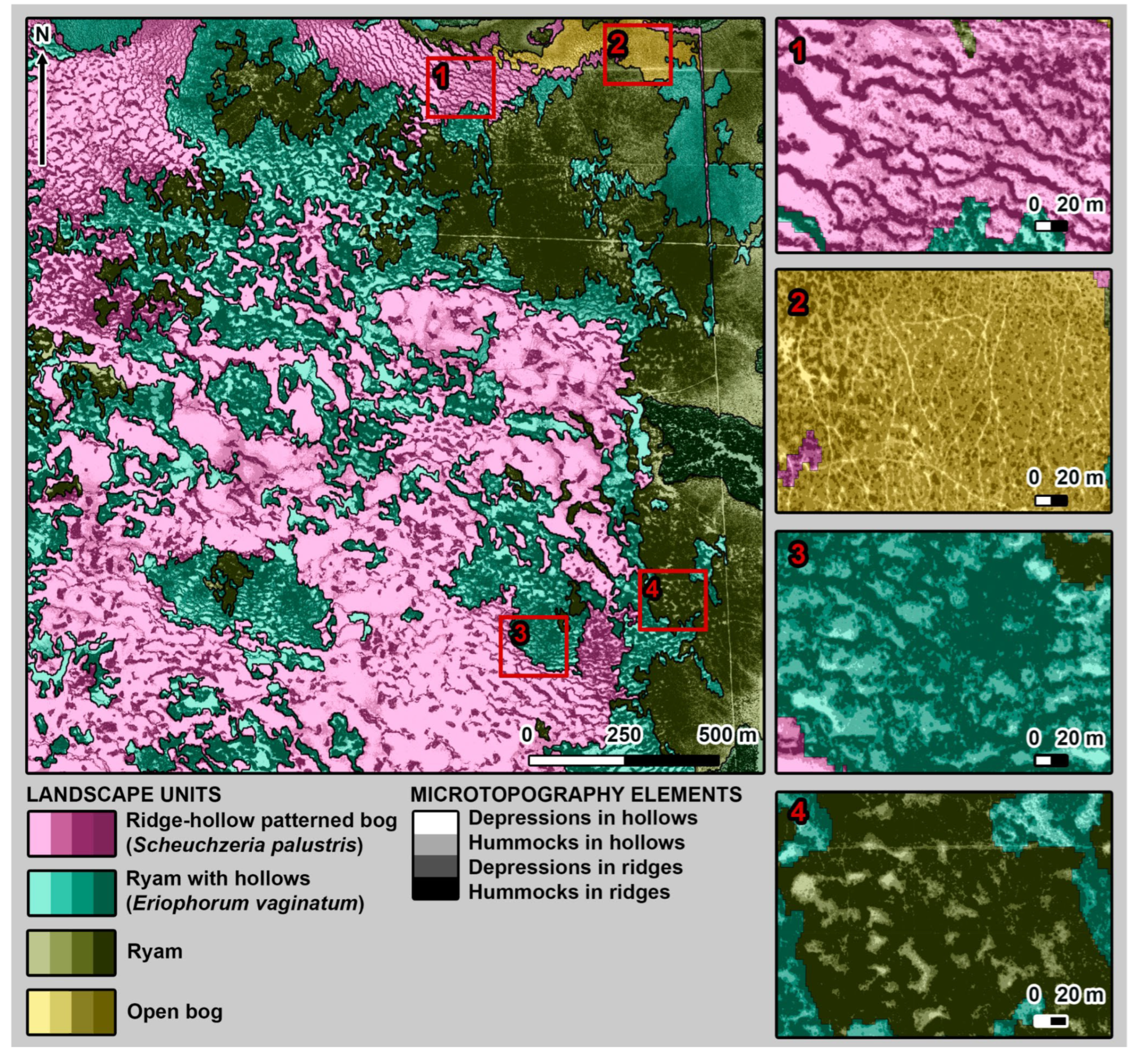
The hierarchical classification of microtopography and microforms derived from the normalized DTM (DTM
norm) is presented in
Figure 2. The map reveals the complex microrelief structure of the study bog. For the ridge–hollow patterned bog and ryam with hollows units, a clear two-level hierarchy is evident: the larger microtopography elements (ridges and hollows) contain an internal mosaic of finer microforms (hummocks and depressions). In contrast, the ryam and open bog units lack this distinct large-scale ridge–hollow pattern; their microrelief variability is expressed primarily at the level of hummocks and depressions. The total mapped area was 464 ha, with the ridge–hollow patterned bog being the most widespread unit (205 ha), followed by ryam with hollows (147 ha), ryam (107 ha), and open bog (6 ha).
The proportional coverage of microtopographic and microform elements varied substantially across the different landscape units (
Table 2). Within the ridge–hollow patterned bog, depressions (hollows) dominated, covering 66% (134 ha) of its area. Conversely, in ryam with hollows, open bog, and ryam, elevated elements (ridges) were dominant, constituting 77% (113 ha), 86% (5 ha), and 92% (98 ha) of their respective areas. Note: While classical geobotanical studies often do not distinguish ridges and hollows in ryam/open bog, treating their variability solely at the microform level, we apply a formal, elevation-based criterion relative to the bog’s basal surface, hence the classification presented here.
The surface heterogeneity of ridges, in terms of microforms, was also pronounced. The proportion of hummocks within ridges (RH) increased in the sequence: ridge–hollow patterned bog (62%) < ryam with hollows (74%) < ryam (83%). In the open bog, however, hummocks did not dominate the ridge surface (46% RH), with a larger area occupied by depressions within ridges (RD) (54%).
Hollows in all units were characterized by less contrasted microform conditions, with depressions (HD) generally prevailing. Nevertheless, the proportion of hummocks within hollows (HH) showed a concurrent increase: ridge–hollow patterned bog (24%) < ryam (35%) < ryam with hollows (36%) and open bog (59%). These data quantitatively confirm the high multi-scale spatial heterogeneity of the bog surface and provide the foundation for phytomass upscaling.
Comparison with Satellite Data. Satellite-based classification resolved the microtopography only to the level of ridges and hollows (
Table 3). The relative proportion of ridges across landscape units followed a similar trend as the LiDAR-based data: ridge–hollow patterned bog (28%) < open bog (64%) < ryam with hollows (71%) < ryam (91%).
However, the satellite-derived area of ridges was systematically lower than the LiDAR-based estimate in all units except the open bog, with differences of -6%, -6%, and -1% for the ridge–hollow bog, ryam with hollows, and ryam, respectively. A direct comparison of the total areas (
Table 2 and
Table 3) confirms that the satellite-based method consistently underestimated the proportional cover of ridges compared to the high-resolution UAS-LiDAR benchmark, highlighting a systematic bias in coarser-scale remote sensing products for microtopographic mapping.
3.2. Phytomass Stocks Across the Microtopographic Gradient
The quantification of aboveground (AGB) and belowground (BGB) biomass stocks revealed a pronounced hydro-topographic gradient, fundamentally governed by the position within the microtopographic hierarchy (landscape unit → microform). The mean stocks and their fractional composition are detailed in
Table 4.
A clear and consistent pattern emerged: the highest total organic matter stocks were found in the most waterlogged microforms—depressions within hollows (HD)—with values peaking in the Open bog (143 ± 22 t ha−1) and Ryam with hollows (131 ± 18 t ha−1). Within each landscape unit, stocks increased progressively along the wetness gradient from the most elevated and drained positions (hummocks in ridges, RH) to the most waterlogged (depressions in hollows, HD). This trend challenges the simplified assumption that elevated, drier microforms consistently support greater biomass.
The moss layer was the overwhelming driver of total phytomass, constituting 85–95% of the pool across all microsites. Crucially, the accumulation of moss mortmass was the key differentiator along the hydro-topographic gradient. Its stock increased significantly from 58 ± 1 t ha−1 on hummocks in ridges (Ridge-hollow bog) to 120 ± 3 t ha−1 in depressions in hollows (Open bog). This massive pool underscores the role of mosses not merely as primary producers but as the principal architects of long-term carbon sequestration, with accumulation driven by suppressed decomposition in waterlogged conditions, maximized in the lowest-lying depressions.
In contrast, the green biomass of mosses showed less variability (typically 12–20 t ha−1), suggesting a relatively stable productive capacity, while net accumulation (mortmass) is highly sensitive to hydro-topographic position.
The contribution of vascular plants to total AGB was minor (<15%, often <5%). Their phytomass was generally higher on ridges and hummocks (e.g., 8 ± 5 and 10 ± 5 t ha−1 in the Ridge-hollow and Open bog, respectively) than in hollows and depressions, reflecting a preference for less waterlogged conditions. The high standard deviations indicate significant small-scale patchiness. Vascular plant mortmass was negligible (<1 t ha−1), confirming their minimal contribution to the standing dead organic matter pool compared to mosses.
In summary, the spatial structure of phytomass in these boreal peatlands is defined by a strong hydro-topographic template. The total stock is predominantly built by the moss layer, with its accumulation (mortmass) maximized in the most waterlogged depressions. The vascular layer, while ecologically important, plays a secondary role in terms of overall carbon standing stock. This detailed fractional analysis is critical for understanding carbon storage drivers and for accurately scaling plot-level measurements.
3.3. Accuracy of Microtopography Mapping
3.3.1. Error Matrix Assessment
UAS-LiDAR Microform Classification. The error matrix for the UAS-LiDAR-based microform map (RH, RD, HH, HD), validated against 400 independent expert-interpreted points, is presented in
Table 5. The overall classification accuracy was 79% with a Kappa coefficient (κ) of 0.72, indicating substantial agreement according to the Landis & Koch scale.
Accuracy varied across classes. The highest User’s Accuracies were for Hummocks in ridges (RH, 86%) and Depressions in hollows (HD, 85%), indicating high reliability for these distinct endmembers. The lowest User’s Accuracy was for Depressions in ridges (RD, 70%). The main confusion occurred between RD and HH (21 points) and between HH and HD (31 points), reflecting the similarity in elevation characteristics in transitional zones between these microforms. Producer’s Accuracy was lowest for Hummocks in hollows (HH, 74%), confirming it as the most challenging class to detect accurately.
Satellite Microtopography Classification. The error matrix for the satellite-based ridge/hollow map is shown in
Table 6. The overall accuracy was 77% with a Kappa of 0.53, indicating only moderate agreement. The satellite map showed balanced but limited performance, with similar User’s (R: 78%, H: 76%) and Producer’s (R: 76%, H: 77%) accuracies for both classes, alongside substantial mutual confusion (94 misclassified points).
Direct Comparison of Methods. To enable a direct comparison at the same thematic level (ridges/hollows), the UAS-LiDAR microform map was aggregated. The resulting 2-class map achieved an overall accuracy of 95% and a Kappa of 0.89 (almost perfect agreement). User’s Accuracies were 94% (Ridges) and 96% (Hollows), and Producer’s Accuracies were 95% and 94%, respectively. In stark contrast to the satellite map (OA=77%, κ=0.53), the LiDAR data provide near-perfect discrimination of the key microtopographic elements. These results unequivocally demonstrate that UAS-LiDAR is critical for applications requiring the highest accuracy in mapping bog microrelief structures.
3.3.2. Cross-Comparison of Microtopography Mapping Methods at Test Plots
The accuracy of the microtopography and microform classifications was further assessed by comparing the proportional areas of each element derived from the UAS-LiDAR and satellite-based maps against ground survey data from the 12 validation plots using linear regression (
Table 7).
UAS-LiDAR vs. Ground. The comparison revealed strong agreement for the area of ridges (R, R2=0.7) and depressions in hollows (HD, R2=0.7), and moderate agreement for hummocks/depressions within ridges (RH/RD, R2=0.5). This demonstrates the LiDAR method’s high capability to capture key elevated elements. However, agreement was poor for hummocks within hollows (HH, R2<0.1), indicating a systematic discrepancy. This can be attributed to the inherently small and variable area HH occupies at the plot scale (0–20% ground, 0–15% LiDAR), making it highly susceptible to field estimation error or oversight. Notably, when plots without ground-identified hollows are excluded, the R2 for HH increases to 0.5 (footnote 1), underscoring the impact of field misclassification.
Satellite vs. Ground. The initial comparison showed weak performance (R2=0.2 for both R and H). However, when open bog plots (4, 5)—where both methods struggle—are excluded, agreement improves markedly (R2=0.8, footnote 2). This indicates the initial discrepancy stems not from a fundamental failure of the satellite classification, but from shared limitations of both field and satellite approaches in specific, challenging landscape units.
UAS-LiDAR vs. Satellite. A direct comparison of the two remote sensing methods showed moderate correlation when all sites were included (R2=0.5 for R/H). After excluding the problematic open bog sites, the agreement became very high (R2=0.9, footnote 2). This confirms that the UAS-LiDAR and satellite-based maps capture broad-scale microtopographic patterns congruently across most of the landscape. The key advantage of UAS-LiDAR thus lies not in mapping ridges and hollows per se, but in its superior spatial resolution, which enables the quantification of internal heterogeneity (microforms) within these larger units—a capability essential for accurate phytomass estimation.
3.4. Comparison of Phytomass Upscaling Methods
3.4.1. Landscape-Level Totals and Spatial Allocation
At the aggregate scale of the entire 4.64 km
2 study bog, the three upscaling methods yielded remarkably similar estimates of the area-weighted mean phytomass stock (
Pw): 93 ± 14 t ha
−1 (UAS-LiDAR), 95 ± 17 t ha
−1 (Satellite), and 97 ± 15 t ha
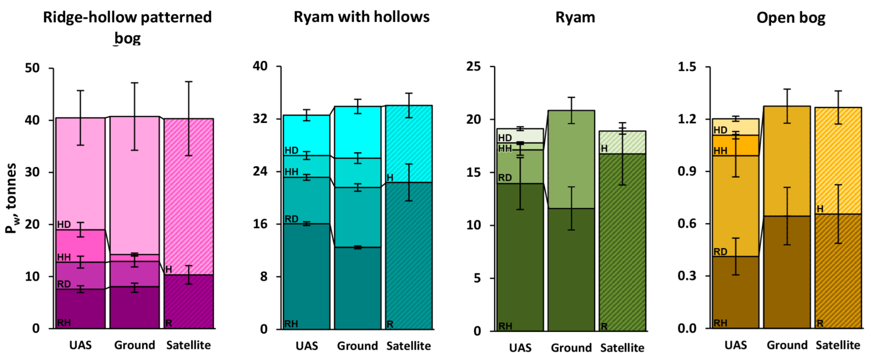
−1 (Field-based). This apparent consensus might suggest method interchangeability for large-area inventory. However, this agreement in aggregate totals masks profound and ecologically significant discrepancies in how the phytomass is spatially allocated across the microrelief hierarchy. A detailed comparison at the landscape unit level (
Figure 3) reveals critical, method-driven differences in the distribution of phytomass among microtopographic elements (ridges/hollows) and their constituent microforms (hummocks/depressions). While a formal statistical comparison across the four landscape units was not feasible (n=4), the qualitative and quantitative allocation patterns provide compelling evidence of methodological bias.
Ridge-Hollow Patterned Bog: The UAS-LiDAR approach, accounting for the full microrelief hierarchy, identified significant phytomass stocks on hummocks within hollows (HH: 6.2 ± 1.4 tonnes). This stock was nearly five times higher than the field-based estimate (1.3 ± 0.3 tonnes), which likely overlooked these small elevated features. The satellite method could not resolve HH, aggregating this stock into the broader, ecologically dissimilar “hollows” class (30.0 ± 7.1 tonnes).
Ryam with Hollows: Differences were less pronounced. The total phytomass allocated to broad ridge/hollow classes was reproducible across methods. However, the UAS-LiDAR method still revealed a more nuanced picture, showing that the field-based approach slightly underestimated phytomass on ridge hummocks (12.5 ± 0.2 vs. 16.1 ± 0.3 tonnes), highlighting the challenge of visual proportion estimation.
Ryam: The limitations of traditional methods became acute. The field method completely overlooked phytomass in hollows, misallocating it. The satellite method produced total stocks for ridges (16.8 ± 2.9 tonnes) and hollows (2.2 ± 0.3) that were comparable to the UAS-LiDAR-derived sums of their constituent microforms (17.1 ± 2.9 and 2.0 ± 0.3, respectively). However, this aggregate agreement masked its fundamental inability to reveal the internal heterogeneity (RH vs. RD) captured by LiDAR, which is critical for process-based understanding.
Open Bog: Both traditional methods failed. The field method did not detect phytomass in depressions within ridges and hummocks within hollows. The satellite method yielded similar totals but similarly failed to reflect the true spatial structure. Crucially, the satellite’s “ridges” and “hollows” in this unit corresponded, based on ground-truthing, to hummocks and depressions within ridges. This indicates that the spectral classification logic requires careful re-evaluation for non-standard landscape units like the Open bog.
In summary, while aggregate stocks were similar, the methods diverged sharply in spatially allocating phytomass to specific microforms. The UAS-LiDAR approach consistently provided the most ecologically coherent and detailed distribution, uncovering stocks missed or misaggregated by traditional methods.
3.4.2. Direct Plot-Scale Comparison of Total Phytomass at Test Plots
A direct, plot-scale quantitative comparison of the three upscaling methodologies was performed using the total phytomass estimates (tonnes per plot) for each of the 12 validation plots. The pairwise discrepancy between methods was evaluated using both the absolute discrepancy (Δ
abs, tonnes) and the relative discrepancy (Δ
rel, %) as defined in Equations 2 and 3 (
Section 2.6.2). The results for each plot are presented in
Table 8.
UAS-LiDAR vs. Satellite: Context-Dependent Agreement. For most plots (7 of 12), the two remote sensing methods showed excellent agreement (Δrel < 1%), confirming they converge on similar total stocks in landscape units where satellite microtopography classification is reliable (e.g., typical ridge-hollow bogs). However, this agreement masks critical failures. In the microform-dominated Open bog (plots 4, 5), discrepancies became extreme (Δrel = 17.9–25.8%), with satellite estimates systematically higher by 4.6–5.6 tonnes (Δabs), quantifying a severe overestimation bias where satellite resolution cannot resolve true microform structure.
UAS-LiDAR vs. Field: Plausibility and Correction of Field Errors. The comparison showed generally low-to-moderate discrepancies (Δrel = 1.7–10.9%), validating the plausibility of the LiDAR-based upscaling against traditional field extrapolation. Notably, on plot 2, a higher discrepancy (Δrel = 17.0%) suggested a local field error. Crucially, on this plot, the UAS-LiDAR and satellite estimates agreed closely (Δrel = 4.2%), while the satellite-field discrepancy was large (Δrel = 21.2%). This pattern indicates that the primary error source was the subjective field assessment, and the consistency of the two independent remote sensing methods likely reflects a more accurate representation.
In summary, while satellite-based upscaling can perform adequately in stereotypical bogs, it fails catastrophically (Δrel >25%) in heterogeneous units, introducing large systematic biases. The UAS-LiDAR method bridges this gap: it provides accuracy comparable to field methods where they are reliable, while objectively identifying and correcting substantial field errors in complex terrain, thus serving as a robust baseline for accurate phytomass distribution.
3.4.3. Independent Statistical Comparison Across the Landscape
The Wilcoxon signed-rank test applied to the paired phytomass estimates from 100 independent validation zones revealed a striking, landscape-dependent pattern of systematic bias in the satellite-based method relative to the UAS-LiDAR benchmark (
Table 9).
In the relatively homogeneous Ryam, the satellite method significantly underestimates phytomass stocks. Conversely, in the more structurally complex Ryam with hollows, the bias reverses, leading to significant overestimation. In the two most extensive units (Ridge-hollow patterned bog and Open bog), no statistically significant median bias was detected, indicating inconsistent satellite errors without a clear directional trend at the landscape scale.
This finding is critical: The error of the satellite-based method is not random noise but a predictable, systematic bias whose direction depends on the landscape context. The UAS-LiDAR approach provides the consistent reference framework needed to identify and correct these context-dependent distortions, which remain hidden when using only field-based checks or aggregate accuracy metrics.
3.4.4. High-Resolution Spatial Upscaling Based on UAS-LiDAR
Applying the validated UAS-LiDAR upscaling pathway, we generated a continuous, high-resolution (0.09 m) map of phytomass stocks for the entire study area (
Figure 4). This map spatially integrates the microtopography/microform classification (
Figure 2) with the measured phytomass gradients (
Table 4) using the area-weighting algorithm (Formula 1).
The map provides a spatially explicit representation of fine-scale heterogeneity driven by microforms. Two notable patterns emerge:
- 1)
In areas mapped as Ryam (e.g., near plot 9) and Open bog (plots 4, 5), the LiDAR-based map reveals a fine-grained mosaic of hummocks and depressions with high contrast in phytomass values. These are the same areas where traditional upscaling methods showed the largest pairwise discrepancies (
Table 8).
- 2)
The map explicitly resolves the spatial distribution and biomass contribution of specific microforms, such as hummocks of Eriophorum vaginatum within hollows (HH), which appear as high-biomass features within waterlogged areas.
This resulting phytomass map serves as a high-fidelity, spatially explicit inventory that captures the ecological structure of the bog’s microrelief. It provides the direct spatial product of the LiDAR-based upscaling approach, whose quantitative advantages over traditional methods were established in the preceding sections.
4. Discussion
4.1. Methodological Triad: Comparing Incommensurate Models of Microrelief
The core challenge of upscaling in heterogeneous environments lies not in a lack of methods, but in the fundamentally different and incommensurate principles underlying each approach. Our three-pathway framework juxtaposes models of reality with distinct origins of uncertainty, explaining their divergent outcomes not as random errors, but as systematic consequences of their design.
The field-based visual model is intrinsically qualitative and spatially implicit. It translates the observer’s mental integration of complex patterns into discrete area percentages, a process vulnerable to cognitive bias (e.g., overlooking small features) and incapable of extrapolating local proportions to a spatially variable bog dome. This explains the sporadic, high-magnitude discrepancies (e.g., omission of hollows in ryam plots,
Table 8), which reflect the method’s subjectivity and limited representativeness rather than measurement error.
The satellite-based spectral model is spatially explicit and processing-objective, but its information is constrained by fixed resolution (~1.6 m) and the physics of reflectance. Each pixel captures a spectral aggregate of all surfaces within its footprint—tree canopy, shrubs, moss patches, and water. This forces the classification to group ecologically distinct microforms (e.g., a Sphagnum depression and an Eriophorum hummock) into spectrally defined “ridge” or “hollow” classes. Its key limitation is ecological misaggregation: it maps spectral categories, not ecological units, and its signal is confounded by vegetation layers above the target moss surface [
29,
43].
The UAS-LiDAR morphometric model also provides a spatially explicit and objective output, but it senses a different property: surface geometry. By directly measuring elevation at high resolution, it captures the topographic structure controlling hydrology. Its classification is rule-based and reproducible, derived from elevation thresholds applied uniformly across the landscape. While it objectively maps form, it does not directly show ecological function—a Sphagnum hummock and a Eriophorum tussock of similar height are morphometrically equivalent.
Therefore, we do not compare one “true” map against two “false” ones. We compare three specialized models: a subjective/partial one (field), a spectrally-aggregated one (satellite), and a morphometric/structural one (LiDAR). Within this triad, the LiDAR model serves as the most viable benchmark for this study because it alone provides a reproducible, quantitative, and spatially exhaustive representation of the structural template—the microrelief—that is the primary physical driver of the ecological gradients we aim to scale. The discrepancies quantified in
Section 3.3 and
Section 3.4 are the predictable manifestations of comparing these incommensurate representations of a complex surface.
4.2. The Morphometric-Ecological Divide in Microform Classification
The foundation of our upscaling approach is the recognition that microrelief is the primary physical driver of spatial heterogeneity in peatland biomass [
2,
17,
19]. The UAS-LiDAR approach resolves the structural template with high fidelity, but it operates within a fundamental constraint: it classifies surface morphology, not ecological assemblages. This creates a morphometric-ecological divide where formal elevation rules may not align perfectly with traditional phytosociological concepts.
Our hierarchical classification is based on relative elevation above a modeled basal surface. While this objective rule cleanly separates topographic forms (e.g., a local elevation within a hollow is classified as HH), it does not guarantee ecological equivalence. For instance, a tall Eriophorum vaginatum tussock in a hollow (HH) and a low Sphagnum ridge (R) could occupy similar absolute heights, yet represent functionally distinct microsites with different plant communities, hydrology, and carbon cycle dynamics. The classification is blind to these differences; it maps the topographic opportunity space for ecological variation.
We deliberately accepted this divide to prioritize objectivity, reproducibility, and a direct link to hydrology. The elevation-based template is a conservative, unbiased representation of the primary physical gradient (moisture) governing peatland biogeochemistry. In doing so, we explicitly distinguish our product from a vegetation map. This is not a shortcoming but a conscious methodological choice that clarifies the interpretation of our results: the LiDAR-derived maps model the physical habitat structure, to which ecological properties (like phytomass) can be—and in our study, are—statistically related.
The logical next step is to bridge this divide. The objective morphometric framework we established is the ideal structural backbone for integrating complementary data on ecological function. Future work should fuse this high-resolution topographic data with coincident hyperspectral or multispectral UAS imagery. This would allow the assignment of spectral signatures (related to species composition, moss vitality, or moisture content) to specific microform classes, moving from a map of where hummocks and depressions are to a map of what they are ecologically. Our study provides the essential, reproducible geometric foundation for this integrated, next-generation mapping of peatland microhabitats.
4.3. Validation and Drivers of the Wetness-Accumulation Phytomass Gradient
Our results quantify a distinct and ecologically significant pattern for the Mukhrino bog: phytomass stocks are maximized in the most waterlogged microforms. This “wetness-accumulation” relationship highlights that in boreal Sphagnum peatlands, long-term carbon storage is often decoupled from immediate productivity and driven primarily by the preservation of organic matter.
The total phytomass stocks we measured align with the documented range for oligotrophic bogs across the West Siberian taiga [19, 24; see
Table A2]. Notably, our observation of comparable or greater biomass in hollows versus ridges is corroborated by several regional studies. For example, [
19] report stocks in oligotrophic hollows (5536–11742 g m
−2) that rival or exceed those in adjacent ridges (5924–12596 g m
−2). Similarly, data from a nearby bog show higher stocks in hollows (6332 g m
−2) than in ridges (5678 g m
−2) [
24]. This pattern, emerging within the broader spectrum of peatland variability, underscores the functional diversity of these ecosystems and cautions against the universal application of simplified biomass models based solely on moisture or vegetation facies.
Our fractional analysis directly illustrates the classic peat-forming mechanism [
54,
55] that governs carbon stocks in these ecosystems. The total phytomass pool is overwhelmingly dominated (85–95%) by the moss layer. As expected, the dead moss phytomass (mortmass) increases sharply along the wetness gradient, from ~58 t ha
−1 on ridge hummocks (RH) to ~120 t ha
−1 in hollow depressions (HD), while green moss biomass remains relatively stable (12–20 t ha
−1). This quantifies, at the microform scale, the well-established principle that long-term carbon accumulation is driven by suppressed decomposition in waterlogged anoxic conditions, not by peak productivity. The minor contribution of vascular plants (<15% of AGB, mortmass <1 t ha
−1) further confirms the central role of mosses as the principal long-term carbon sink. Thus, our data provide a quantitative, spatially explicit validation of this fundamental process within the microrelief hierarchy, forming the mechanistic basis for the observed biomass gradient.
This verified gradient has direct consequences for upscaling. Where such a hydro-topographic biomass template exists, any methodological error that misrepresents the area of wet depressions or ecologically aggregates them with drier features—as our results show both satellite and field methods do—will disproportionately distort the total stock estimate and its functional representation. Therefore, for accurate carbon accounting and for generating realistic inputs for process-based models, capturing the spatially explicit allocation of biomass according to this microtopographic template is critical. Our UAS-LiDAR approach provides the necessary structural fidelity to achieve this, whereas traditional methods introduce uncontrolled bias by oversimplifying this fundamental ecological structure.
4.4. Implications for Spatially Explicit Carbon Accounting
Our results translate into two concrete risks for peatland carbon accounting:
- -
The Illusion of Accuracy. Field and satellite methods can produce deceptively correct total stocks while severely misrepresenting their spatial distribution (
Figure 3,
Table 8). For process-based models that simulate carbon dynamics as a function of moisture and microtopography, this incorrect allocation is not a minor error—it invalidates the model’s core logic [
21,
26] by disconnecting carbon pools from their true hydrological drivers.
- -
Predictable, Uncorrectable Bias. The satellite method’s error is not random noise but a systematic, landscape-dependent bias (
Table 9). This means regional inventories will inherit a hidden, spatially variable distortion. Its magnitude remains unknown without a high-resolution benchmark, compromising the comparability of carbon stocks across different peatland types—a fundamental requirement for national reporting or carbon credit verification.
- -
Therefore, for high-stakes applications where spatial accuracy matters—baselining carbon projects, informing restoration, or initializing ecosystem models—reliance on traditional methods that cannot resolve the microform template is a critical vulnerability. Objective microrelief mapping, as demonstrated here with UAS-LiDAR, is not merely an improvement but a necessary step to escape this methodological trap and ground peatland carbon accounting in physical reality.
5. Conclusions
This study demonstrates that high-resolution UAS-LiDAR mapping of bog microrelief—differentiating both microtopography (ridges/hollows) and microforms (hummocks/depressions)—fundamentally improves the spatial accuracy of phytomass stock upscaling in a northern peatland. We applied a straightforward, reproducible hierarchical classification based on an optimized normalized digital terrain model for a 4.64 km2 ombrotrophic bog in Western Siberia. The comparative analysis with satellite-based classification and field-visual extrapolation revealed a critical limitation: while aggregate landscape-level phytomass estimates were similar (~93–97 t ha−1), traditional methods failed to capture the true fine-scale spatial allocation of biomass. They systematically missed or misaggregated key structural elements like hummocks within hollows, leading to ecologically implausible distributions. Moreover, the satellite-based method exhibited a predictable, landscape-dependent systematic bias, undetectable without a high-resolution benchmark.
The revealed spatial pattern was governed by a clear wetness–accumulation gradient, with total phytomass dominated by moss mortmass and increasing towards waterlogged depressions. This confirms that accurate carbon stock assessment requires spatially explicit weighting of field data by the true area of microform classes, a template only reliably provided by UAS-LiDAR.
Limitations and Perspectives: Our morphometric classification, while objective and hydrologically informative, maps topographic form rather than ecological function. For instance, a Sphagnum hummock and an Eriophorum tussock of similar height are conflated, representing a morphometric-ecological divide.
These constraints, however, define clear pathways for future research. The established geometric framework is an ideal backbone for integration with coincident UAS-based hyperspectral or multispectral imagery to bridge the morphometric-ecological gap, enabling species-specific or functional trait mapping within each microform class. Furthermore, the developed high-fidelity phytomass maps can serve as ground truth for calibrating and validating satellite-based biomass products or earth system models over vast peatland areas. Finally, this approach provides the essential spatial accuracy required for baseline assessments in carbon emission reduction projects (e.g., peatland restoration) and for initializing process-based models that simulate carbon dynamics as a function of microtopographic-hydrological gradients.
Author Contributions
Conceptualization, D.V.I.; methodology, D.V.I.; software, D.V.I.; validation, D.V.I.; formal analysis, D.V.I.; investigation, I.V.K., A.A.K.; resources, M.F.K.; data curation, A.V.N.; writing—original draft preparation, D.V.I., A.V.N.; writing—review and editing, D.V.I., A.V.N.; visualization, D.V.I., A.V.N.; supervision, M.V.G., A.F.S.; project administration, D.V.I.; funding acquisition, D.V.I. All authors have read and agreed to the published version of the manuscript.
Funding
This research and APC was funded by the Russian Science Foundation, grant number 25-17-20042.
Data Availability Statement
The data presented in this study are available on request from the corresponding author.
Acknowledgments
The authors extend their sincere gratitude to all participants of the field expeditions who contributed to data collection and processing. We are particularly thankful to the engineers and technical staff who provided essential boat logistics to the Mukhrino Field Station, to Artur Niyazov for his logistical support, and to Anastasia Bor, Leonid Litvinov, Sofia Rahova, Artem Kulik, Arina Bikulova, and Ruslan Run’kov for their assistance in field measurements and phytomass sampling and processing. We also thank Tatyana Zavitaeva and Valentina Batishcheva for phytomass sample processing.
Conflicts of Interest
The authors declare no conflict of interest. The funders had no role in the design of the study; in the collection, analyses, or interpretation of data; in the writing of the manuscript, or in the decision to publish the results.
Abbreviations
The following abbreviations are used in this manuscript:
| AGB |
Aboveground Biomass |
| BGB |
Belowground Biomass |
| UAS |
Unmanned Aerial System |
| LiDAR |
Light Detection and Ranging |
| DTM |
Digital Terrain Model |
| RH |
Hummocks within Ridges |
| RD |
Depressions within Ridges |
| HH |
Hummocks within Hollows |
| HD |
Depressions within Hollows |
Appendix A
Appendix A.1
Optimization of elevation thresholds for hierarchical microrelief classification. The Root Mean Square Error (RMSE) between ground-based and LiDAR-derived area estimates is plotted against candidate threshold values for: ridge/hollow separation (hRH), hummock/depression classification within ridges (hR), and within hollows (hH). Red vertical lines mark the optimal thresholds of 0.09 m, 0.23 m, and 0.04 m for hRH, hR, and hH, respectively, corresponding to the global RMSE minima.
Optimization of elevation thresholds for hierarchical microrelief classification. The Root Mean Square Error (RMSE) between ground-based and LiDAR-derived area estimates is plotted against candidate threshold values for: ridge/hollow separation (hRH), hummock/depression classification within ridges (hR), and within hollows (hH). Red vertical lines mark the optimal thresholds of 0.09 m, 0.23 m, and 0.04 m for hRH, hR, and hH, respectively, corresponding to the global RMSE minima.
Appendix A.2
Table A2.
Mean phytomass stock (±SE) and mortmass (g m−2) for oligotrophic bog ecosystems in the study region: current study data compared with literature values.
Table A2.
Mean phytomass stock (±SE) and mortmass (g m−2) for oligotrophic bog ecosystems in the study region: current study data compared with literature values.
|
Landscape unit/ Microtopography
|
Mosses |
Grasses and shrubs |
Live Biomass (Total) |
Dead Biomass |
Total
Biomass
|
Reference |
| Middle taiga (65 km east from Khanty-Mansiysk) |
| Ryam |
451 ± 87 |
|
1923 ±302 |
8766 ±832 |
10689 |
[56] |
| Northern Taiga (62°50′–63°20′N 75°00′–75°45′E) |
| Ridge |
410 ± 38 |
305 |
2064 |
6658 ± 203 |
8722 ± 239 |
[57] |
| Hollow |
351 ± 50 |
21 |
769 |
10973 ± 1950 |
11742 ± 1889 |
| Southern taiga (56°30′–57°00′N 82°30′–83°00′E) |
| Ryam |
572 ± 51 |
436 |
2292 |
5506 ± 1050 |
7798 ± 920 |
[57] |
| Ridge |
317 ± 70 |
205 |
1474 |
4450 ± 1024 |
5924 ± 1429 |
| Hollow |
420 ± 25 |
88 |
883 |
2983 ± 87 |
3866 ± 88 |
| Southern Taiga (Tomsk, Polynyanka) |
| Tall ryam |
405±632 |
|
269±390 |
|
|
[58] |
| Low ryam |
456±104 |
|
1172±415 |
|
|
| Sedge-Sphagnum fen |
433±88 |
|
980±980 |
|
|
| Ridge |
294±23 |
|
878±170 |
|
|
| Hollow |
302±18 |
|
569±76 |
|
|
| Southern Taiga (Bakcharsky district, Tomsk region) |
| Tall ryam |
285±78 |
259±126 |
1313±287 |
4239±710 |
5577±916 |
[59] |
| Low ryam |
370±88 |
265±99 |
1220±362 |
4059±606 |
5279±692 |
| Sedge-Sphagnum fen |
369±75 |
110±37 |
1035±157 |
2692±527 |
3727±584 |
| Middle taiga (Khanty-Mansiysk) / Kukushkino bog |
| Ryam |
450 |
|
2255.6 |
8766 |
11022 |
[60] |
| Ridge |
353 |
|
1861 |
8664 |
10525 |
| Hollow |
587 |
|
1608 |
8238 |
9847 |
| Middle taiga (Khanty-Mansiysk) / Oligotrophic bog “Chistoe” |
| Ridge |
310 |
|
1547 |
4131 |
5678 |
[60] |
| Hollow |
583 |
|
1388 |
4944 |
6332 |
| Ryam |
436 |
|
1529 |
6767 |
8296 |
| Middle taiga (Nizhnevartovsk)-Oligotrophic bog “Savkino” |
| Ridge |
387 ± 21 |
|
1442 |
10687 |
12129 |
[15] |
| Hollow |
528 ± 50 |
|
1239 |
8810 |
10049 |
| Ryam |
425 ± 23 |
|
1557 |
8359 |
9916 |
| Northern taiga (Noyabrsk)/Oligotrophic bog |
| Ridge |
341 ± 31 |
267 ± 25 |
1830 ± 22 |
|
|
[15] |
Notes
| 1 |
Hereafter, “AGB” and “BGB” refer specifically to the phytomass of the moss–herb–dwarf shrub layer. |
| 2 |
Hereafter, “microrelief” refers to two hierarchically linked elements: (1) microtopography – ridges (elevated, drained areas dominated by moss, herb, shrub, and tree vegetation) and hollows (depressed, waterlogged areas dominated primarily by moss vegetation) in patterned bogs, with typical dimensions of 10¹–10² m; and (2) microforms – hummocks and depressions within ridges and hollows, with characteristic dimensions of 0.5 – 3 m. |
References
- UNEP. Global Peatlands Assessment – The State of the World’s Peatlands: Evidence for Action toward the Conservation, Restoration, and Sustainable Management of Peatlands; United Nations Environment Programme: Nairobi, Kenya, 2022. [Google Scholar]
- Gorham, E. Northern Peatlands: Role in the Carbon Cycle and Probable Responses to Climatic Warming. Ecol. Appl. 1991, 1, 182–195. [Google Scholar] [CrossRef] [PubMed]
- Clymo, R.S.; Turunen, J.; Tolonen, K. Carbon Accumulation in Peatland. Oikos 1998, 81, 368–388. [Google Scholar] [CrossRef]
- Yu, Z.; Loisel, J.; Brosseau, D.P.; Beilman, D.W.; Hunt, S.J. Global Peatland Dynamics Since the Last Glacial Maximum. Geophys. Res. Lett. 2010, 37, L13401. [Google Scholar] [CrossRef]
- Moore, T.R.; Roulet, N.T.; Waddington, J.M. Uncertainty in Predicting the Effect of Climatic Change on the Carbon Cycling of Canadian Peatlands. Clim. Chang. 1998, 40, 229–245. [Google Scholar] [CrossRef]
- Lal, R. Sequestration of Atmospheric CO2 in Global Carbon Pools. Energy Environ. Sci. 2008, 1, 86–100. [Google Scholar] [CrossRef]
- Harenda, K.M.; Lamentowicz, M.; Samson, M.; Chojnicki, B.H. The Role of Peatlands and Their Carbon Storage Function in the Context of Climate Change. In Interdisciplinary Approaches for Sustainable Development Goals; Springer: Cham, Switzerland, 2017; pp. 169–187. [Google Scholar] [CrossRef]
- IPCC. Climate Change 2022: Impacts, Adaptation and Vulnerability. Contribution of Working Group II to the Sixth Assessment Report of the Intergovernmental Panel on Climate Change; Cambridge University Press: Cambridge, UK, 2022. [Google Scholar] [CrossRef]
- Decree of the President of the Russian Federation dated 4 November 2020 No. 666 “On Reducing Greenhouse Gas Emissions”. Available online: http://www.kremlin.ru/acts/bank/45990 (accessed on 13 August 2024).
- Tanneberger, F.; Schröder, C.; Hohlbein, M.; Lenschow, U.; Permien, T.; Wichmann, S.; Wichtmann, W. Climate Change Mitigation through Land Use on Rewetted Peatlands–Cross-Sectoral Spatial Planning for Paludiculture in Northeast Germany. Wetlands 2020, 40, 2309–2320. [Google Scholar] [CrossRef]
- Kurganova, I.N.; Karelin, D.V.; Kotlyakov, V.M.; Prokushkin, A.S.; Zamolodchikov, D.G.; Ivanov, A.V.; Ilyasov, D.V.; Khoroshaev, D.A.; de Gerenyu, V.O.L.; Bobrik, A.A.; et al. A Pilot National Network for Monitoring Soil Respiration in Russia: First Results and Prospects of Development. Dokl. Earth Sci. 2024, 519, 1947–1954. [Google Scholar] [CrossRef]
- Stitt, M. Rising CO2 Levels and Their Potential Significance for Carbon Flow in Photosynthetic Cells. Plant Cell Environ. 1991, 14, 741–762. [Google Scholar] [CrossRef]
- Leakey, A.D.B.; Ainsworth, E.A.; Bernacchi, C.J.; Rogers, A.; Long, S.P.; Ort, D.R. Elevated CO2 Effects on Plant Carbon, Nitrogen, and Water Relations: Six Important Lessons from FACE. J. Exp. Bot. 2009, 60, 2859–2876. [Google Scholar] [CrossRef]
- Glatzel, S.; Worrall, F.; Boothroyd, I.M.; Moody, C.S.; Clay, G.D. Comparison of the Transformation of Organic Matter Flux Through a Raised Bog and a Blanket Bog. Biogeochemistry 2024, 167, 443–459. [Google Scholar] [CrossRef]
- Kosykh, N.P.; Koronatova, N.G.; Naumova, N.B.; Titlyanova, A.A. Above- and Below-Ground Phytomass and Net Primary Production in Boreal Mire Ecosystems of Western Siberia. Wetl. Ecol. Manag. 2008, 16, 139–153. [Google Scholar] [CrossRef]
- Laine, A.M.; Bubier, J.; Riutta, T.; Nilsson, M.B.; Moore, T.R.; Vasander, H.; Tuittila, E.S. Abundance and Composition of Plant Biomass as Potential Controls for Mire Net Ecosystem CO2 Exchange. Botany 2012, 90, 63–74. [Google Scholar] [CrossRef]
- Moore, T.R.; Bubier, J.L.; Frolking, S.E.; Lafleur, P.M.; Roulet, N.T. Plant Biomass and Production and CO2 Exchange in an Ombrotrophic Bog. J. Ecol. 2002, 90, 25–36. [Google Scholar] [CrossRef]
- Nungesser, M.K. Modelling Microtopography in Boreal Peatlands: Hummocks and Hollows. Ecol. Model. 2003, 165, 175–207. [Google Scholar] [CrossRef]
- Peregon, A.; Kosykh, N.P.; Mironycheva-Tokareva, N.P.; Ciais, P.; Yamagata, Y. Estimation of Biomass and Net Primary Production (NPP) in West Siberian Boreal Ecosystems: In Situ and Remote Sensing Methods. In Novel Methods for Monitoring and Managing Land and Water Resources in Siberia; Springer: Cham, Switzerland, 2015; pp. 233–252. [Google Scholar] [CrossRef]
- Wang, M.; Wang, S.; Cao, Y.; Jiang, M.; Wang, G.; Dong, Y. The Effects of Hummock-Hollow Microtopography on Soil Organic Carbon Stocks and Soil Labile Organic Carbon Fractions in a Sedge Peatland in Changbai Mountain, China. Catena 2021, 201, 105204. [Google Scholar] [CrossRef]
- Belyea, L.R.; Clymo, R.S. Feedback Control of the Rate of Peat Formation. Proc. R. Soc. Lond. B 2001, 268, 1315–1321. [Google Scholar] [CrossRef]
- Eppinga, M.B.; Rietkerk, M.; Borren, W.; Lapshina, E.D.; Bleuten, W.; Wassen, M.J. Regular Surface Patterning of Peatlands: Confronting Theory with Field Data. Ecosystems 2008, 11, 520–536. [Google Scholar] [CrossRef]
- Lindsay, R. Peatland Classification. In The Wetland Book; Springer: Dordrecht, The Netherlands, 2018; pp. 1515–1528. [Google Scholar] [CrossRef]
- Kosykh, N.P.; Koronatova, N.G.; Mironycheva-Tokareva, N.P.; Vishnyakova, E.K.; Ivchenko, T.G.; Kurbatskaya, S.S.; Peregon, A.M. The Bogs in a Forest–Steppe Region of Western Siberia: Plant Biomass and Net Primary Production (NPP). Water 2023, 15, 3613. [Google Scholar] [CrossRef]
- Graham, J.D.; Glenn, N.F.; Spaete, L.P.; Hanson, P.J. Characterizing Peatland Microtopography Using Gradient and Microform-Based Approaches. Ecosystems 2020, 23, 1464–1480. [Google Scholar] [CrossRef]
- Graham, J.D.; Ricciuto, D.M.; Glenn, N.F.; Hanson, P.J. Incorporating Microtopography in a Land Surface Model and Quantifying the Effect on the Carbon Cycle. J. Adv. Model. Earth Syst. 2022, 14, e2021MS002721. [Google Scholar] [CrossRef]
- Strack, M.; Waddington, J.M.; Rochefort, L.; Tuittila, E.S. Response of Vegetation and Net Ecosystem Carbon Dioxide Exchange at Different Peatland Microforms Following Water Table Drawdown. J. Geophys. Res. Biogeosci 2006, 111, G02006. [Google Scholar] [CrossRef]
- Murphy, M.T.; McKinley, A.; Moore, T.R. Variations in Above- and Below-Ground Vascular Plant Biomass and Water Table on a Temperate Ombrotrophic Peatland. Botany 2009, 87, 845–853. [Google Scholar] [CrossRef]
- Lehmann, J.R.K.; Münchberger, W.; Knoth, C.; Blodau, C.; Nieberding, F.; Prinz, T.; Pancotto, V.; Kleinebecker, T. High-Resolution Classification of South Patagonian Peat Bog Microforms Reveals Potential Gaps in Up-Scaled CH4 Fluxes by Use of Unmanned Aerial System (UAS) and CIR Imagery. Remote Sens. 2016, 8, 173. [Google Scholar] [CrossRef]
- Abdelmajeed, A.Y.A.; Juszczak, R. Challenges and Limitations of Remote Sensing Applications in Northern Peatlands: Present and Future Prospects. Remote Sens. 2024, 16, 591. [Google Scholar] [CrossRef]
- Baxendale, C.L.; Ostle, N.J.; Wood, C.M.; Oakley, S.; Ward, S.E. Can Digital Image Classification Be Used as a Standardised Method for Surveying Peatland Vegetation Cover? Ecol. Indic. 2016, 68, 150–156. [Google Scholar] [CrossRef]
- Räsänen, A.; Juutinen, S.; Kalacska, M.; Aurela, M.; Heikkinen, P.; Mäenpää, K.; Virtanen, T. Peatland Leaf-Area Index and Biomass Estimation with Ultra-High Resolution Remote Sensing. GISci. Remote Sens. 2020, 57, 943–964. [Google Scholar] [CrossRef]
- Millard, K.; Richardson, M. On the Importance of Training Data Sample Selection in Random Forest Image Classification: A Case Study in Peatland Ecosystem Mapping. Remote Sens. 2015, 7, 8489–8515. [Google Scholar] [CrossRef]
- Singh, K.K.; Frazier, A.E. A Meta-Analysis and Review of Unmanned Aircraft System (UAS) Imagery for Terrestrial Applications. Int. J. Remote Sens. 2018, 39, 5078–5098. [Google Scholar] [CrossRef]
- Korpela, I.; Haapanen, R.; Korrensalo, A.; Tuittila, E.S.; Vesala, T. Fine-Resolution Mapping of Microforms of a Boreal Bog Using Aerial Images and Waveform-Recording LiDAR. Mires and Peat 2020, 26, 03. [Google Scholar] [CrossRef]
- Morgan, G.R.; Hodgson, M.E.; Wang, C.; Schill, S.R. Unmanned Aerial Remote Sensing of Coastal Vegetation: A Review. Ann. GIS 2022, 28, 385–399. [Google Scholar] [CrossRef]
- Watts, A.C.; Ambrosia, V.G.; Hinkley, E.A. Unmanned Aircraft Systems in Remote Sensing and Scientific Research: Classification and Considerations of Use. Remote Sens. 2012, 4, 1671–1692. [Google Scholar] [CrossRef]
- Whitehead, K.; Hugenholtz, C.H. Remote Sensing of the Environment with Small Unmanned Aircraft Systems (UASs), Part 1: A Review of Progress and Challenges. J. Unmanned Veh. Syst. 2014, 2, 69–85. [Google Scholar] [CrossRef]
- Hugenholtz, C.H.; Whitehead, K.; Brown, O.W.; Barchyn, T.E.; Moorman, B.J.; LeClair, A.; Riddell, K.; Hamilton, T. Geomorphological Mapping with a Small Unmanned Aircraft System (sUAS): Feature Detection and Accuracy Assessment of a Photogrammetrically-Derived Digital Terrain Model. Geomorphology 2013, 194, 16–24. [Google Scholar] [CrossRef]
- Fraser, B.T.; Congalton, R.G. Issues in Unmanned Aerial Systems (UAS) Data Collection of Complex Forest Environments. Remote Sens. 2018, 10, 908. [Google Scholar] [CrossRef]
- Banerjee, B.P.; Raval, S.; Cullen, P.J.; Singh, S.K. Mapping of Complex Vegetation Communities and Species Using UAV-LiDAR Metrics and High-Resolution Optical Data. In Proceedings of the IGARSS 2019 - 2019 IEEE International Geoscience and Remote Sensing Symposium, Yokohama, Japan, 28 July–2 August 2019; 2019; pp. 6110–6113. [Google Scholar] [CrossRef]
- Marcisz, M.; Morga, R.; Remiorz, E.; Krasoń, T.; Michalik, B.; Nalepka, P.; Kacprzak, M.; Szecówka, G. Use of Unmanned Aerial Vehicles for Water Sampling in Hard-to-Reach Water Reservoirs. Zesz. Nauk. Politech. Śląskiej Transp. 2022, 116, 211–221. [Google Scholar] [CrossRef]
- Klemas, V.V. Remote Sensing of Coastal Wetland Biomass: An Overview. J. Coast. Res. 2013, 29, 1016–1028. [Google Scholar] [CrossRef]
- Woodget, A.S.; Fyffe, C.; Carbonneau, P.E. From Manned to Unmanned Aircraft: Adapting Airborne Particle Size Mapping Methodologies to the Characteristics of sUAS and SfM. Earth Surf. Process. Landf. 2018, 43, 857–870. [Google Scholar] [CrossRef]
- Pricope, N.G.; Minei, A.; Halls, J.N.; Chen, C.; Wang, Y. UAS Hyperspatial LiDAR Data Performance in Delineation and Classification across a Gradient of Wetland Types. Drones 2022, 6, 268. [Google Scholar] [CrossRef]
- Shukla, T.; Tang, W.; Trettin, C.C.; Chen, G.; Chen, S.; Allan, C. Quantification of Microtopography in Natural Ecosystems Using Close-Range Remote Sensing. Remote Sens. 2023, 15, 2387. [Google Scholar] [CrossRef]
- Kupriianova, I.; Kaverin, A.; Filippov, I.; Ilyasov, D.; Lapshina, E.; Logunova, E.; Kulyabin, M. The Main Physical and Geographical Characteristics of the Mukhrino Field Station Area and Its Surroundings. Environ. Dyn. Glob. Clim. Chang. 2023, 13, 215–252. [Google Scholar] [CrossRef]
- Gvozdetskii, N.A.; Krivolutskii, A.E.; Makunina, A.A. Fiziko-Geograficheskoe Rajonirovanie Tyumenskoj Oblasti (Physical and Geographical Zoning of the Tyumen Region); (In Russian). Moscow State University Publishing House: Moscow, Russia, 1973; pp. 9–28. [Google Scholar]
- Cherepanov, S.K. Sosudistye Rasteniya Rossii i Sopredel’nykh Gosudarstv (Vascular Plants of Russia and Adjacent States); (In Russian). Mir i Sem’ya: Saint Petersburg, Russia, 1995. [Google Scholar]
- Ignatov, M.S.; Afonina, O.M.; Ignatova, E.A. Checklist of Mosses of East Europe and North Asia; KMK Scientific Press: Moscow, Russia, 2006. [Google Scholar]
-
Bolota Zapadnoj Sibiri – Ikh Rol’ v Biosfere (Mires of Western Siberia – Their Role in the Biosphere); (In Russian). Zemtsov, A.A., Ed.; Tomsk State University Press: Tomsk, Russia, 1998; p. 72p. [Google Scholar]
- Liss, O.L.; Abramova, L.I.; Avetov, N.A.; Berezina, N.A.; Inisheva, L.I.; Kurnishkova, T.V.; Sluka, Z.A.; Tolpysheva, T.Y.; Shvedchikova, N.K. Bolotnye Sistemy Zapadnoj Sibiri i Ikh Prirodookhrannoe Znachenie (Mire Systems of Western Siberia and Their Nature Conservation Significance); (In Russian). Grif i K: Tula, Russia, 2001. [Google Scholar]
- Allen, S.E.; Grimshaw, H.M.; Parkinson, J.A.; Quarmby, C. Chemical Analysis of Ecological Materials; Blackwell Scientific Publications: Oxford, UK, 1974; p. 565p. [Google Scholar]
- Clymo, R.S. The Limits to Peat Bog Growth. Philos. Trans. R. Soc. Lond. B 1984, 303, 605–654. [Google Scholar] [CrossRef]
- Rydin, H.; Jeglum, J.K. The Biology of Peatlands, 2nd ed.; Oxford University Press: Oxford, UK, 2013. [Google Scholar]
- Peregon, A.M.; Kosykh, N.P.; Mironycheva-Tokareva, N.P.; Vishnyakova, E.K.; Koronatova, N.G.; Stepanova, V.A.; Kurbatskaya, S.S. Production and Destruction of Plant Organic Matter in Bog Ecosystems in the South of Western Siberia. Ecol. Divers. 2024, 1, 10004. [Google Scholar] [CrossRef]
- Peregon, A.; Kosykh, N.P.; Mironycheva-Tokareva, N.P.; Ciais, P.; Yamagata, Y. Map-Based Inventory of Wetland Biomass and Net Primary Production in Western Siberia. J. Geophys. Res. Biogeosci. 2008, 113, G01007. [Google Scholar] [CrossRef]
- Golovatskaya, E.A.; Dyukarev, E.A.; Veretennikova, E.E.; Nikonova, L.G.; Smirnov, S.V. Otsenka Dinamiki Balansa Ugleroda v Bolotakh Yuzhnoy Taezhnoy Podzony Zapadnoy Sibiri (Tomskaya Oblast’) [Assessment of Carbon Balance Dynamics in Mires of the Southern Taiga Subzone of Western Siberia (Tomsk Region)]. Pochvy Okruzhayushchaya Sreda (In Russian). 2022, 5(4), 1–18. [Google Scholar] [CrossRef]
- Golovatskaya, E.A. Biologicheskaya Produktivnost’ Oligotrofnykh i Evtrofnykh Bolot Yuzhnoy Taezhnoy Podzony Zapadnoy Sibiri [Biological Productivity of Oligotrophic and Eutrophic Mires in the Southern Taiga Subzone of Western Siberia]. Zh. Sib. Fed. Univ. Biol. 2009, 2(1), 38–53. Available online: https://elib.sfu-kras.ru/handle/2311/1223.
- Kosykh, N.P.; Mironycheva-Tokareva, N.P.; Parshina, E.K. Biudzhet Khimicheskikh Elementov v Bolotnykh Ekosistemakh Sredney Taygi Zapadnoy Sibiri [Budget chemical elements in bog ecosystems middle taiga western Siberia]. Dyn. Okruzhayushchey Sredy Glob. Izmeneniya Klim. (In Russian). 2010, 1(1), 85–95. [Google Scholar] [CrossRef]
Figure 1.
Location of the study objects: (a) geographic zoning of Western Siberia (green area) according to [
48] and borders of the Khanty-Mansiysk Autonomous Okrug – Yugra (pink); (b) overview of the oligotrophic Mukhrino bog; (c) location of the test plots within the bog; (d) photographs of the studied bog sites.
Figure 2.
Map of bog landscape units (color) and microtopography with microforms (elevations in dark, depressions in light), based on UAS-LiDAR data.
Figure 2.
Map of bog landscape units (color) and microtopography with microforms (elevations in dark, depressions in light), based on UAS-LiDAR data.
Figure 3.
Weighted phytomass (Pw, tonnes) or bog landscape units (color) and microtopography with microforms (elevations in dark, depressions in light), based on UAS-LiDAR, ground and satellite data.
Figure 3.
Weighted phytomass (Pw, tonnes) or bog landscape units (color) and microtopography with microforms (elevations in dark, depressions in light), based on UAS-LiDAR, ground and satellite data.
Figure 4.
Spatial distribution of phytomass stocks in the moss-herb-dwarf shrub layer. The map is based on upscaling ground plot data using the microtopography and microform map derived from UAS-LiDAR. Values represent the total stock of aboveground and belowground (to a depth of 30 cm) phytomass. Units: tonnes per hectare (t ha−1).
Table 1.
Characteristics of the field validation plots: location, area, and ground-estimated proportional coverage of microtopographic and microform elements.
Table 1.
Characteristics of the field validation plots: location, area, and ground-estimated proportional coverage of microtopographic and microform elements.
| Landscape unit |
N |
E |
Test plot |
Area, ha |
Ridges / Hollows |
Hummocks / Depressions |
| for Ridges |
for Hollows |
Ridge-hollow patterned bog
(Scheuchzeria palustris) |
60.89695 |
68.66849 |
1 |
0.50 |
30 / 70 |
60 / 40 |
5 / 95 |
| 60.89695 |
68.67339 |
2 |
0.16 |
30 / 70 |
65 / 35 |
0 / 100 |
| 60.89661 |
68.68649 |
3 |
0.50 |
40 / 60 |
70 / 30 |
10 / 90 |
| 60.90034 |
68.68773 |
6 |
0.16 |
40 / 60 |
65 / 35 |
5 / 95 |
| Ryam with hollows (Eriophorum vaginatum) |
60.88673 |
68.67612 |
10 |
0.25 |
70 / 30 |
55 / 45 |
10 / 90 |
| 60.88673 |
68.68667 |
11 |
0.16 |
60 / 40 |
65 / 35 |
50 / 50 |
| 60.88712 |
68.69258 |
12 |
0.16 |
80 / 20 |
70 / 30 |
50 / 50 |
| Ryam |
60.89515 |
68.67705 |
7 |
0.10 |
100 / 0 |
70 / 30 |
0 / 0 |
| 60.89505 |
68.68475 |
8 |
0.10 |
100 / 0 |
70 / 30 |
0 / 0 |
| 60.88670 |
68.66674 |
9 |
0.16 |
100 / 0 |
50 / 50 |
0 / 0 |
| Open bog |
60.89692 |
68.68870 |
4 |
0.25 |
100 / 0 |
65 / 35 |
0 / 0 |
| 60.90031 |
68.68568 |
5 |
0.25 |
100 / 0 |
60 / 40 |
0 / 0 |
Table 2.
Area of microtopography and microforms, based on UAS-LiDAR data.
Table 2.
Area of microtopography and microforms, based on UAS-LiDAR data.
| Microtopography / microform |
Ridge-hollow patterned bog (Scheuchzeria palustris) |
Ryam with hollows (Eriophorum vaginatum) |
Ryam1
|
Open bog1
|
| |
area, ha / % of total |
| Total |
205 |
147 |
107 |
6 |
| Ridges |
71 / 34 |
113 / 77 |
98 / 92 |
5 / 86 |
| Hollows |
134 / 66 |
34 / 23 |
9 / 8 |
1 / 14 |
| Hummocks in ridges |
44 / 21 |
84 / 57 |
81 / 76 |
2 / 40 |
| Depressions in ridges |
27 / 13 |
29 / 20 |
16 / 15 |
3 / 46 |
| Hummocks in hollows |
32 / 16 |
12 / 8 |
3 / 3 |
<1 / 8 |
| Depressions in hollows |
103 / 50 |
22 / 15 |
6 / 5 |
<1 / 6 |
| |
% of ridges |
| Hummocks / Depressions |
62 / 38 |
74 / 26 |
83 / 17 |
46 / 54 |
| |
% of hollows |
| Hummocks / Depressions |
24 / 76 |
36 / 64 |
35 / 65 |
59 / 41 |
Table 3.
Area of microtopography and microforms, based on satellite data.
Table 3.
Area of microtopography and microforms, based on satellite data.
| Microtopography / microform |
Ridge-hollow patterned bog (Scheuchzeria palustris) |
Ryam with hollows (Eriophorum vaginatum) |
Ryam1
|
Open1bog
|
| |
area, ha / % of total |
| Total |
205 |
147 |
107 |
6 |
| Ridges |
57 / 28 |
105 / 71 |
97 / 91 |
4 / 64 |
| Hollows |
148 / 72 |
42 / 29 |
9 / 9 |
2 / 36 |
Table 4.
Specific phytomass of the moss–herb–dwarf shrub layer (mean ± σ, t ha−1) across microtopographic and microform elements for the four bog landscape units. Values are separated into organic matter fractions.
Table 4.
Specific phytomass of the moss–herb–dwarf shrub layer (mean ± σ, t ha−1) across microtopographic and microform elements for the four bog landscape units. Values are separated into organic matter fractions.
| Microtopography / microform |
Ridge-hollow patterned bog (Scheuchzeria palustris) |
Ryam with hollows (Eriophorum vaginatum) |
Ryam1
|
Open bog1
|
| |
Total organic matter, tonnes per ha ± σ |
| Hummocks in ridges (RH) |
80 ± 7 |
89 ± 2 |
80 ± 14 |
87 ± 22 |
| Depressions in ridges (RD) |
90 ± 20 |
112 ± 7 |
90 ± 14 |
106 ± 22 |
| Hummocks in hollows (HH) |
91 ± 20 |
128 ± 23 |
100 ± 14 |
124 ± 22 |
| Depressions in hollows (HD) |
97 ± 24 |
131 ± 18 |
110 ± 15 |
143 ± 22 |
| |
Moss dead phytomass, tonnes per ha ± σ |
| Hummocks in ridges (RH) |
58 ± 1 |
61 ± 1 |
59 ± 1 |
71 ± 2 |
| Depressions in ridges (RD) |
75 ± 2 |
85 ± 1 |
70 ± 1 |
87 ± 2 |
| Hummocks in hollows (HH) |
74 ± 2 |
103 ± 2 |
80 ± 1 |
103 ± 2 |
| Depressions in hollows (HD) |
82 ± 2 |
111 ± 2 |
90 ± 2 |
120 ± 3 |
| |
Moss green phytomass, tonnes per ha ± σ |
| Hummocks in ridges (RH) |
14 ± 1 |
19 ± 1 |
13 ± 1 |
7 ± 1 |
| Depressions in ridges (RD) |
10 ± 1 |
20 ± 1 |
14 ± 1 |
11 ± 1 |
| Hummocks in hollows (HH) |
12 ± 1 |
16 ± 1 |
15 ± 1 |
14 ± 1 |
| Depressions in hollows (HD) |
12 ± 1 |
16 ± 1 |
16 ± 1 |
18 ± 1 |
| |
Vascular plants phytomass1, tonnes per ha ± σ |
| Hummocks in ridges (RH) |
8 ± 5 |
9 ± 2 |
7 ± 5 |
10 ± 5 |
| Depressions in ridges (RD) |
4 ± 3 |
7 ± 2 |
7 ± 5 |
8 ± 5 |
| Hummocks in hollows (HH) |
4 ± 3 |
9 ± 2 |
5 ± 5 |
7 ± 4 |
| Depressions in hollows (HD) |
4 ± 2 |
4 ± 3 |
4 ± 3 |
5 ± 4 |
| |
Vascular plants mortmass, tonnes per ha ± σ |
| Hummocks in ridges (RH) |
0.5 ± 0.3 |
0.4 ± 0.3 |
0.4 ± 0.4 |
0.8 ± 0.7 |
| Depressions in ridges (RD) |
0.4 ± 0.4 |
0.4 ± 0.4 |
0.4 ± 0.3 |
0.6 ± 0.5 |
| Hummocks in hollows (HH) |
0.3 ± 0.3 |
0.5 ± 0.2 |
0.3 ± 0.3 |
0.5 ± 0.5 |
| Depressions in hollows (HD) |
<0.1 ± 0.1 |
0.2 ± 0.2 |
0.2 ± 0.1 |
0.3 ± 0.3 |
Table 5.
Error matrix and accuracy assessment for the microtopography classification based on UAS-LiDAR data.
Table 5.
Error matrix and accuracy assessment for the microtopography classification based on UAS-LiDAR data.
| Reference Data |
Map Data |
N |
PA, % |
| RH |
RD |
HH |
HD |
| Hummocks in ridges (RH) |
86 |
17 |
0 |
1 |
104 |
83 |
| Depressions in ridges (RD) |
14 |
70 |
8 |
0 |
92 |
76 |
| Hummocks in hollows (HH) |
0 |
13 |
75 |
14 |
102 |
74 |
| Depressions in hollows (HD) |
0 |
0 |
17 |
85 |
102 |
83 |
| N |
100 |
100 |
100 |
100 |
400 |
|
| UA,% |
86 |
70 |
75 |
85 |
|
|
Table 6.
Error matrix and accuracy assessment for the microtopography classification based on satellite data.
Table 6.
Error matrix and accuracy assessment for the microtopography classification based on satellite data.
| Reference Data |
Map Data |
N |
PA, % |
| R |
H |
| Ridges (R) |
155 |
49 |
204 |
76 |
| Hollows (H) |
45 |
151 |
196 |
77 |
| N |
200 |
200 |
400 |
|
| UA,% |
78 |
76 |
|
|
Table 7.
Coefficients of determination (R2) from linear regressions comparing the proportional area of microrelief elements derived from UAS-LiDAR, satellite, and ground-based methods across 12 test plots.
Table 7.
Coefficients of determination (R2) from linear regressions comparing the proportional area of microrelief elements derived from UAS-LiDAR, satellite, and ground-based methods across 12 test plots.
| |
UAS-Ground |
Sat.-Ground |
UAS-Sat. |
| R |
H |
RH |
RD |
HH |
HD |
R |
H |
R |
H |
| R2 |
0.7 |
0.7 |
0.5 |
0.5 |
<0.1 |
0.7 |
0.2 |
0.2 |
0.5 |
0.5 |
| |
|
|
|
0.51
|
|
0.82
|
0.82
|
0.92
|
0.92
|
Table 8.
Total phytomass stock estimates (tonnes per plot) from the three upscaling methods and their pairwise relative (Δrel, %) and absolute (Δabs, tonnes) discrepancies for the 12 validation plots.
Table 8.
Total phytomass stock estimates (tonnes per plot) from the three upscaling methods and their pairwise relative (Δrel, %) and absolute (Δabs, tonnes) discrepancies for the 12 validation plots.
| Landscape unit |
Test plot |
Total Phytomass (tonnes) |
Δrel, % / Δabs, tonnes |
| UAS |
Satellite |
Ground |
UAS-Sat. |
UAS-Ground |
Sat.-Ground |
Ridge-hollow patterned bog
(Scheuchzeria palustris) |
1 |
46.1 |
46.1 |
46.9 |
0.2 / 0.1 |
1.7 / 0.8 |
1.9 / 0.9 |
| 2 |
18.1 |
18.8 |
15.2 |
4.2 / 0.8 |
17.0 / 2.8 |
21.2 / 3.6 |
| 3 |
47.0 |
46.9 |
45.9 |
0.2 / 0.1 |
2.3 / 1.1 |
2.0 / 0.9 |
| 6 |
14.1 |
14.1 |
14.8 |
0.1 / <0.1 |
5.0 / 0.7 |
5.0 / 0.7 |
| Ryam with hollows (Eriophorum vaginatum) |
10 |
25.4 |
25.2 |
27.3 |
1.0 / 0.2 |
7.2 / 1.9 |
8.2 / 2.1 |
| 11 |
15.9 |
17.0 |
17.6 |
7.0 / 1.2 |
10.3 / 1.7 |
3.3 / 0.6 |
| 12 |
16.3 |
16.2 |
16.6 |
0.7 / 0.1 |
1.7 / 0.3 |
2.4 / 0.4 |
| Ryam |
7 |
7.3 |
7.3 |
7.6 |
0.1 / <0.1 |
3.6 / 0.3 |
3.5 / 0.3 |
| 8 |
12.9 |
13.0 |
13.2 |
1.0 / 0.1 |
2.7 / 0.4 |
1.7 / 0.2 |
| 9 |
14.2 |
13.0 |
13.7 |
8.9 / 1.2 |
3.0 / 0.4 |
5.8 / 0.8 |
| Open bog |
4 |
23.4 |
27.9 |
20.9 |
17.9 / 4.6 |
10.9 / 2.4 |
28.6 / 7.0 |
| 5 |
18.9 |
24.5 |
17.9 |
25.8 / 5.6 |
5.5 / 1.0 |
31.1 / 6.6 |
| Mean |
|
|
|
|
5.6 / 1.2 |
5.9 / 1.1 |
9.6 / 2.0 |
Table 9.
Results of the Wilcoxon signed-rank test comparing Satellite-based and UAS-LiDAR total phytomass estimates across landscape units.
Table 9.
Results of the Wilcoxon signed-rank test comparing Satellite-based and UAS-LiDAR total phytomass estimates across landscape units.
| Landscape unit |
p-value |
Significant (α=0.05) |
z-value |
Interpretation (Satellite relative to UAS-LiDAR) |
| Ridge-hollow patterned bog |
0.83 |
– |
–0.2 |
No significant bias |
| Ryam with hollows |
0.01 |
+ |
–2.8 |
Significant OVERESTIMATION |
| Ryam |
0.01 |
+ |
2.7 |
Significant UNDERESTIMATION |
| Open bog |
0.16 |
– |
–1.4 |
No significant bias |
|
Disclaimer/Publisher’s Note: The statements, opinions and data contained in all publications are solely those of the individual author(s) and contributor(s) and not of MDPI and/or the editor(s). MDPI and/or the editor(s) disclaim responsibility for any injury to people or property resulting from any ideas, methods, instructions or products referred to in the content. |
© 2025 by the authors. Licensee MDPI, Basel, Switzerland. This article is an open access article distributed under the terms and conditions of the Creative Commons Attribution (CC BY) license (http://creativecommons.org/licenses/by/4.0/).