
Submitted:
08 December 2025
Posted:
09 December 2025
You are already at the latest version
Abstract
Modern industrial equipment is a cyber-physical system (CPS) consisting of physical production components and digital controls. Lowering maintenance costs and increasing availability is important to improve its efficiency. Modern methods, based on solving event prediction problem, in particular, prediction of remaining useful life (RUL) are used as a crucial step in a framework of the reliability-centered maintenance to increase efficiency. But modern methods of RUL forecasting fall short when dealing with real-world scenarios, where CPS are described by multidimensional continuous high frequency data with working cycles with variable duration. To overcome this problem, we propose a new method for faults prediction, which is based on extraction of semantic state vectors (SSV) from working cycles of equipment. To implement SSV extraction, a new method, based on convolutional autoencoder and extraction of hidden state is proposed. In this method, working cycles are detected in input data stream, then they are converted to images, on which autoencoder is trained. The output of an intermediate layer of autoencoder is extracted and processed into SSV. SSVs are then combined into a time series, on which RUL is forecasted. After optimization of hyperparameters the proposed method shows following results: RMSE = 1.799, MAE = 1,374, which is significantly more accurate than existing methods. Therefore, SSV extraction is a viable technique for forecasting RUL.
Keywords:
cyber-physical systems
; prognosis and predictive health management
; semantic state vectors
; remaining useful life forecasting
; convolutional autoencoder
; deep learning
1. Introduction
Modern energy facilities and advanced manufacturing plants are essentially cyber-physical systems (CPS), integrating physical production components with digital control mechanisms to ensure efficient and timely production [1,2]. Here, we focus on diverse cyber-physical systems in the energy domain, notably those in power generation, which include turbines, generators, and automatic control systems featuring data collection and control elements. Typically, the digital component of CPS consists of sensors, actuators, software applications, and networking components that operate in real-time mode [3]. The implementation of such systems can substantially enhance production efficiency and elevate product quality while also reducing costs. As such, the operation of CPS has a profound impact on the competitive edge and operational efficiency of manufacturing companies [4].
The performance of CPS depends on their reliability, particularly their ability to consistently perform intended functions or maintain availability of both physical and digital components [5]. Reliability management is a complex problem that requires comprehensive data collection and analysis, as well as decision making support to address technical impacts or control actions on an equipment. This problem is amplified by the unique nature of CPS, which is expressed on the limits of such cyber-physical systems.
- Industrial energy CPSs are characterized by continuous high frequency data collected by multiple sensors (multidimensional continuous high frequency data, pMCHF).
- The operation of cyber-physical systems involves working cycles of varying duration, necessitating specific processing of the input data (cycles’ time variation, pCTV).
Basically, there are approaches to maintenance within the framework of the reliability management process: corrective maintenance, preventive maintenance and reliability-centered maintenance. Currently, the most promising concept is called prognosis and predictive health management (PPHM) and might be considered the next generation of a reliability-centered maintenance approach. PPHM is considered a very promising approach in Industry 4.0 despite current challenges and limitations [6].
PPHM is based on the idea of a threefold approach: (i) gathering data (an observe stage), (ii) assessing and predicting the technical condition of a cyber-physical system, and predicting its remaining useful life and predicting potential failures (an analyze stage) and (iii) making and executing decisions (or act stage) [7]. The second stage includes the prediction problem, which can be decomposed into the following task: forecast the health indicator (or health index) for a certain horizon, estimate remaining useful life (RUL) and predict the faults (FP). Decisions initiate practical activities such as inspection, maintenance, and system configuration, all aimed at optimizing system performance and longevity [8].
Based on formalization [9], consider a set O of cyber-physical systems of the same type . Each system is equipped with a range of sensors S to gather data on the performance of its components. Each sensor captures a set of measurements over a given observation period T. These sets are formed into a matrix of observations or dataset D. For given cyber-physical systems O, there may be numerous incident reports E containing information about timestamps of failure events and transition to the limiting state as a set of pairs . So, it is needed to find the model
where is the model’s output, and is a loss function, and A is a finite set of models (algorithms).
Given a new cyber-physical system of the same type , which has the same set of sensors and its own dataset of observations , it is needed to determine the time at which failure or/and end of life occurs using .
Within this framework, two types of events are considered: the failure event and the transition to a limiting state or the end of life event. For the first type of event, the problem of Failure Prediction, or FP-problem, is considered, as well as for the second type, the remaining useful lifetime prediction, or RUL-problem. Formally, both FP-problem and RUL-problem can be generalized as the prediction of the time at which a specific event occurs, or Event Prediction problem, EP-problem. Consequently, the EP-problem can be effectively formulated as regression problems, where the aim is to predict the time until the occurrence of these critical events [10,11].
The EP-problem is a well-known problem in the field of machinery and reliability management [12]. However, it is necessary to point out the following open question related to the mentioned above limitation of the CPS. Most published solutions of the EP-problem for complex equipment utilize well known datasets, like the TurboFan [13], which contains aggregated data over the working cycles. Models that have proven themselves well in solving show very limited results when applied to high-frequency data. It means, it is necessary to find novel approaches to data preprocessing or to develop new forecasting models. Efforts to address the challenge of EP-problem without preprocessing have yielded unsatisfactory outcomes. Also, this is due to the fact that there are significant variations in the working cycle durations in other datasets. To address this issue, it is necessary to develop models with adaptive input layers that can accommodate such variability. As a result, even the most advanced techniques may demonstrate substantial inaccuracies when directly applied to this particular dataset [14].
Typically, there are three main groups of EP-problem approaches: physics bases (model-based), data-driven (machine learning, statistical learning), and hybrid [7]. Model-based approaches typically involve the development of mathematical models that serve as representations of the physical properties of a system and its potential modes of failure. One significant challenge lies in the difficulty of adapting models in real time to accommodate dynamic changes within the system. Furthermore, model-based methodologies cannot be employed for intricate systems whose internal variables are either difficult or impossible to measure directly using sensors. In contrast, data-driven methods employ the analysis of collected data to identify and establish patterns that can be utilized to forecast the remaining useful life of new data sets.
In this context, an issue arises – the development of a method for RUL estimation of cyber-physical systems that are characterized by multi-dimensional and instantaneous measurements or have all above-mentioned limitations. The idea of the contributed method is to analyze the convolutional layers and extract hidden states from the convolutional architecture, transforming these states into a semantic state vector that encapsulates the state of the system throughout its operational cycle. It means, the proposed method for solving EP-problem in CPS based on the extraction of a semantic state vector (SSV) can be understood through recent advances in semantic-functional communication and state representation within CPS.
2. Background
This section surveys recent academic works addressing EP-problems for the limitations determined above, specifically focusing on intelligent fault diagnosis and RUL prediction mainly for rotating machinery like bearings and milling tools. The review is structured into two main parts:
- Innovative Model Architectures. The first part covers papers which propose novel deep-learning model structures to improve diagnostic accuracy and prediction.
- Advanced Data Preprocessing & Representation. The second part highlights papers that focus on transforming raw, high-frequency sensor data (like vibration and acoustic signals) into more informative formats, primarily 2D time-frequency images, to enhance model performance.
2.1. Innovative Model Architectures
The opening series of papers examines innovative model architectures designed to solve core predictive maintenance tasks: estimating remaining useful life and forecasting failures for intelligent fault diagnosis. All papers provide results that improve performance indicators for datasets consisting of of high frequency data, like XJTU–SY [15] or NASA Bearing Dataset [16].
The idea of an ensemble of deep learning models for intelligent fault diagnosis is proposed by J. Niyongabo et al. [17]. Particularly, authors propose a fault diagnosis model for rolling bearings based on an ensemble of networks, combining improved DenseNet and SENet models.
Another idea is presented by J. Yu and H. Hu [18] where wide convolutional kernels are used for initial feature extraction. As a novel result, this paper proposes a Multi-Scale Convolutional Neural Network with Self-Knowledge Distillation (MSCNN-SKD) for bearing fault diagnosis.
W. Gong et al. [19] suggest applying support vector machine (SVM) method and global average pooling technology to enhance the structure of CNN for fault classification.
S. Xiong et al. [20] propose a novel network named WPT-CNN (from Wavelet Packet Transform into Convolutional Neural Network Structures) for an end-to-end intelligent fault diagnosis of rolling bearings. The main idea is to fuse time-frequency analysis ability into the architecture of the classification model and automatically search for more suitable time-frequency coefficients during the training process.
Another interesting architecture with high-performance double pyramidal fusion module, or HDPF is presented by X. Zhao et al. in a paper [21]. This module allows the extraction of more adequate and effective multiscale complex feature information.
X. Li et al. [22] propose a novel multi-branch feature cross-fusion bearing fault diagnosis model (MCFormer). The core of the paper is a multi-branch structure extracting local features from each sensor separately.
M. Sohaib et al. [23] suggest another hybrid feature pool that is used in combination with sparse stacked autoencoder (SAE)-based deep neural networks (DNNs) to perform an effective diagnosis of bearing faults of multiple severities. The fusion model provides more accurate and reliable RUL predictions than models using only a single data source, highlighting the benefit of multimodal high-frequency data integration.
A bearing fault diagnosis method based on mixed pooling deep belief network (MP-DBN) is suggested by J. Tang et al. [24]. Adopted Morlet wavelet is used to obtain the corresponding time–frequency representation.
Another interesting model based on the domain-adversarial neural network (DANN) and attention mechanism to identify rolling bearing faults is proposed by H. Wu et al. [25]. The authors claim that the feature extractor with an attention mechanism enables the model to learn and retain key features related to the faults during the training process.
H. Wang et al. [26] improve the sparrow search algorithm (ISSA) for configurable parameters in the Long Short-Term Memory (LSTM) network for RUL prediction. The experimental dataset featuring LDK UER204 rolling element bearings from the XJTU–SY bearing was used [15]. It is shown, that RMSE of the prediction is quite small (RMSE = 0.007).
2.2. Advanced Data Preprocessing & Representation
The next part of the review includes articles on EP-problems that propose original solutions for data preprocessing, including transformation into another representation.
The time–frequency domain (TFD) features such as short-time Fourier-transform (STFT) and different wavelet transforms (WT) are considered as preprocessing techniques for the RUL estimation of the milling cutter by S. Sayyad et al. [27]. The TFD feature extraction technique has been shown to be effective for RUL prediction with deep learning models such as LSTM, CNN, and hybrid CNN model with LSTM variants. The IEEE NUAA Ideahouse dataset was used in the paper.
I. Makrouf et al. presented a novel [28] multi-sensor fusion approach for bearing fault diagnosis that combines vibration and acoustic signals within a transfer learning framework. Continuous Wavelet Transform (CWT) is applied to multi-sensor inputs, and the resulting wavelet coefficients are fused using the Maximum Energy to Shannon Entropy Ratio (ME-to-SER) criterion to fine-tune pre-trained Convolutional Neural Networks (CNNs).
Interesting research regarding the search for an optimal (minimal) input vector is presented by J. Chen et al. [29]. In the work, the low bound for input size of 2D data is analyzed by considering the relationship between the characteristic vibration frequencies and the window size of short-time Fourier transform (STFT) to guide the determination of the minimum input size. CNN is also used as the main architecture of the model.
The idea of extracting features from multiple sensor data is presented in a paper by M. Liu et al. [30]. Authors use feature extraction and generation approaches, e.g. analyzing features in time domain (TD), frequency domain (FD) and time-frequency domain (TFD).
The paper by B. Liu et al. [31] addresses RUL prediction by converting raw high-frequency vibration signals into 2D time-frequency images (like spectrograms) using a Continuous Wavelet Transform (CWT). This transformation allows a Convolutional Neural Network (CNN) to learn features directly from these images. The method demonstrates superior accuracy in the RUL estimation for rolling bearings, when compared to models using traditional hand-crafted features, validating that time-frequency analysis is effective for leveraging high-frequency data.
Also, the idea to convert a multimodal data into another representation is introduced by M. Rahmati et al. [32], so by fusing features from convolutional neural networks (CNNs) for image data, recurrent neural networks (RNNs) for acoustic sequences and signal transformers for vibration time series.
The same idea of converting the original vibration signal into a grayscale image is proposed by H. Tang et al. [33].
According to G. Silva [34], semantic-functional approaches leverage the inherent meaning and function of system states to minimize explicit communication while maintaining system performance. By extracting a semantic state vector that encapsulates the functional and contextual information of a CPS, it becomes possible to monitor and predict fault events more effectively through event-triggered communication schemes that focus on significant semantic-functional states rather than raw data transmission.
Finally, note the brand new review "A Review of Deep Learning in Rotating Machinery Fault Diagnosis and Its Prospects for Port Applications" by H. Wang et al. [35] where the main finding from a large number of research papers is “Despite the remarkable achievements of deep learning in diagnosing standard rotating components such as bearings and gearboxes, it faces a fundamental leap when transitioning from controlled laboratory environments to the complex realities of port industrial settings.”. The reason is correlated with the limitations of CPS and provided in the paper.
2.3. Main Outcomes
The field of intelligent fault diagnosis and Remaining Useful Life prediction is undergoing a significant transformation, driven by advanced deep learning architectures and sophisticated data preprocessing techniques. The evolution from standard models to complex, hybrid systems demonstrates a clear trend towards maximizing feature extraction and diagnostic accuracy from high-frequency, multimodal sensor data. However, a critical gap persists between laboratory success and real-world industrial deployment, highlighting the need for more robust and adaptable solutions. It is possible to highlight several main areas from the review.
- The dominant trend involves developing novel deep learning architectures—such as ensembles, hybrid CNN-SVM models, and networks with attention mechanisms—specifically designed to enhance feature learning and diagnostic precision for rotating machinery.
- Converting raw 1D vibration signals into 2D time-frequency images (e.g., via Wavelet Transform or STFT) has emerged as a powerful and widely adopted preprocessing paradigm. This allows CNNs to effectively learn discriminative spatio-temporal patterns, leading to superior performance in RUL estimation and fault classification.
- Strategies that intelligently fuse data from multiple sensors (vibration, acoustic) and domains (time, frequency) consistently yield more accurate and reliable predictions compared to models relying on a single data source.
- Despite achieving remarkable accuracy on benchmark datasets (e.g., XJTU-SY, NASA), these advanced models face a fundamental challenge in transitioning from controlled laboratory environments to the variable and harsh conditions of real-world industrial settings. This underscores that future research must prioritize robustness and generalizability to bridge this gap.
3. Materials and Methods
3.1. The Main Idea
The proposed method is based on two ideas: preprocessing multiple sensor data to image and extracting semantic state vectors.
It effectively addresses the challenge of estimating the remaining useful life for systems characterized by multidimensional, high-frequency time series with working cycles of varying lengths. The core mechanism involves identifying working cycles within the continuous data stream, converting the data from each working cycle into image representations, and subsequently applying a convolutional autoencoder. The intermediate layer outputs of this autoencoder are transformed into fixed size SSV. This approach automates the generation of SSV and broadens their applicability by minimizing the reliance on domain experts in the reliability management process.
3.2. Working Cycles
CPS can be systematically classified into two primary categories based on the temporal characteristics of their working cycles: continuous operation systems and discrete operation systems. Continuous operation systems are characterized by prolonged periods of activity with infrequent start-up and shutdown events, which typically coincide with either planned maintenance or unplanned repair interventions. Conversely, discrete operation systems exhibit working cycles whose durations are influenced by external variables such as task requirements and control inputs, rendering the cycle length a stochastic variable. Additionally, the idle periods within these systems also demonstrate variability and randomness in duration. Figure 1 shows the illustration of the variability in work and idle states of CPS.
Such classification and understanding of CPS operational modes are critical for reliability engineering and fault prediction, as highlighted in recent studies on cyber-physical system management and data-driven reliability assessment techniques (e.g., fault prediction and remaining useful life estimation) that leverage high-frequency data and machine learning methodologies to optimize system performance and maintenance scheduling.
3.3. Semantic State Vector Obtaining as a Dimension Reduction Technique
The task of dimensionality reduction in the context of RUL forecasting involves converting data from working cycles by transforming the duration into a fixed-size semantic representation. The input data for the working cycles is presented as a matrix, where n represents the number of parameter of the monitored equipment and m represents the duration of each working cycle.
The dimension of the resulting vector, k, is arbitrarily determined based on the specific problem being addressed, the available dataset, and the application domain, and can be adjusted to minimize prediction errors.
In general, the individual elements of the semantic state vector, denoted by , of length k, do not have an inherent physical significance, although they can be utilized to analyze the dynamic behavior of a system’s condition.
The nature of the data of a working cycle introduces additional challenges in its analysis. The typical working cycle of the equipment under consideration, a turbine engine as an integrated part of a cyber-physical system, comprises three stages: warm-up, operation under load, and cool-down (purge). Existing methods for dimensionality reduction employ heuristics, such as averaging, maximum, and minimum values, for the measured parameters [36]
A limitation of this approach is that heating and cooling data cannot be utilized for analysis, despite containing important information regarding the technical condition. Additionally, the use of heuristic methods necessitates additional efforts from experts to select the optimal heuristics and parameters.
The use of more sophisticated deep machine learning models could address the limitations of current models and provide the following benefits:
- Automation of the process for creating semantic state vectors, eliminating the need for heuristics and manual data manipulation.
- Ability to utilize all data from the whole working cycle, rather than just data from under load conditions, enhancing accuracy.
- Improved accuracy in the final RUL forecast by considering conditions during startup, warm-up, and purge periods.
3.4. A Method’S Description
Figure 2 shows the general overview of the proposed method.
Input: a continuous stream of data from the sensors of equipment represented as a multivariate time series. The stream has multiple variables, each one of which corresponds to a measured parameter of equipment. The number of parameters is represented as .
Output: forecast of the remaining useful life of a piece of equipment built upon extracted from working cycles semantic state vectors.
Let’s look at each step of the method in detail and explain them.
The first step is to extract working cycles from the input data stream. Extraction procedure depends on available data. Measurable inputs, outputs of equipment, control signals or parameters of equipment can be used to identify working cycles. These parameters have to have different values during periods of idling and operation. In general, to distinguish between idling (I) - a state in which no useful output is produced and operation (O) - when equipment produces a useful output, we need to define a discrete function as following:
which can be applied to every single data point of the input data stream to identify whether equipment was idling or in operation at the time i.
When observed variables change gradually between two steady states of idling and operation, we can further split the working cycle into periods of rising value (R), steady operation and decreasing value (D). For example, if we measure the temperature of equipment or one of its systems, these periods can be called warm-ups and cooldowns. Depending on the nature of the equipment, these periods of unsteady operation can be assigned either as a part of idling or a working cycle. In the current paper we assume that these periods are a part of a working cycle. Then an extended function can be defined as following:
Afterwards, prolonged periods of continuous operation separated by prolonged periods of continuous idle can be identified as working cycles. Then we can take each working cycle and create a separate time series from its data.
After performing this step we’re left with a set of time series, each one of which is representing a single working cycle from the start to the end.
The second step is to convert these time series into a set of uniformly sized images.
Firstly, all data is normalized to the range [0;1] using the following formula:
Normalization is handled per parameter, which means that for each parameter we determine it’s own and values, which helps to properly scale parameters that have different ranges of values without parameters affecting each other.
After that, data arrays are converted into images with a single channel (black and white), while retaining the dimensions of a source time series. Thus, one pixel in the resulting image corresponds to one value of the measured working cycle parameter. For better visualization, a filter can be applied that adds a color palette to a black and white image.
After the conversion, we get images of different dimensions, which corresponds to different working cycle lengths. At the same time, n remains the same for all images, since the number of measured parameters of the equipment is fixed, and only the duration of a working cycle m changes.
The second step is to convert the images to a single size. This is necessary for the next step – training of the autoencoder. The size is selected individually for each data sample. Images are converted to a single size.
On the next step the structure of a convolutional autoencoder is defined and then it is trained. The autoencoder consists, in the following order, of several sequentially alternating layers of convolution and pooling, a dropout layer, and several consecutive alternating layers of convolution and upsampling. The output from the autoencoder is taken from the last convolution layer before the dropout. Training is performed on the entire data sample.
Table 1 presents an architecture of convolutional autoencoder.
Having trained the autoencoder, we proceed to the step of forming semantic state vectors. To do this, we run all the data of the working cycles through the autoencoder and for each take the output of the intermediate layer specified earlier. Separately, it should be noted that this step uses the same data as when training the autoencoder, because: (i) the architecture of the autoencoder implies pre-known and matching input and output data, which makes it possible to use the same data sample for training and generating output data; (ii) the training time of the autoencoder is negligible compared to the frequency of incoming input data (equipment’s working cycles), so that when new data arrives, the autoencoder can be retrained and the semantic state vector is rebuilt for each of the working cycles without significant time delays; (iii) the data set used for the study is insufficient for a full-fledged process. cross-validation. For these reasons, overfitting the model on the training sample is not an obstacle. If more data is available, cross-validation can be applied to increase the robustness of the autoencoder.
The output of the intermediate convolution layer is a three-dimensional tensor. To get a vector, we have to reduce the number of dimensions by two. The first step is to drop the third dimension. To do this, the sum function is applied over the third dimension. Then sigmoid activation function is applied to the result sum. The second step is to flatten the resulting two-dimensional tensor into a vector.
The result of this step is a sample containing semantic state vectors for each of the working cycles of the equipment.
Fifth step includes formation of time series from semantic state vectors. Firstly, all SSVs are combined into a single time series. Then the smoothing using moving average is applied.
After processing the time series, a training set is created using the sliding window technique. For input data for time point i the procedure is as follows. We take w preceding data points from time series which we later group into a matrix. Then the matrix is flattened into a vector as shown in formula:
In the sixth step, the forecasting model is trained. K-fold cross-validation is used to eliminate potential inaccuracies. Since the amount of training data is relatively small, it is paramount to distribute RUL values across folds as evenly as possible. To achieve this, the approach where data points are staggered across folds is used. In this approach, belonging of a data point i to a specific fold k is denoted as and is described by the following function:
where is the RUL value of the data point i, k is the number of folds.
In the seventh step, a forecast of the remaining equipments life is created using existing forecasting models, in this case - XGBoost. The accuracy of the model is measured using several metrics and a chart of actual and forecast values is plotted.
4. Results
4.1. Dataset
The data set used in the experiments contains information about the functioning of the gas turbine engine over two years of operation. It contains a continuous stream of data from the equipment, regardless of whether it was working or idling. In total, there are:
- 60+ million records with a frequency of 1 Hz
- eight variables of temperature and pressure in the engine oiling system
- a single end-of-life event.
An example of a working cycle from historical data is provided in Figure 3
4.2. Hyperparameters
The following parameters were optimized as part of the experiments:
- target size of the images for the input of the convolutional autoencoder
- method of converting images to a single target size
- size of the semantic state vector
Four different widths and heights and all of the combination of those are used: 50px, 100px, 200px, 400px. Image resizing methods were taken from the Pillow python library. The following sizes of semantic state vector were tested: 5, 10, 25, 50, 100. The image size is varied by changing the size of the intermediate layers of the autoencoder.
4.3. Performance Metrics
The following performance metrics were used:
- MAE - mean absolute error:
- RMSE - root mean square error:
where n - a total number of points in a dataset, - actual value, - forecast value.
4.4. Experimental Results
4.4.1. Optimization of the Input Image Size
In this section a size of input images is optimized. Other parameters: bilinear method of resizing images, SSV length = 25, moving average smoothing with window size = 20, w = 50, 8-fold cross validation. Table 2 and Table 3 provide results of optimization.
Each test was run five times, the best outcome is shown.
As we can see, increasing the size of input images doesn’t necessarily correspond with an increased accuracy. Increasing the height of an image was found beneficial up to 200px. Further increase did not result in an increased accuracy. At the same time, increasing the width of input images negatively affected performance and the smallest width showed the best result. Hence, input image size of 50x200 was selected as the best performing option and all further experiments were carried out using that image size.
Charts for all image sizes are provided on Figure 4
A chart of the best forecast is provided on Figure 5
4.4.2. Optimization of the Method of Converting Images to the Same Size
Implementations of the methods were taken from the Pillow python library. Results are provided in a Table 4
As we can see, the best method of converting images to the same size is bilinear.
4.4.3. Optimization the Size of a Semantic State Vector
The results of optimization of vector size are provided in Table 5.
The graph of the final forecast is provided on Figure 6
5. Discussion
The proposed method is based on a convolutional autoencoder. The usage of the autoencoder allows us to create a semantic state vector of a fixed length. This vector represents the whole working cycle. It’s usage helps to alleviate problems in forecasting, caused by pCTV and pMCHF properties of equipment.
When compared to another implementation of a method that solves the problem of reducing dimensionality of input data for RUL forecasting, we found a significant increase of up to 8 times in accuracy - 1.799 and 14.02 for RMSE, 1.374 and 10.71 for MAE.
Several hyperparameters of the proposed method were optimized in this paper, which include size of the input images, a method of conversion of images to the same size and the size of the semantic state vector.
As can be seen from Figure 4, many experiments with different input image sizes have several outliers that bring accuracy significantly down. Tuning this parameter allows us to find a size of image that has the highest outlier robustness. Furthermore, increasing size of the images after a certain point didn’t lead to improve in accuracy, possible due to higher amount of noise.
Optimization, or selection of the best method to convert images to the same size showed, that the method, while contributing to the final accuracy, is not the most impactful parameter.
To our surprise, a shorter vector length helped with improving the accuracy to some degree. It can be attributed to the noise reduction.
Performance was not directly measured, but it should be noted that higher input image resolution and longer vector increased time it took to train autoencoder.
6. Conclusion
In this paper, a convolutional autoencoder-based method for extracting semantic state vectors from working cycles was introduced. Hyperparameters were optimized for the testing dataset. This method shows a significant improvement in accuracy with error measurements .
The accuracy of the proposed method significantly exceeds the accuracy of the method that uses the conventional min-avg-max heuristic-based approach to extract features from working cycles.
Therefore, it was shown, that this architecture is applicable for effective solving of EP-problem when forecasting RUL for CPS which exhibit properties pMCHF and pCTV.
The proposed method has the following limitations:
- Autoencoder is trained for a specific type of CPS and can be used only for other CPS with the same type. To use this method with different type of CPS, it must be retrained on corresponding data, although an architecture doesn’t change.
- Experiments in this paper were conducted on a relatively small dataset, therefore we had to train and verify autoencoder on the same dataset, motivation for which is described in Section 3.4. This means, that model can have lower than desired accuracy. Also, to use this method with larger datasets, a modification to model learning procedure is required.
- To convert working cycles data into images, we have to normalize data to a range, which may not be suitable for some variables that may perform better with normalization to range.
We propose three directions for the future work to improve the proposed method:
- Obtain more data and refining the method using more datasets.
- Application of the grid-search technique to optimize all parameters at the same time to further improve the accuracy.
- Implement data augmentation approach to increase an amount of data available for training and testing of the model.
Author Contributions
Conceptualization, K.Z. and M.S.; methodology, K.Z.; software, K.Z.; validation, K.Z. and M.S.; formal analysis, K.Z. and M.S.; investigation, K.Z. and M.S.; resources, K.Z. and M.S..; data curation, M.S.; writing—original draft preparation, K.Z. and M.S.; writing—review and editing, K.Z. and M.S.; visualization, K.Z.; supervision, M.S.; project administration, M.S.; funding acquisition, M.S. All authors have read and agreed to the published version of the manuscript.
Funding
The study has been supported by the grant from the Russian Science Foundation (RSF) No. 24-21-00483
Institutional Review Board Statement
Not applicable
Data Availability Statement
Data are available from the authors upon reasonable request
Conflicts of Interest
The authors declare no conflicts of interest. The funders had no role in the design of the study; in the collection, analyses, or interpretation of data; in the writing of the manuscript; or in the decision to publish the results.
Abbreviations
The following abbreviations are used in this manuscript:
| CPS | Cyber-physical systems |
| pMCHF | Multidimensional continuous high frequency data property |
| pCTV | Cycles’ time variation property |
| PPHM | Prognosis and predictive health management |
| FP | Failure prediction |
| EP | Event prediction |
| RUL | Remaining useful life |
| RMSE | Root mean square error |
| MAE | Mean absolute error |
| SSV | Semantic state vector |
References
- Mutua, E. Cyber-Physical Systems and Their Role in Industry 4.0. Journal of Technology and Systems 2024, 6, 57–69. [Google Scholar] [CrossRef]
- Lee, E.A. Fundamental Limits of Cyber-Physical Systems Modeling. ACM Trans. Cyber-Phys. Syst. 2016, 1, 1–26. [Google Scholar] [CrossRef]
- Monostori, L.; Kádár, B.; Bauernhansl, T.; Kondoh, S.; Kumara, S.; Reinhart, G.; Sauer, O.; Schuh, G.; Sihn, W.; Ueda, K. Cyber-physical systems in manufacturing. CIRP Annals 2016, 65, 621–641. [Google Scholar] [CrossRef]
- Shcherbakov, M.; Sai, C. A Hybrid Deep Learning Framework for Intelligent Predictive Maintenance of Cyber-physical Systems. ACM Trans. Cyber-Phys. Syst. 2022, 2, 1–22. [Google Scholar] [CrossRef]
- Wang, D. Data Reliability Challenge of Cyber-Physical Systems; Academic Press: Boston, MA, USA, 2017; pp. 91–101. [Google Scholar] [CrossRef]
- Zonta, T.; da Costa, C.A.; da Rosa Righi, R.; de Lima, M.J.; da Trindade, E.S.; Li, G.P. Predictive maintenance in the Industry 4.0: A systematic literature review. Computers & Industrial Engineering 2020, 150, 106889. [Google Scholar] [CrossRef]
- Javed, K.; Gouriveau, R.; Zerhouni, N. State of the art and taxonomy of prognostics approaches, trends of prognostics applications and open issues towards maturity at different technology readiness levels. Mechanical Systems and Signal Processing 2017, 94, 214–236. [Google Scholar] [CrossRef]
- LazarovaMolnar, S.; Mohamed, N. Reliability Analysis of Cyber-Physical Systems; Springer: Cham, 2020; pp. 385–405. [Google Scholar] [CrossRef]
- Nan, X.; Zhang, B.; Liu, C.; Gui, Z.; Yin, X. Multi-Modal Learning-Based Equipment Fault Prediction in the Internet of Things. Sensors 2022, 22, 6722. [Google Scholar] [CrossRef] [PubMed]
- Si, X.; Wang, W.; Hu, C.; Zhou, D. Remaining useful life estimation – A review on the statistical data driven approaches. European Journal of Operational Research 2011, 213, 1–14. [Google Scholar] [CrossRef]
- Jardine, A.; Lin, D.; Banjevic, D. A review on machinery diagnostics and prognostics implementing condition-based maintenance. Mechanical Systems and Signal Processing 2006, 20(7), 1483–1510. [Google Scholar] [CrossRef]
- Lei, J.; Zhang, W.; Jiang, Z.; Gao, Z. A Review: Prediction Method for the Remaining Useful Life of the Mechanical System. Journal of Failure Analysis and Prevention 2022, 22, 2119–2137. [Google Scholar] [CrossRef]
- Frederick, D.; DeCastro, J.; Litt, J. User’s Guide for the Commercial Modular Aero-Propulsion System Simulation (C-MAPSS). NASA Technical Manuscript 2007, 2007–215026, 1–38. [Google Scholar]
- Li, X.; Ding, Q.; Sun, J. Remaining useful life estimation in prognostics using deep convolution neural networks. Reliability Engineering and System Safety 2018, 172, 1–11. [Google Scholar] [CrossRef]
- Wang, B.; Lei, Y.; Li, N. A Hybrid Prognostics Approach for Estimating Remaining Useful Life of Rolling Element Bearings. IEEE Trans. Reliab. 2018, 8, 401–412. [Google Scholar] [CrossRef]
- Tyagi, V. NASA Bearing Dataset. Available online: https://www.kaggle.com/datasets/vinayak123tyagi/bearing-dataset (accessed on 31 October 2025).
- Niyongabo, J.; Zhang, Y.; Ndikumagenge, J. An intelligent fault diagnosis method for rolling bearing based on a deep ensemble learning model. Applied Mathematical Sciences 2022, 16(10), 453–464. [Google Scholar] [CrossRef]
- Yu, J.; Hu, H. A Multi-Scale Convolutional Neural Network with Self-Knowledge Distillation for Bearing Fault Diagnosis. Machines 2024, 12(11), 792. [Google Scholar] [CrossRef]
- Gong, W.; Chen, H.; Zhang, Z.; Zhang, M.; Wang, R.; Guan, C.; Wang, Q. A Novel Deep Learning Method for Intelligent Fault Diagnosis of Rotating Machinery Based on Improved CNN-SVM and Multichannel Data Fusion. Sensors 2019, 19(7), 1693. [Google Scholar] [CrossRef] [PubMed]
- Xiong, S.; Zhou, H.; He, S.; Zhang, L.; Xia, Q.; Xuan, J.; Shi, T. A Novel End-To-End Fault Diagnosis Approach for Rolling Bearings by Integrating Wavelet Packet Transform into Convolutional Neural Network Structures. Sensors 2020, 20(17), 4965. [Google Scholar] [CrossRef]
- Zhao, X.; Luo, W. A Deep Intelligent Hybrid Model for Fault Diagnosis of Rolling Bearing. Journal of Vibration Engineering & Technologies 2022, 11, 721–737. [Google Scholar] [CrossRef]
- Li, X.; Xiao, S.; Li, Q.; Zhu, L.; Wang, T.; Chu, F. The bearing multi-sensor fault diagnosis method based on a multi-branch parallel perception network and feature fusion strategy. Reliability Engineering & System Safety 2025, 261, 111122. [Google Scholar] [CrossRef]
- Sohaib, M.; Kim, C.; Kim, J. A Hybrid Feature Model and Deep-Learning-Based Bearing Fault Diagnosis. Sensors 2017, 17(12), 2876. [Google Scholar] [CrossRef]
- Tang, J.; Wu, J.; Qing, J. A feature learning method for rotating machinery fault diagnosis via mixed pooling deep belief network and wavelet transform. Results in Physics 2022, 39, 105781. [Google Scholar] [CrossRef]
- Wu, H.; Li, J.; Zhang, Q.; Tao, J.; Meng, Z. Intelligent fault diagnosis of rolling bearings under varying operating conditions based on domain-adversarial neural network and attention mechanism. ISA Transactions 2022, 130, 477–489. [Google Scholar] [CrossRef]
- Wang, H.; Zhang, X.; Ren, M.; Xu, T.; Lu, C.; Zhao, Z. Remaining Useful Life Prediction of Rolling Bearings Based on Multi-scale Permutation Entropy and ISSA-LSTM. Entropy 2023, 25(11), 1477. [Google Scholar] [CrossRef] [PubMed]
- Sayyad, S.; Kumar, S.; Bongale, A.; Kotecha, K.; Abraham, A. Remaining Useful-Life Prediction of the Milling Cutting Tool Using Time–Frequency-Based Features and Deep Learning Models. Sensors 2023, 23(12), 5659. [Google Scholar] [CrossRef]
- Makrouf, I.; Zegrari, M.; Dahi, K.; Ouachtouk, I. A novel framework for multi-sensor data fusion in bearing fault diagnosis using continuous wavelet transform and transfer learning. e-Prime - Advances in Electrical Engineering, Electronics and Energy 2025, 13, 101025. [Google Scholar] [CrossRef]
- Chen, J.; Jiang, J.; Guo, X.; Tan, L. An Efficient CNN with Tunable Input-Size for Bearing Fault Diagnosis. International Journal of Computational Intelligence Systems 2021, 14(1), 1. [Google Scholar] [CrossRef]
- Liu, M.; Yao, X.; Zhang, J.; Chen, W.; Jing, X.; Wang, K. Multi-Sensor Data Fusion for Remaining Useful Life Prediction of Machining Tools by IABC-BPNN in Dry Milling Operations. Sensors 2020, 20(17), 4657. [Google Scholar] [CrossRef]
- Liu, B.; Gao, Z.; Lu, B.; Dong, H.; An, Z. Deep Learning-Based Remaining Useful Life Estimation of Bearings with Time-Frequency Information. Sensors 2022, 22(19), 7402. [Google Scholar] [CrossRef]
- Rahmati, M.; Rahmati, N. A multimodal deep learning framework for real-time defect recognition in industrial components using visual, acoustic and vibration signals. Journal of Intelligent Manufacturing and Special Equipment 2025, 6(3), 1–20. [Google Scholar] [CrossRef]
- Tang, H.; Gao, S.; Wang, L.; Li, X.; Li, B.; Pang, S. A Novel Intelligent Fault Diagnosis Method for Rolling Bearings Based on Wasserstein Generative Adversarial Network and Convolutional Neural Network under Unbalanced Dataset. Sensors 2021, 21(20), 6754. [Google Scholar] [CrossRef]
- Gória Silva, P.E. Communications in cyber-physical systems: semantic-functional approach, vulnerability, and physical layer performance. Doctoral dissertation, Lappeenranta-Lahti University of Technology LUT, Lappeenranta, Finland, September 2024. [Google Scholar]
- Wang, H.; Wang, H.; Tang, X. A Review of Deep Learning in Rotating Machinery Fault Diagnosis and Its Prospects for Port Applications. Appl. Sci. 2025, 15(21), 11303. [Google Scholar] [CrossRef]
- Zadiran, K. A new method for predicting the remaining equipment life for high-frequency data with non-uniform duty cycles. Izvestiya SFedU. Engineering sciences 2023, 3(234), 65–74. [Google Scholar] [CrossRef]
Figure 1.
Graphical representation of the characteristics of a cyber-physical system in various branches of working cycles.
Figure 1.
Graphical representation of the characteristics of a cyber-physical system in various branches of working cycles.
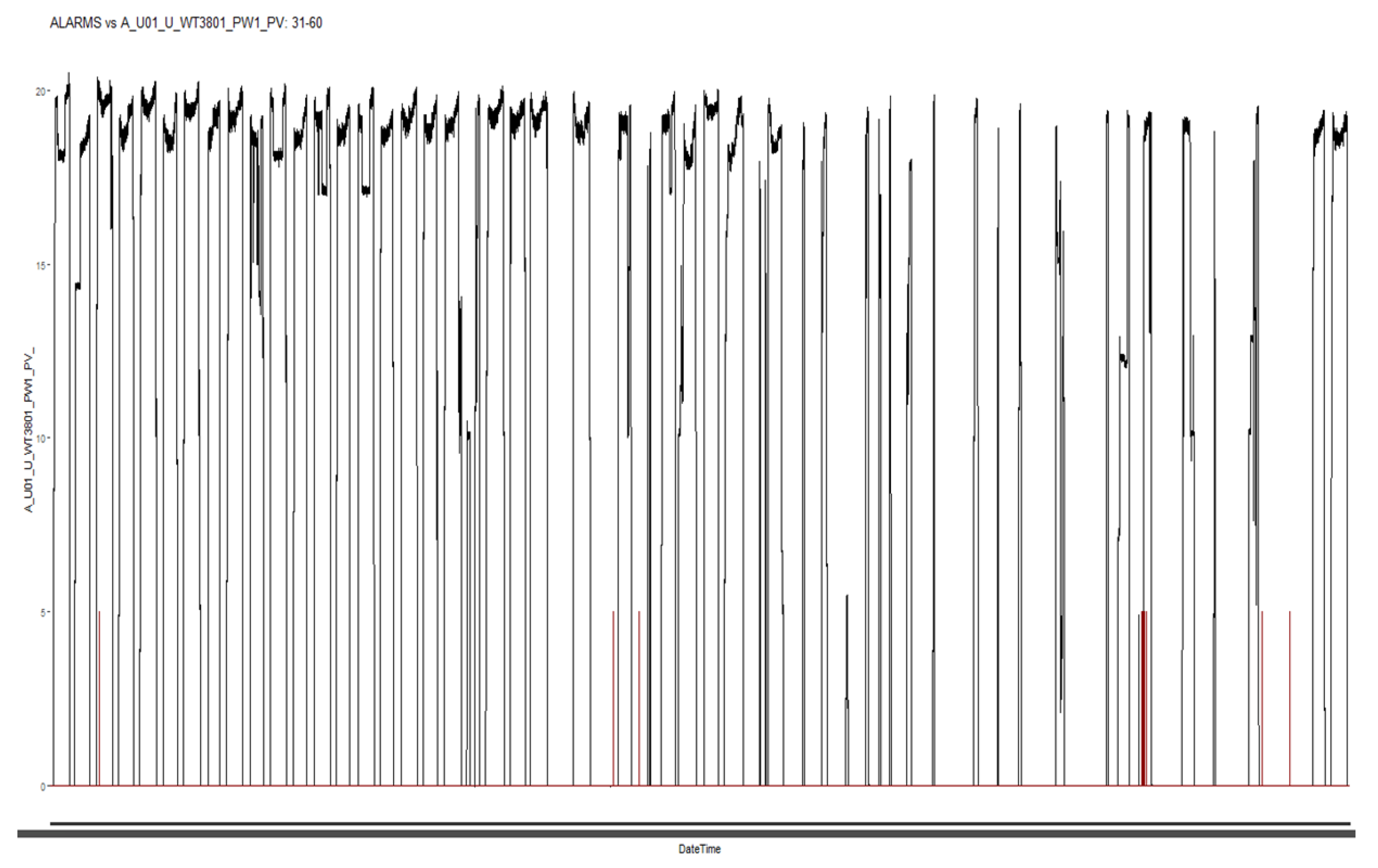
Figure 2.
An overview of the method.
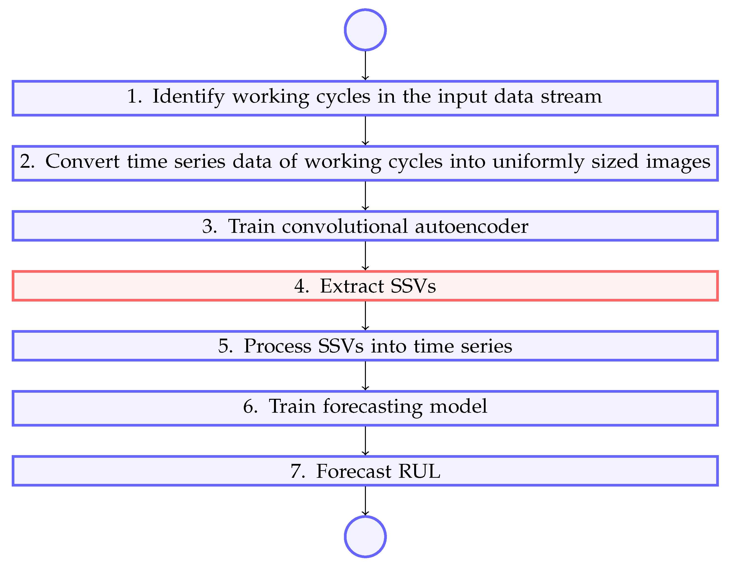
Figure 3.
An example of working cycle from historical data.
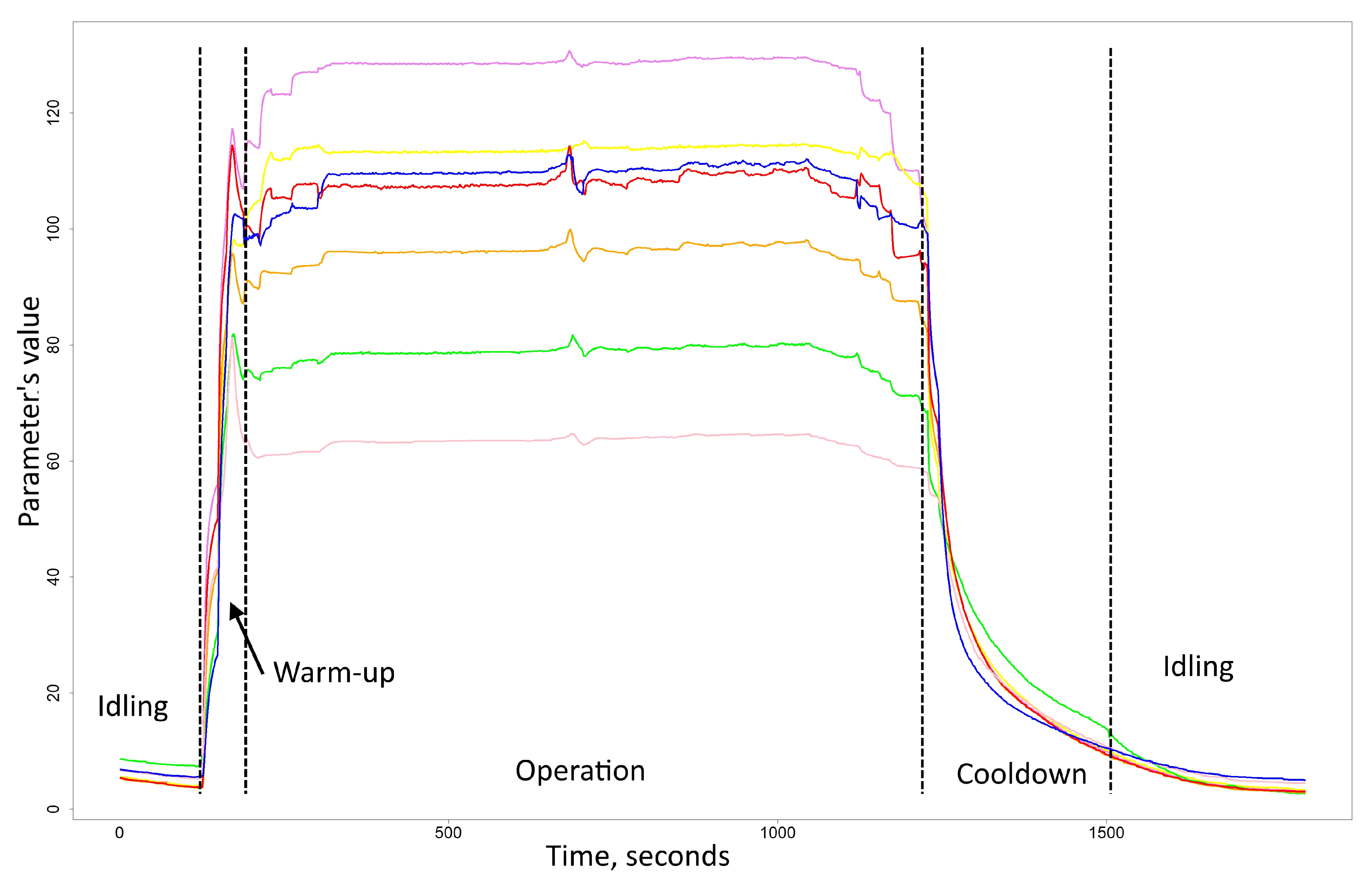
Figure 4.
Charts of the RUL forecast using different image sizes. X axis - number of working cycles, Y axis - RUL measured in number of working cycles
Figure 4.
Charts of the RUL forecast using different image sizes. X axis - number of working cycles, Y axis - RUL measured in number of working cycles
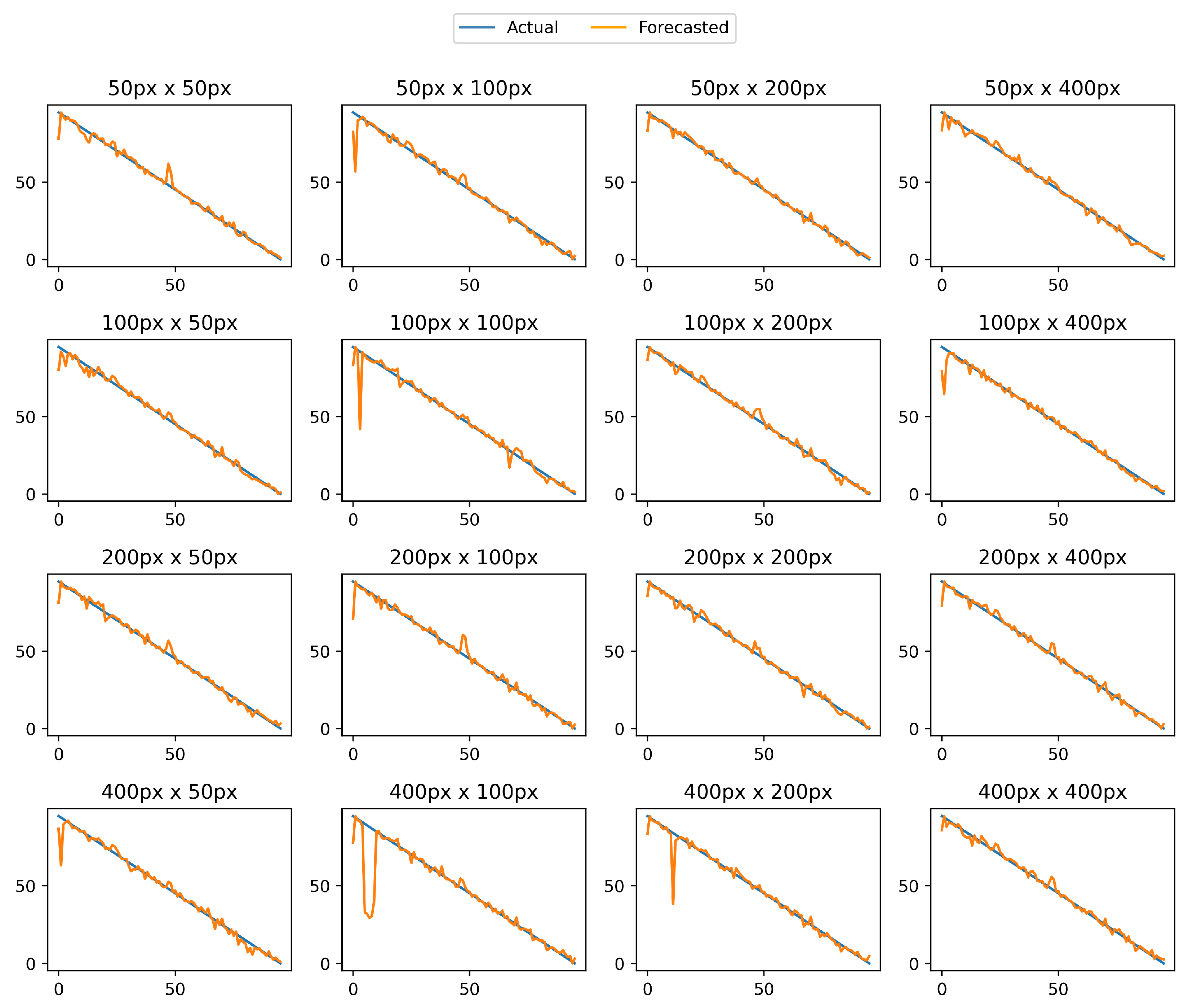
Figure 5.
A chart of the forecast RUL using 50x200 image size.
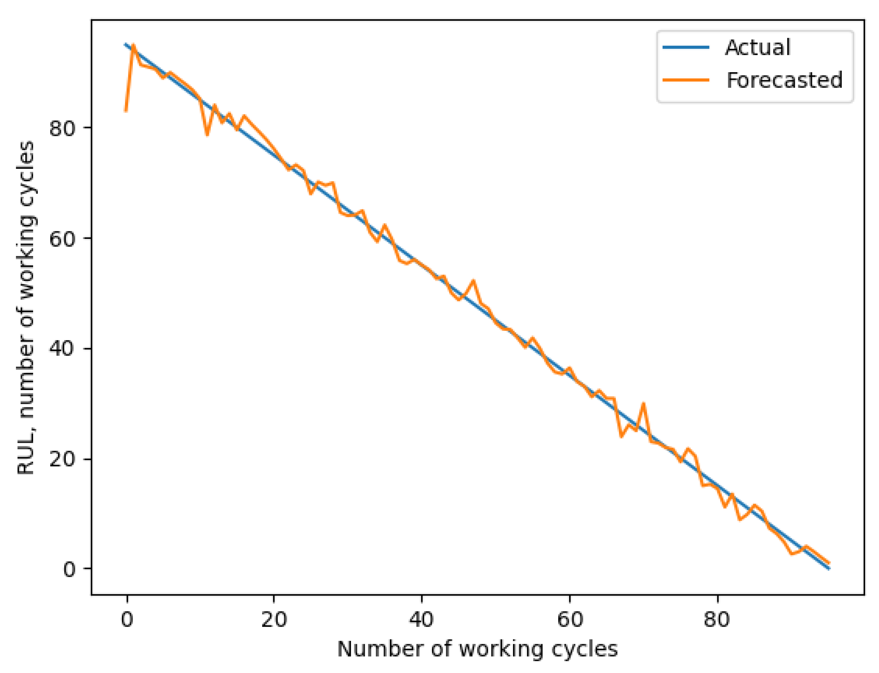
Figure 6.
A chart of the forecast RUL using vector length = 10.
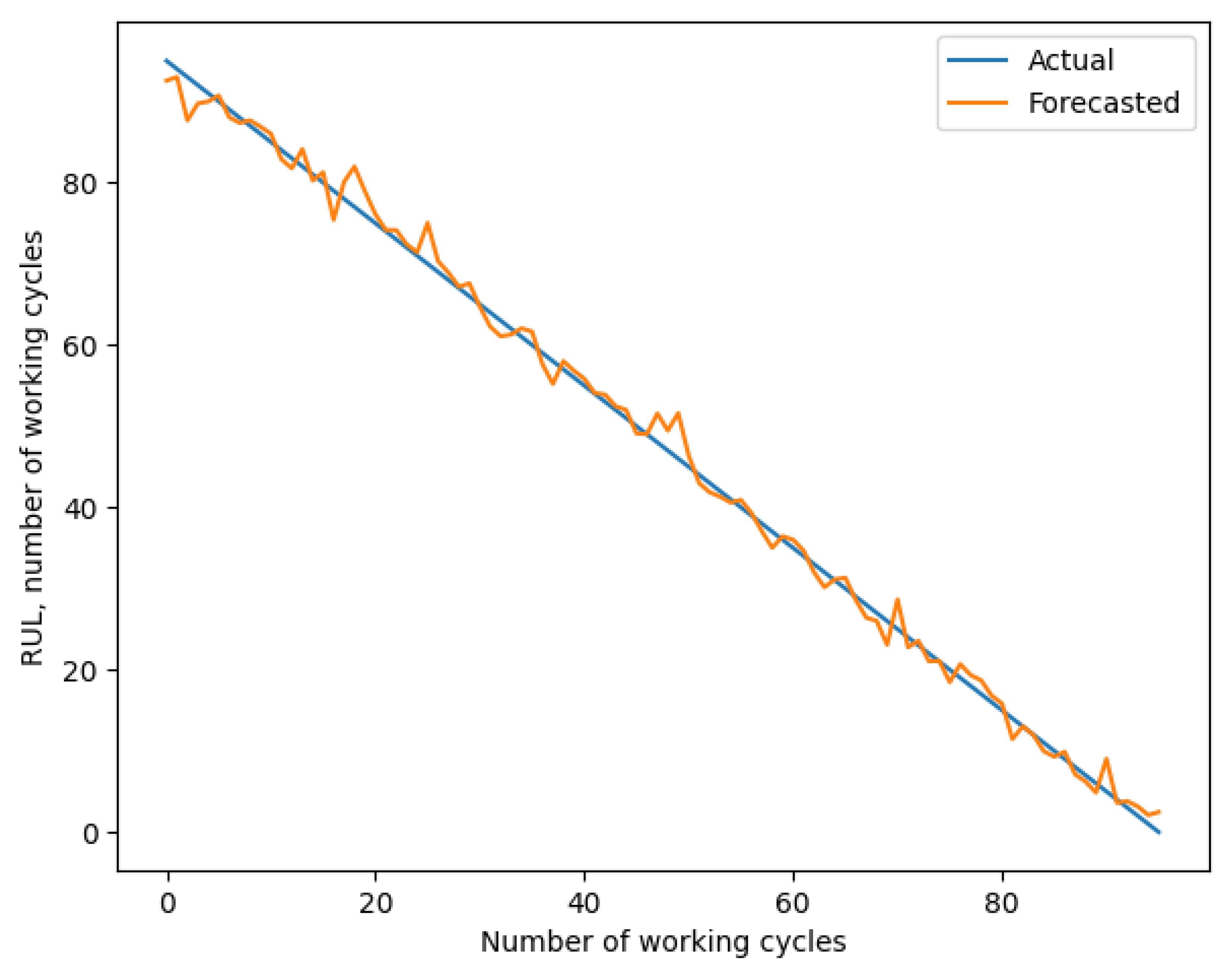

Table 1.
The architecture of the convolutional autoencoder.
| Layer | Parameters | Output shape |
|---|---|---|
| Convolution | Input shape: (200, 50, 3), kernel: 3x3, activation: ReLU, padding: same | (200, 50, 32) |
| Max pooling | window size: 2x1** | (100, 50, 32) |
| Convolution | kernel: 3x3, activation: ReLU, padding: same | (100, 50, 64) |
| Max pooling | window size: 4x5** | (25, 10, 64) |
| Convolution | kernel: 3x3, activation: ReLU, padding: same | (25, 10, 128) |
| Max pooling | window size: 5x5** | (5, 2, 128) |
| Convolution* | kernel: 3x3, activation: ReLU, padding: same | (5, 2, 32) |
| Dropout | rate: 0.5 | (5, 2, 32) |
| Convolution | kernel: 3x3, activation: ReLU, padding: same | (5, 2, 32) |
| Upsampling | size: 5x5** | (25, 10, 32) |
| Convolution | kernel: 3x3, activation: ReLU, padding: same | (25, 10, 128) |
| Upsampling | size: 4x5** | (100, 50, 128) |
| Convolution | kernel: 3x3, activation: ReLU, padding: same | (100, 50, 64) |
| Upsampling | size: 2x1** | (200, 50, 64) |
| Convolution | kernel: 3x3, activation: sigmoid, padding: same | (200, 50, 3) |
* output of this layer is used to create semantic state vector. ** variation of these sizes is used to adapt the model to different image sizes.
Table 2.
RMSE.
| Width\Height | 50px | 100px | 200px | 400px |
|---|---|---|---|---|
| 50px | 3.021 | 4.504 | 2.036 | 2.353 |
| 100px | 2.763 | 5.703 | 2.395 | 3.819 |
| 200px | 2.562 | 3.535 | 2.362 | 2.580 |
| 400px | 3.945 | 7.109 | 5.149 | 2.434 |
Table 3.
MAE.
| Width\Height | 50px | 100px | 200px | 400px |
|---|---|---|---|---|
| 50px | 1.742 | 2.084 | 1.405 | 1.631 |
| 100px | 1.860 | 2.212 | 1.725 | 1.828 |
| 200px | 1.717 | 1.890 | 1.676 | 1.624 |
| 400px | 2.037 | 2.629 | 2.005 | 1.806 |
Table 4.
Error measurements for different methods of conversion.
| Method | RMSE | MAE |
|---|---|---|
| Bilinear | 2.036 | 1.405 |
| Bicubic | 2.576 | 1.604 |
| Box | 2.237 | 1.516 |
| Hamming | 2.824 | 1.820 |
| Lanczos | 2.334 | 1.465 |
| Nearest | 2.312 | 1.750 |
Table 5.
Error measurements for different vector sizes.
| Vector size | RMSE | MAE |
|---|---|---|
| 5 | 5.845 | 2.056 |
| 10 | 1.799 | 1.374 |
| 25 | 2.036 | 1.405 |
| 50 | 5.467 | 2.418 |
| 100 | 5.955 | 2.351 |
Table 6.
Error measurements for different vector sizes.
| Method | RMSE | MAE |
|---|---|---|
| Semantic state vector extraction | 1.799 | 1.374 |
| MIN-AVG-MAX | 14.02 | 10.71 |
Disclaimer/Publisher’s Note: The statements, opinions and data contained in all publications are solely those of the individual author(s) and contributor(s) and not of MDPI and/or the editor(s). MDPI and/or the editor(s) disclaim responsibility for any injury to people or property resulting from any ideas, methods, instructions or products referred to in the content. |
© 2025 by the authors. Licensee MDPI, Basel, Switzerland. This article is an open access article distributed under the terms and conditions of the Creative Commons Attribution (CC BY) license (http://creativecommons.org/licenses/by/4.0/).
Copyright: This open access article is published under a Creative Commons CC BY 4.0 license, which permit the free download, distribution, and reuse, provided that the author and preprint are cited in any reuse.


