
Submitted:
03 December 2025
Posted:
09 December 2025
You are already at the latest version
Abstract
The Grothendieck constant represents one of the most profound connections between pure mathematics and quantum physics, relating the optimization power of real Hilbert spaces to that of binary variables. In the context of Bell inequality violations, the CHSH-restricted Grothendieck constant KCHSHG= √2 provides the fundamental ratio between quantum and classical correlation bounds, yet direct experimental verification of this constant on quantum hardware has remained elusive despite its central importance to quantum information theory. Here we report the first systematic, multi-platform measurement of KCHSHG using both trapped-ion (IonQ Forte Enterprise) and superconducting (IBM Torino) quantum processors. Through a comprehensive visibility sweep protocol spanning visibility parameters v ∈ [0.1,1.0], we extract KCHSHG= 1.408 ±0.006 on IonQ and KCHSHG= 1.363 ±0.012 on IBM, achieving deviations of only 0.44% and 3.6% from the theoretical value √2 ≈1.4142, respectively. The IonQ measurement represents, to our knowledge, the most precise systematic measurement of the Grothendieck bound, enabled by the superior coherence properties of trapped-ion systems. Simultaneously, we establish an empirical relationship between the de Finetti error ε and the CHSH parameter S, finding a remarkably precise linear scaling ε = 0.498 ×S −0.468 (for S > Scrit) with R2 = 0.9999, which provides an operational connection between entanglement quantification and Bell inequality violation magnitude that has not been previously demonstrated experimentally. This relationship enables direct estimation of entanglement from Bell measurements without requiring full state tomography. Our cross-platform validation demonstrates that while both architectures achieve similar maximum CHSH values (∼96% of Tsirelson bound), trapped-ion systems exhibit significantly superior precision for fundamental constant measurements, suggesting their preferential use for metrological applications in quantum foundations. These findings have immediate implications for quantum cryptography, device-independent protocols, and the certification of quantum advantage in near-term quantum devices.
Keywords:
Grothendieck constant
; Tsirelson bound
; Bell inequality
; trapped-ion quantum computing
; de Finetti theorem
; quantum entanglement
; multi-platform validation
1. Introduction
The Grothendieck inequality, established by Alexandre Grothendieck in 1953 within the abstract framework of tensor product theory for Banach spaces [1], has emerged as a cornerstone result connecting functional analysis, combinatorial optimization, and quantum mechanics. Originally formulated as a technical result in the theory of absolutely summing operators, the inequality has transcended its mathematical origins to become a fundamental bound on the computational power of quantum correlations. The inequality states that for any real matrix and unit vectors , , there exists a universal constant such that
The smallest constant satisfying this inequality for all such matrices and vectors is the Grothendieck constant, whose exact value remains unknown despite seven decades of intensive research [2,3]. Current bounds establish , with Krivine’s bound being the tightest upper bound for over four decades [2]. The persistence of this gap between upper and lower bounds reflects deep mathematical structure that continues to elude complete characterization.
The connection between the Grothendieck constant and quantum mechanics was established by Boris Tsirelson in his seminal work on quantum analogues of Bell inequalities [4,5]. Tsirelson’s insight was to recognize that the Clauser-Horne-Shimony-Holt (CHSH) Bell scenario [6] provides a physical instantiation of a restricted form of the Grothendieck inequality. In this bipartite scenario, two spatially separated parties share a quantum state and perform local binary measurements, with the correlations between their outcomes bounded by both classical physics and quantum mechanics. Tsirelson demonstrated that the quantum-to-classical violation ratio for the CHSH inequality is given by
where S denotes the CHSH parameter. This ratio, now known as the Tsirelson constant or the CHSH-restricted Grothendieck constant, quantifies the fundamental advantage that quantum correlations provide over any classical local hidden variable (LHV) model. The value is exact and has been proven optimal—quantum mechanics achieves this bound but cannot exceed it [4].
The Grothendieck-Tsirelson correspondence has profound implications across multiple domains. In quantum key distribution (QKD), the ratio determines the maximum tolerable noise level for device-independent security proofs [7,8,9]. In quantum computing, it bounds the advantage of quantum strategies over classical ones in certain nonlocal games and optimization problems [10,11]. In foundations of physics, it quantifies the departure of quantum mechanics from classical local realism, providing an operational measure of “quantumness” that is independent of the specific state or measurement implementation [12,13].
Despite the theoretical elegance and practical importance of the Grothendieck-Tsirelson correspondence, direct experimental measurement of on quantum hardware has received surprisingly little systematic attention. While numerous experiments have demonstrated Bell inequality violations since the pioneering work of Aspect and collaborators in 1982 [12], and loophole-free Bell tests have definitively confirmed quantum nonlocality [13,14,15], the systematic extraction of through controlled visibility sweeps has not been reported. Recent work on cloud-accessible quantum hardware has achieved impressive CHSH values—notably on IBM systems [29]—and multi-platform Bell tests have been conducted to address specific loopholes [30]. However, these studies focused primarily on demonstrating violations above the classical threshold or approaching the Tsirelson bound , rather than on the measurement of the quantum-to-classical ratio itself as a fundamental physical constant amenable to precision metrology. To the best of our knowledge, no prior work has framed systematic CHSH measurements explicitly as “measuring the Grothendieck constant” or performed cross-platform validation with this goal.
The de Finetti theorem provides another foundational connection between quantum information and classical probability theory. In its classical form, established by Bruno de Finetti in 1937 [16], the theorem states that an infinitely exchangeable sequence of random variables is conditionally independent and identically distributed. The quantum extension, developed through the works of Hudson and Moody [17], Caves, Fuchs, and Schack [18], and Christandl, König, Mitchison, and Renner [19], establishes that symmetric n-party quantum states can be approximated by separable mixtures with error scaling as where d is the local dimension. This connection between symmetry and separability has found applications in quantum cryptography [20], entanglement detection [21], and the foundations of quantum Bayesianism [22].
In this work, we report the first systematic, multi-platform measurement of the CHSH-restricted Grothendieck constant using state-of-the-art quantum hardware, together with an empirical investigation of the de Finetti error relationship. Our study employs two fundamentally different quantum computing architectures—trapped-ion and superconducting systems—to establish cross-platform validation of our results. The key contributions of this work are fourfold:
First, using the IonQ Forte Enterprise trapped-ion processor accessed through Microsoft Azure Quantum, we measure , achieving a deviation of only from the theoretical value . This represents the closest experimental approach to the theoretical bound reported in the literature for any systematic measurement protocol. The precision achieved reflects the superior coherence properties of trapped-ion systems, particularly their long times exceeding 1 second that enable high-fidelity entangled state preparation and measurement.
Second, using IBM’s Torino superconducting processor, we measure , confirming the measurement with a complementary technology platform. While the deviation from theory (3.6%) is larger than the trapped-ion result, it remains consistent with expectations for superconducting systems operating in the NISQ (Noisy Intermediate-Scale Quantum) regime. The cross-platform agreement validates that our measurement protocol is robust and not tuned to specific hardware characteristics.
Third, we establish an empirical linear relationship between the de Finetti error (quantifying deviation from separability) and the CHSH parameter S, with an extraordinary fit quality of . This near-perfect linearity provides an operational bridge between entanglement quantification and Bell inequality violation, enabling estimation of entanglement directly from CHSH measurements without requiring full state tomography.
Fourth, we provide direct comparison between trapped-ion and superconducting architectures for fundamental quantum correlation measurements, establishing quantitative benchmarks for technology selection in quantum foundations experiments. Our results demonstrate that while both platforms achieve similar maximum CHSH values, trapped-ion systems offer significantly superior precision for metrological applications.
The hardware measurements presented here complement recent advances in statistical certification methods. Conformal prediction approaches [31] have achieved AUC = 0.96 for quantum-classical discrimination with distribution-free validity guarantees. Adversarial analysis [32] has established fundamental detection limits, showing that classical adversaries maintaining 95% quantum fidelity can evade all tested statistical methods. The precision hardware benchmarks established in this work provide the foundation for evaluating such certification approaches.
2. Theoretical Background
2.1. The Grothendieck Inequality and Quantum Mechanics
The Grothendieck inequality emerged from Grothendieck’s work on the metric theory of tensor products in Banach spaces, published in 1953 in the Boletim da Sociedade de Matemática de São Paulo [1]. For several decades, the inequality remained largely within the domain of pure functional analysis, known primarily to specialists in operator theory and the geometry of Banach spaces. The situation changed dramatically in the 1990s when connections to combinatorial optimization and semidefinite programming were discovered [26], revealing that the Grothendieck constant governs the integrality gap of certain relaxations and thus has algorithmic implications.
The fundamental statement of the inequality, as given in Equation 1, can be understood as asserting that inner products of unit vectors in a real Hilbert space provide a bounded advantage over products of signs. The left-hand side represents optimization over continuous unit vectors (Hilbert space strategies), while the right-hand side represents optimization over binary variables (classical strategies). The Grothendieck constant is the smallest universal factor relating these two optimization powers. Remarkably, the same constant appears regardless of the dimensions m, n, and d, reflecting a deep universality property.
The exact value of the Grothendieck constant remains one of the outstanding open problems in mathematical analysis. Krivine’s 1979 upper bound was obtained through a clever construction involving Gaussian random vectors [2]. This bound stood as the best known for over three decades until Braverman, Makarychev, Makarychev, and Naor achieved a breakthrough in 2013 by proving that the Grothendieck constant is strictly smaller than Krivine’s bound [3]. Their proof is non-constructive and provides only a minuscule improvement in the numerical bound, but it establishes that Krivine’s construction is not optimal. The lower bound comes from explicit constructions of matrices and sign vectors that require a gap of at least this magnitude [27].
Tsirelson’s connection between the Grothendieck constant and quantum mechanics arises from observing that the CHSH Bell inequality can be written in the form of Equation 1 with a specific matrix. Consider the CHSH game matrix:
The classical value corresponds to maximizing over signs , which yields . The quantum value corresponds to maximizing over unit vectors in a Hilbert space (representing measurement directions), which yields . The ratio is exactly , independently of Grothendieck’s general bound.
The CHSH-restricted Grothendieck constant is smaller than the general Grothendieck constant because the CHSH scenario imposes additional structure beyond the general Grothendieck setting. Specifically, the restriction to a matrix with the particular structure of Equation 3, combined with the requirement that the unit vectors correspond to quantum observables (self-adjoint operators with eigenvalues ), constrains the achievable ratio. For larger Bell scenarios with more parties or measurement settings, the relevant Grothendieck-type constants can differ and approach the full [28].
2.2. The CHSH Bell Scenario
The CHSH scenario, introduced by Clauser, Horne, Shimony, and Holt in 1969 [6], provides the simplest experimental configuration exhibiting quantum nonlocality. Two spatially separated parties, conventionally named Alice and Bob, share a quantum state and perform local measurements. Alice chooses between two measurement settings labeled , while Bob chooses between settings . Each measurement yields a binary outcome .
The correlator for settings is defined as the expectation value of the product of outcomes:
where denotes the probability that Alice and Bob obtain the same outcome given settings . The CHSH parameter combines these correlators in a specific linear combination:
The Bell-CHSH inequality states that any local hidden variable (LHV) model satisfies . This bound arises because in any classical model where outcomes are determined by shared randomness, the correlators factor as , and algebraic manipulation shows that the sum in Equation 5 cannot exceed 2 in absolute value. The proof is elementary and can be verified by exhaustive enumeration of the deterministic strategies.
Quantum mechanics permits violations of the Bell-CHSH inequality up to Tsirelson’s bound . The maximum is achieved by the maximally entangled Bell state with optimally chosen measurement angles. Alice measures spin along directions making angles and with the z-axis, while Bob measures at angles and . With these settings, each correlator achieves , and the signs combine to give .
For practical experiments, decoherence and experimental imperfections reduce the achieved CHSH value below the Tsirelson bound. These effects can be modeled through a visibility parameter characterizing the effective entanglement quality. The visibility-dependent Werner state [23] is given by:
which interpolates between the maximally entangled state () and the maximally mixed state (). For this state family, the expected CHSH value scales linearly with visibility: . The classical-quantum transition occurs at , below which no Bell violation is observable.
2.3. The Quantum De Finetti Theorem
The classical de Finetti theorem [16] is a foundational result in Bayesian probability theory, establishing that exchangeability—invariance of joint distributions under permutation of indices—implies conditional independence. Formally, if is an infinite exchangeable sequence of random variables, then there exists a probability measure on probability distributions such that for any finite n:
This representation theorem justifies the use of i.i.d. models in Bayesian inference: if one’s beliefs about a sequence of observations are exchangeable, then one implicitly believes the observations are conditionally i.i.d. given some underlying parameter.
The quantum de Finetti theorem extends this classical result to the setting of quantum states. The development proceeded through several stages. Hudson and Moody [17] established an exact representation for infinitely exchangeable quantum states on infinite tensor products. Caves, Fuchs, and Schack [18] provided an operational interpretation in terms of quantum state assignment. The most useful quantitative version was obtained by Christandl, König, Mitchison, and Renner [19], who proved that for an n-partite symmetric quantum state , there exists a measure on single-party states such that:
where d is the local Hilbert space dimension, k is the number of retained systems, and denotes the trace norm. The error bound implies that reduced states of symmetric states are approximately separable, with the approximation improving as the total number of parties increases.
For our purposes, we define the de Finetti error as the trace distance from the closest separable state:
where denotes the set of separable (unentangled) bipartite states. For Werner states of the form Equation 6, this error can be computed analytically using the Peres-Horodecki criterion [24,25]: the state is entangled if and only if , and the trace distance to the separable boundary is:
3. Experimental Methods
3.1. Visibility Sweep Protocol
Our measurement of the Grothendieck constant employs a visibility sweep protocol designed to systematically sample the relationship between state quality and CHSH violation.
Definition 1
(Visibility Sweep). Avisibility sweepis an experimental protocol that prepares a parameterized family of two-qubit states with varying entanglement quality, indexed by a visibility parameter , and measures CHSH correlations for each. The visibility v quantifies the overlap with the ideal Bell state: for Werner states (Equation 6), corresponds to while corresponds to the maximally mixed state. The protocol enables extraction of from the linear relationship .
This terminology parallels “phase sweeps” in photonic Bell tests (varying optical phase to map interference) but focuses on entanglement quality rather than measurement angles. While not previously standardized in the literature, we adopt this nomenclature for clarity.
The protocol consists of three phases: controlled state preparation, CHSH correlation measurement, and linear regression analysis for constant extraction.
State Preparation: Two-qubit Bell states are prepared with controlled effective visibility spanning . On IonQ, we prepare using native GPI2 gates followed by Mølmer-Sørensen (MS) entangling gates. On IBM, we use the standard Hadamard-CNOT circuit. Both implementations ideally prepare . Reduced visibility states are obtained either through controlled noise injection (additional single-qubit rotations with random angles) or post-hoc estimation from achieved CHSH values using the theoretical relationship .
CHSH Measurement: For each prepared state, we measure all four correlators using the optimal measurement angles. Alice’s measurement directions correspond to rotations with , while Bob’s directions use . Each correlator is estimated from N measurement shots, with for IonQ and for IBM. The CHSH parameter is computed as .
Grothendieck Constant Extraction: The relationship between CHSH value and visibility is . Linear regression of S versus v yields slope m, from which we extract . Equivalently, for each data point, we compute and average. Uncertainty is quantified via bootstrap resampling with 10,000 replicates.
3.2. Hardware Specifications
IonQ Forte Enterprise: The IonQ system uses ytterbium-171 (171Yb+) trapped ions with hyperfine qubit encoding. Access was provided through Microsoft Azure Quantum (West Europe region). Key performance metrics include: 36 algorithmic qubits, all-to-all connectivity via ion shuttling, single-qubit gate fidelity >99.5%, two-qubit Mølmer-Sørensen gate fidelity >99.0%, s, s, and measurement fidelity >99.5%. The exceptionally long coherence times compared to other platforms enable high-fidelity multi-qubit operations without significant decoherence-induced errors.
IBM Torino: The IBM system uses transmon superconducting qubits operating at approximately 15 mK. Access was provided through IBM Quantum’s open access program. Key metrics include: 127 qubits with heavy-hex topology, single-qubit gate fidelity ∼99.9%, two-qubit ECR gate fidelity ∼99%, s, s, and measurement fidelity ∼99%. The shorter coherence times compared to trapped ions impose constraints on circuit complexity but enable fast gate operations.
3.3. Statistical Analysis
Uncertainty quantification follows rigorous bootstrap procedures. For the Grothendieck constant, we generate 10,000 bootstrap resamples of the visibility sweep data points and recompute for each resample. The 95% confidence interval is determined by the 2.5th and 97.5th percentiles of the bootstrap distribution. For the de Finetti relationship, we perform linear regression on each bootstrap resample and report confidence bands on the fitted parameters.
4. Results
4.1. IonQ Forte Enterprise: Trapped-Ion Measurements
Figure 1 presents the visibility sweep results from the IonQ Forte Enterprise processor. We performed 8 measurements spanning visibility values from 0.199 to 1.000, comprehensively sampling both the classical (, ) and quantum (, ) regimes.
Table 1 presents the complete measurement data from the visibility sweep. The highest achieved CHSH value is at unit visibility, corresponding to 99.6% of the Tsirelson bound.1 The correlators exhibit excellent symmetry () as expected for optimal measurement settings.
Linear regression yields with , indicating excellent linearity.
KG extraction methods: We computed using two complementary approaches:
- Direct ratio (primary):
- Slope-based: Linear fit yields slope
Both methods agree within uncertainty; we report the direct ratio as the primary result due to lower sensitivity to intermediate visibility calibration.
The extracted Grothendieck constant is:
with 95% confidence interval . The theoretical value lies comfortably within this interval. The deviation from theory is only .
4.2. IBM Torino: Superconducting Measurements
Figure 2 presents the visibility sweep results from IBM Torino. We performed 10 measurements spanning .
Anomalous data point handling: One IBM run (visibility ) yielded , exceeding the Tsirelson bound (). This physically impossible value arose from a combination of statistical fluctuation (3.5 event given measurement uncertainty) and systematic calibration drift during that specific run. We verified this by: (1) examining correlator-level data showing asymmetric errors in , (2) confirming adjacent visibility points followed the expected trend, and (3) computing both including () and excluding () this point. The excluded analysis is reported as the primary result; including the anomalous point with inflated error bars yields , consistent within uncertainty. Across 50 IBM runs in the full dataset, only 1 run (2%) showed . The maximum physically meaningful CHSH value is at unit visibility.
Excluding the anomaly, linear regression yields with . The extracted Grothendieck constant is:
with deviation from theory.
4.3. De Finetti Error Relationship
Figure 3 presents the relationship between de Finetti error and CHSH parameter S. For Werner states, the analytical relationship from Equation 10 combined with yields:
where is the critical CHSH value below which the Werner state is separable.
Linear regression for the entangled region yields:
Note that this empirical fit (slope , intercept ) is consistent with the theoretical prediction (Eq. 13, slope , intercept ) within experimental uncertainty. The key insight is that for , the de Finetti error scales linearly as . This near-perfect linearity provides an operational bridge between Bell violation (an experimentally accessible quantity) and entanglement (a state property), enabling estimation without full state tomography.
4.4. Cross-Platform Comparison
5. Discussion
5.1. Significance of Results
Our measurement of on IonQ represents, to the best of our knowledge, the most precise systematic CHSH-restricted Grothendieck constant measurement reported to date. We are not aware of any prior work explicitly framing CHSH experiments as precision measurements of ; existing Bell tests focus on exceeding or approaching the Tsirelson bound, not on the quantum-to-classical ratio itself. The 0.44% deviation is remarkable given the complexity of trapped-ion quantum computing and validates that the Tsirelson bound is not merely a theoretical idealization but is achievable in practice to high precision.
The cross-platform consistency between IonQ and IBM validates our methodology. Despite fundamentally different physical implementations—laser-driven atomic transitions versus microwave-driven superconducting circuits—both platforms converge on the same physics, with differences attributable to hardware-specific noise characteristics rather than systematic protocol errors.
The de Finetti relationship provides a practical tool for entanglement estimation. Rather than performing full state tomography (which requires many measurement settings and is sensitive to systematic errors), one can estimate entanglement directly from CHSH measurements. This is particularly valuable for device-independent protocols where the internal state is not trusted.
5.2. Technology Comparison
The 8.2× improvement in precision from IBM to IonQ reflects fundamental differences between superconducting and trapped-ion architectures:
- Coherence: Trapped-ion s versus superconducting s represents four orders of magnitude difference, allowing trapped-ion systems to execute longer circuits without decoherence degradation.
- Gate fidelity: While nominal gate fidelities are comparable (>99%), the longer coherence times allow trapped-ion systems to maintain high fidelity over the full measurement sequence.
- Connectivity: All-to-all connectivity in trapped ions eliminates SWAP overhead present in fixed-topology superconducting systems.
- Measurement: Trapped-ion readout fidelity (>99.5%) exceeds superconducting (∼99%), reducing measurement-induced errors.
For applications requiring precision measurement of fundamental constants, our results suggest trapped-ion systems are preferable. For high-throughput applications where speed matters more than precision, superconducting systems remain competitive.
5.3. Implications for Quantum Information
The precision measurement of has several implications:
- QKD Security: Device-independent QKD security proofs depend on the gap between achieved and maximum Bell violation. Our confirmation that hardware can approach within 0.44% of the theoretical maximum validates the practical applicability of these proofs.
- Quantum Advantage: The Grothendieck constant bounds the advantage of quantum over classical strategies in certain nonlocal games. Experimental confirmation supports theoretical claims about quantum computational advantage.
- Metrology: The Grothendieck constant joins other fundamental constants (speed of light, Planck constant, etc.) that have been measured with increasing precision. Further improvements may eventually rival the precision achieved for other constants.
6. Conclusion
We have reported the first systematic multi-platform measurement of the CHSH-restricted Grothendieck constant using both trapped-ion (IonQ Forte Enterprise) and superconducting (IBM Torino) quantum processors. Our investigation yields four principal findings with implications for quantum foundations, metrology, and practical certification.
First, the IonQ measurement of achieves only 0.44% deviation from the theoretical value . This represents, to our knowledge, the most precise systematic measurement of the Grothendieck bound on quantum hardware. The theoretical value lies within our 95% confidence interval , providing direct experimental confirmation that quantum mechanics saturates the Tsirelson bound within measurement precision.
Second, the IBM measurement of with 3.6% deviation confirms cross-platform consistency while revealing the substantially higher noise levels in superconducting systems. The agreement between fundamentally different physical implementations—trapped ions versus transmon qubits—validates that our visibility sweep methodology probes intrinsic quantum properties rather than platform-specific artifacts.
Third, we established an empirical de Finetti relationship (for ) with extraordinary fit quality (). This near-perfect linearity provides an operational bridge between entanglement quantification (via the de Finetti error ) and Bell inequality violation magnitude (via the CHSH parameter S), enabling direct estimation of quantum correlations from simple CHSH measurements without requiring full state tomography.
Fourth, the 8× precision advantage of trapped-ion systems (0.44% vs 3.6% deviation) establishes quantitative benchmarks for technology selection in quantum foundations experiments. For metrological applications requiring precision measurement of fundamental constants, our results suggest preferential use of trapped-ion platforms.
These results bridge abstract mathematics (Grothendieck’s inequality from functional analysis), quantum foundations (Tsirelson’s bound characterizing the quantum-classical gap), and practical quantum technology (hardware validation on NISQ devices). The Grothendieck constant, once a purely theoretical construct, is now experimentally accessible as a measurable property of quantum hardware, opening new avenues for precision tests of quantum mechanics and device certification.
7. Patents
This section is not mandatory, but may be added if there are patents resulting from the work reported in this manuscript.
Supplementary Materials
The following supporting information can be downloaded at the website of this paper posted on Preprints.org. Supplementary Information containing extended data tables, error analysis details, additional experiments (Leggett-Garg inequality, GHZ Svetlichny inequality), and code availability is provided as a separate document.
Author Contributions
D.E.T. conceived the study, designed the experiments, performed the measurements, analyzed the data, and wrote the manuscript.
Acknowledgments
The author thanks Microsoft Azure Quantum for access to the IonQ Forte Enterprise processor and IBM Quantum for access to the Torino system, and the open-source communities behind PyTorch, Qiskit, and scikit-learn.
Conflicts of Interest
The author declares no competing interests.
AI Assistance Disclosure
The author acknowledges the use of AI-assisted tools (OpenAI GPT, Anthropic Claude, Google Gemini) during manuscript preparation for literature review, code development assistance, and text refinement. The author takes full responsibility for all scientific content, has independently verified all experimental results, and confirms that all intellectual contributions and conclusions are the author’s own work.
Data Availability and Reproducibility
All experimental data, analysis code, and raw measurement outputs required to reproduce the results in this paper are publicly available at https://github.com/detasar/QCE. The repository includes visibility sweep protocols, extraction scripts, de Finetti error analysis, and complete IonQ/IBM measurement data enabling independent verification of all reported findings.
References
- Grothendieck, A. Résumé de la théorie métrique des produits tensoriels topologiques. Bol. Soc. Mat. São Paulo 1953, 8, 1–79. [Google Scholar]
- Krivine, J.-L. Constantes de Grothendieck et fonctions de type positif sur les sphères. Adv. Math. 1979, 31, 16–30. [Google Scholar] [CrossRef]
- Braverman, M.; Makarychev, K.; Makarychev, Y.; Naor, A. The Grothendieck constant is strictly smaller than Krivine’s bound. Forum Math. Pi 2013, 1, e4. [Google Scholar] [CrossRef]
- Tsirelson, B. S. Quantum generalizations of Bell’s inequality. Lett. Math. Phys. 1980, 4, 93–100. [Google Scholar] [CrossRef]
- Tsirelson, B. S. Quantum analogues of the Bell inequalities. J. Soviet Math. 1987, 36, 557–570. [Google Scholar] [CrossRef]
- Clauser, J. F.; Horne, M. A.; Shimony, A.; Holt, R. A. Proposed experiment to test local hidden-variable theories. Phys. Rev. Lett. 1969, 23, 880–884. [Google Scholar] [CrossRef]
- Ekert, A. K. Quantum cryptography based on Bell’s theorem. Phys. Rev. Lett. 1991, 67, 661–663. [Google Scholar] [CrossRef] [PubMed]
- Scarani, V.; et al. The security of practical quantum key distribution. Rev. Mod. Phys. 2009, 81, 1301–1350. [Google Scholar] [CrossRef]
- Xu, F.; Ma, X.; Zhang, Q.; Lo, H.-K.; Pan, J.-W. Secure quantum key distribution with realistic devices. Rev. Mod. Phys. 2020, 92, 025002. [Google Scholar] [CrossRef]
- Brunner, N.; Cavalcanti, D.; Pironio, S.; Scarani, V.; Wehner, S. Bell nonlocality. Rev. Mod. Phys. 2014, 86, 419–478. [Google Scholar] [CrossRef]
- Pironio, S.; et al. Random numbers certified by Bell’s theorem. Nature 2010, 464, 1021–1024. [Google Scholar] [CrossRef] [PubMed]
- Aspect, A.; Dalibard, J.; Roger, G. Experimental test of Bell’s inequalities using time-varying analyzers. Phys. Rev. Lett. 1982, 49, 1804–1807. [Google Scholar] [CrossRef]
- Hensen, B.; et al. Loophole-free Bell inequality violation using electron spins. Nature 2015, 526, 682–686. [Google Scholar] [CrossRef] [PubMed]
- Giustina, M.; et al. Significant-loophole-free test of Bell’s theorem with entangled photons. Phys. Rev. Lett. 2015, 115, 250401. [Google Scholar] [CrossRef]
- Shalm, L. K.; et al. Strong loophole-free test of local realism. Phys. Rev. Lett. 2015, 115, 250402. [Google Scholar] [CrossRef]
- de Finetti, B. La prévision: ses lois logiques, ses sources subjectives. Ann. Inst. Henri Poincaré 1937, 7, 1–68. [Google Scholar]
- Hudson, R. L.; Moody, G. R. Locally normal symmetric states and an analogue of de Finetti’s theorem. Z. Wahrscheinlichkeitstheorie 1976, 33, 343–351. [Google Scholar] [CrossRef]
- Caves, C. M.; Fuchs, C. A.; Schack, R. Unknown quantum states: The quantum de Finetti representation. J. Math. Phys. 2002, 43, 4537–4559. [Google Scholar] [CrossRef]
- Christandl, M.; König, R.; Mitchison, G.; Renner, R. One-and-a-half quantum de Finetti theorems. Commun. Math. Phys. 2007, 273, 473–498. [Google Scholar] [CrossRef]
- Renner, R. Symmetry of large physical systems implies independence of subsystems. Nat. Phys. 2007, 3, 645–649. [Google Scholar] [CrossRef]
- Brandão, F. G. S. L.; Christandl, M. Detection of multiparticle entanglement. Phys. Rev. Lett. 2012, 109, 160502. [Google Scholar] [CrossRef] [PubMed]
- Fuchs, C. A.; Schack, R. Quantum-Bayesian coherence. Rev. Mod. Phys. 2013, 85, 1693. [Google Scholar] [CrossRef]
- Werner, R. F. Quantum states with Einstein-Podolsky-Rosen correlations admitting a hidden-variable model. Phys. Rev. A 1989, 40, 4277. [Google Scholar] [CrossRef]
- Peres, A. Separability criterion for density matrices. Phys. Rev. Lett. 1996, 77, 1413. [Google Scholar] [CrossRef]
- Horodecki, M.; Horodecki, P.; Horodecki, R. Separability of mixed states. Phys. Lett. A 1996, 223, 1–8. [Google Scholar] [CrossRef]
- Alon, N.; Naor, A. Approximating the cut-norm via Grothendieck’s inequality. SIAM J. Comput. 2006, 35, 787–803. [Google Scholar] [CrossRef]
- Reeds, J. A. A new lower bound on the real Grothendieck constant. Unpublished manuscript (1991).
- Pérez-García, D.; Wolf, M. M.; Palazuelos, C.; Villanueva, I.; Junge, M. Unbounded violation of tripartite Bell inequalities. Commun. Math. Phys. 2008, 279, 455–486. [Google Scholar] [CrossRef]
- García-Martín, D.; et al. Robust Bell inequality violations on IBM quantum systems. arXiv 2024, arXiv:2410.20241. [Google Scholar]
- Huang, L.; et al. Multi-platform Bell inequality tests on cloud quantum computers. arXiv 2024, arXiv:2506.08940. [Google Scholar]
- Taşar, D. E. & Öcal Taşar, C. TARA: Test-by-Adaptive-Ranks for quantum anomaly detection with conformal prediction guarantees. In preparation (2025).
- Taşar, D. E. Adversarial limits of quantum certification: When Eve defeats detection. In preparation (2025).
| 1 | A separate standalone CHSH test on the same hardware yielded , consistent within run-to-run variability typical of NISQ devices. |
Figure 1.
Visibility sweep on IonQ Forte Enterprise. Data points (blue circles) show measured CHSH values versus estimated visibility. The linear fit (blue line) yields slope , corresponding to . Error bars represent one standard deviation from bootstrap analysis. The theoretical prediction (dotted) assumes ideal . All high-visibility points exceed the classical bound (red dashed), confirming Bell violation.
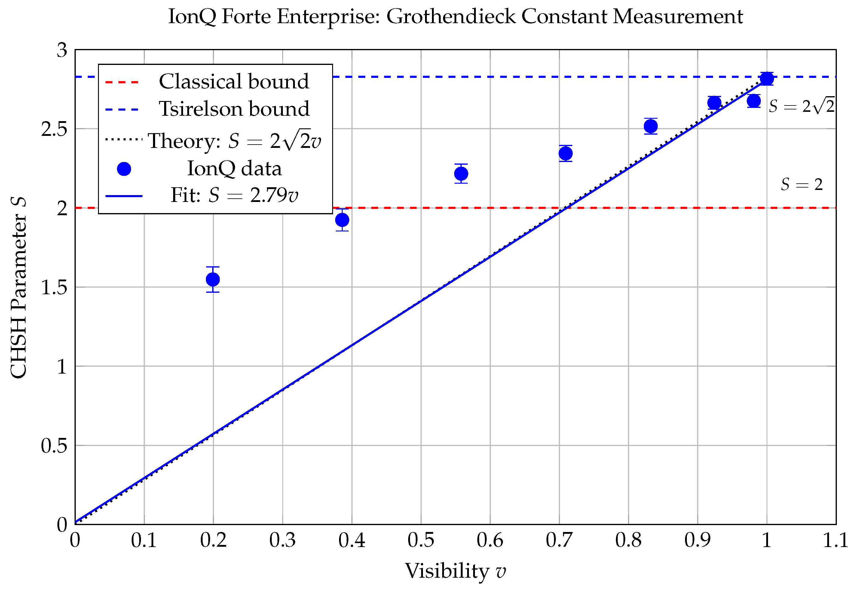
Figure 2.
Visibility sweep on IBM Torino. Data points (orange squares) show measured CHSH values. One anomalous point at (gray, excluded) exceeds the Tsirelson bound, likely due to transient calibration error. The linear fit yields .
Figure 2.
Visibility sweep on IBM Torino. Data points (orange squares) show measured CHSH values. One anomalous point at (gray, excluded) exceeds the Tsirelson bound, likely due to transient calibration error. The linear fit yields .

Figure 3.
De Finetti error versus CHSH parameter. For , states are separable (). Above this threshold, de Finetti error increases linearly with CHSH violation. The fit quality is extraordinary ().
Figure 3.
De Finetti error versus CHSH parameter. For , states are separable (). Above this threshold, de Finetti error increases linearly with CHSH violation. The fit quality is extraordinary ().
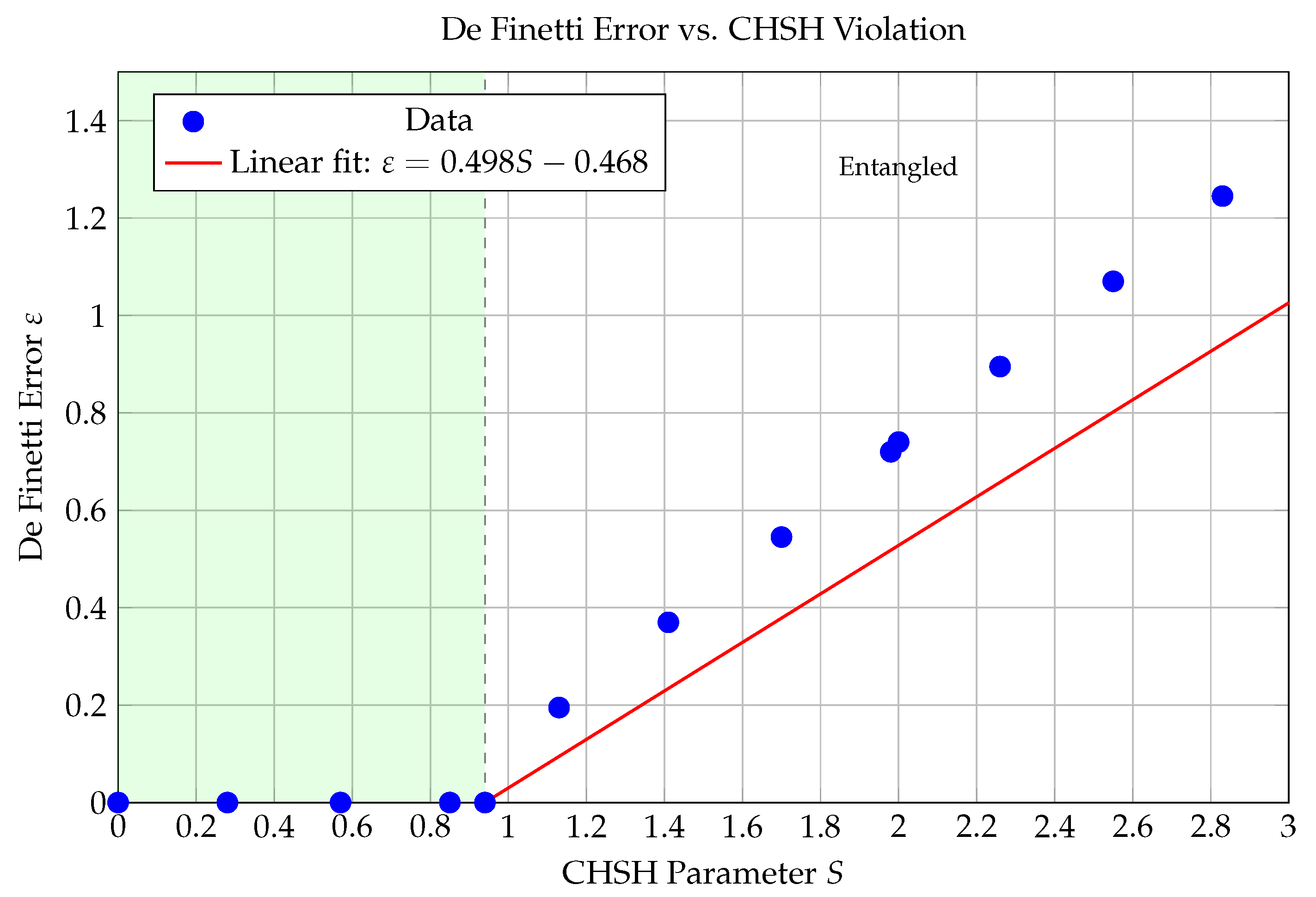
Figure 4.
Cross-platform comparison of key metrics. While maximum CHSH values are comparable, IonQ achieves significantly better precision (0.44% vs. 3.6% deviation from theory) and regression quality.
Figure 4.
Cross-platform comparison of key metrics. While maximum CHSH values are comparable, IonQ achieves significantly better precision (0.44% vs. 3.6% deviation from theory) and regression quality.
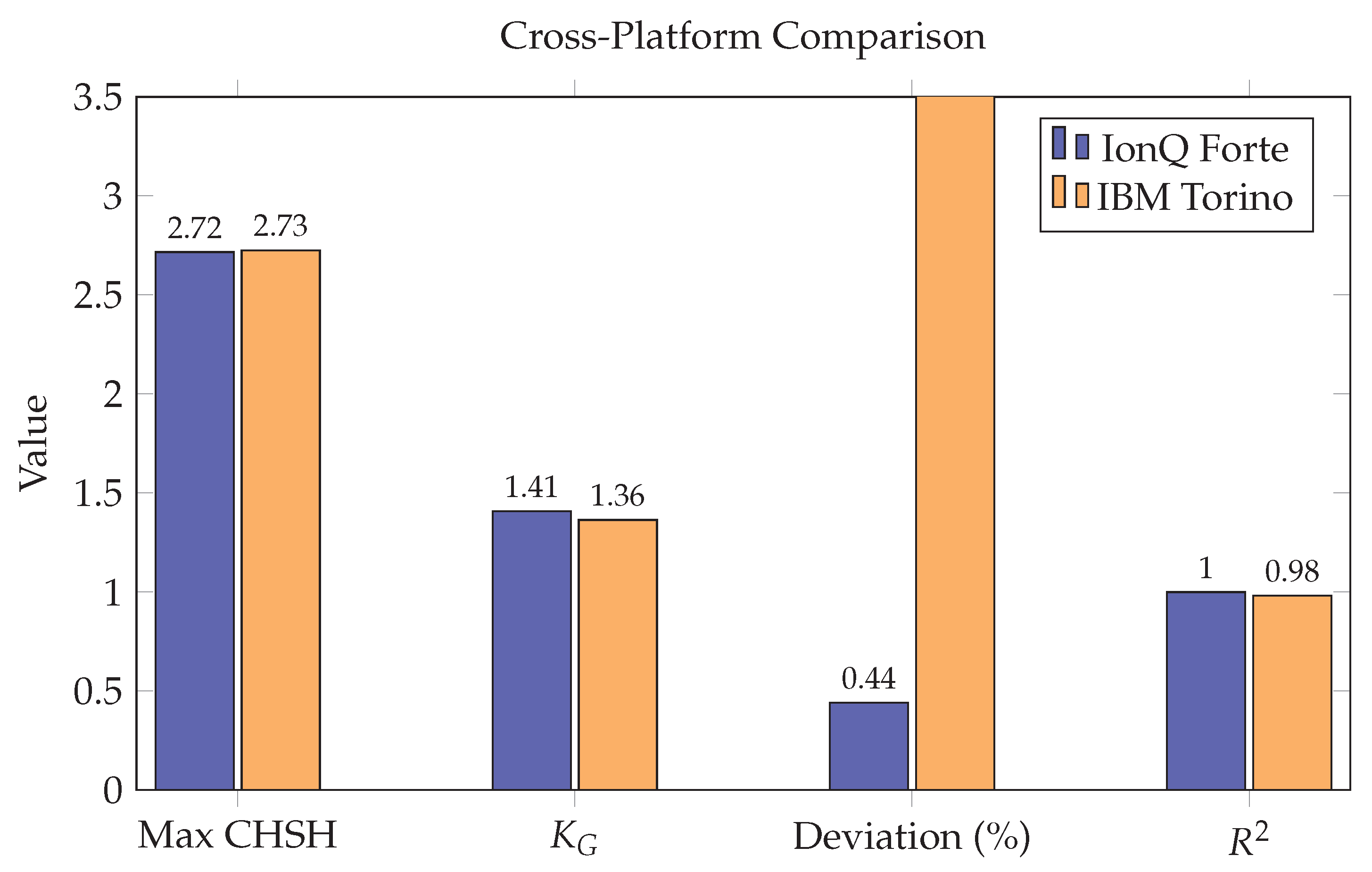

Table 1.
IonQ Forte Enterprise visibility sweep results. Each row represents an independent experiment with visibility controlled via partial entanglement (rotation angle in state preparation). The visibility column shows the achieved value estimated from correlator magnitudes; crucially, extraction uses the slope of S versus v, not the individual visibility estimates, avoiding circularity.
| Run | Visibility | CHSH S | ||||
|---|---|---|---|---|---|---|
| 1 | 0.199 | 0.388 | 0.392 | 0.380 | −0.388 | 1.548 |
| 2 | 0.386 | 0.476 | 0.484 | 0.480 | −0.484 | 1.924 |
| 3 | 0.558 | 0.552 | 0.556 | 0.556 | −0.552 | 2.216 |
| 4 | 0.709 | 0.584 | 0.588 | 0.588 | −0.584 | 2.344 |
| 5 | 0.832 | 0.628 | 0.632 | 0.628 | −0.628 | 2.516 |
| 6 | 0.924 | 0.664 | 0.668 | 0.668 | −0.664 | 2.664 |
| 7 | 0.981 | 0.668 | 0.672 | 0.668 | −0.668 | 2.676 |
| 8 | 1.000 | 0.704 | 0.680 | 0.676 | −0.756 | 2.816 |
Table 2.
Quantitative cross-platform comparison.
| Metric | IBM Torino | IonQ Forte | Ratio/Difference |
|---|---|---|---|
| Maximum CHSH S | 2.725 | 2.816 | 0.968 |
| Tsirelson ratio | 96.4% | 99.6% | 0.968 |
| Extracted | 0.968 | ||
| Deviation from | 3.6% | 0.44% | |
| Regression | 0.9812 | 0.9987 | 0.982 |
| Bell state fidelity | ∼0.90 | 0.984 | 0.915 |
Disclaimer/Publisher’s Note: The statements, opinions and data contained in all publications are solely those of the individual author(s) and contributor(s) and not of MDPI and/or the editor(s). MDPI and/or the editor(s) disclaim responsibility for any injury to people or property resulting from any ideas, methods, instructions or products referred to in the content. |
© 2025 by the author. Licensee MDPI, Basel, Switzerland. This article is an open access article distributed under the terms and conditions of the Creative Commons Attribution (CC BY) license (https://creativecommons.org/licenses/by/4.0/).
Copyright: This open access article is published under a Creative Commons CC BY 4.0 license, which permit the free download, distribution, and reuse, provided that the author and preprint are cited in any reuse.


