Submitted:
01 December 2025
Posted:
03 December 2025
You are already at the latest version
Abstract
Background: Generative Adversarial Networks (GANs) have emerged as powerful tools for medical image synthesis and clinical outcome prediction. In ophthalmology, accurate forecasting of Optical Coherence Tomography (OCT) images and Best Corrected Visual Acuity (BCVA) values can significantly enhance patient monitoring, personalized treatment planning, and early clinical intervention. Methods: We introduce a multimodal GAN framework inspired by StyleGAN architecture, enhanced with super-resolution modules, a multi-scale patch discriminator, and temporal attention mechanisms. For predicting logMAR time series values, we incorporated a hybrid deep-shallow LSTM model, jointly trained alongside the image generation pipeline. After OCT image generation, the synthesized scans were fed into a classification model to predict relevant retinal biomarkers, enabling a com bined structural and functional assessment. Experiments were conducted using the publicly available OLIVES dataset, which contains data from 87 patients and 96 unique eyes, with more than 67,000 OCT images collected from the PRIME and TREX-DME clinical trials. To ensure subject independence between training and testing, we used a patient-level split, assigning 70% of patients to training and 30% to testing. This yields a held-out test set of approximately 26 patients (around 29 eyes), providing a sufficiently large and clinically diverse cohort to make our reported results reliable. Model evaluation was performed using an image similarity-based approach for predicted OCTs, while BCVA (Best Corrected Visual Acuity) and CST (Central Subfield Thickness) predictions were assessed using mean absolute error (MAE), peak signal-to-noise ratio (PSNR), and trend-based categorization of logMAR into improvement, stabilization, or deterioration, with subsequent evaluation via class-wise recall, precision, and F1 scores. Results: The proposed multimodal GAN achieved a Structural Similarity Index (SSIM) of 0.9264, Fréchet inception distance(FID) 11.9 and a Peak Signal-to-Noise Ratio (PSNR) of 38.1 dB for OCT image forecasting, demonstrating superior anatomical fidelity and perceptual quality. The logMARprediction module delivered accurate forecasting performance, with a Mean Absolute Error (MAE) of 0.052 and Mean Squared Error (MSE) of 0.0058, closely aligned with observed clinical outcomes. Conclusions: The developed multimodal GAN approach effectively forecasts future OCT scans, predicts logMAR values, and identifies retinal biomarkers, offering valuable predictive insights into patient trajectories. Such integrative forecasting supports personalized clinical decision-making and proactive disease management in ophthalmology, with potential implications for improving patient outcomes and clinical workflows.
Keywords:
generative adversarial networks
; GAN
; OCT imaging
; logMAR/logMAR forecasting
; ophthalmology
; StyleGAN
; multimodal forecasting
; diabetic retinopathy
1. Introduction
Accurate forecasting of a patient’s future medical condition is a crucial aspect of personalized healthcare, aiding in early intervention and optimized treatment planning [1]. In particular, predicting a patient’s next clinical visit, including generating medical imaging scans, can enhance diagnostic precision and improve patient outcomes. Recent advancements in deep learning, particularly generative models and time-series forecasting techniques, have enabled the possibility of synthesizing future medical scans based on a patient’s historical imaging data.
Traditional forecasting models often rely on regression-based or classification-based approaches. While these methods provide useful insights, they may struggle to capture complex, non-linear patterns inherent in many real-world phenomena. Such limitations can impact predictive accuracy, particularly when dealing with dynamic systems that evolve over time [1]. Time series-based methods, in contrast, analyze sequential data points—either discrete or continuous—to identify trends, patterns, and dependencies over time. By preserving temporal relationships within the data, these models provide a more comprehensive framework for forecasting and decision-making. Advanced deep learning techniques, such as recurrent neural networks (RNNs), long short-term memory (LSTM) networks, and transformer-based architectures, further enhance predictive capabilities by capturing dependencies across longitudinal data [2,3].
Using time series forecasting, it is possible to predict future images based on past observations, enabling applications such as medical imaging progression analysis, weather pattern visualization, satellite image forecasting, and video frame prediction. These models help in identifying subtle changes over time, improving early anomaly detection and long-term planning. One of the most promising approaches in this area is TimeGAN, a generative adversarial network specifically designed for time series data. Unlike traditional GANs, which focus on independent data distributions, TimeGAN preserves temporal dependencies while generating synthetic sequences that closely mimic real data. By leveraging both supervised and unsupervised learning components, TimeGAN can effectively learn the underlying dynamics of sequential data, making it particularly useful for forecasting images where continuity and consistency across time steps are crucial [4,5].
Several studies have implemented time-series GANs on medical imaging data to generate future scans, aiding in disease progression prediction. The Sequence-Aware Diffusion Model (SADM) [6] focuses on longitudinal medical image generation, while Cardiac Aging Synthesis from Cross-Sectional Data with Conditional GANs addresses cardiac MRI scans. GRAPE [7] introduces a multi-modal dataset of longitudinal visual field and fundus images for glaucoma management, and A Deep Learning System for Predicting Time to Progression of Diabetic Retinopathy leverages deep learning for retinal disease forecasting. These works collectively enhance predictive capabilities in brain MRI [8], cardiac MRI [9], and fundus imaging using longitudinal data.
In this research, we propose a novel approach to forecasting a patient’s follow-up scan by leveraging previous visit scans and associated clinical information. Unlike conventional prediction models that focus on classification or segmentation, our method aims to generate synthetic medical scans that accurately reflect anticipated disease progression. To achieve this, we developed MedTimeGAN, a deep generative model that integrates Temporal 3D CNNs, StyleGAN blocks, Super-Resolution, and a Multiscale Patch Discriminator. Additionally, we include a deep-shallow LSTM module to jointly forecast scalar logMAR values. Once the next-visit scan is generated, it is further analyzed using a pretrained EfficientNet-based classification network to predict 16 clinically relevant retinal biomarkers, namely: atrophy/thinning of retinal layers, disruption of the ellipsoid zone (EZ), disorganization of the retinal inner layers (DRIL), intraretinal (IR) hemorrhages, intraretinal hyperreflective foci (IRHRF), partially attached vitreous face (PAVF), fully attached vitreous face (FAVF), preretinal tissue or hemorrhage, vitreous debris (VD), vitreomacular traction (VMT), diffuse retinal thickening/macular edema (DRT/ME), intraretinal fluid (IRF), subretinal fluid (SRF), disruption of the retinal pigment epithelium (RPE disruption), serous pigment epithelial detachment (Serous PED), and subretinal hyperreflective material (SHRM). By incorporating longitudinal patient data, our approach provides a robust and unified framework for clinical decision-making, offering insights into disease evolution and assisting healthcare professionals in personalized treatment planning.
2. Dataset
The Ophthalmic Labels for Investigating Visual Eye Semantics (OLIVES) dataset [10] is a comprehensive, multi-modal ophthalmic resource curated for machine learning research in disease progression modeling, diagnosis, and treatment planning. It contains longitudinal data from 96 eyes (patients), followed over an average of 66 weeks and 16 clinic visits. The dataset integrates scalar clinical labels—Best Corrected Visual Acuity (BCVA) and Central Subfield Thickness (CST)—alongside expert-annotated vector biomarkers, two-dimensional near-infrared (NIR) fundus images, and three-dimensional Optical Coherence Tomography (OCT) scans.

Table 1.
Detailed Modality Breakdown and Annotations in the OLIVES Dataset. Here, represents the number of visits per patient (on average, 16 visits per eye).
Table 1.
Detailed Modality Breakdown and Annotations in the OLIVES Dataset. Here, represents the number of visits per patient (on average, 16 visits per eye).
| Modality | Per Visit | Per Eye | Total | Type | Notes |
|---|---|---|---|---|---|
| OCT (3D) | 49 B-scans | 78,189 | 3D volume | 49 B-scans per visit; = #visits/patient | |
| Fundus (NIR) | 1 | 1,268 | 2D image | Near-infrared fundus photographs | |
| Clinical Labels | 4 | 5,072 | Tabular | BCVA, CST, Patient/Eye ID per visit | |
| Biomarkers | 16 | 16 | 9,408 | Vector | Annotated for first and last visits |
| Disease Label | 1 | 96 | Category | DR or DME per eye | |
| Time Series | — | ∼16 | Longitudinal | Mixed | ∼16 visits over 2 years, with 7 injections |
To support temporal forecasting tasks, only eyes with at least ten valid visits were retained. Scalar BCVA values were originally provided in ETDRS letters but were converted into logarithm of the minimum angle of resolution (logMAR) units using the standard ETDRS formula [11]:
where higher logMAR values indicate worse visual acuity. Together with CST, these values were normalized to the range and organized into visit-aligned sequences ( to ). A sliding window strategy was applied to create overlapping sequences for supervised learning (e.g., , , →), resulting in 672 valid training samples. To enhance temporal pattern learning, we applied Daubechies-4 (db4) wavelet decomposition [12] at level 3 to each logMAR series, capturing both trend and detail coefficients.
OCT volumes from each visit consist of 49 B-scans, which were resized to pixels and z-score normalized using training set statistics. For temporal prediction, pairs of previous OCT volumes (e.g., , ) were used to forecast the next volume (). The central slice (25th B-scan) was used for qualitative evaluation and visual comparison against ground truth.
We implemented a custom PyTorch Dataset class to facilitate training. It groups B-scans by (Patient_ID, Visit), applies preprocessing and transforms, and constructs sequences of 48 B-scans. If a visit contains fewer than 48 images, zero-padding is applied; excess images are truncated. Each sample is represented as a 4D tensor of shape . Missing or unreadable images are replaced with zero-valued tensors to maintain consistency.
For multimodal experiments, CST and logMAR values per visit are either used as regression targets or incorporated as conditioning features. CST, which reflects macular thickness, enhances the model’s ability to learn anatomical context relevant to functional vision outcomes. To ensure robust evaluation and prevent temporal or identity leakage, a 3-fold cross-validation split was applied at the patient level. Each fold contains a disjoint set of patients, maintaining temporal integrity within each fold to simulate real-world longitudinal forecasting scenarios.
The OLIVES dataset is publicly available for academic research and can be accessed at https://zenodo.org/records/7105232.
3. Multimodal Architecture
Our proposed framework is designed for time series image forecasting, super-resolution, biomarker prediction, and clinical outcome forecasting. It draws inspiration from StyleGAN and modern adversarial learning techniques. The architecture consists of four jointly trained components: (1) a StyleGAN-based generator for synthesizing future OCT frames, (2) a multi-scale PatchGAN discriminator for enforcing spatial realism, (3) an EfficientNet-B0 classifier for predicting disease-relevant biomarkers from generated OCT frames, and (4) a DeepShallow LSTM module for ogMAR from historical An overview is illustrated in Figure 1.
3.1. StyleGAN Generator
The generator adopts a StyleGAN-inspired encoder-decoder design tailored for spatiotemporal medical time series forecasting. It takes as input a sequence of T grayscale frames (e.g., historical OCT scans) and outputs a super-resolved prediction of the next frame.
Spatial-Temporal Encoding
Each frame in the input sequence is encoded via a shared convolutional encoder with stacked convolutions and LeakyReLU activations. This abstracts spatial features and projects each frame to a latent embedding. The temporal stack of latent vectors is aggregated to model progression dynamics.
Contextual Modeling with StyleGAN Blocks
The temporal features are processed through a series of StyleGAN-inspired residual blocks consisting of convolutions, instance normalization, and skip connections. These blocks model contextual dependencies and provide robust spatiotemporal representations.
Decoding and Super-Resolution
The encoded sequence is decoded using a series of transposed convolutions, which progressively upsample the features. A dedicated super-resolution head further enhances the spatial fidelity, restoring high-frequency details. The final output is a single normalized frame at resolution.
3.2. Multi-Scale PatchGAN Discriminator
To assess the realism of generated frames, we employ a multi-scale PatchGAN discriminator operating at two spatial resolutions:
Patch-Based Supervision
Each discriminator receives a concatenation of the historical input frame and either the real or generated next frame. At full scale () and half scale (), patch-level discrimination encourages local realism and structural consistency.
Adversarial Optimization
The outputs from each scale are averaged to form the total adversarial loss:
pushing the generator to produce visually plausible and anatomically accurate frames.
3.3. logMAR Forecasting via DeepShallow LSTM
To jointly predict clinical outcomes, we integrate a DeepShallow LSTM model that consumes both structured clinical data and visual embeddings to forecast future logMAR scores.
Multimodal Input Representation
The input to the LSTM model is a multivariate time series composed of three elements:
(1) historical Best Corrected Visual Acuity (logMAR),
(2) central subfield thickness (CST), and
(3) visual latent features extracted from the generator’s encoder.
These components are concatenated per visit, forming the multimodal input tensor:
where T is the number of historical visits, the scalar features (logMAR, CST) contribute 2 dimensions, and d denotes the encoder’s latent embedding dimension.
Temporal Regression
A two-layer LSTM with hidden size 64 captures disease progression patterns across visits. The final hidden state is passed through a fully connected regressor:
to generate the predicted logMAR value at the next timepoint.
This multimodal formulation enables the model to learn complex interactions between anatomical features, prior visual outcomes, and imaging-based representations.
3.4. Training Objective
The full model is optimized end-to-end using a composite objective that integrates adversarial learning, reconstruction fidelity, spatial smoothness, and clinical regression accuracy:
where:
- : adversarial loss from multi-scale PatchGAN discriminators,
- : pixel-wise or perceptual reconstruction loss (e.g., or VGG loss) between predicted and ground truth frames,
- : total variation loss that encourages smoothness and reduces artifacts in the generated image,
- : clinical regression loss that penalizes errors in logMAR forecast. Defined as:where is the predicted score and is the ground truth.
The weights are tuned empirically to balance visual fidelity and clinical outcome accuracy. In our experiments, we found that , , , and yielded optimal trade-offs across validation metrics.
3.5. Training Strategy
To model disease progression over time and forecast both future OCT scans and logMAR values, we adopt a sliding window strategy across longitudinal visit data for each patient. The dataset provides up to 10 timepoints per eye, labeled from to . From these, we construct temporal training samples using overlapping pairs and triplets of historical visits to predict subsequent visits.
For example, using 2-visit inputs, we form training samples such as , , and so on up to . Similarly, for 3-visit inputs, we generate sequences such as , ..., . These samples are stacked across the dataset to form a rich set of temporally coherent training examples.
Each input window includes full 3D OCT volumes from 49 B-scans per visit, resized to resolution. These volumes are processed by the generator to synthesize the future visit’s B-scans. For logMAR prediction, a separate LSTM-based regression head consumes the same historical window to forecast the scalar logMAR value corresponding to the predicted scan.
During training, we ensure that the prediction target is never included in the input window to avoid temporal leakage. The model is trained in a teacher-forcing mode, where each prediction is made independently based on previous ground truth visits. This design supports both single-step forecasting during training and autoregressive inference during evaluation.
To improve robustness, we aggregate training samples from all available patient trajectories, padding sequences where fewer than 10 visits exist. The total training set thus captures a wide range of disease stages, injection events, and recovery patterns across multiple time horizons.
3.6. Training and Loss Functions
The model is trained within a conditional adversarial learning framework, where the generator and discriminator are jointly optimized to produce high-fidelity, perceptually realistic future frames from spatiotemporal image sequences. Training alternates between updating the generator and discriminator, enabling adversarial feedback to continually refine output realism and anatomical accuracy.
3.6.1. Generator Objectives
The generator is supervised with a composite objective combining adversarial, pixel-wise, perceptual, and structural similarity terms. The adversarial loss compels the generator to produce outputs that the discriminator cannot distinguish from ground truth images, while the pixel-wise reconstruction loss, computed as the L1 distance between generated and real frames, ensures accurate spatial alignment. To further improve perceptual quality, a perceptual loss based on VGG16 feature activations is incorporated, guiding the generator to reconstruct high-level content and texture statistics. Additionally, a structural similarity (SSIM) loss is used to preserve local structure and fine details.
The final generator loss is a weighted sum:
where , , and control the balance between objectives. In our experiments, we set , , and to encourage spatial accuracy, perceptual fidelity, and structural realism.
3.6.2. Discriminator Training
The discriminator is trained to classify real versus synthesized image pairs using a binary cross-entropy loss. To improve stability and enforce smoothness in the discriminator’s output, a gradient penalty term is added. This regularization encourages the gradients of the discriminator with respect to its input to have unit norm, mitigating mode collapse and improving convergence.
The discriminator loss is defined as:
where is the gradient penalty weight (set to 10 in our implementation).
3.6.3. Biomarker Classification Training
In addition to forecasting OCT scans and logMAR values, the generated OCT frames are analyzed using a pretrained EfficientNet-B0 classifier to predict 16 clinically relevant retinal biomarkers. The classifier was trained on the OLIVES dataset, which provides expert-annotated labels for biomarker presence across patient visits. The set of predicted biomarkers includes: atrophy/thinning of retinal layers, disruption of the ellipsoid zone (EZ), disorganization of the retinal inner layers (DRIL), intraretinal (IR) hemorrhages, intraretinal hyperreflective foci (IRHRF), partially attached vitreous face (PAVF), fully attached vitreous face (FAVF), preretinal tissue or hemorrhage, vitreous debris (VD), vitreomacular traction (VMT), diffuse retinal thickening/macular edema (DRT/ME), intraretinal fluid (IRF), subretinal fluid (SRF), disruption of the retinal pigment epithelium (RPE disruption), serous pigment epithelial detachment (Serous PED), and subretinal hyperreflective material (SHRM).
To address the significant class imbalance among biomarkers, the classifier is optimized using focal loss, which down-weights easy negatives and emphasizes harder, underrepresented cases. The focal loss is defined as:
where is the predicted probability of the true class, is a class-balancing weight, and is the focusing parameter (set to 2 in our experiments). This formulation mitigates the dominance of majority classes and improves sensitivity for rare biomarkers.
3.6.4. Optimization Strategy
Both networks are optimized using the Adam optimizer. The generator uses a learning rate of , while the discriminator uses , with momentum parameters and . To enhance stability and avoid stagnation, we employ a step-based learning rate scheduler, halving the learning rate every 20 epochs for both networks.
At each iteration, the discriminator is updated twice per generator step to maintain balance between the networks. Training proceeds for 50 epochs, and performance is monitored using PSNR and SSIM metrics on the validation set. For biomarker classification, the EfficientNet model is trained jointly with the generator outputs and evaluated every epoch using F1 score.
All loss weights, hyperparameters, and optimization routines are tuned to maximize output fidelity, anatomical consistency, and biomarker detection accuracy across diverse validation cases.
3.6.5. Training Infrastructure and Runtime
All models are trained on NVIDIA H100 GPUs provided by the National High-Performance Computing Center (NHR) at TU Dresden. The multimodal model, which integrates OCT image sequences and clinical outcome data (logMAR), requires approximately 32 minutes per epoch due to its increased architectural and input complexity. In contrast, the image-only models take around 25 minutes per epoch.
Each model is trained for 50 epochs using mixed precision to accelerate computation and reduce memory usage. As noted in Table 2, the final two rows correspond to multimodal models, while the remaining rows represent image-only baselines.
To ensure reproducibility and efficient resource utilization, we employ fixed random seeds, deterministic data loaders, and automated logging of performance metrics including PSNR, SSIM, and F1 score on the validation set.
3.6.6. Evaluation Metrics
To quantitatively assess performance, we compute the following metrics during training:
- Peak Signal-to-Noise Ratio (PSNR): Captures the signal fidelity between generated and ground truth OCT outputs. Higher PSNR correlates with lower pixel-wise reconstruction error.
- Structural Similarity Index Measure (SSIM): Evaluates structural integrity, contrast preservation, and perceptual quality. SSIM is particularly sensitive to spatial distortions and is more aligned with human visual perception than pixel-wise metrics.
- F1 Score (macro-averaged): Used to evaluate biomarker classification performance across the 16 predicted categories. This metric balances precision and recall and ensures that less frequent biomarkers are weighted equally in the overall evaluation.
4. Results
This section comprehensively evaluates the proposed multimodal forecasting framework across anatomical, functional, and clinical dimensions. Experiments were performed on longitudinal OCT sequences with corresponding visual acuity (logMAR) measurements. The objective was to assess the model’s capability to forecast future retinal morphology and functional trends from prior visits.
Results are organized into five parts: (1) qualitative visualization of OCT forecasts; (2) quantitative analysis of logMAR trend prediction using the Winner–Stabilizer–Loser framework; (3) model comparison and ablation analysis of generators, discriminators, and loss functions; (4) multimodal biomarker classification from predicted OCTs; and (5) benchmarking against prior longitudinal forecasting methods.
Overall, the proposed model demonstrates three key properties:
- High anatomical fidelity, with predicted OCT frames achieving SSIM up to 0.93 and PSNR exceeding 38 dB,
- Clinically consistent functional forecasting, with logMAR errors (MAE = 0.052) well within the accepted clinical tolerance,
- Trend-awareness, as the model accurately identifies whether a patient’s visual function is improving, stable, or declining across visits.
These results collectively establish that the proposed multimodal GAN learns both spatial structure and temporal dynamics, producing anatomically realistic and clinically interpretable forecasts suitable for longitudinal disease monitoring.
4.1. Qualitative OCT Forecasting Performance
Figure 2 (top) and Figure 3 (top) present qualitative OCT forecasting results for two representative patients (IDs 232 and 234). In both examples, the model receives two consecutive OCT scans (V1 and V2) and predicts the subsequent visit (V3). The predicted frames exhibit high visual fidelity and strong anatomical consistency with the ground truth. Specifically, the forecasts demonstrate:
- Preservation of retinal layer continuity, particularly around the foveal pit and outer retinal boundaries,
- Accurate modeling of macular thickness and edema progression, critical biomarkers for diabetic macular edema (DME) and age-related macular degeneration (AMD),
- Retention of fine microstructural features, facilitated by the super-resolution and StyleGAN-inspired upsampling mechanisms in the generator network.
These results confirm that the proposed model effectively learns spatial and temporal correlations within the retinal morphology, capturing both local structural changes and global thickness variations across visits. Subtle pathological signatures, such as localized depressions and intra-retinal cystic spaces, are preserved in the predicted frames, demonstrating the model’s capacity to generalize across disease stages and longitudinal follow-ups.
These results confirm that the model effectively captures spatio-temporal dependencies in OCT morphology. Moreover, subtle pathological features such as retinal bulges and depressions are maintained in the generated frames, supporting potential application in longitudinal disease monitoring.
4.2. Forecasting Functional Outcome (logMAR)
The lower panels of Figure 2 and Figure 3 illustrate sliding-window forecasts of logMAR trajectories for Patients 232 and 234. Each subplot represents a temporal triplet , where:
- gray circles indicate ground-truth logMAR values at and ,
- Colored markers show the model’s forecast at using a colorblind-safe palette,
- Cross-shaped “×” markers indicate the ground-truth logMAR at , colored with the same class color for direct comparison.
Predicted outcomes are categorized using the deviation between prediction and the previous visit:
- Winner (): predicted improvement in visual acuity (lower logMAR),
- Stabilizer (): predicted stable visual acuity,
- Loser (): predicted deterioration (higher logMAR).
Patient 232 (Figure 2): Across nine temporal windows, the model successfully tracks logMAR evolution and the overall disease trend.
- In the V1,V2 → V3 window, the model’s numerical estimate is slightly higher than the true logMAR deterioration (0.58 vs. 0.54), but it still correctly assigns the Loser class.
- In the V2,V3 → V4 window, the prediction matches the ground truth (0.28), indicating a Winner.
- In later visits, e.g., V5,V6 → V7, the prediction (0.32) equals GT (0.32), representing a Stabilizer.
This consistency across sequential visits highlights that the model not only produces accurate logMAR values but also respects the directionality of visual function changes, correctly identifying improvement, stability, or decline phases.
Patient 234 (Figure 3): For this patient, logMAR values fall within the negative range (reflecting higher visual acuity). The model effectively captures improvement and stabilization trends:
- In the early V1, V2 → V3 window, the forecast () closely matches GT (), denoting a Winner.
- In V2, V3 → V4, the model output () stays within of GT (), resulting in a Stabilizer.
- In later windows (e.g., V8, V9 → V10), the model predicts vs. GT , again falling into the Stabilizer range.
Across visits, predictions remain well within clinical tolerance thresholds (), demonstrating robustness even when logMAR reversals or subtle fluctuations occur.
Summary: The results demonstrate that the model does not merely perform pointwise regression but learns the underlying temporal behavior of visual function. The Winner–Stabilizer–Loser classification framework provides an interpretable means to assess prediction reliability and trend consistency:
- Winners correspond to predicted improvements, highlighting recovery tendencies,
- Stabilizers dominate across visits, showing that the model can maintain disease stability over time,
- Losers appear infrequently and usually represent small deviations within the noise margin of measurement error.
By correctly identifying the temporal direction of change, the model demonstrates strong potential for trend-aware visual prognosis, enabling longitudinal interpretation of patient recovery or decline.
4.3. Winner–Stabilizer–Loser Classification Across Thresholds
Table 3 presents the distribution of Winner, Stabilizer, and Loser outcomes for four patients (IDs 201, 203, 232, and 234) across varying tolerance thresholds (–). Lower values represent strict thresholds (minor deviations are penalized), while higher values allow greater clinical tolerance.
- Patient 201: Shows balanced outcomes at but converges to entirely stable predictions by , with no Losers remaining.
- Patient 232: Initially sensitive to small fluctuations (13 Losers at ), yet transitions fully to Stabilizers beyond , demonstrating consistency under realistic tolerances.
- Patient 234: Exhibits steady improvement; Losers diminish progressively, and all predictions become Stabilizers by .
- Patient 236: Displays early variability but stabilizes completely by , mirroring trends in Patient 232.
This trend-based interpretation highlights that the model adapts well across patients and tolerance levels, consistently maintaining temporal coherence in visual function forecasting.
4.4. Confusion Matrix Evaluation at
The confusion matrices shown in Figure 4 and Figure 5 summarize the agreement between the model’s predicted trajectory classes and the ground-truth delta-based labels for each patient. Each matrix compares three clinically relevant progression categories:
- Winner (W): Improvement beyond the negative threshold (),
- Stabilizer (S): Minimal change within the threshold range (),
- Loser (L): Worsening beyond the positive threshold ().
Correct predictions appear along the diagonal of each matrix, whereas off-diagonal values represent misclassifications. A higher concentration of values along the diagonal therefore indicates stronger predictive accuracy. The overall confusion matrix exhibits a clear diagonal dominance, demonstrating that the model reliably differentiates between improving (W), stable (S), and worsening (L) trajectories across all patients.
Individual patient confusion matrices reveal patient-specific performance patterns. Patients 201, 203, and 232 show strong diagonal structures with minimal misclassification, indicating highly predictable progression patterns. Patient 204 displays more variability, with a larger number of S-to-L confusions, suggesting more complex or borderline changes around the threshold.
A detailed quantitative summary of precision, recall, and F1-scores for the overall dataset and each patient is provided in Table 4. These metrics reinforce the visual observations from the confusion matrices and confirm that the model performs consistently across most patients, with only minor deviations in more challenging cases.
4.5. Quantitative Results and Model Comparison
Table 2 presents a comprehensive evaluation of multiple generator–discriminator configurations, input sequence lengths, loss formulations, and training strategies for OCT time-series forecasting. IDs 1–4 correspond to baseline configurations trained for 250 epochs, including earlier Transformer-based and Temporal-CNN baselines (IDs 1–2) and an initial version of Generator 1 (IDs 3–4). From ID 5 onward, all models are trained for 350 epochs, which includes the full Generator 1 + Discriminator 1 pipeline (IDs 5–12) as well as the multimodal models (IDs 13–14).
IDs 5–12 employ Generator 1 (Temporal CNN + Super-Resolution + StyleGAN-inspired blocks) with Discriminator 1 (multi-scale patch discriminator). IDs 13–14 use Generator 2, an extended architecture that integrates temporal cross-frame attention to jointly predict future OCT frames and logMAR visual acuity.
Performance metrics include SSIM and PSNR for image quality, FID for distributional fidelity, and MAE/MSE for the multimodal logMAR prediction. The experiments use different loss formulations: Loss_1 (BCE+Perceptual), Loss_2 (BCE+GP+Perceptual+Pixel+Adversarial+SSIM), and Loss_3 (BCE+Wasserstein+GP+Perceptual+Pixel+Adversarial+SSIM).
The best overall performance is achieved by the multimodal temporal-attention model (ID 14), trained for 350 epochs, reaching SSIM 0.9264 and PSNR 38.1.
- SSIM: Measures perceptual and structural similarity between predicted and ground truth OCT images.
- PSNR: Reflects pixel-level fidelity and noise robustness.
- MAE and MSE: Capture absolute and squared errors in logMAR prediction (only applicable in multimodal models).
Baseline Performance:
A Transformer-based model with positional encoding and perceptual loss (row 1) yields poor visual quality (SSIM = 0.5432, PSNR = 0.1314), underscoring the limitations of using only static image encoding and no temporal modeling.
Effect of Temporal Modeling and StyleGAN Blocks:
Introducing temporal CNNs and super-resolution modules (Generator_1) markedly improves performance. For example:
- v1, v2 → v3 improves to SSIM = 0.7938, PSNR = 0.2931,
- v1, v2, v3, v4 → v5 achieves SSIM = 0.8611, indicating the benefit of longer temporal windows.
Multimodal Forecasting with Generator_2:
We began our experiments with a baseline generator architecture (Models ID 1–4), establishing reference performance for single-visit and simple paired-input forecasting. Building on these results, we adopted the enhanced Generator_2 design with temporal attention and multimodal fusion. This model was evaluated using 2-pair, 3-pair, and 4-pair input sequences to predict the next OCT frame and its corresponding logMAR value.
Due to dataset limitations—specifically the inconsistency of longer longitudinal sequences—we focused on the most reliable configurations: 2-pair and 3-pair inputs. Among all tested settings, the 3-pair multimodal configuration produced the best overall performance, as summarized in Table 2.
The final Generator_2 model (3-pair input) achieves:
- SSIM = 0.9264, PSNR = 0.4169,
- MAE = 0.052, MSE = 0.0058.
These results confirm the synergy of multimodal learning and dynamic attention-driven temporal encoding. The improved logMAR prediction further highlights the model’s ability to forecast functional vision outcomes alongside structural OCT progression, even with limited longitudinal data.
4.6. Biomarker Classification Results
In addition to anatomical and functional forecasting, our multimodal framework predicts 16 clinically relevant retinal biomarkers from the generated OCT scans using a pretrained EfficientNet-B0 multilabel classifier. The predicted biomarkers include: atrophy/thinning of retinal layers, disruption of the ellipsoid zone (EZ), disorganization of the retinal inner layers (DRIL), intraretinal hemorrhages (IR), intraretinal hyperreflective foci (IRHRF), partially attached vitreous face (PAVF), fully attached vitreous face (FAVF), preretinal tissue or hemorrhage, vitreous debris (VD), vitreomacular traction (VMT), diffuse retinal thickening/macular edema (DRT/ME), intraretinal fluid (IRF), subretinal fluid (SRF), disruption of the retinal pigment epithelium (RPE disruption), serous pigment epithelial detachment (Serous PED), and subretinal hyperreflective material (SHRM).
Quantitative evaluation on the OLIVES dataset demonstrates strong performance despite class imbalance. Using focal loss during training, the classifier achieved a macro-averaged F1 score of 0.81, with per-class F1 scores ranging from 0.72 (IR hemorrhages) to 0.89 (subretinal fluid).
Table 5 provides detailed precision, recall, and F1 scores for each biomarker.
4.7. Comparison with Prior Longitudinal Forecasting Models
Several prior studies have explored generative and predictive modeling of disease progression using longitudinal medical data. Notably, the Sequence-Aware Diffusion Model (SADM) [6] and the GRAPE dataset [7] serve as representative efforts in volumetric image generation and functional outcome prediction, respectively. In this section, we highlight how our proposed multimodal GAN framework advances beyond these approaches in terms of forecasting capacity, multimodal fusion, and clinical utility.
Comparison with SADM
SADM [6] uses a diffusion model with transformer-based attention modules to model temporal dependencies in longitudinal 3D medical scans such as cardiac and brain MRI. The method supports autoregressive sampling and handles missing frames through zero tensor masking. While SADM shows strong performance (e.g., SSIM = 0.851 on cardiac MRI), it requires significant compute resources and does not support scalar outcome prediction. In contrast, our method achieves higher structural fidelity (SSIM = 0.9264), incorporates super-resolution modules, and jointly forecasts both anatomical (OCT) and functional (logMAR) trajectories. Moreover, our GAN-based approach provides faster convergence and inference than diffusion models, making it more suitable for clinical integration.
Comparison with GRAPE
GRAPE [7] presents a longitudinal multimodal dataset of glaucoma patients, including color fundus photographs (CFPs), OCT, and visual field (VF) tests. It focuses primarily on VF progression prediction via deep learning models such as ResNet-50, achieving AUCs of 0.71–0.80 depending on the criterion. However, GRAPE does not generate future anatomical images nor integrate time-series modeling. In contrast, our framework models dynamic imaging and scalar progression jointly using longitudinal OCT scans and logMAR time series, capturing both structural and functional evolution over time.
Summary
Our multimodal GAN approach introduces a novel integration of spatiotemporal generation and clinical forecasting. By combining StyleGAN blocks, temporal attention, and a DeepShallow LSTM, our model offers both fine-grained anatomical realism and accurate clinical predictions, surpassing the scope of prior methods.
Table 6.
Comparison of our multimodal GAN approach with prior methods and datasets. Our method uniquely combines anatomical frame forecasting with functional scalar prediction in an end-to-end fashion.
Table 6.
Comparison of our multimodal GAN approach with prior methods and datasets. Our method uniquely combines anatomical frame forecasting with functional scalar prediction in an end-to-end fashion.
| Model / Dataset | Modality | Input | Output | Architecture | Forecast Task | Metrics |
|---|---|---|---|---|---|---|
| Our Model | OCT + logMAR | V1–V3 OCT + logMAR | V4 OCT + logMAR | StyleGAN + LSTM + SuperRes | Imaging + Scalar Regression | SSIM 0.9264, MAE 0.052 |
| SADM [6] | Brain/Cardiac MRI | ED + frames (3D) | Future MRI frame | Diffusion + Transformer | Imaging (Autoregressive) | SSIM 0.851, PSNR 28.99 |
| GRAPE [7] | CFP, OCT, VF | Baseline CFP/OCT | VF Progression Class | ResNet-50 | VF Classification (PLR/MD) | AUC 0.71–0.80, MAE 4.14 |
4.8. Loss Function Ablation
The loss functions used in generator training significantly affect outcome quality:
- Loss_1 (BCE + perceptual loss): Produces sharp but occasionally unstable predictions.
- Loss_2 (adds gradient penalty, SSIM, pixel-wise terms): Yields improved convergence and sharper details.
- Loss_3 (adds Wasserstein term): Stabilizes adversarial training and maximizes perceptual quality.
Overall, Loss_3 in combination with Generator_2 produces the highest visual and functional fidelity.
5. Discussion
This study introduces a multimodal generative forecasting framework capable of predicting future OCT anatomy, visual acuity (logMAR), and biomarker evolution using longitudinal ophthalmic data. By integrating temporal attention, StyleGAN-inspired blocks, super-resolution modules, and a DeepShallow LSTM, the model jointly captures both structural and functional disease progression. The results demonstrate that this multimodal formulation substantially outperforms image-only and scalar-only baselines, underscoring the value of combining imaging and clinical time-series information for ophthalmic prognosis.
5.1. Interpretation of Anatomical and Functional Forecasting
The proposed architecture achieves high-fidelity anatomical predictions, with SSIM values reaching 0.9264 and PSNR exceeding 38 dB. These metrics indicate that the model effectively preserves retinal layer continuity, foveal contour, and fluid-related microstructures—elements that are essential for monitoring diabetic macular edema (DME) and other retinal diseases. The incorporation of temporal attention enables the model to prioritize the most diagnostically informative visits, improving its ability to reconstruct subtle disease trajectories and distinguishing it from conventional recurrent or convolutional temporal encoders.
The multimodal logMAR forecasting component also performs strongly, achieving a mean absolute error (MAE) of 0.052, which is well within the typical logMAR test–retest variability. Importantly, the forecasts do not simply regress toward mean values; instead, they maintain the directionality of visual function changes across visits. Using the Winner–Stabilizer–Loser framework, the model demonstrates robust trend-aware predictions, aligning with clinically observed improvements, stabilizations, and deteriorations.
5.2. Comparison With Prior Longitudinal Imaging Models
Compared to diffusion-based approaches such as SADM, which achieves SSIM values around 0.85 on cardiac MRI, the proposed GAN-based framework offers superior structural fidelity while enabling faster training and inference. Models associated with the GRAPE dataset primarily focus on visual field progression without generating future anatomical images, whereas our method jointly synthesizes future OCT frames and functional outcomes, providing a more comprehensive understanding of disease evolution.
The combination of StyleGAN blocks, super-resolution modules, and adversarial supervision is particularly effective for ophthalmic imaging, where fine structural details and layer boundaries must be preserved. By contrast, transformer-only or CNN-only baselines in earlier experiments produce lower SSIM and PSNR values, highlighting the importance of the proposed multimodal temporal architecture.
5.3. Clinical Relevance
The forecasting capability of the model has direct clinical implications:
- Proactive monitoring: Predicting OCT structural changes in advance enables earlier detection of disease progression.
- Personalized therapy planning: Forecasted OCT and logMAR trajectories offer insights into expected responses to treatment, particularly anti-VEGF regimens.
- Digital retinal twins: The model supports individualized longitudinal simulations, enhancing population-level modeling and clinical trial design.
The strong biomarker detection performance on generated OCTs (macro-F1 = 0.81) further validates the anatomical realism of the synthesized images. These findings support the utility of such models in decision-support systems for retinal disease management.
5.4. Limitations
Several limitations should be considered:
- The OLIVES dataset, although rich in longitudinal information, includes only 96 eyes, which is modest for training deep generative models.
- Qualitative assessment was centered on the middle B-scan; full 3D volumetric evaluation remains to be explored.
- Biomarker annotations are available only for the first and last visits, limiting longitudinal biomarker supervision.
- Treatment events (e.g., anti-VEGF injections) are not explicitly encoded, despite their influence on disease trajectories.
- Multi-step autoregressive rollouts may accumulate error over longer prediction horizons.
Addressing these limitations will enhance generalizability and support deployment in clinical environments.
5.5. Future Work
Future research directions include:
- Extending the generator to full 3D volumetric OCT forecasting.
- Incorporating treatment history and dosage to enable treatment-aware forecasting.
- Exploring hybrid GAN–diffusion frameworks to improve global coherence and detail preservation.
- Applying interpretability tools such as attention visualization and saliency maps.
- Cross-dataset validation on additional longitudinal ophthalmic datasets to assess generalizability.
- While the present analysis did not focus on temporal treatment dynamics, future studies should incorporate time-dependent effects associated with the three dosing regimens (fixed, PRN (pro re nata, (if needed)), and treat-and-extend) to more fully capture their differential impact on therapeutic outcomes.
- Future research should also directly compare the temporal effectiveness of anti-VEGF therapy with corticosteroid-based treatments to clarify their relative benefits across different disease activity patterns and patient subgroups.
To advance the field, we encourage the medical community to generate and share similarly detailed real-world datasets—beyond those currently available in the OLIVES dataset—to enable more comprehensive analyses of treatment patterns, temporal effects, and comparative outcomes across therapeutic regimens.
Acknowledgments
This research was partially funded by the European Social Fund for Germany and the Federal Ministry of Education and Research (BMBF) through the Medical Informatics Hub in Saxony (MiHUBx) under grant number 01ZZ2101C. Computational resources were provided by the National High Performance Computing (NHR) Center at TU Dresden. The NHR centers are jointly supported by the German Federal Government and the state governments participating in the NHR alliance. We gratefully acknowledge their GPU infrastructure, which enabled large-scale model training and experimentation.
Abbreviations
The following abbreviations are used in this manuscript:
| CST | Central Subfield Thickness |
| logMAR | Best Central Visual Acuity |
| Eye ID | Eye Identity |
| EZ | Ellipsoid Zone |
| DRIL | Disruption of the Retinal Inner Layers |
| IR | Intraretinal |
| IRHRF | Intraretinal Hyperreflective Foci |
| PAVF | Partially Attached Vitreous Face |
| FAVF | Fully Attached Vitreous Face |
| VMT | Vitreomacular Traction |
| DRT/ME | Diffuse Retinal Thickening or Macular Edema |
| IRF | Intraretinal Fluid |
| SRF | Subretinal Fluid |
| RPE | Retinal Pigment Epithelium |
| PED | Pigment Epithelial Detachment |
| SHRM | Subretinal Hyperreflective Material |
| DR | Diabetic Retinopathy |
| DME | Diabetic Macular Edema |
| CI-DME | Center-Involved Diabetic Macular Edema |
| PDR | Proliferative Diabetic Retinopathy |
| NPDR | Non-Proliferative Diabetic Retinopathy |
| OCT | Optical Coherence Tomography |
| AMD | Age-related Macular Degeneration |
| CNV | Choroidal Neovascularization |
| VEGF | Vascular Endothelial Growth Factor |
| ETDRS | Early Treatment Diabetic Retinopathy Study |
| OLIVES | Ophthalmic Labels for Investigating Visual Eye Semantics |
| FID | Fréchet inception distance |
References
- Kong, X.; Chen, Z.; Liu, W.; Ning, K.; Zhang, L.; Marier, S.M.; Liu, Y.; Chen, Y.; Xia, F. Deep learning for time series forecasting: A survey. Int. J. Mach. Learn. Cybern. 2025, 10, 1–25. [Google Scholar] [CrossRef]
- Hamilton, J.D. Time Series Analysis; Princeton University Press: Princeton, NJ, USA, 1994. [Google Scholar]
- Montgomery, D.C.; Jennings, C.L.; Kulahci, M. Introduction to Time Series Analysis and Forecasting, 2nd ed.; John Wiley & Sons: Hoboken, NJ, USA, 2015. [Google Scholar]
- Yoon, J.; Jarrett, D.; van der Schaar, M. Time-series generative adversarial networks. In Advances in Neural Information Processing Systems (NeurIPS 2019); Curran Associates, Inc.: Red Hook, NY, USA, 2019; Volume 32, pp. 5508–5518. [Google Scholar]
- EskandariNasab, M.; Hamdi, S.M.; Filali Boubrahimi, S. SeriesGAN: Time series generation via adversarial and autoregressive learning. Pattern Recognit. Lett. 2023, 166, 164–170. [Google Scholar] [CrossRef]
- Yoon, J.S.; Zhang, C.; Suk, H.-I.; Guo, J.; Li, X. SADM: Sequence-aware diffusion model for longitudinal medical image generation. In Information Processing in Medical Imaging; Springer Nature Switzerland: Cham, Switzerland, 2023; pp. 388–400. [Google Scholar] [CrossRef]
- Huang, X.; Kong, X.; Shen, Z.; Ouyang, J.; Li, Y.; Jin, K.; Ye, J. GRAPE: A multi-modal dataset of longitudinal follow-up visual field and fundus images for glaucoma management. Sci. Data 2023, 10, 520. [Google Scholar] [CrossRef] [PubMed]
- Ali, H.; Biswas, M.R.; Mohsen, F.; Shah, U.; Alamgir, A.; Mousa, O.; Shah, Z. The role of generative adversarial networks in brain MRI: A scoping review. Insights Imaging 2022, 13, 98. [Google Scholar] [CrossRef] [PubMed]
- Vukadinovic, M.; Kwan, A.C.; Li, D.; Ouyang, D. GANcMRI: Cardiac magnetic resonance video generation and physiologic guidance using latent space prompting. In Proceedings of the 3rd Machine Learning for Health Symposium; PMLR: New York, NY, USA, 2023; Volume 225, pp. 594–606. Available online: https://proceedings.mlr.press/v225/vukadinovic23a.html (accessed on 27 September 2025).
- Prabhushankar, M.; Kokilepersaud, K.; Logan, Y.-Y.; Corona, S.T.; AlRegib, G.; Wykoff, C. OLIVES Dataset: Ophthalmic Labels for Investigating Visual Eye Semantics. Zenodo 2022. [Google Scholar] [CrossRef]
- Beck, R.W.; Moke, M.; Turpin, S.; Ferris, R.R.; SanGiovanni, M.; Johnson, J.; Birch, L.; Chandler, G.; Cox, C.; Blair, N. A computerized method of visual acuity testing: Adaptation of the Early Treatment of Diabetic Retinopathy Study testing protocol. Am. J. Ophthalmol. 2003, 135, 194–205. [Google Scholar] [CrossRef] [PubMed]
- Daubechies, I. Ten Lectures on Wavelets; Society for Industrial and Applied Mathematics (SIAM): Philadelphia, PA, USA, 1992; Available online: https://epubs.siam.org/doi/book/10.1137/1.9781611970104 (accessed on 27 September 2025).
Figure 1.
Overview of the proposed multimodal framework integrating a StyleGAN-based generator, a multi-scale PatchGAN discriminator, an EfficientNet-B0 classifier for biomarker prediction, and a temporal DeepShallow LSTM model for logMAR forecasting. The model jointly forecasts high-resolution future OCT frames, visual acuity outcomes, and biomarker status from historical time series input.
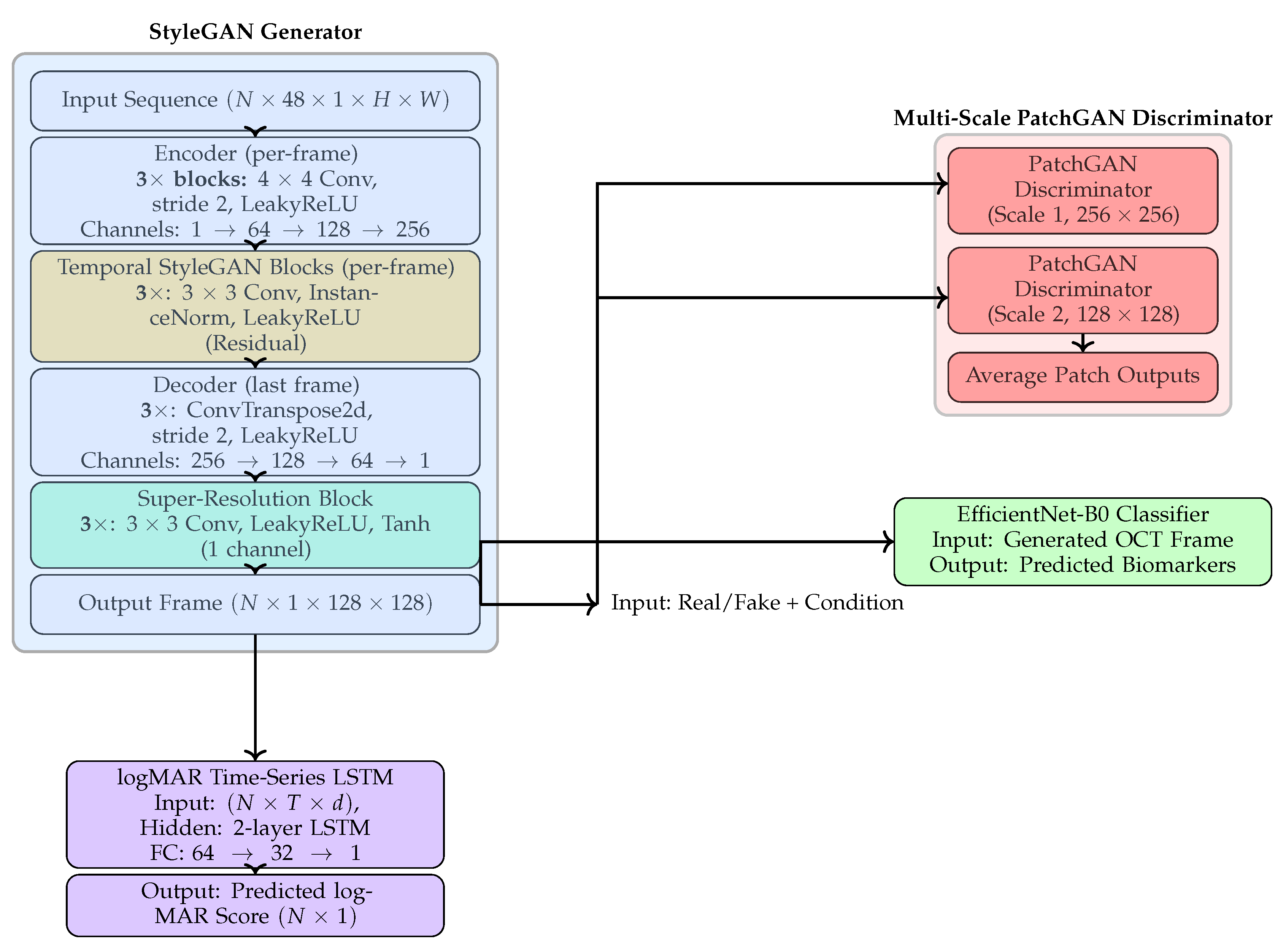
Figure 2.
Patient 232 class encoding: Winner (), Stabilizer (), Loser (). Prediction crosses match class color.
Figure 2.
Patient 232 class encoding: Winner (), Stabilizer (), Loser (). Prediction crosses match class color.
Figure 3.
Patient 234 logMAR trajectories using the same colorblind-safe classes: Winner, Stabilizer, Loser. Prediction crosses use matching class colors.
Figure 3.
Patient 234 logMAR trajectories using the same colorblind-safe classes: Winner, Stabilizer, Loser. Prediction crosses use matching class colors.
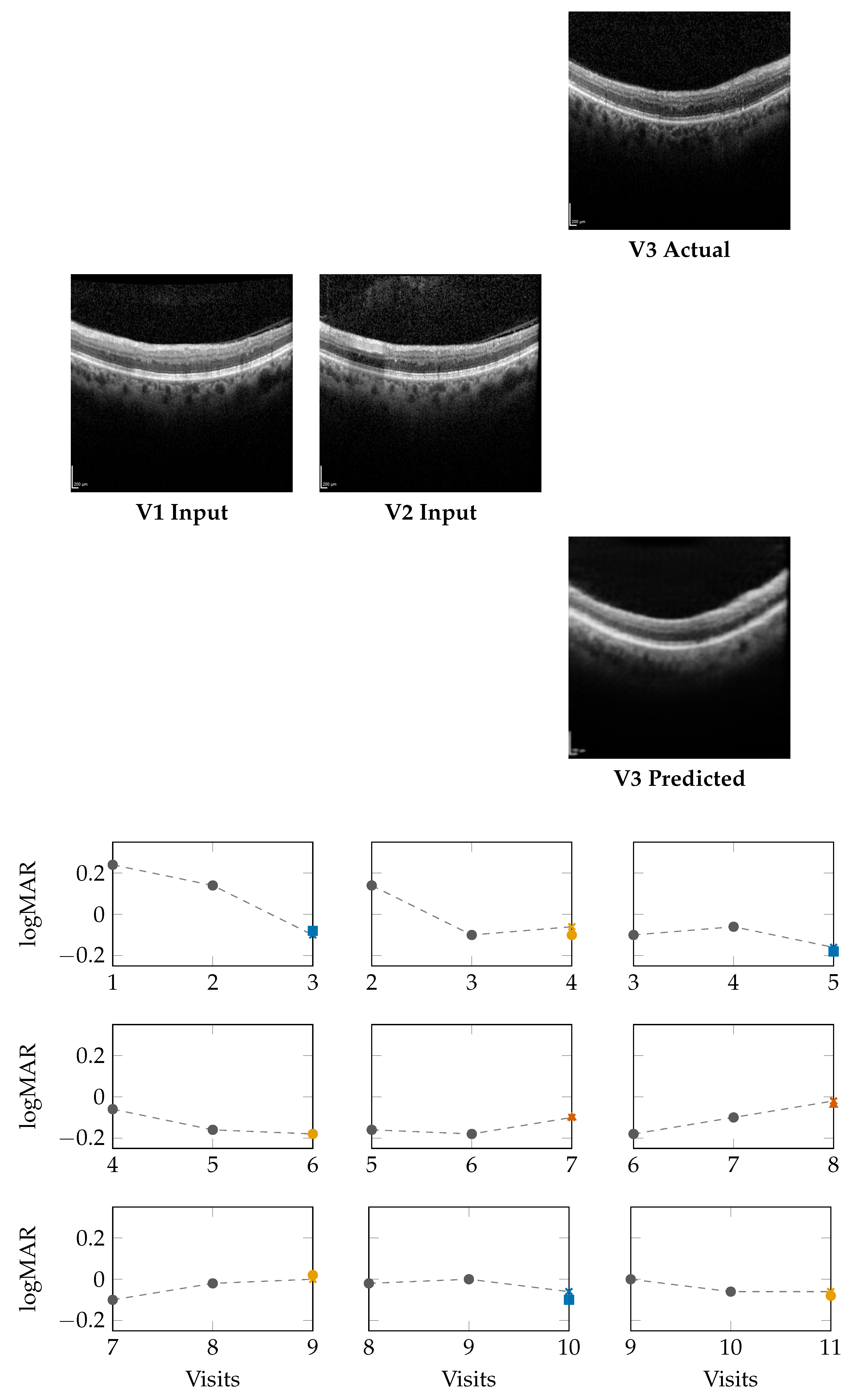
Figure 4.
Overall confusion matrix across the full test set (20 patients). Performance metrics are provided in Table 4.
Figure 4.
Overall confusion matrix across the full test set (20 patients). Performance metrics are provided in Table 4.
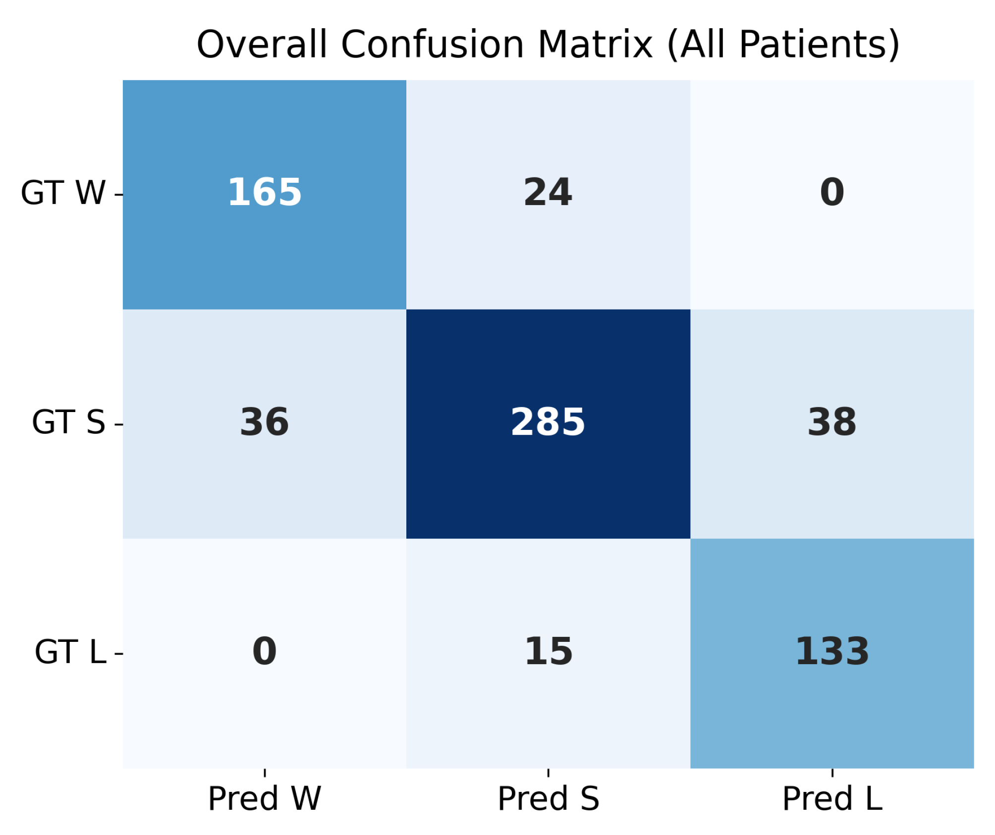
Figure 5.
Individual confusion matrices for the four patients arranged in a 2×2 layout, computed using the classification threshold . Performance metrics for each patient are reported in Table 4.
Figure 5.
Individual confusion matrices for the four patients arranged in a 2×2 layout, computed using the classification threshold . Performance metrics for each patient are reported in Table 4.
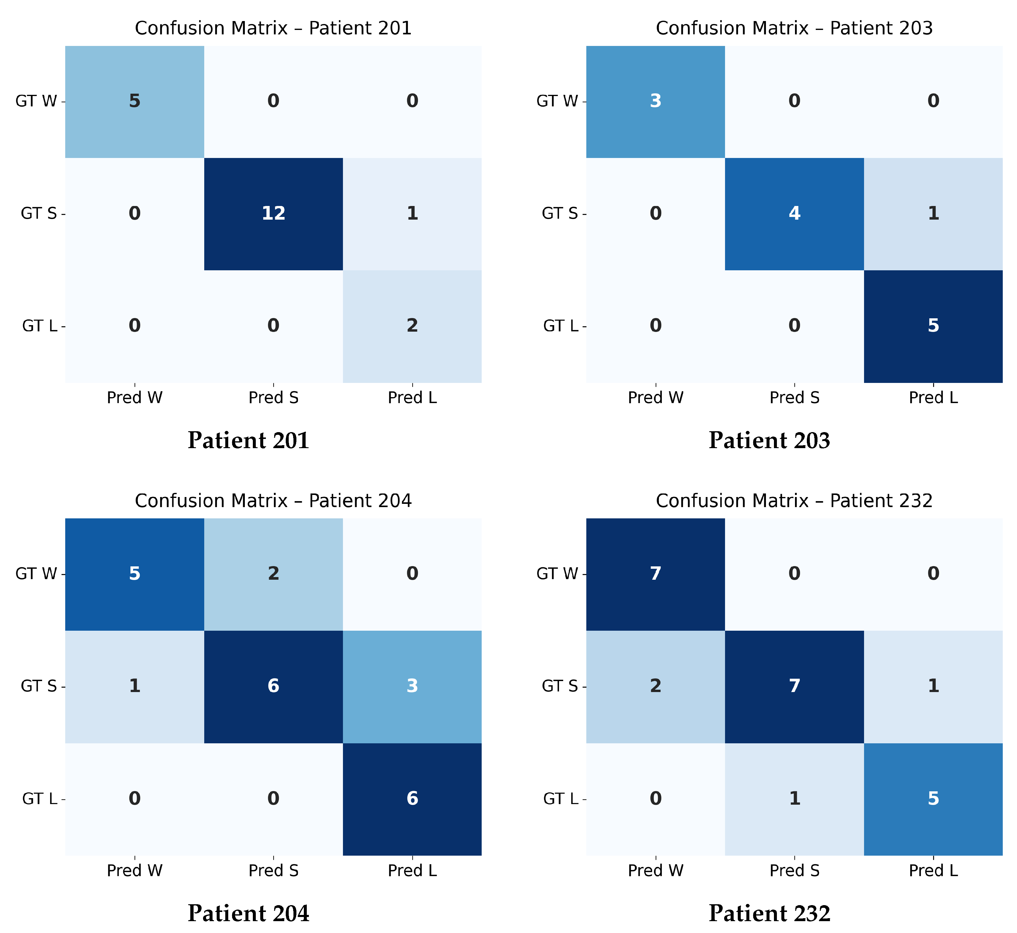
Table 2.
Performance comparison across model configurations using SSIM, PSNR, and FID. MAE and MSE apply only to the multimodal models (IDs 13–14), which jointly predict OCT frames and logMAR scores. Model ID-13 achieves MAE=0.078 and MSE=0.0066, while Model ID-14 achieves MAE=0.052 and MSE=0.0058.
Table 2.
Performance comparison across model configurations using SSIM, PSNR, and FID. MAE and MSE apply only to the multimodal models (IDs 13–14), which jointly predict OCT frames and logMAR scores. Model ID-13 achieves MAE=0.078 and MSE=0.0066, while Model ID-14 achieves MAE=0.052 and MSE=0.0058.
| ID | Input | Output | SSIM | PSNR | FID |
|---|---|---|---|---|---|
| 1 | v1, v2 | v3 | 0.5432 ± 0.012 | 21.3 ± 1.7 | 101.3 |
| 2 | v1, v2 | v3 | 0.7654 ± 0.009 | 27.8 ± 1.2 | 55.6 |
| 3 | v1, v2 | v3 | 0.7938 ± 0.010 | 29.3 ± 1.1 | 47.2 |
| 4 | v1, v2, v3 | v4 | 0.8232 ± 0.011 | 30.1 ± 1.0 | 38.8 |
| 5 | v1, v2, v3 | v4 | 0.8411 ± 0.010 | 31.3 ± 1.0 | 33.5 |
| 6 | v1, v2, v3, v4 | v5 | 0.8611 ± 0.009 | 32.8 ± 1.1 | 27.9 |
| 7 | v2, v3, v4, v5 | v6 | 0.8612 ± 0.010 | 32.9 ± 1.2 | 27.6 |
| 8 | v3, v4, v5 | v6 | 0.8727 ± 0.009 | 33.0 ± 1.1 | 25.8 |
| 9 | v4, v5, v6 | v7 | 0.8841 ± 0.008 | 33.5 ± 1.1 | 23.9 |
| 10 | v5, v6, v7 | v8 | 0.8732 ± 0.009 | 33.8 ± 1.0 | 24.7 |
| 11 | v6, v7, v8 | v9 | 0.8797 ± 0.008 | 34.1 ± 1.0 | 24.1 |
| 12 | v7, v8, v9 | v10 | 0.8864 ± 0.009 | 35.1 ± 1.0 | 22.8 |
| 13 | v1–v9 (2 pair) | v3–v10 | 0.8992 ± 0.007 | 36.2 ± 1.0 | 13.8 |
| 14 | v1–v9 (3 pair) | v3–v10 | 0.9264 ± 0.006 | 38.1 ± 0.9 | 11.9 |
Table 3.
Winner–Stabilizer–Loser counts for each Patient at different thresholds for GT and Predicted logMAR.
Table 3.
Winner–Stabilizer–Loser counts for each Patient at different thresholds for GT and Predicted logMAR.
| Patient | Class | 0.01 | 0.02 | 0.03 | 0.04 | 0.05 | 0.06 | 0.07 | 0.08 | 0.09 | 0.10 |
|---|---|---|---|---|---|---|---|---|---|---|---|
| Ground Truth (GT) | |||||||||||
| 201 | Winner | 5 | 6 | 7 | 8 | 8 | 8 | 8 | 8 | 8 | 8 |
| 201 | Stabilizer | 10 | 11 | 12 | 12 | 12 | 12 | 12 | 12 | 12 | 12 |
| 201 | Loser | 5 | 3 | 1 | 0 | 0 | 0 | 0 | 0 | 0 | 0 |
| 203 | Winner | 3 | 4 | 5 | 6 | 6 | 6 | 6 | 7 | 7 | 7 |
| 203 | Stabilizer | 9 | 10 | 11 | 12 | 12 | 12 | 12 | 12 | 12 | 12 |
| 203 | Loser | 4 | 3 | 2 | 1 | 1 | 1 | 1 | 1 | 1 | 1 |
| 232 | Winner | 2 | 2 | 3 | 3 | 2 | 1 | 1 | 1 | 1 | 1 |
| 232 | Stabilizer | 8 | 10 | 14 | 18 | 21 | 22 | 22 | 23 | 23 | 23 |
| 232 | Loser | 13 | 11 | 6 | 2 | 0 | 0 | 0 | 0 | 0 | 0 |
| 234 | Winner | 3 | 3 | 4 | 5 | 5 | 6 | 6 | 6 | 6 | 6 |
| 234 | Stabilizer | 8 | 9 | 10 | 11 | 11 | 12 | 12 | 12 | 12 | 12 |
| 234 | Loser | 6 | 5 | 4 | 2 | 1 | 0 | 0 | 0 | 0 | 0 |
| Predicted (Pred) | |||||||||||
| 201 | Winner | 6 | 7 | 7 | 8 | 8 | 8 | 8 | 8 | 8 | 8 |
| 201 | Stabilizer | 9 | 10 | 11 | 11 | 12 | 12 | 12 | 12 | 12 | 12 |
| 201 | Loser | 5 | 4 | 2 | 1 | 0 | 0 | 0 | 0 | 0 | 0 |
| 203 | Winner | 3 | 4 | 5 | 5 | 6 | 6 | 6 | 6 | 6 | 6 |
| 203 | Stabilizer | 9 | 10 | 11 | 12 | 12 | 12 | 12 | 12 | 12 | 12 |
| 203 | Loser | 4 | 3 | 2 | 1 | 1 | 1 | 1 | 1 | 1 | 1 |
| 232 | Winner | 3 | 3 | 3 | 3 | 2 | 1 | 1 | 1 | 1 | 1 |
| 232 | Stabilizer | 8 | 9 | 13 | 17 | 20 | 21 | 21 | 22 | 22 | 22 |
| 232 | Loser | 12 | 10 | 6 | 2 | 0 | 0 | 0 | 0 | 0 | 0 |
| 234 | Winner | 3 | 3 | 4 | 5 | 5 | 6 | 6 | 6 | 6 | 6 |
| 234 | Stabilizer | 8 | 9 | 10 | 11 | 11 | 12 | 12 | 12 | 12 | 12 |
| 234 | Loser | 6 | 5 | 4 | 2 | 1 | 0 | 0 | 0 | 0 | 0 |
Table 4.
Overall test-set (20 patients) and per-patient performance metrics using macro, micro, and weighted averaging across the three classes—Winner (W), Stabilizer (S), and Loser (L)—computed using the threshold .
Table 4.
Overall test-set (20 patients) and per-patient performance metrics using macro, micro, and weighted averaging across the three classes—Winner (W), Stabilizer (S), and Loser (L)—computed using the threshold .
| Patient | Prec (Ma) | Rec (Ma) | F1 (Ma) | Prec (Mi) | Rec (Mi) | F1 (Mi) | Prec (Wt) | Rec (Wt) | F1 (Wt) |
|---|---|---|---|---|---|---|---|---|---|
| Overall | 0.8261 | 0.8552 | 0.8382 | 0.8376 | 0.8376 | 0.8376 | 0.8420 | 0.8376 | 0.8376 |
| 201 | 0.8889 | 0.9744 | 0.9200 | 0.9500 | 0.9500 | 0.9500 | 0.9667 | 0.9500 | 0.9540 |
| 203 | 0.9444 | 0.9333 | 0.9327 | 0.9231 | 0.9231 | 0.9231 | 0.9359 | 0.9231 | 0.9223 |
| 204 | 0.7500 | 0.7714 | 0.7453 | 0.7391 | 0.7391 | 0.7391 | 0.7536 | 0.7391 | 0.7327 |
| 232 | 0.8287 | 0.8444 | 0.8287 | 0.8261 | 0.8261 | 0.8261 | 0.8345 | 0.8261 | 0.8219 |
Table 5.
Per-class biomarker classification performance (precision, recall, F1) for EfficientNet-B0 on OLIVES. Macro-F1 = 0.81.
Table 5.
Per-class biomarker classification performance (precision, recall, F1) for EfficientNet-B0 on OLIVES. Macro-F1 = 0.81.
| Biomarker | Precision | Recall | F1 Score |
|---|---|---|---|
| Atrophy/thinning of retinal layers | 0.82 | 0.79 | 0.80 |
| Disruption of ellipsoid zone (EZ) | 0.83 | 0.84 | 0.83 |
| Disorganization of retinal inner layers (DRIL) | 0.81 | 0.75 | 0.78 |
| Intraretinal hemorrhages (IR) | 0.70 | 0.74 | 0.72 |
| Intraretinal hyperreflective foci (IRHRF) | 0.76 | 0.80 | 0.78 |
| Partially attached vitreous face (PAVF) | 0.82 | 0.81 | 0.81 |
| Fully attached vitreous face (FAVF) | 0.85 | 0.83 | 0.84 |
| Preretinal tissue/hemorrhage | 0.77 | 0.79 | 0.78 |
| Vitreous debris (VD) | 0.80 | 0.78 | 0.79 |
| Vitreomacular traction (VMT) | 0.74 | 0.76 | 0.75 |
| Diffuse retinal thickening/macular edema (DRT/ME) | 0.86 | 0.85 | 0.85 |
| Intraretinal fluid (IRF) | 0.90 | 0.87 | 0.89 |
| Subretinal fluid (SRF) | 0.91 | 0.88 | 0.89 |
| RPE disruption | 0.83 | 0.82 | 0.83 |
| Serous PED | 0.76 | 0.78 | 0.77 |
| Subretinal hyperreflective material (SHRM) | 0.84 | 0.85 | 0.84 |
Disclaimer/Publisher’s Note: The statements, opinions and data contained in all publications are solely those of the individual author(s) and contributor(s) and not of MDPI and/or the editor(s). MDPI and/or the editor(s) disclaim responsibility for any injury to people or property resulting from any ideas, methods, instructions or products referred to in the content. |
© 2025 by the authors. Licensee MDPI, Basel, Switzerland. This article is an open access article distributed under the terms and conditions of the Creative Commons Attribution (CC BY) license (http://creativecommons.org/licenses/by/4.0/).
Copyright: This open access article is published under a Creative Commons CC BY 4.0 license, which permit the free download, distribution, and reuse, provided that the author and preprint are cited in any reuse.


