
Submitted:
26 November 2025
Posted:
02 December 2025
You are already at the latest version
Abstract
In this study, we present a systematic evaluation of Synolitic Graph Neural Networks (SGNNs), a novel framework that transforms high-dimensional tabular data into sample-specific graphs using ensembles of low-dimensional pairwise classifiers. We demonstrate that augmenting these graphs with topology-aware node descriptors (such as degree, strength, closeness, and betweenness centrality) and applying graph sparsification techniques, either via minimum spanning connectivity or fixed-probability edge retention, can significantly improve classification performance. We evaluate both convolution-based (GCN) and attention-based graph neural networks (GATv2) across two training regimes: a foundation model setting where multiple datasets are concatenated, and dataset-specific training. Results show that attention-based models generally exhibit superior performance across classification tasksвАФin the foundation regime, dense (non-sparsified) graphs with node features yield 92.83 ROC-AUC for GATv2 and 92.34 for GCN (vs. 90.80 for XGBoost), and in the dataset-specific regime, GATv2 with minimal connectivity and node features reaches 88.96 ROC-AUC (vs. 86.84 for XGBoost). A leave-one-dataset-out evaluation further indicates out-of-domain transfer to previously unseen datasets (mean ROC-AUC: 0.78 with node features; 0.71 with maximum-threshold sparsification; 0.70 without features). Importantly, we demonstrate that the SGNN framework is capable of overcoming the curse of dimensionality, outperforming traditional machine learning models such as XGBoost in scenarios where the number of features exceeds the number of training samplesвАФmaintaining ROC-AUC above 80\% with only 5\% of the training data, while XGBoost drops to 60\%. Furthermore, SGNNs exhibit robustness to feature redundancy and correlation, with duplicating all features and adding noise producing only minor deviations, reducing the need for manual feature engineering or dimensionality reduction. Across all settings, SGNNs enhanced with node features consistently outperform XGBoost baselines, underscoring the effectiveness of integrating graph-based structural representations, topology-aware augmentation, and controlled sparsification in classification tasks.
Keywords:
synolitic topology
; graph neural networks
; high-dimensional data
; tabular classification
1. Introduction
In recent years, artificial intelligence (AI) has experienced unprecedented growth, particularly in the domain of Large Language Models (LLMs)—transformer-based architectures trained on massive text corpora [1]. These models exhibit remarkable capabilities and represent a significant step toward general, even superhuman, AI. A prominent study by Epoch AI [2] recently made headlines by quantifying a looming challenge: by around 2028, the average dataset size used to train AI models is expected to reach the total estimated stock of all publicly available online text. In other words, AI may run out of new training data within the next few years [3]. In contrast, the situation in biology and physiology is qualitatively different. Access to diverse clinical, physiological, and cognitive datasets has expanded dramatically. Today, we can sequence the human genome with near-complete resolution [4], map the proteome and transcriptome, especially with focus on single-cell omics [5], monitor DNA methylation across millions of genomic loci [6], and collect high-resolution physiological and imaging data—including EEG, ECG, CT, MRI, fMRI, and MEG. Moreover, there is now widespread availability of structured and unstructured Electronic Health Records (EHRs) [7].
Despite substantial progress and increasing volume of data, translating complex, high-dimensional biomedical data into actionable clinical knowledge remains difficult. For many specific medical problems the amount of clean data available for machine learning remains very small. These datasets are heterogeneous and often longitudinal, spanning genomics, proteomics, physiological signals, medical imaging, and electronic health records (EHRs), and each modality raises distinct challenges for interpretable machine learning [8]. Traditional approaches suffer from the curse of dimensionality: as feature counts grow, the samples required to maintain generalizability increase exponentially, which is rarely feasible in healthcare due to high acquisition costs, ethical constraints, and limited patient cohorts, leading to overfitting and weak predictive performance [9]. Compounding this, many deep learning models lack interpretability and transparency, needed to achieve trust and to replace an expert opinion in clinical implementation [8]. Although recent advances thrive on images and text, they frequently fail to generalize to structured biomedical representations, such as patient graphs, brain connectomes, or molecular interaction networks, without substantial domain-specific preprocessing [10].
There are three primary requirements for AI algorithms designed to analyse clinical data:
- Robustness to heterogeneity. They must detect diverse and hidden patterns that may lead to the same clinical outcome, recognising that compensatory mechanisms can produce similar disease manifestations via different pathways;
- Data efficiency. They must be capable of learning from small sample sizes, given the scarcity and cost of clinical data;
- Interpretability. They must go beyond simple classification and offer insightful, explainable reasoning, and even better the test procedure to verify the conclusion, especially for tasks such as early diagnosis and risk stratification.
In this context, graph-based AI methods emerge as particularly promising. The human body itself is naturally organised as a multi-layered, interconnected system - a "network of networks" [11]. Organs interact within physiological systems, regulated by the brain, which is itself a complex network of neurons and astrocytes. At the molecular level, cellular processes such as growth, development, ageing, and disease progression (e.g., tumorigenesis) are governed by dynamic epigenetic and transcriptional regulatory networks, with growing recognition of the role of non-coding RNAs in shaping these interactions.
Thus, representing clinical and physiological data as graphs, mathematical structures that capture relationships between elements, aligns naturally with the biological architecture of the human body. By leveraging the topological and relational properties of such data, graph-based models offer a powerful framework for capturing complexity, enabling robust predictions, and uncovering mechanistic insights that are critical for advancing precision medicine [12].
One of the earliest approaches to transforming tabular biomedical data into graphs was proposed by Zanin and Boccaletti in the form of parenclitic networks [13]. Using linear regression, this method constructs sample-specific graphs by modeling expected pairwise feature relationships in control samples. Deviations from these relationships in case samples define edges in the graph. Topological metrics of these graphs can then be used as features in downstream classifiers, embedding high-dimensional data into a lower-dimensional and interpretable space. This approach has been successfully applied to gene expression, metabolomics, and epigenetic datasets [14].
Despite their utility, parenclitic networks have limitations, including reliance on linear assumptions, thresholding sensitivity, and poor scalability to multimodal or large-scale data. To address these issues, later work introduced enhancements such as using two-dimensional kernel density estimation (2DKDE) instead of linear regression [15], and edge weighting schemes that reflect deviation magnitudes. These improvements led to more accurate class separation and greater biological interpretability.
Building upon these developments, Synolitic Graph Neural Networks (SGNNs) [10] offer a more scalable and generalizable alternative. SGNNs construct graphs using an ensemble of low-dimensional classifiers trained on all pairwise feature combinations. These graphs are class-specific and do not require any domain-specific knowledge or anatomical priors. Unlike traditional Graph Neural Networks (GNN) models tailored to specific domains (e.g., BrainGNN for fMRI), SGNNs generalize across data types and support continuous and categorical variables. SGNNs have shown promise in prior applications such as ageing trajectory analysis [16], prognosis in COVID-19 patients [17,18], and epigenetic profiling in cancer and Down syndrome [16]. These studies demonstrate the potential of SGNN-derived graph representations to uncover biologically meaningful patterns.
However, existing work has primarily focused on the generation of graph embeddings. To date, it remains unclear how different downstream GNN architectures can exploit these embeddings to perform classification effectively. This work presents the first systematic Synolitic Graph Neural Networks (SGNNs) evaluation for high-dimensional tabular classification. We transform high-dimensional, heterogeneous datasets into sample-specific graphs via ensembles of pairwise low-dimensional classifiers and enrich them with topology-aware node descriptors (degree, strength, closeness, betweenness) and multiple sparsification strategies (top-p edges, minimum-connected). We benchmark two representative GNNs—GCN (convolution-based [19]) and GATv2 (attention-based [20])—in two regimes: (i) a foundation setting on a concatenation of 15 UCI datasets (selected via the Mirkes et al. taxonomy [21]) to probe cross-task generalization, and (ii) dataset-specific training to assess within-domain performance.
We show that across both regimes, inducing graph structure and augmenting node features combined with edge-based sparsification consistently improves predictive performance over strong tabular baselines (XGBoost), is robust to feature redundancy, showing promising out-of-domain generalization across datasets. Together, these results position SGNNs as a practical route for learning from high-dimensional, heterogeneous biomedical data.
2. Materials and Methods
2.1. Datasets
We evaluate publicly available binary classification tabular datasets from the UCI Machine Learning Repository. We selected these datasets based on criteria proposed by Mirkes et al. [21], ensuring consistency and relevance to biomedical-like settings. Selection criteria include:
- Binary class labels;
- No missing values;
- All features are numerical or binary;
- The number of samples exceeds the number of features.
These datasets provide a varied testbed to assess model generalizability across domains with differing feature dimensions, sample sizes, and class distributions. In this report, we restricted our selection to 15 datasets illustrated in Figure 1, for which the construction of sample-specific graphs is computationally feasible within acceptable time constraints, providing a balanced trade-off between dataset diversity and experimental practicality.
To evaluate classification procedure, we report the Area Under the Receiver Operating Characteristic Curve (ROC-AUC), a standard metric that reflects the trade-off between the true positive rate (sensitivity) and the false positive rate across classification thresholds.
2.2. Models
2.2.1. Pipeline Architecture
SGNNs constitute a general-purpose framework for converting high-dimensional data into graph representations [10]. The method constructs sample-specific graphs by training an ensemble of pairwise classifiers using class labels. All nodes of our graph are features of dataset. A binary classifier, typically a Support Vector Machine (SVM) or a two-dimensional kernel density estimator (2DKDE), learns the decision boundary between classes in its respective 2D projection for each unique feature pair. The score of each classifier is used to define edge weights between corresponding feature nodes in the graph, where nodes represent features and edges encode class-separation strength.
This transformation yields one graph per sample, which is subsequently processed by a GNN that operates on graph structure and edge weights to produce a classification for each input sample. An overview of this process is presented in Figure 2, which illustrates how SGNNs can accommodate diverse data modalities, including numerical features, categorical variables, imaging, and electronic health records.
In this report, we evaluate the effectiveness of two state-of-the-art GNN architectures as downstream classifiers operating on SGNN-derived graphs:
The parameters for GNNs experiments are presented in Table 1. To evaluate the proposed SGNN methodology, we designed a structured experimental pipeline. This pipeline includes distinct stages encompassing graph construction, model training, and performance benchmarking. Each stage was tailored to systematically assess the effectiveness and generalizability of the approach across diverse biomedical datasets. The experimental procedure consists of the following stages:
- (1)
- SGNN Graph Construction. We generate sample-specific graphs from selected tabular datasets using the SGNN methodology, which relies on ensembles of pairwise classifiers trained with class labels for each dataset and produces a unique graph structure for every data point [10].
- (2)
- GNN Training. We train two graph neural networks — GCN and GATv2 — on the resulting graphs to perform classification. For each model and each task, we use training parameters selected individually through hyperparameter optimization using the Optuna framework [22].
- (3)
- Training Strategies. We evaluate two training regimes: (i) training on the concatenation of all datasets as a form of task-agnostic pretraining or foundation model setting, and (ii) individual training on each dataset separately. Exploration of these settings allows us to examine generalization across datasets.
- (4)
- Comparison with Classical Models. We compare our graph-based approaches with a classical XGBoost classifier trained on the same datasets, to assess the relevance and added value of GNNs in this classification context.
2.2.2. Node Features
To enrich the initial graph representation, that is the full graph, we augment nodes with structural features that capture their topological properties within the network. Starting from the original scalar node feature, we construct a five-dimensional feature vector:
where:
- is the original scalar feature of node i;
- is the normalized node degree, i.e., the normalised number of edges connected to this node: , where N is the number of nodes;
- is the normalized node strength: , where and is an edge weight between nodes i and j;
- is the closeness centrality of node i, calculated as the reciprocal of the sum of the length of the shortest paths between the node and all other nodes in the graph;
- is the betweenness centrality of node i computed with edge weights.
This combination of features enables the model to consider both local node characteristics (degree, strength) and global structural importance (centrality measures) within the graph topology.
2.2.3. Graph Sparsification
To investigate the impact of edge density on prediction quality, we implement three graph sparsification strategies:
- (1)
- Threshold-based sparsification: Retains a fraction p of the most significant edges based on the criterion , where is the edge weight. This approach allows control over graph sparsity while preserving connections with the greatest deviation from the neutral value 0.5.
- (2)
- Minimum connected sparsification: Employs binary search to determine the maximum threshold such that the graph remains connected. The method finds the minimal edge set that ensures graph connectivity, thereby optimizing the trade-off between sparsity and structural integrity.
- (3)
- No sparsification: Baseline configuration that preserves the original graph structure.
These sparsification methods enable investigation of the compromise between computational efficiency and preservation of important structural information in molecular graphs.
3. Results
3.1. Foundation Model Task
To assess the generalizability and scalability of the SGNN pipeline, we conducted experiments in the foundation setting: we merge all selected UCI datasets into a single, unified classification problem to test whether SGNN-derived graphs capture patterns that generalize across heterogeneous domains. Table 2 shows that node features and sparsification improve ROC-AUC in the foundation setting, especially with node features, outperforming the XGBoost baseline (90.80). The best overall result is shown by GATv2 without sparsification and using node features (92.83), with its sparsified with version close behind (92.39). Without node features, the strongest configuration is GATv2 on the slightly sparsified (p=0.2) graph (91.01). From an architectural standpoint, these results indicate that once node-level descriptors are available, dense connectivity is optimal—both GATv2 and GCN peak with no sparsification (92.83 and 92.34, respectively), while pruning generally reduces performance. In the absence of node features, light sparsification (p=0.2) can yield a small gain for attention-based GATv2, but aggressive sparsification and minimum-connected backbones do not help. Overall, node features drive the majority of gains, and attention benefits most from retaining dense message-passing pathways in the foundation setting.
3.2. Separate Datasets Task
To systematically evaluate the effectiveness of the proposed SGNN pipeline, we applied it to each dataset individually, with performance summarized as the macro-averaged ROC-AUC across all evaluated datasets. In the separate-datasets task, Table 3 shows that GATv2 consistently surpasses XGBoost (86.84 macro ROC-AUC) across sparsification strategies, with the best result at minimal connectivity sparsification with node features (88.96); the unpruned configuration with features also scores 88.35. GCN is generally weaker than GATv2 here; its peak is 87.77 with no sparsification and node features. Generally, enabling node features consistently boosts performance for both GNNs, outperforming the XGBoost baseline, while for attention-based GNNs without node features overly aggressive pruning or minimum-connectivity tends to underperform relative to moderate sparsification.
3.3. Visualization of Sparsification Strategies
Table 4 visually compares different sparsification strategies applied to sample-specific graphs: fully connected graphs, top 20% most significant edges, and minimum threshold graphs that preserve connectivity. The examples demonstrate how edge pruning impacts graph structure for both positive and negative class samples, with more aggressive sparsification yielding sparser yet still interpretable topologies.
3.4. Testing the Universality of the Pipeline
To evaluate the generalization capability of the SGNN pipeline, we adopted a leave-one-out evaluation strategy across multiple datasets. In this experimental design, the model was trained on Synolitic graphs constructed from all datasets except one, which was held out for testing. This procedure was repeated for each dataset, ensuring that every dataset served as an independent test domain. The SGNN architecture was kept fixed across all runs, using GATv2, which demonstrated the best overall performance in Section 3.2. To ensure consistency and isolate the effects of cross-dataset transfer, we employed its base configuration without additional hyperparameter tuning. This setup allowed us to assess how well the model can transfer knowledge learned from diverse high-dimensional datasets to previously unseen domains.
As shown in Table 5, the SGNN pipeline demonstrated consistent cross-domain generalization. The model trained on synolitic graphs only achieved a macro ROC-AUC of 70.34%, while sparsification at the maximum threshold slightly improved it to 71.07%. Notably, incorporating additional node features further enhanced transferability, yielding the best macro ROC-AUC of 78.39%. These results suggest that topology-aware node descriptors play a key role in capturing structural patterns that are shared across heterogeneous biomedical datasets, enabling the SGNN framework to generalize effectively to previously unseen domains.
3.5. Dealing with the Curse of Dimensionality
To evaluate the performance of the SGNN pipeline in high-dimensional, low-sample settings, we conducted a series of benchmark experiments across all 15 datasets, taking all the parameters as in Section 3.2 when we applied the pipeline to each dataset individually. To simulate increasingly data-scarce conditions, we further reduced the size of the training set in systematic increments, down to 5% of the original training size. We then compared the classification performance of SGNNs to that of a standard ensemble-based machine learning model, XGBoost, which is widely recognized for its robustness and performance in structured data tasks. As shown in Figure 3, XGBoost exhibited a marked degradation in performance as the training data size decreased, with ROC-AUC scores dropping below 60% when less than 20% of the training set was used. In contrast, the SGNN pipeline maintained strong and stable performance across all data regimes, with ROC-AUC scores consistently above 80% even under the most constrained conditions.
These findings highlight several key advantages of the SGNN approach. First, its reliance on low-dimensional classifiers enables effective training even when the number of samples is small relative to the number of features—directly addressing the "curse of dimensionality." Second, the use of graph-based representations allows the model to capture complex, higher-order relationships among features that are otherwise difficult to encode with traditional methods. Third, the ensemble graph construction provides robustness against sampling variability and enables generalisation across small, heterogeneous datasets.
Taken together, these results demonstrate that SGNNs offer a powerful and scalable alternative to conventional machine learning models in diverse applications where high-dimensional data and limited sample sizes are the norm. The ability to retain high classification accuracy under such constraints makes SGNNs particularly well-suited for early-stage clinical research, rare disease modelling, and other settings where data availability is inherently limited.
3.6. Robustness to Correlated Features
A common question that arises in the context of our methodology is whether traditional preprocessing steps—such as scaling, normalisation, and feature selection—are still required. Indeed, transforming multimodal data into predictive classifiers typically involves a complex and often lengthy pipeline. While the proposed SGNN approach simplifies certain aspects by leveraging low-dimensional classifiers (LDCs) to extract topological structure from high-dimensional data, it does not entirely eliminate the need for data wrangling. Rather, these challenges are shifted to an earlier stage in the pipeline, prior to graph construction and learning. In particular, scaling and harmonisation of input modalities, as well as effective strategies for integrating multi-omics or multi-modal datasets, remain critical considerations.
It is also well-established that as the number of features increases, the number of samples required for reliable model training grows exponentially—an expression of the "curse of dimensionality" [23]. Constructing robust models in lower-dimensional subspaces can mitigate this, but it first requires the accurate identification of the relevant subspace. While this step may ultimately reduce the sample size needed for downstream tasks, determining such a subspace in a manner that generalises well still demands a substantial amount of data.
However, preliminary experiments with the SGNN pipeline suggest that explicit feature engineering or dimensionality reduction may not be necessary. To investigate this, we conducted an experiment in which we used pipeline from Section 3.2 and duplicated the entire set of features while introducing a 5% amount of Gaussian noise, effectively doubling the dimensionality of the data. The full SGNN pipeline was then applied to these modified datasets. As summarised in Table 6, the resulting ROC-AUC scores showed minimal deviation from the original results—and in some cases, even improved slightly. These findings indicate that SGNNs are robust to noise and high-dimensional input, and that the pipeline itself can implicitly identify relevant structures without additional preprocessing steps.
In summary, while traditional concerns about high dimensionality and data integration remain valid, the SGNN pipeline demonstrates an inherent resilience to these issues. Its ability to maintain performance without the need for extensive feature engineering represents a significant advantage in the analysis of complex high-dimensional datasets.
4. Discussion
In this study, we systematically evaluated Synolitic Graph Neural Networks (SGNNs) as a way to convert high-dimensional data into sample-specific graphs by benchmarking downstream GNN classifiers under different sparsification regimes and topology-aware node features, focusing on the task of tabular classification, including biomedical applications. Our results demonstrate that augmenting SGNN-derived graphs with node-level topological features and carefully chosen sparsification consistently improves classification performance. The foundation regime achieved the strongest performance with dense (non-sparsified) graphs combined with node features, as shown by GATv2 (ROC-AUC = 92.83%) and GCN (ROC-AUC = 92.34%). In the per-dataset regime, GATv2 performed best with the minimal connectivity sparsification strategy and node features (88.96% ROC-AUC). Across both regimes, GNNs with node features surpassed the XGBoost baseline (90.80% / 86.84% ROC-AUC), highlighting the effectiveness of leveraging SGNN-induced structure and its topology-aware node descriptors for tabular classification.
Beyond these regimes, leave-one-dataset-out evaluation indicates out-of-domain transfer to previously unseen datasets. SGNNs also remain effective in small-sample settings—maintaining ROC-AUC above 80% with only 5% of the training data while XGBoost drops to 60%—and are robust to feature redundancy and missingness: duplicating features with added noise yields only minor deviations, and absent features simply remove the corresponding nodes/edges without destabilizing learning. Ablations confirm that node-level topology is the primary driver of gains, whereas sparsification is beneficial only insofar as it avoids overly aggressive pruning that would hinder message passing. These findings underscore the promise of SGNNs as a principled approach for representing diverse data modalities as graphs and enhancing the performance of modern GNN architectures.
This study presents a systematic evaluation of Synolitic Graph Neural Networks (SGNNs), a novel and versatile methodology for transforming high-dimensional data of diverse origin into graph-based representations. The innovation lies in constructing Synolitic Graphs by applying low-dimensional classifiers (LDCs) trained solely on class labels, and subsequently analysing these graphs using Graph Neural Networks (GNNs). While GNNs are currently the main analytical tool within this framework, the underlying pipeline remains methodologically flexible and can incorporate a wide range of graph-based classification techniques, including statistical approaches such as multivariate logistic regression based on graph topology. The conceptual foundation of Synolitic Networks is rooted in earlier work on Parenclitic Networks and has been successfully validated across several domains, including DNA methylation analysis, early cancer detection through proteomic profiles, fMRI-based brain state classification, and the study of epigenetic alterations in Down syndrome.
One of the central findings from our evaluation is the adaptability and extensibility of the Synolitic framework. The pipeline allows different machine learning algorithms to be used for pairwise feature classification, supports multiple graph construction strategies (including standard and hypergraph representations), and can integrate a variety of AI techniques for final classification. This modularity ensures that each component—from LDCs to graph classifiers—can be readily updated or replaced as new architectures emerge in the rapidly evolving field of AI. Beyond its immediate applications in high-dimensional data analysis, the broader conceptual utility of Synolitic Networks is also evident. For instance, they offer a promising paradigm for modular and compositional AI, including applications to the architecture of Large Language Models, where smaller subnetworks operate in reduced feature spaces and communicate across a structured graph of interactions.
A key strength of the SGNN approach lies in its ability to mitigate the curse of dimensionality, a common challenge in clinical and omics data where the number of features often far exceeds the number of samples. We initially observed this advantage in our earlier study published in [24], and subsequently verified it here across 15 benchmark datasets. When evaluating classification performance on progressively smaller training sets, we found that conventional machine learning models such as XGBoost suffered marked reductions in accuracy as the sample size decreased. In contrast, SGNNs maintained robust performance, achieving ROC-AUC scores above 80%, even when trained on as little as 5% of the data—whereas XGBoost performance dropped to approximately 60%. These results underscore SGNNs’ superior generalisation ability in high-dimensional, low-sample regimes.
Finally, SGNNs reduce the need for heavy feature engineering and handle missing data gracefully. Because LDCs capture nonlinear, heterogeneous relations directly in low-dimensional subspaces and aggregate them into graph topology, salient patterns are encoded without prior feature selection or dimensionality reduction. Missing features simply remove the corresponding nodes/edges for a sample’s graph, leaving the remaining structure intact and enabling stable inference under incomplete observations. We will further investigate and validate this behavior across additional datasets and scenarios as part of the ongoing project. Taken together, the design choices—topology-aware construction, modularity, and robustness—complement the quantitative gains reported above and support SGNNs as a practical, extensible route to learning from heterogeneous, high-dimensional data of diverse origin.
Author Contributions
Conceptualization, A.Z, E.M.M, T.T; methodology,I.S.,A.S,A.L., R.N., A.Z.; validation, I.S.,A.S,A.L.,R.N.; writing—original draft preparation, All authors; All authors have read and agreed to the published version of the manuscript.
Funding
This work was supported by the Ministry of Economic Development of the Russian Federation (grant No 139-15-2025-004 dated 17 April 2025, agreement identifier 000000C313925P3X0002).
Data Availability Statement
All data used here are publicly available. The code is available at https://github.com/AlexeyZaikin/Synolitic-Graph-Neural-Networks.
Conflicts of Interest
All authors declare no conflicts of interest.
References
- Minaee, S.; Mikolov, T.; Nikzad, N.; Chenaghlu, M.; Socher, R.; Amatriain, X.; Gao, J. A: Language Models, 2025; arXiv:cs.CL/2402.06196].
- Villalobos, P.; Ho, A.; Sevilla, J.; Besiroglu, T.; Heim, L.; Hobbhahn, M. data. In Proceedings of the Proceedings of the 41st International Conference on Machine Learning; Salakhutdinov, R.; Kolter, Z.; Heller, K.; Weller, A.; Oliver, N.; Scarlett, J.; Berkenkamp, F., Eds. PMLR, 21–27 Jul 2024, Vol. 235, Proceedings of Machine Learning Research, pp.
- Jones, N. The AI revolution is running out of data. What can researchers do? Nature 2024, 636, 290–292. [Google Scholar] [CrossRef] [PubMed]
- Nurk, S.; Koren, S.; Rhie, A.; Rautiainen, M.; Bzikadze, A.V.; Mikheenko, A.; Vollger, M.R.; Altemose, N.; Uralsky, L.; Gershman, A.; et al. The complete sequence of a human genome. Science 2022, 376, 44–53. [Google Scholar] [CrossRef] [PubMed]
- A focus on single-cell omics. Nat Rev Genet 2023, 24, 485. [CrossRef] [PubMed]
- Schübeler, D. Function and information content of DNA methylation. Nature 2015, 517, 321–326. [Google Scholar] [CrossRef] [PubMed]
- Wang, L.; Yin, Y.; Glampson, B.; Peach, R.; Barahona, M.; Delaney, B.C.; Mayer, E.K. Transformer-based deep learning model for the diagnosis of suspected lung cancer in primary care based on electronic health record data. EBioMedicine 2024, 110. [Google Scholar] [CrossRef] [PubMed]
- Rahnenführer, J.; De Bin, R.; Benner, A.; Ambrogi, F.; Lusa, L.; Boulesteix, A.L.; Migliavacca, E.; Binder, H.; Michiels, S.; Sauerbrei, W.; et al. Statistical analysis of high-dimensional biomedical data: a gentle introduction to analytical goals, common approaches and challenges. BMC Medicine 2023, 21, 182. [Google Scholar] [CrossRef] [PubMed]
- Berisha, V.; Krantsevich, C.; Hahn, P.R.; Hahn, S.; Dasarathy, G.; Turaga, P.; Liss, J. Digital medicine and the curse of dimensionality. npj Digital Medicine 2021, 4, 153. [Google Scholar] [CrossRef] [PubMed]
- Krivonosov, M.; Nazarenko, T.; Ushakov, V.; Vlasenko, D.; Zakharov, D.; Chen, S.; Blyus, O.; Zaikin, A. Analysis of Multidimensional Clinical and Physiological Data with Synolitical Graph Neural Networks. Technologies 2025, 13. [Google Scholar] [CrossRef]
- Whitwell, H.J.; Bacalini, M.G.; Blyuss, O.; Chen, S.; Garagnani, P.; Gordleeva, S.Y.; Jalan, S.; Ivanchenko, M.; Kanakov, O.; Kustikova, V.; et al. The Human Body as a Super Network: Digital Methods to Analyze the Propagation of Aging. Frontiers in Aging Neuroscience, 2020. [Google Scholar] [CrossRef]
- Wu, Z.; Pan, S.; Chen, F.; Long, G.; Zhang, C.; Yu, P.S. A Comprehensive Survey on Graph Neural Networks. IEEE Transactions on Neural Networks and Learning Systems 2021, 32, 4–24. [Google Scholar] [CrossRef] [PubMed]
- Zanin, M.; Alcazar, J.M.; Carbajosa, J.V.; Paez, M.G.; Papo, D.; Sousa, P.; Menasalvas, E.; Boccaletti, S. Parenclitic networks: uncovering new functions in biological data. Scientific Reports 2014, 4, 5112. [Google Scholar] [CrossRef] [PubMed]
- Zanin, M.; Papo, D.; Sousa, P.; Menasalvas, E.; Nicchi, A.; Kubik, E.; Boccaletti, S. Combining complex networks and data mining: Why and how. Physics Reports 2016, 635, 1–44. [Google Scholar] [CrossRef]
- Whitwell, H.J.; Blyuss, O.; Menon, U.; Timms, J.F.; Zaikin, A. Parenclitic networks for predicting ovarian cancer. Oncotarget 2018, 9, 22717–22726. [Google Scholar] [CrossRef] [PubMed]
- Krivonosov, M.; Nazarenko, T.; Bacalini, M.G.; Vedunova, M.; Franceschi, C.; Zaikin, A.; Ivanchenko, M. Age-related trajectories of DNA methylation network markers: A parenclitic network approach to a family-based cohort of patients with Down Syndrome. Chaos, Solitons and Fractals 2022, 165, 112863. [Google Scholar] [CrossRef]
- Demichev, V.; Tober-Lau, P.; Lemke, O.; Nazarenko, T.; Thibeault, C.; Whitwell, H.; Röhl, A.; Freiwald, A.; Szyrwiel, L.; Ludwig, D.; et al. A time-resolved proteomic and prognostic map of COVID-19. Cell Systems 2021, 12, 780–794.e7. [Google Scholar] [CrossRef] [PubMed]
- Demichev, V.; Tober-Lau, P.; Nazarenko, T.; Lemke, O.; Kaur Aulakh, S.; Whitwell, H.J.; Röhl, A.; Freiwald, A.; Mittermaier, M.; Szyrwiel, L.; et al. A proteomic survival predictor for COVID-19 patients in intensive care. PLOS Digit Health 2022, 1, e0000007. [Google Scholar] [CrossRef] [PubMed]
- Kipf, T.N.; Welling, M. 2017; arXiv:cs.LG/1609.02907].
- Brody, S.; Alon, U.; Yahav, E. How Attentive are Graph Attention Networks? 2022; arXiv:cs.LG/2105.14491]. [Google Scholar]
- Mirkes, E.M.; Allohibi, J.; Gorban, A. Fractional Norms and Quasinorms Do Not Help to Overcome the Curse of Dimensionality. Entropy 2020, 22. [Google Scholar] [CrossRef] [PubMed]
- Akiba, T.; Sano, S.; Yanase, T.; Ohta, T.; Koyama, M. 2019; arXiv:cs.LG/1907.10902].
- Altman, N.; Krzywinski, M. The curse (s) of dimensionality. Nat Methods 2018, 15, 399–400. [Google Scholar] [CrossRef] [PubMed]
- Nazarenko, T.; Whitwell, H.J.; Blyuss, O.; Zaikin, A. Parenclitic and Synolytic Networks Revisited. Frontiers in Genetics, 2021. [Google Scholar] [CrossRef]
Figure 1.
Statistics of the 15 UCI tabular datasets used in this study, illustrating the diversity in feature dimensionality that underpins the evaluation of Synolitic Graph Neural Networks.
Figure 1.
Statistics of the 15 UCI tabular datasets used in this study, illustrating the diversity in feature dimensionality that underpins the evaluation of Synolitic Graph Neural Networks.
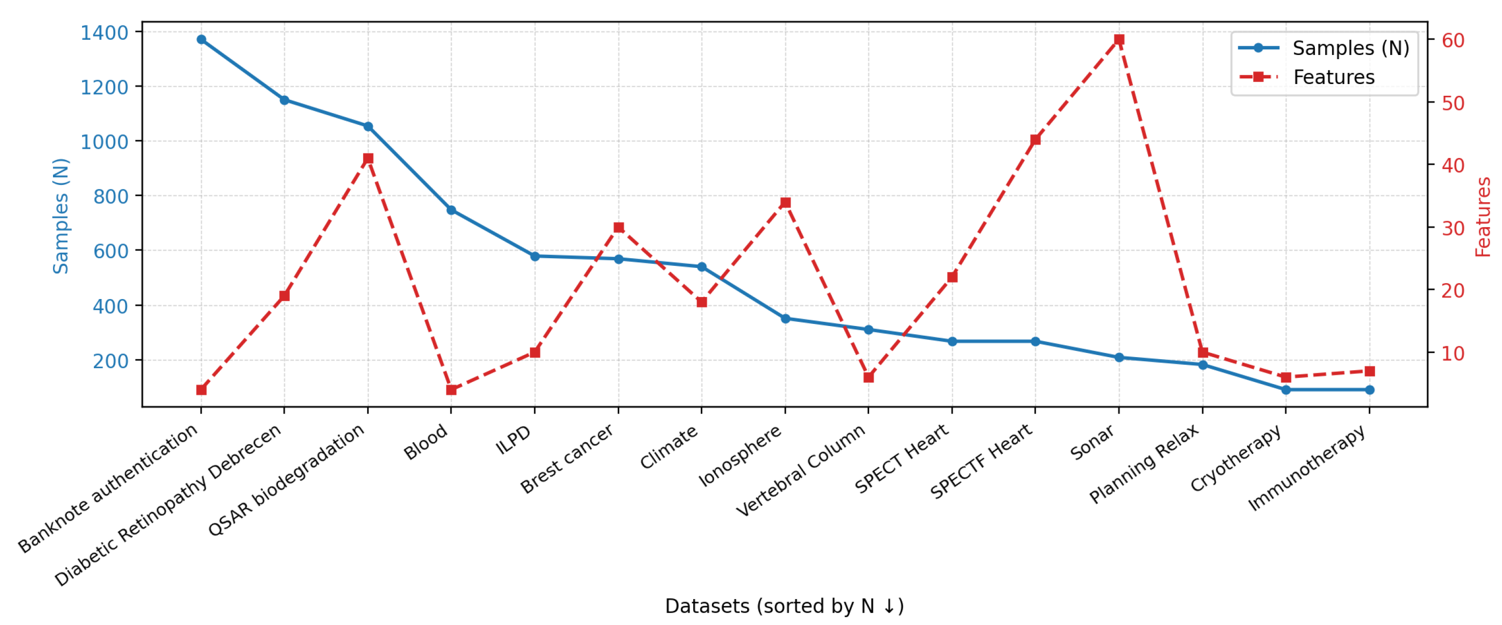
Figure 2.
Overview of the SGNN methodology, from left to right. Input data from different modalities (numerical, categorical, imaging, high-frequency signals, and EHR) is processed by an ensemble of low-dimensional classifiers (LDCs), each trained on a pair of features using class labels. Class boundaries (e.g., red/green lines) are learned via standard ML kernels such as SVMs. The outputs of these classifiers define edge weights in the Synolitic graph. Synolitic graph is classified by GNN of two possible architectures, leading to the result.
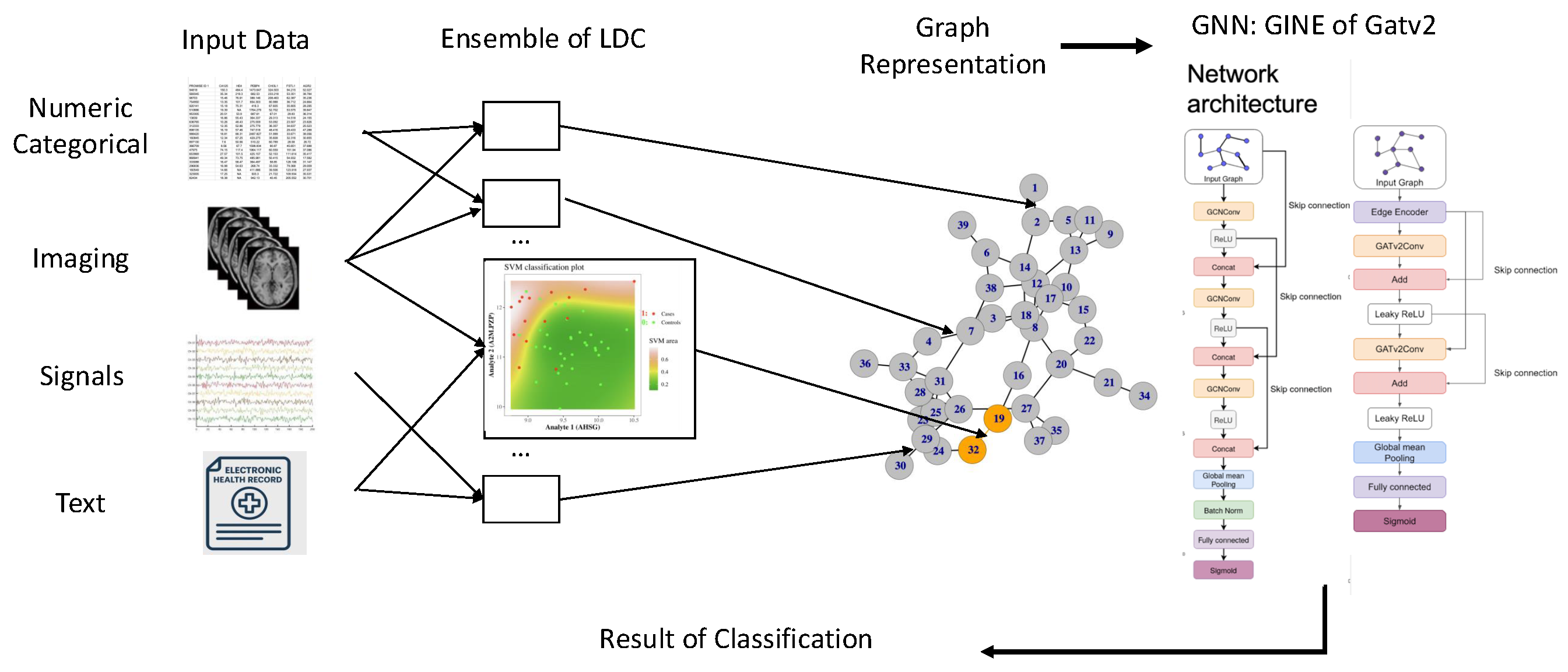
Figure 3.
Performance comparison between SGNNs and conventional machine learning models under varying training set sizes. ROC-AUC estimation vs the size of the training data (taken as a fraction from the original number of samples). For each dataset, the size of the training set was systematically reduced below 20% to assess robustness in low-sample regimes. Standard models such as XGBoost exhibited a marked decline in classification performance, while the SGNN pipeline maintained strong generalisation, achieving ROC-AUC scores above 80% compared to approximately 63% for XGBoost. These results demonstrate the superior ability of SGNNs to overcome the curse of dimensionality and perform reliably in high-dimensional, small-sample datasets.
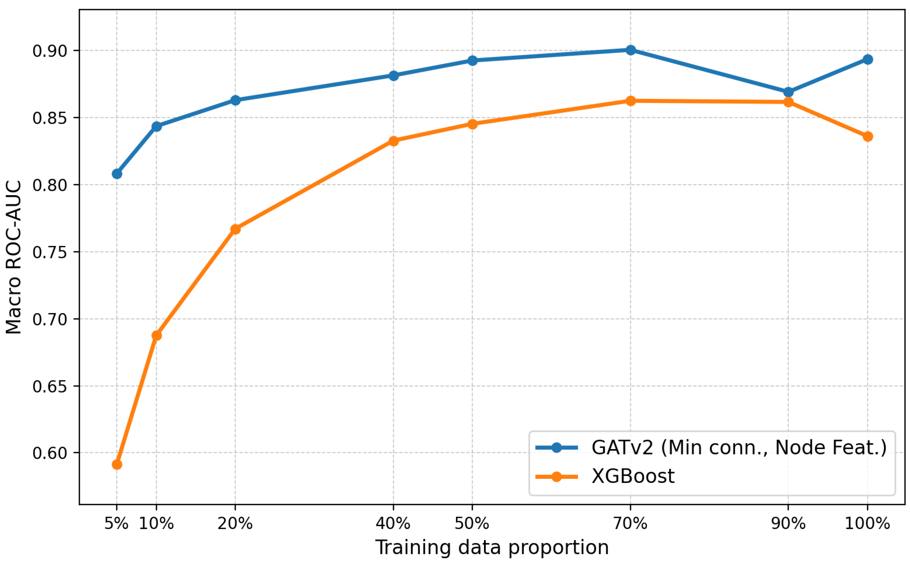

Table 1.
Configuration parameters for the Graph Neural Networks.
| Parameter | Value | Parameter | Value |
|---|---|---|---|
| GNN Model Parameters | |||
| Activation function | Leaky ReLU | Hidden layer size | 128 |
| Number of GNN layers | 2 | Dropout rate | 0.3 |
| Residual connections | True | Use edge encoder | True |
| Edge encoder hidden size | 32 | Number of edge encoder layers | 2 |
| Classifier MLP hidden size | 32 | Number of classifier MLP layers | 2 |
| GATv2 Specific Parameters | |||
| Number of attention heads | 3 | Concatenate head outputs | True |
| Training Configuration | |||
| Learning rate | Batch size | 512 | |
| Maximum epochs | 256 | Early stopping patience | 128 |
| Learning rate patience | 32 | Cross-validation folds | 3 |
| Weight decay | LR reduction factor | 0.5 | |
| Optuna Hyperparameter Optimization | |||
| Number of trials | 8 | Startup trials | 1 |
| Warmup steps | 4 | ||
| XGBoost Baseline Configuration | |||
| Maximum depth | 6 | Learning rate | 0.1 |
| Number of estimators | 100 | Subsample ratio | 0.8 |
| Column sampling ratio | 0.8 | ||
Table 2.
ROC-AUC results in the foundation model setting for different models and sparsification strategies, with and without node features. The caption "Node Features = True or False" means whether the node features were includes or only edge weights were analysed.
Table 2.
ROC-AUC results in the foundation model setting for different models and sparsification strategies, with and without node features. The caption "Node Features = True or False" means whether the node features were includes or only edge weights were analysed.
| Model | Sparsify | ROC-AUC | |
|---|---|---|---|
| Node Feat. = False | Node Feat. = True | ||
| GCN | None | 85.65 | 92.34 |
| p=0.2 | 86.55 | 90.58 | |
| p=0.8 | 85.36 | 90.83 | |
| Min conn. | 85.63 | 91.04 | |
| GATv2 | None | 90.80 | 92.83 |
| p=0.2 | 91.01 | 91.22 | |
| p=0.8 | 90.47 | 92.39 | |
| Min conn. | 90.25 | 91.28 | |
| XGBoost | None | 90.80 | |
Table 3.
Macro ROC-AUC, i.e., averaged over all data-sets, results in the separate datasets setting for different models and sparsification strategies, with and without node features.
Table 3.
Macro ROC-AUC, i.e., averaged over all data-sets, results in the separate datasets setting for different models and sparsification strategies, with and without node features.
| Model | Sparsify | Macro ROC-AUC | |
|---|---|---|---|
| Node Feat. = False | Node Feat. = True | ||
| GCN | None | 84.91 | 87.77 |
| p=0.2 | 80.49 | 83.11 | |
| p=0.8 | 79.06 | 81.84 | |
| Min conn. | 82.43 | 86.17 | |
| GATv2 | None | 86.37 | 88.35 |
| p=0.2 | 87.23 | 86.33 | |
| p=0.8 | 87.20 | 88.68 | |
| Min conn. | 85.80 | 88.96 | |
| XGBoost | None | 86.84 | |
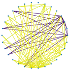
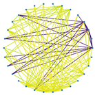
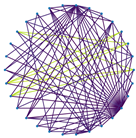
Table 4.
Examples of threshold-based edge sparsification: fully connected graph, top 20% strongest edges, and minimum connected graph. Rows correspond to samples with positive (True) and negative (False) labels.
Table 4.
Examples of threshold-based edge sparsification: fully connected graph, top 20% strongest edges, and minimum connected graph. Rows correspond to samples with positive (True) and negative (False) labels.
| Fully connected graph | Top 20% most significant edges | Max threshold preserving connectivity | |
|---|---|---|---|
| Label = True | 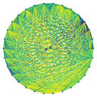 |
 |
 |
| Label = False | 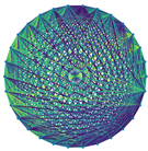 |
 |
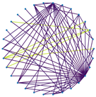 |
Table 5.
Effect of SGNN sparsification and node feature augmentation on macro ROC-AUC.
| Configuration | ROC-AUC |
|---|---|
| Synolitic graph only | 70.34 |
| Sparsified at maximum threshold while remaining connected | 71.07 |
| With additional node features | 78.39 |
Table 6.
Models trained with the current baseline parameters. The evaluation metric is the macro-averaged AUROC across all tasks. Each cell in the table shows the AUROC values for the original and noise-augmented datasets, separated by a “/” symbol, respectively. The better value within each pair is underlined, while the overall best performance across all configurations is highlighted in bold. It can be observed that, for some tasks, performance actually improves with the addition of noise. However, in other cases, the metric decreases more noticeably compared to the boosting model, whose performance remains higher than that of certain configurations.
| Model | Sparsify | Macro ROC-AUC | |
|---|---|---|---|
| Node Feat. = False | Node Feat. = True | ||
| GCN | None | 84.91 / 77.40 | 87.77 / 84.01 |
| p=0.2 | 80.49 / 78.53 | 83.11 / 83.02 | |
| p=0.8 | 79.06 / 80.70 | 81.84 / 86.73 | |
| Min conn. | 82.43 / 83.41 | 86.17 / 85.57 | |
| GATv2 | None | 86.37 / 87.36 | 88.35 / 87.93 |
| p=0.2 | 87.23 / 85.60 | 86.33 / 88.44 | |
| p=0.8 | 87.20 / 81.71 | 88.68 / 87.38 | |
| Min conn. | 85.80 / 82.74 | 88.96 / 88.82 | |
| XGBoost | None | 86.84 / 85.90 | |
Disclaimer/Publisher’s Note: The statements, opinions and data contained in all publications are solely those of the individual author(s) and contributor(s) and not of MDPI and/or the editor(s). MDPI and/or the editor(s) disclaim responsibility for any injury to people or property resulting from any ideas, methods, instructions or products referred to in the content. |
© 2025 by the authors. Licensee MDPI, Basel, Switzerland. This article is an open access article distributed under the terms and conditions of the Creative Commons Attribution (CC BY) license (http://creativecommons.org/licenses/by/4.0/).
Copyright: This open access article is published under a Creative Commons CC BY 4.0 license, which permit the free download, distribution, and reuse, provided that the author and preprint are cited in any reuse.


