Submitted:
28 November 2025
Posted:
02 December 2025
You are already at the latest version
Abstract
Multiple Instance Learning (MIL) is a standard paradigm for classifying gigapixel whole-slide images (WSIs). However, prominent models such as Attention-Based MIL (ABMIL) treat image patches as independent instances, ignoring their inherent spatial context. More advanced frameworks like MuRCL employ reinforcement learning for instance selection but do not explicitly enforce spatial coherence, often resulting in noisy localizations. Although Graph Neural Networks (GNNs), attention smoothing, and reinforcement learning (RL) are each powerful, state-of-the-art strategies for addressing these issues individually, their integration remains a significant challenge. This paper introduces SG-MuRCL, a framework that enhances MuRCL by first employing a GNN to model spatial relationships—departing from ABMIL’s independence assumption—and second incorporating an attention-smoothing operator to regularize the MIL aggregator, aiming to improve robustness by generating more coherent and clinically meaningful heatmaps. Empirical evaluation yielded an important finding: while the baseline MuRCL trained successfully, the integrated SG-MuRCL consistently collapsed into a trivial solution. This outcome shows that the theoretical synergy between GNNs, attention smoothing, and RL does not trivially translate into practice. The contribution of this work is therefore not a high-performing model, but a concrete demonstration of the scalability and stability challenges that arise when unifying these advanced paradigms.
Keywords:
computational pathology
; whole slide image analysis
; multiple instance learning
; graph neural networks
; attention smoothing
; reinforcement learning
; contrastive learning
; self-supervised learning
; weak supervision
; interpretability
; CAMELYON16
1. Introduction
Digital pathology has moved from glass slides to whole slide images that capture tissue at very high resolution. This shift has opened a path for computational support in diagnosis and research, yet it also brings practical obstacles. Whole slide images are too large for direct processing with conventional convolutional networks, and the lack of pixel level labels makes fully supervised learning impractical at scale [1,2]. Multiple instance learning has therefore become a natural choice. In this setting a slide is divided into many small patches that form a bag, and supervision is provided only at the bag level [3]. Attention based multiple instance learning has helped identify which patches are most informative, but most methods still treat patches as independent and often rely on heuristic selection, which can discard subtle but clinically important regions [4,5]. These choices limit both accuracy and the coherence of heatmaps used for interpretation [6,7].
The clinical motivation is clear. Reliable slide level classifiers can support triage, reduce variability among readers, and focus attention on suspicious regions. Studies in prostate biopsy grading already show that assistance from artificial intelligence can improve agreement with subspecialists and streamline review [8,9] . At the same time, weak supervision and strong inter center variability make generalization difficult. Differences in staining, scanners, and patient populations amplify the risk of overfitting [10,11]. Methods that acknowledge spatial context while remaining trainable at whole slide scale are still needed.
Multi Instance Reinforcement Contrastive Learning, or MuRCL, moves the field forward by coupling reinforcement learning for patch selection with contrastive learning for representation learning [12]. MuRCL improves how informative regions are chosen, yet it does not explicitly encode spatial relationships among patches and it does not regularize attention to produce smoother and more clinically faithful heatmaps. We explore these two gaps.
In practical terms, MuRCL can still attend to isolated patches that are individually discriminative but spatially incoherent, and it cannot enforce that neighbouring regions with similar morphology receive similar importance. Moreover, the CNN backbone used in MuRCL is agnostic to the explicit topology of the slide and operates on patches as independent inputs. SG-MuRCL was therefore designed to address these limitations by (i) inserting a graph neural network between the frozen CNN encoder and the MIL aggregator to propagate information across spatial neighbours, and (ii) adding an attention-smoothing operator to explicitly penalize fragmented, noisy attention patterns at the slide level.
Our study asks a single question: can explicit spatial modeling with graph neural networks and attention smoothing, when integrated into MuRCL, improve accuracy, robustness, and localization quality on whole slide images without unacceptable computational cost?
We make three contributions. First, we reproduce MuRCL on CAMELYON16 and report a transparent baseline that others can compare against. Second, we design SG MuRCL, which combines a graph attention encoder to model spatial relations with a smoothed transformer based attention pooling module, while keeping the reinforcement learning selector and contrastive objective. Third, through systematic experiments we find that this integrated design exposes severe training instabilities that lead to collapse, and we analyze why this happens in practice. The result is a clear account of what works, what fails, and what the community may need to solve before complex spatial and selection mechanisms can be safely deployed at whole slide scale.
2. Related Work
MIL has emerged as a powerful framework for medical image classification, such as WSIs, particularly in digital pathology where only slide-level or patient-level labels are available. This framework divides the WSI into numerous smaller patches (instances), which are collectively labeled with the available slide label (bag). Early MIL methods largely focused on instance-level classification, where each instance is classified independently and then aggregated to determine the final decision. Although straightforward, this ignores potential interactions among instances that may be crucial for a precise diagnosis [1,13,14].
To address this shortcoming, embedding-level MIL approaches emerged, training neural networks to encode instances into a joint feature space. Here, the relative importance of each instance can be modeled either implicitly through shared embeddings or explicitly through attention mechanisms [4]. Beyond standard attention, more advanced strategies have sought to impose additional structure. For example, clustering-based MIL groups visually similar patches to form semantically meaningful concepts, but often does so at the cost of disregarding their crucial spatial arrangement within the tissue architecture [15]. Hierarchical MIL, on the other hand, processes information at multiple scales (e.g., from patches to regions) like Cersovksy et al. and Wu et al. [16,17], but can introduce significant computational complexity and often relies on heuristic region-defining strategies.
2.1. Attention-Based MIL
Attention-based MIL has received considerable attention because it not only identifies the most discriminatory instances but also offers greater interpretability by highlighting the regions most responsible for the final prediction of the model. Despite these benefits, attention-based approaches frequently treat each instance independently, ignoring how neighboring or distant instances might influence each other [6]. This can be problematic in histopathology, where subtle morphological patterns, such as gradual transitions from healthy tissue to early-stage malignancy, may only become apparent when viewed within the broader tissue environment.
2.2. Transformer-Based MIL
Transformer-based MIL extends the concept of attention to the global scale, utilizing self-attention to capture long-range interactions between instances [18,19]. Rather than computing attention scores for each instance, the transformer compares each instance with all other instances in a bag. In principle, this method can capture intricate spatial correlations over wide tissue regions. In practice, however, the computational expense of self-attention growing quadratically with the number of instances makes it prohibitive for WSIs containing tens or even hundreds of thousands of patches. Researchers have proposed different down-sampling or hierarchical schemes [20,21] to mitigate this complexity, but these strategies can still cause critical fine-grained details to be lost if sampling is too coarse or heuristic-driven. Hence, while transformer-based solutions excel in capturing global context, they remain difficult to deploy on extremely large WSIs without discarding valuable local information.
2.3. Local-Global Modeling Strategies
While transformers excel at capturing global context, their computational cost has spurred the development of alternative strategies that seek to model both local and global dependencies more efficiently. One intuitive approach is to use multi-scale networks that process instances at different resolutions. For example, Li et al. [22] and Wu et al. [17] proposed dual-stream networks that separately encode coarse-resolution instances for large-scale context and fine-resolution instances for intricate detail. While effective, these methods can require exhaustive instance processing and tremendous computational resources.
Another approach has been to adapt traditional Convolutional Neural Networks (CNNs) by incorporating spatial attention mechanisms. These models can learn to weight local regions differently but often struggle to model long-range dependencies explicitly and are sensitive to the rotation and translation of tissue structures due to their fixed kernel structures.
More recently, Vision Transformers (ViTs) have been adapted for WSI analysis. A prominent example, TransMIL [18], treats the WSI as a sequence of patch embeddings. However, this sequentialization often disrupts the native 2D spatial topology of the tissue. Recognizing this limitation, other works like HIPT [21] have proposed hierarchical ViT structures to better preserve local spatial context before modeling global relationships, acknowledging the inherent challenge of applying standard transformers to this domain.
2.3.1. GNN-Based MIL
In contrast to the methods above, GNNs offer a more natural and powerful solution for local-global modeling in pathology [23]. By representing patches as nodes in a graph connected by edges based on spatial proximity, GNNs are uniquely suited to respect the underlying tissue architecture. This graph structure allows for explicit, iterative message passing between adjacent instances, effectively propagating local information throughout the entire WSI.
This makes GNNs particularly suitable for modeling tissue morphology for several reasons. Unlike CNNs, they are inherently permutation-invariant and can naturally model the irregular, non-grid-like structure of tissue sections. Unlike ViTs that sequentialize data, GNNs explicitly leverage the 2D neighborhood relationships. GNN-based MIL can thus unify local cellular details with a global tissue overview while reducing potential noise from isolated artifacts. However, like other advanced methods, GNNs also require large computational resources to build and process large graphs, emphasizing the need for efficient sampling or subgraph selection strategies, a challenge our RL-based framework is designed to address.
2.3.2. Sm: Smoothing Operator
Despite advancements in GNNs and AB-MIL, instance-level predictions remain prone to noise and inconsistencies, which can hinder accurate lesion localization. Variations in staining protocols, imaging artifacts, and the inherent challenge of boundary detection contribute to erratic predictions, leading to discontinuities in malignancy scores that conflict with the expected morphological continuity of tissue structures. To mitigate this, Castro-Macías et al. Castro-Macias et al. [6] proposed a smoothing mechanism that enforces local consistency among neighboring instances. This approach ultimately enhances both diagnostic accuracy and interpretability in clinical settings, making it a valuable tool for lesion localization in medical imaging. That said, like the aforementioned frameworks its computational cost raises concerns. It scales with the bag size posing a considerable challenge for WSI analysis.
2.4. RL in WSI
Recognizing that instance selection is of utmost importance to mitigate computational overhead, some researchers have employed simple heuristics to remove irrelevant instances. These strategies, however, risk excluding subtle tumor foci similar to healthy tissue. Consequently, RL gained a surge of interest in reformulating instance selection as a sequential decision-making process [5,12,24]. By rewarding correct classification or similarity to expert annotations, a RL agent can iteratively learn to focus on the most relevant regions [25]. Yet, many existing RL-based solutions emphasize instance selection in isolation, neglecting the value of simultaneously accounting for local-global dependencies once the selected instances are passed to a downstream classifier like MIL. A related line of work outside pathology further demonstrates that reinforcement-learning-based MIL can be effective in domains with smaller bags and more homogeneous instance distributions. For example, Lakeman et al. [26] proposed a reinforcement-driven MIL framework for multi-task speaker attribute prediction, showing that RL-based instance selection can stabilize when operating on lower-dimensional, non-spatial data. This contrast highlights that the extreme scale and spatial heterogeneity of WSI bags pose additional challenges that are not present in other MIL domains.
3. Methodology
The research detailed in this paper follows a constructive methodology. We begin by designing and implementing a novel deep learning framework, SG-MuRCL, which enhances an existing state-of-the-art model to address specific and well-defined limitations. Subsequently, we conduct a rigorous quantitative and qualitative experimental evaluation to validate the proposed enhancements and measure their impact on model performance, generalization, and interpretability. The core problem we address is twofold: 1) standard MIL models often assume statistical independence between patches, disregarding the crucial spatial context inherent in tissue architecture; and 2) the attention mechanisms used for MIL aggregation can produce noisy, fragmented heatmaps that limit clinical utility.
In designing SG-MuRCL, we treated “generality” and “interpretability” as concrete, measurable design objectives rather than purely qualitative aspirations. Generality is understood as robustness of the learned encoder and policy to changes in graph construction and RL configuration, which can be probed through sensitivity to parameters such as the spatial radius_ratio, the number of clusters in the action space, and the number of selected instances k. Interpretability is associated with properties of the resulting attention maps that can be quantified, for example, by attention entropy, spatial continuity measures, and the total-variation of attention over the slide. Even though the full model ultimately collapsed, these criteria guided our architectural choices and the subsequent failure analysis.
3.1. SG-MuRCL Framework
The proposed solution is to extend the MuRCL framework [12] by integrating two key architectural innovations. First, we incorporate GNNs to explicitly model spatial relationships between tissue patches. Second, we leverage a smoothing operator, inspired by the work of Pereira et al. and Castro-Macías et al., respectively [6,7], within the MIL aggregator and Transformer to enforce local and global predictive consistency. The resulting SG-MuRCL pipeline operates as a self-supervised pretraining regime designed to learn robust WSI representations without requiring patch-level annotations. The framework can be conceptually divided into an offline data preparation phase and an online training phase. Figure 1 describes the overall pipeline.
3.1.1. Offline Data Preparation
This initial, offline data preparation phase transforms each raw WSI into a structured data format, a crucial prerequisite for the graph-based and RL approach. The process begins by identifying and filtering for relevant tissue regions, which are then systematically tiled into a collection of smaller, fixed-size image patches, with the precise coordinates of each patch being recorded for subsequent spatial analysis. Next, each patch is processed by ResNet18 and ResNet50 [27] pretrained on ImageNet. These embeddings and coordinates form the basis for the final structured representation. A spatial graph is constructed where the patches serve as nodes and the edges connect them based on physical proximity, capturing the architecture of the local tissue. Alternatively, a KNN graph can be built on feature similarity to connect visually similar patches regardless of location. Finally, to define a tractable and semantically meaningful action space for the RL agent, K-Means clustering is applied to the patch embeddings, grouping them into a set of discrete clusters based on similarity.
3.1.2. Spatial Patch-Graph Construction
In this framework, each WSI is structured as a patch-graph where each node corresponds to a tissue patch, and the edges represent their spatial relationships on the slide similar to [7]. To define these relationships, we implement an adaptive spatial graph construction method based on radius connectivity.
Let the set of coordinates for all N patches in a given WSI be denoted as , where each coordinate . Instead of using a fixed-distance radius for all WSIs, which may not be optimal for varying tissue sizes, we calculate a dynamic radius for each slide individually. This radius is determined as a fraction, (the `radius_ratio`), of the maximum spatial spread of the tissue patches. Formally, the radius is calculated as:
This adaptive approach ensures that the connectivity scale is appropriate to the specific topology of each WSI. An edge is then established between any two nodes, i and j, if the Euclidean distance between their corresponding patches, , is less than or equal to this calculated radius . This results in a symmetric adjacency matrix , where:
This implementation ensures that every node is connected to itself (i.e., ), guaranteeing self-loops in the graph.
Finally, for compatibility with modern graph deep learning libraries, this dense adjacency matrix is converted into the standard sparse `edge_index` format. This format is a tensor of shape , where E is the total number of edges. Each column in this tensor represents an edge by storing the indices of the source and target nodes. This sparse representation is computationally efficient and is the final input used by the GNN model.
3.1.3. Online Pretraining
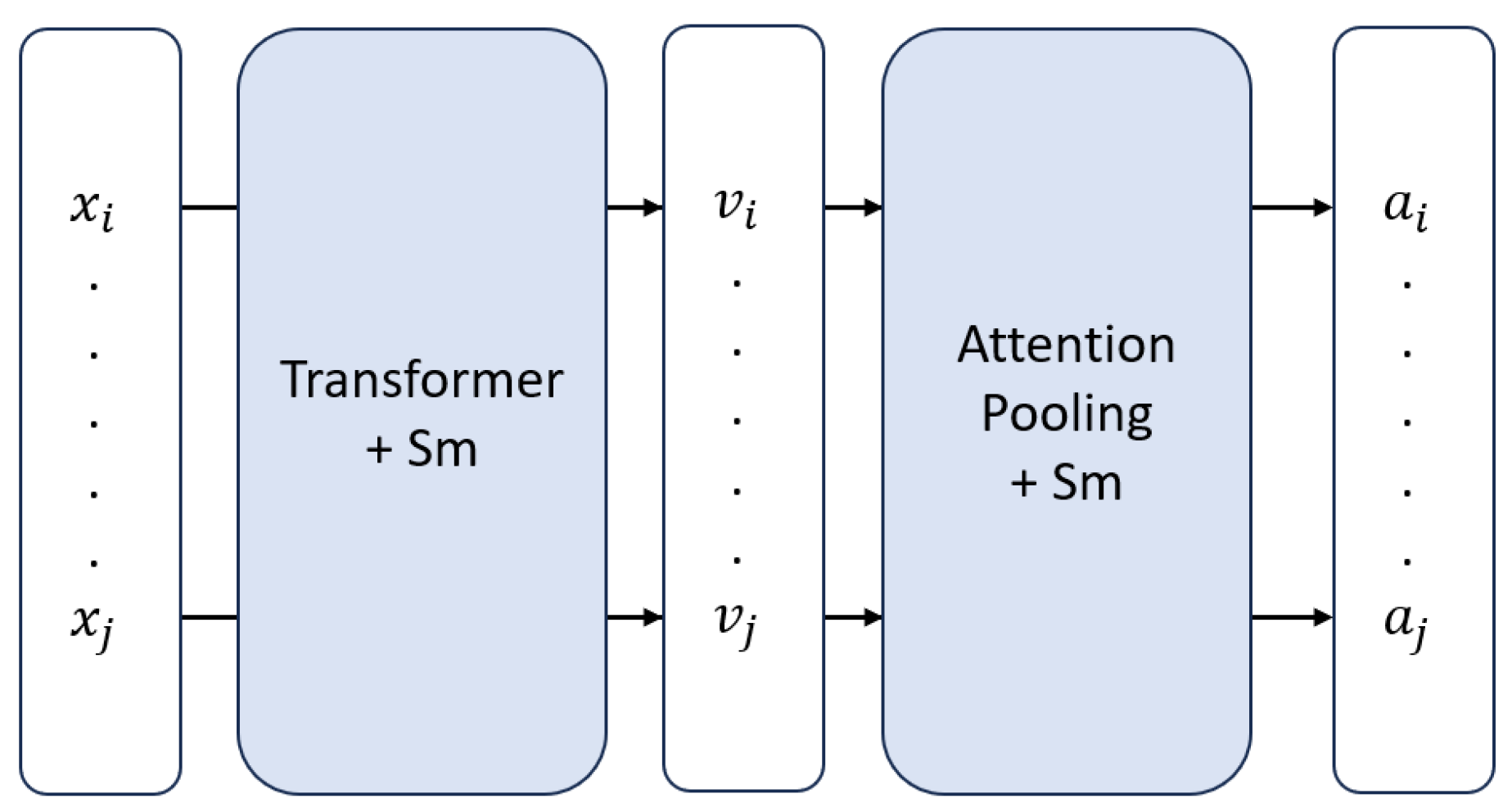
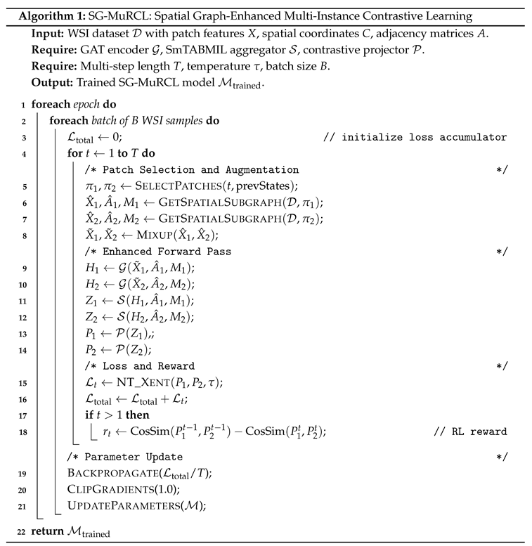
The core training loop is driven by a contrastive learning objective, which learns by comparing two distinct "views" generated from the same WSI. These views are created by two parallel RL-MIL branches. Within each branch, an RL agent iteratively selects a subset of patches. The features of these selected patches are immediately refined by a Graph Attention Network (GAT), which produces context-aware embeddings by aggregating information from neighboring patches in the subgraph. These refined embeddings are then passed to the Smoothed Transformer ABMIL (SmTAP) [6] aggregator, where a smoothing operator encourages spatially coherent attention scores during the creation of a final, slide-level bag embedding. Figure 2 shows a high-level overview of this setup. We train the encoder with the temperature-scaled NT-Xent loss [28]. NT-Xent is preferred to triplet or margin losses because it: (i) uses every other patch in the mini-batch as a negative, giving a richer signal for the highly variable WSI domain; (ii) includes a temperature that smooths gradients and prevents collapse; and (iii) avoids hard-negative mining, which is unreliable under weak slide-level supervision. A single NT-Xent term drives the whole pipeline, while the RL agent is rewarded whenever its patch selections improve the positive-vs-negative separation, encouraging discovery of diverse, informative regions. Pseudo code is provided below.
Figure 2.
High-level overview of SmTAP. Here, and denote instances, and are their corresponding feature embeddings, and and are the attention values assigned to each instance.
Figure 2.
High-level overview of SmTAP. Here, and denote instances, and are their corresponding feature embeddings, and and are the attention values assigned to each instance.
3.1.4. Supervised Finetuning
After the self-supervised pretraining phase, the learned encoder and the RL selection policy are adapted for a specific downstream classification task. The contrastive projection head is replaced with a new, randomly initialized classification layer. The entire model is then fine-tuned on a labeled dataset using a Cross-Entropy loss function. During this fine-tuning stage, the reward mechanism for the RL agent is re-calibrated. Instead of being rewarded for representational diversity, the agent is now rewarded for selecting subsets of patches that increase the model’s predictive confidence. This crucial step adapts the exploratory policy learned during pretraining into a highly discriminative policy, optimizing the patch selection process specifically for classification accuracy. This multi-stage process allows the model to first learn a rich, general understanding of tissue morphology and then specialize this knowledge to a targeted diagnostic task.
3.2. Evaluation
The proposed framework is evaluated against MuRCL serving as a baseline, enabling the quantification of improvements in both classification and generalization capabilities [12]. Performance metrics such as accuracy (ACC), area under the curve (AUC), precision, recall, and the F1 score are used to ensure a comprehensive assessment of the model. ACC offers a straightforward measure of the proportion of correctly classified slides, while AUC is especially valuable because it captures the model’s capability to distinguish positive from negative slides independent of a fixed classification threshold. Precision and recall metrics are crucial for medical diagnostics, as they quantify, respectively, the reliability of positive predictions and the model’s sensitivity to detecting true positive instances. The F1 score provides a balanced metric, combining precision and recall into a single value particularly useful when dealing with imbalanced datasets common in clinical scenarios.
3.3. Experimental Setup
3.3.1. Dataset Overview
To rigorously evaluate the proposed SG-MuRCL framework, we selected the CAMELYON16 dataset [29] as the primary benchmark. This dataset is widely regarded as a gold-standard for evaluating models on the task of detecting lymph node metastasis in breast cancer WSIs. Its composition of 399 WSIs (270 for training, 129 for testing) sourced from two distinct medical centers (RUMC and UMCU) provides a realistic level of inter-center variability, making it an excellent testbed for model robustness. All experiments were standardized to the 20x magnification level to ensure consistency across the dataset.
A multi-stage pre-processing pipeline was implemented to transform the raw gigapixel-sized WSIs into a format suitable for graph-based deep learning. This process follows established best practices in the field [22,30]. First, each WSI was tiled into non-overlapping 256x256 pixel patches. This patch size was chosen to balance the capture of fine-grained cellular detail with manageable computational requirements. Subsequently, a crucial tissue segmentation step was performed to eliminate non-diagnostic background regions, such as glass and pen markings. This was achieved by converting each patch to the RGB color space and applying a threshold to the saturation channel, a robust method for identifying areas rich in stained tissue. Any patch with less than 35% tissue content was discarded, allowing the model to focus its computational resources on the most informative parts of the slide.
Finally, to facilitate hyperparameter optimization and prevent overfitting, the official CAMELYON16 training set of 270 slides was partitioned. 80% of these slides were allocated for model training, while the remaining 20% were held out as a dedicated validation set. Upon completion of this pipeline, the processed dataset comprised approximately 2.75 million individual patches, grouped into "bags" corresponding to each WSI, with an average bag size of 6882 patches per slide. This large bag size underscores the computational and methodological challenges that MIL frameworks are designed to address. Figure 3 shows how the patch distribution is over both training and test data.
3.3.2. Implementation Details
Patch-level feature representations were generated using ResNet18 and ResNet50 backbones, pretrained on ImageNet [27]. The SG-MuRCL implementation utilized a two-layer GAT for graph-based processing. A deeper GNN was deliberately avoided because preliminary profiling indicated that adding further layers on WSI-scale graphs dramatically increased memory consumption and led to pronounced over-smoothing of node embeddings, a well-known failure mode in GNNs. A two-layer configuration therefore represented the deepest architecture that remained compatible with our GPU memory constraints while still expanding the receptive field beyond immediate neighbors in a controlled way. The reinforcement learning agent was configured to select a subgraph of k=512 instances from each WSI, with its action space defined by 10 clusters generated via K-Means. For experiments involving attention smoothing, the operator’s standard deviation was set to 1.0.
To establish a robust baseline and ensure a fair comparison, the implementation adopted the core hyperparameters from the original works that introduced the key components of the framework [6,7,12] wherever possible. Specifically, all models were trained using the Adam optimizer with an initial learning rate of and a weight decay of . A batch size of 128 was used throughout all experiments. The self-supervised pretraining phase was run for 100 epochs. For the subsequent supervised fine-tuning stage, models were trained for a maximum of 50 epochs, utilizing an early stopping mechanism that monitored validation performance with a patience of 10 epochs. All experiments were conducted on a cluster of 4 NVIDIA A100 GPUs. A list of all settings and hyperparameters can be found in the Appendix A.
4. Results
This section first establishes a reproducible MuRCL baseline on CAMELYON16 using standard classification metrics. We then present the behavior of the proposed SG MuRCL under the same protocol, highlighting training dynamics and the observed collapse to a trivial decision rule. We also summarize the computational profile at inference and a simple stability indicator from the training trajectory. Together these results show what is reliably achievable and where the integrated design breaks down in practice.
4.1. Baseline Performance of MuRCL
To quantify the impact of our proposed SG-MuRCL framework, we first established a performance baseline by implementing the original MuRCL architecture [12]. These experiments evaluate the baseline’s effectiveness with three different feature extraction backbones. The final performance metrics on the CAMELYON16 test set are presented in Table 1.
The quantitative results show a clear performance hierarchy among the tested configurations. The ResNet50 (ImageNet) backbone yielded the most effective performance in our setup, achieving an AUC of 0.754 and an F1-score of 0.610. Notably, these results are substantially lower than those reported in the original MuRCL publication, a critical finding that will be thoroughly analyzed in Section 5.
To provide a deeper understanding of the training dynamics that produced the results in Table 1, Figure 4 shows the progression of loss, accuracy, and AUC for the training, validation, and test sets.
This confirms that the scores reported represent the models’ peak capabilities under our experimental conditions, rather than being artifacts of premature termination. Furthermore, the significant gap between the training curves and the validation/test curves across all configurations highlights the inherent difficulty of the task and the degree of overfitting, a key challenge that our proposed SG-MuRCL framework is designed to address. A detailed analysis comparing these results to the state-of-the-art and exploring the performance discrepancy is reserved for the Discussion Section 5 section.
4.2. Experimental Performance of SG-MuRCL
In contrast to the stable training of the baseline, our implementation of the SG-MuRCL framework encountered critical instabilities during the training process. Despite significant efforts in implementation and debugging, the integrated model consistently failed to learn a meaningful classification policy. For all tested encoders, the framework rapidly converged to a trivial solution where it predicted the majority class for every sample in the test set. This outcome is a key finding of our research. The performance metrics, shown in Table 2, are a direct reflection of this training collapse. Qualitatively, intermediate checkpoints from the early stages of SG-MuRCL training did produce smoother and more spatially contiguous attention patterns than the baseline MuRCL, consistent with the intended effect of the SmTAP module that we illustrate explicitly on MuRCL in Figure A1. However, because SG-MuRCL does not converge and collapses shortly thereafter, we chose not to present these early attention maps as central quantitative evidence. Instead, they are used internally to verify that the smoothing mechanism itself behaves as designed before the joint optimization of all components becomes unstable. The accuracy of 0.620 matches the proportion of negative samples in the test set, the auc of 0.500 indicates a complete lack of discriminative ability, and the F1-score of 0.000 confirms the failure to identity any positive instances. The consistency of this failure across different encoders suggests the issue is systemic to the complexity of the integrated framework itself. A thorough analysis of the underlying challenges is presented in the Discussion Section 5.
In addition to the summary metrics in Table 2 and Table 4 and the loss trajectories in Figure 5, we monitored several internal signals during training. First, the gradient norms of the main network parameters quickly decayed towards very small values after only a few epochs in SG-MuRCL, in contrast to the baseline MuRCL where gradients remained well-behaved. Second, the attention distributions in the MIL aggregator moved towards near-uniform patterns, as reflected by a rapid drop in attention entropy, indicating that the model stopped discriminating between patches. Finally, the cosine similarities used in the contrastive loss converged to almost constant values across batches. Together, these diagnostics support the interpretation that the model settled into a trivial stationary point rather than learning meaningful slide-level representations.
4.3. Computation Complexity
Beyond classification performance, a key consideration for clinical deployment is the computational cost at inference time. To quantify the overhead of our proposed architectural enhancements, we measured the average time required for a model to perform a single forward pass on a pre-processed WSI. This measures the latency of the core model architecture, excluding the offline data preparation steps. The results, using the ResNet50 backbone on an NVIDIA A100 GPU, are presented in Table 3.
The table clearly illustrates the practical trade-offs of our design. While the MuRCL baseline is relatively efficient, our proposed SG-MuRCL framework, with its graph-based computations, nearly triples the inference time. This demonstrates that the architectural choices designed to improve robustness and interpretability come at a significant, practical price in terms of deployment feasibility and speed, a critical factor for real-world clinical applications.
As illustrated in Figure 5 and summarized in Table 4, the extremely low loss variance of SG-MuRCL might counter-intuitively suggest a stable model. However, this interpretation is misleading and reveals the opposite. The higher variance of the baseline model (0.001279) reflects a successful and dynamic learning process, where the loss starts high and consistently decreases as the model learns, thus covering a wider range of values.
In stark contrast, the zero variance of the SG-MuRCL model (0.000000) is quantitative proof of its training collapse. The model immediately becomes trapped in a poor local minimum. The trivial solution of predicting the majority class, and fails to explore the loss landscape. Its loss remains nearly constant at a high value, resulting in minimal variance. This metric provides strong, direct evidence that the framework’s instability prevented any meaningful learning from occurring.
5. Discussion
This section interprets the empirical findings and explains why the baseline is stable yet below reports in the literature while the integrated SG MuRCL fails to learn. We examine interactions among modules, sensitivity to graph construction and policy design, and constraints imposed by memory and batch size. We then draw practical lessons for method selection in pathology, outline changes that could make similar systems tractable, and point to directions for future work.
5.1. Comparison with State-of-the-Art
Our initial objective was to establish a robust performance baseline by implementing the original MuRCL framework [12]. As shown in Table 1, our implementation produced stable and reproducible results, with the ResNet50-ImageNet encoders achieving the best performance. However, there is a substantial discrepancy when comparing this to the results reported in the original publication. This performance gap is a common challenge in replicating complex deep learning studies and likely stems from a combination of factors.
Key among these are subtle but critical differences in experimental conditions that are often omitted from papers for brevity. This includes the exact parameters of the optimizer, the nature of any learning rate schedules, and, most importantly, the use of data pre-processing techniques like stain normalization, which we did not implement. Furthermore, the performance of any MIL model is critically dependent on the quality of its pretrained feature extractor; minor variations in the backbone’s training protocol can lead to significant downstream performance differences. A pretrained ResNet SimCLR was used. However, these weights were not available to us. While our baseline did not achieve state-of-the-art performance, it successfully served its purpose by validating our experimental environment and providing a stable, internally-consistent benchmark for the more complex experiments that followed. Additionally, the intended effect of the SmTAP can be seen in Figure A1.
Beyond MuRCL, several spatial MIL architectures such as GNN-based MIL models and hierarchical transformer approaches like HIPT have been proposed for WSI classification. Running a full set of experiments with these methods inside our pipeline would require substantial additional compute and engineering effort and was therefore outside the scope of this work. Nevertheless, their published results on CAMELYON16 and related datasets indicate that spatial modeling can be beneficial when deployed in isolation. Our findings should thus not be read as a critique of spatial MIL in general, but as evidence that combining graph propagation, attention smoothing, and reinforcement learning into a single, end-to-end framework introduces a distinct class of stability and scalability issues that is not yet addressed by existing methods. Recent work by Braakman et al. [31] specifically examined the accuracy–interpretability trade-off in RL-based MIL frameworks and similarly reported that reward design and instance-selection dynamics have strong effects on stability. Their findings reinforce our conclusion that RL-guided sampling remains highly sensitive to architectural coupling and initialization. While their work focuses on improving interpretability within RL-MIL, our results show that combining RL with graph propagation and attention smoothing introduces additional gradient interactions that can destabilize training at WSI scale.
Moreover, directly plugging architectures such as GNN-based MIL or HIPT into the MuRCL pipeline is non-trivial, because they were not designed to expose a reinforcement-learning selection policy or a contrastive reward interface compatible with MuRCL’s training dynamics.
5.1.1. System Fragility and Unstable Gradient Flow
The primary issue appears to be the immense fragility of a system with multiple, deeply-interacting learning components. The framework requires the simultaneous optimization of a feature aggregator, a GNN, and an RL agent’s policy. This deep computational graph is highly susceptible to training pathologies like vanishing or exploding gradients. A vanishing gradient, for instance, would mean the reward signal from the contrastive loss was too attenuated to ever update the RL agent’s policy, creating a feedback loop where the agent provides poor subgraphs, the GNN produces non-informative embeddings, and the system can never recover. This "black box" nature of the interacting gradients made it intractable to isolate the precise point of failure, highlighting a significant practical gap between modular theory and stable implementation.
5.1.2. Impact of Encoder Choice
As shown in Table 2, the training collapse was consistent across all encoder backbones. This suggests the failure is systemic to the framework’s architecture, not a specific feature extractor. Counter-intuitively, it is plausible that a more powerful encoder like ResNet50 could exacerbate the instability. A deeper model with more parameters creates a more complex loss landscape, and when combined with the multiple interacting learning components of SG-MuRCL, it may be more prone to falling into a poor local minimum. In this case, the trivial majority-class solution.
5.1.3. Hyperparameter Sensitivity and Initialization
The training collapse was likely exacerbated by the framework’s extreme sensitivity to its initialization and hyperparameters. Our approach attempted to train the entire complex system end-to-end from the start. A more robust initialization strategy, such as pretraining the GNN and RL agent separately before integration, might have guided the model to a more stable region of the parameter space.
Furthermore, the core hyperparameters impose delicate trade-offs. The graph connectivity `radius_ratio` () and the RL action space ( clusters, 512 instances) represent strong structural priors. A slight misconfiguration of these parameters could easily force the model into a suboptimal policy space from which it cannot escape, leading directly to the observed training failure. for example, a graph radius that is too large or an action space that does not match the semantic diversity of the tissue.
Although a full battery of ablation experiments was not feasible due to the memory footprint of WSI-scale graphs, we carried out an analytical, component-wise failure analysis based on intermediate training behaviour. When inspected in isolation at early epochs, the GNN and the smoothing operator both behaved as expected (message passing and attention regularization were numerically stable), and the RL policy updates remained well-defined when the graph and smoothing modules were disabled. Collapse only appeared once all three components were coupled in a single end-to-end optimization loop. This conceptual ablation suggests that the instability is an emergent property of their interaction rather than a pathology of any single module.
Similarly, we observed consistent qualitative sensitivity trends without performing exhaustive sweeps. Increasing the radius_ratio led to denser graphs and noticeably noisier gradients; enlarging the selection size k made RL rewards more volatile; and changing the number of clusters in the action space altered how sharply the policy focused on a small subset of regions. These observations align with known trade-offs in graph-based MIL and support our interpretation that SG-MuRCL operates in a very fragile region of the hyperparameter space, where modest shifts are sufficient to trigger collapse. In many MIL studies, such sensitivities are summarized via box plots over repeated runs and dense sweeps of each parameter; in our case, the memory cost of WSI-scale graph training prevented such exhaustive exploration, so we instead report the most informative qualitative trends and parameter ranges that were practically attainable.
5.1.4. The Scalability Bottleneck as a Scientific Barrier
Finally, the memory-intensive nature of GNNs operating on large WSI graphs forced a minimal batch size, which is a fundamental scientific constraint, not merely an engineering inconvenience. Small batch sizes lead to noisy, high-variance gradient estimates, making it exceptionally difficult for a complex, multi-objective model to find a stable convergence path. The inability to use larger batches, which often have a regularizing effect, was a direct impediment to successful training and underscores a critical, unresolved limitation for applying graph-based methods in gigapixel pathology.
5.1.5. Intractable Debugging
In a system this complex, isolating the root cause of the training failure proved intractable. It was impossible to definitively disentangle whether the issue stemmed from a poor RL reward signal, unstable GNN gradients, a pathological loss landscape created by the smoothing operator, or a combination thereof. This "black box" debugging challenge highlights a significant practical gap between the theoretical promise of modular deep learning and the engineering reality of making such systems work. From an empirical perspective, a clearer representation of this phenomenon would involve plotting, for example, the distribution of validation AUC or loss across different hyperparameter settings in box plots, and showing that no configuration avoids collapse once all components are coupled. In our logs, changing one module (e.g., the RL reward or the graph radius) often shifted the point at which training failed without removing the failure itself, and gradient trajectories diverged across seeds even when high-level metrics looked similar. This behaviour is what we refer to as “intractable debugging”: the failure mode persists under reasonable perturbations and cannot be attributed to a single identifiable parameter or implementation bug.
This interpretation is consistent with the flat loss trajectory and zero loss variance observed for SG-MuRCL in Figure 5 and Table 4, which show that once collapse occurs, further training or hyperparameter adjustments no longer change the dynamics in a meaningful way.
In essence, the inability to train SG-MuRCL is the most important result of this paper. It serves as a practical, cautionary demonstration that combining multiple state-of-the-art techniques creates significant, emergent challenges in stability, scalability, and debuggability that are often under-reported in the literature.
5.1.6. Addressing the Scalability Bottleneck
The memory-intensive nature of GNNs was a primary scientific barrier, forcing small-batch training. Future work must prioritize optimization techniques to mitigate this. Instead of standard GNN layers, implementing sparse GNN implementations that are optimized for memory efficiency is a promising path. Furthermore, gradient accumulation could be used to simulate a larger effective batch size, providing more stable gradients without increasing memory requirements, which could be key to stabilizing training.
5.1.7. Enhancing Interpretability and Clinical Value
A key goal of this paper was to improve heatmap coherence. Although SG-MuRCL failed to train, the architectural design remains relevant. The intended benefit of the smoothing operator was to transform the noisy attention maps typical of MIL models into more contiguous, clinically interpretable regions for better lesion localization. Future work should apply GNN-specific explainability techniques to a working model to validate this. This would allow for visualizing not just which patches are important, but also which neighbors influenced that decision, exposing the model’s learned contextual logic and building clinical trust.
5.1.8. Advanced Framework Enhancements
Future iterations should focus on more efficient and semantically rich graph structures, such as the hierarchical graphs mentioned previously. Additionally, the RL agent’s simple reward proved insufficient. More sophisticated reward shaping, for example, by rewarding the agent for selecting patches that reduce a classifier’s uncertainty, is a promising avenue.
5.1.9. Limitations of Empirical Validation
CAMELYON16 is a widely used and representative benchmark for WSI-level MIL, but it remains a single dataset with a specific tumour type and acquisition protocol. Running the full SG-MuRCL pipeline on additional large-scale WSI datasets, or performing exhaustive ablation sweeps over all architectural components, would require substantially more GPU memory and computation time than was available for this study, especially given the cost of constructing and processing slide-level graphs. As a consequence, our empirical validation focuses on (i) a careful reproduction of a strong baseline (MuRCL) on CAMELYON16 and (ii) a detailed failure-mode analysis, including conceptual ablations of individual components. This is sufficient to support the main claim of the paper—that coupling graph propagation, attention smoothing, and reinforcement learning in a single end-to-end framework exposes severe training instabilities—but it does limit the generality of the quantitative conclusions and should be kept in mind when extrapolating to other datasets or tasks.
5.2. The Trade-Off Between Complexity and Practicality
This research provides a crucial insight for practitioners selecting models for WSI tasks. There exists a significant trade-off between the theoretical performance of highly complex, multi-component frameworks like SG-MuRCL and the stability and computational cost of simpler models like ABMIL or the baseline MuRCL. While integrating GNNs, RL, and smoothing is promising, our findings demonstrate that the engineering overhead, hyperparameter sensitivity, and risk of training failure are immense. For many practical applications, a less complex but more reliable and computationally tractable model may be the superior choice. This highlights the need for the research community to focus not only on developing novel architectures but also on ensuring they are robust, scalable, and practically usable.
5.2.1. Application to Other Imaging Modalities
The design principles of SG-MuRCL are modality agnostic and can be transplanted to volumetric radiology data such as CT and MRI. A feasible migration path involves: treating 2D or 3D images as patches, building a 3D spatial graph that connects anatomically adjacent sub-volumes, extending the contrastive loss to leverage multi-planar or temporal views, and adapting the smoothing operator to volumetric neighborhoods so that lesion voxel are highlighted coherently. Lu et al. and Fu et al. [32,33] have already shown promising application of MIL in these modalities. SG-MuRCL could be repurposed for tasks such as lung–nodule malignancy classification, liver-lesion screening on MRI, or even PET/CT fusion, thereby broadening its clinical impact and validating its generalizability across medical-imaging domains.
6. Conclusions
This work set out to address a central limitation in computational pathology. Multiple instance learning has become a practical choice for whole slide image analysis, yet most approaches still struggle to capture the rich spatial context of tissue and often produce attention maps that are fragmented and difficult to interpret. We proposed SG_MuRCL as a direct response. The framework augments MuRCL with a graph neural network to model neighborhood structure and a smoothing operator to encourage coherent attention, with the goal of improving both accuracy and clinical interpretability.
We built a complete experimental pipeline that included offline patch extraction and graph construction, self supervised pretraining with a contrastive objective, and supervised finetuning for slide level classification. As a reference point we implemented the original MuRCL and obtained stable and reproducible results on CAMELYON16. When we integrated graphs and smoothing into the same training loop, the system did not converge. Across encoders the model collapsed to a trivial majority prediction, with area under the curve close to chance and a null F1 score. This negative result is the core empirical finding of the study.
The outcome carries an important message for the field. Combining several powerful modules that each work in isolation can introduce severe fragility when trained together. Large slide graphs increase memory use and force small batches, which amplifies gradient noise. The shared optimization of the graph encoder, the attention based aggregator, and the reinforcement learner creates long and delicate gradient paths. In practice these factors can dominate any theoretical benefit and prevent learning altogether. For applied settings this suggests that reliability and computational cost remain first order concerns that must be considered alongside accuracy.
Several limitations qualify our conclusions. We used one primary dataset and did not apply stain normalization, which may affect generalization. The exact SimCLR weights cited in related work were not available, which can influence downstream performance. Resource constraints limited extensive ablations, and the tight coupling of components made it impossible to isolate a single point of failure with certainty.
The findings point to concrete next steps. Future work should explore hierarchical or sparse graph formulations that match the scale of whole slide images while reducing memory pressure. Curriculum style or staged training that first stabilizes each module and only then couples them may improve optimization. Gradient accumulation and careful normalization can provide steadier updates at practical batch sizes. Reward shaping that ties the agent to uncertainty reduction or calibrated confidence may yield a more informative learning signal. Stronger regularization, stain normalization, and cross cohort evaluation should be standard, and interpretability tools for graphs can test whether locality is truly being used when training succeeds.
In sum, we did not produce a new state of the art system. Instead, we deliver a clear empirical boundary for current practice and a roadmap for progress. By prioritizing robustness, scalability, and transparent training procedures, the community can turn the promise of spatially aware multiple instance learning into dependable tools for pathology and patient care.
Funding
No external funding was received for this study.
Institutional Review Board Statement
Not applicable. The work relied exclusively on de-identified, publicly available data and did not involve interaction with human participants or animals.
Informed Consent Statement
Not applicable.
Data Availability Statement
All experiments used the publicly available CAMELYON16 dataset [29]. The whole-slide images and slide-level labels can be obtained from the CAMELYON16 challenge website (access requires standard registration). No new human data were collected or generated for this study. Pre-processing scripts (tiling, tissue filtering, feature extraction/graph construction) and trained model checkpoints are available from the corresponding author upon reasonable request.
Appendix A. Hyperparameters and Settings
The main hyperparameter choices and implementation settings are summarized in Table A1, Table A2, and Table A3.
Figure A1.
Intended effect of SmTAP on MuRCL
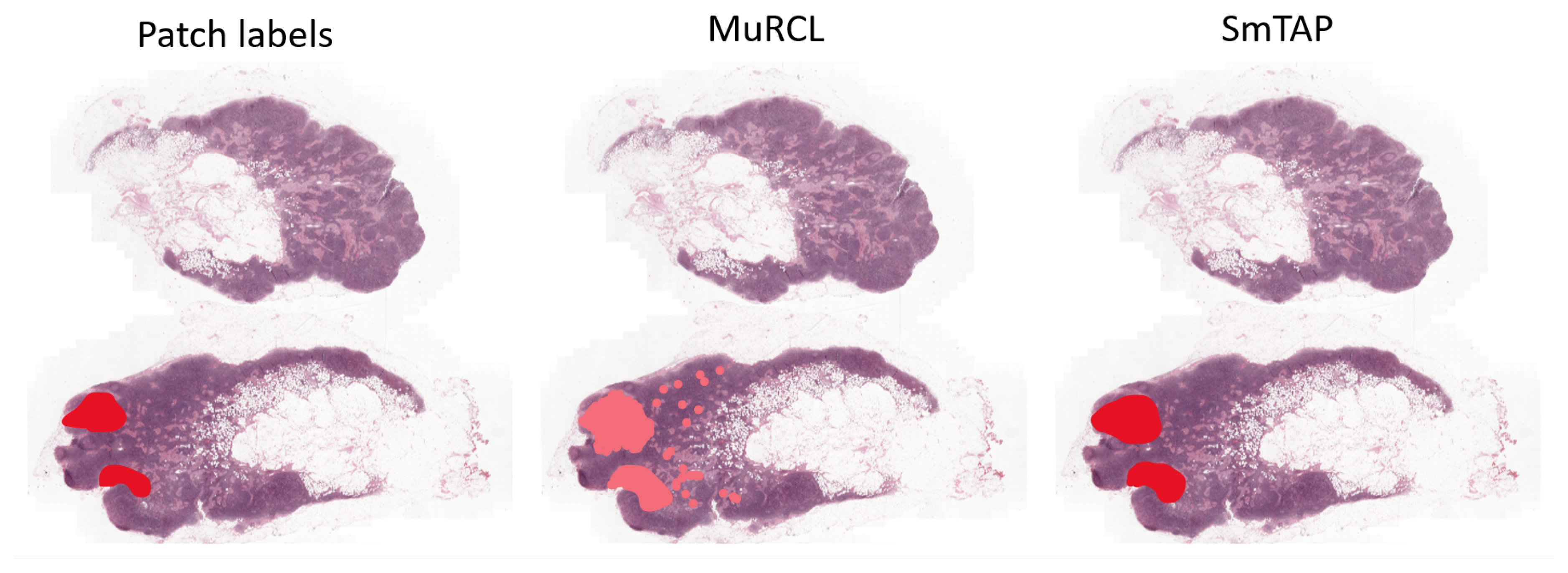

Table A1.
WSI patching configuration and parameters.
| Parameter | Value/Description |
|---|---|
| Input Data | |
| WSI Format | .tif (CAMELYON16) |
| Patch Extraction | |
| Patch Size | pixels |
| Magnification | (target) |
| Scale Factor | 32 (for tissue detection) |
| Tissue Threshold | 0.35 (35% minimum tissue content) |
| Filtering Method | RGB-based tissue detection |
Table A2.
Feature extraction configuration and parameters.
| Parameter | Value/Description |
|---|---|
| Encoder architectures | |
| Base models | ResNet-18; ResNet-50 |
| Weight options | ImageNet pretrained (default); SimCLR pretrained (c16x20-simclr-resnet18.pth used) |
| Feature dimension | 512 (ResNet-18); 2048 (ResNet-50) |
| Input resolution | |
Table A3.
Clustering and spatial graph construction parameters.
| Parameter | Value/Description |
|---|---|
| K-means clustering | |
| Number of clusters | 10 |
| Random seed | 42 (reproducible results) |
| Feature input | patch features (512 or 2048 dimensions) |
| Output format | cluster labels (integer assignments) |
| Spatial graph construction | |
| Graph type | Radius-based spatial connectivity |
| Adjacency rule | if ; otherwise |
| Distance metric | Euclidean distance in coordinate space |
| Radius calculation | , where |
| Spatial radius ratio | 0.1 (10% of maximum coordinate range) |
| Self-loops | Included (include_self=True) |
| Connectivity mode | Binary (0 or 1) |
| Alternative graph types | |
| KNN graph option | k-nearest neighbors in feature space |
| KNN parameter | (default, adjustable) |
| Feature-based | Uses patch features instead of coordinates |
| No-graph option | adj_mat_type=’none’ (skip graph construction) |
References
- Gadermayr, M.; Tschuchnig, M. Multiple instance learning for digital pathology: A review of the state-of-the-art, limitations and future potential. Computerized Medical Imaging and Graphics 2024. [Google Scholar] [CrossRef]
- Litjens, G.; Kooi, T.; Ehteshami Bejnordi, B.; Setio, A.A.A.; Ciompi, F.; Ghafoorian, M.; van der Laak, J.A.W.M.; van Ginneken, B.; Sanchez, C.I. A survey on deep learning in medical image analysis. Medical Image Analysis 2017, 42, 60–88. [Google Scholar] [CrossRef] [PubMed]
- Carbonneau, M.A.; Cheplygina, V.; Granger, E.; Gagnon, G. Multiple instance learning: A survey of problem characteristics and applications. Pattern Recognition 2018. [Google Scholar] [CrossRef]
- Ilse, M.; Tomczak, J.M.; Welling, M. Attention-based deep multiple instance learning. In Proceedings of the Proceedings of the International Conference on Machine Learning; 2018. [Google Scholar]
- Zheng, T.; Jiang, K.; Yao, H. Dynamic policy-driven adaptive multiple instance learning for whole slide image classification. In Proceedings of the Proceedings of the IEEE/CVF Conference on Computer Vision and Pattern Recognition; 2024. [Google Scholar]
- Castro-Macias, F.M.; Morales-Alvarez, P.; Wu, Y.; Molina, R.; Katsaggelos, A.K. Sm: Enhanced localization in Multiple Instance Learning for medical imaging classification. arXiv 2024, arXiv:2410.03276. [Google Scholar] [CrossRef]
- Pereira, R.; Verdelho, M.R.; Barata, C.; Santiago, C. The role of graph-based MIL and interventional training in the generalization of WSI classifiers. arXiv 2025, arXiv:2501.19048. [Google Scholar] [CrossRef]
- Bulten, W.; Balkenhol, M.; Awoumou Belinga, J.J.; Brilhante, A.; Cakir, A.; Farre, X.; Geronatsiou, K.; Molinie, V.; Pereira, G.; Roy, P.; et al. Artificial Intelligence Assistance Significantly Improves Gleason Grading of Prostate Biopsies by Pathologists. arXiv 2020, arXiv:2002.04500. [Google Scholar] [CrossRef]
- Steiner, D.F.; et al. Evaluation of the Use of Combined Artificial Intelligence and Pathologist Assessment to Review and Grade Prostate Biopsies. JAMA Network Open 2020, 3, e2023267. [Google Scholar] [CrossRef]
- Lu, M.Y.; Chen, R.J.; Wang, J.; Dillon, D.; Mahmood, F. Semi-supervised histology classification using deep multiple instance learning and contrastive predictive coding. arXiv 2019, arXiv:1910.10825. [Google Scholar] [CrossRef]
- Dehaene, O.; Camara, A.; Moindrot, O.; de Lavergne, A.; Courtiol, P. Self-supervision closes the gap between weak and strong supervision in histology. arXiv 2020, arXiv:2012.03583. [Google Scholar] [CrossRef]
- Zhu, Z.; Yu, L.; Wu, W.; Yu, R.; Zhang, D. MuRCL: Multi-instance reinforcement contrastive learning for whole slide image classification. IEEE Transactions on Medical Imaging 2022. Early Access. [Google Scholar] [CrossRef]
- Song, A.H.; Jaume, G.; Williamson, D.F.K.; Lu, M.Y.; Vaidya, A.; Miller, T.R.; Mahmood, F. Artificial intelligence for digital and computational pathology. arXiv 2023, arXiv:2401.06148. [Google Scholar] [CrossRef]
- Wang, J.; Mao, Y.; Guan, N.; Xue, C.J. Advances in multiple instance learning for whole slide image analysis. arXiv 2024, arXiv:2408.09476. [Google Scholar] [CrossRef]
- Li, J.; Kuang, H.; Liu, J.; Yue, H.; He, M.; Wang, J. MiCo: Multiple instance learning with context-aware clustering for whole slide image analysis. arXiv 2025, arXiv:2506.18028. [Google Scholar]
- Cersovsky, J.; Mohammadi, S.; Kainmueller, D.; Hoehne, J. Towards hierarchical regional transformer-based multiple instance learning. arXiv 2023, arXiv:2308.12634. [Google Scholar] [CrossRef]
- Wu, S.; Qiu, Y.; Nearchou, I.P.; Prost, S.; Fallowfield, J.A.; Bilen, H.; Kendall, T.J. Multiple instance learning with coarse-to-fine self-distillation. arXiv 2025, arXiv:2502.02707. [Google Scholar]
- Shao, Z.; Bian, H.; Chen, Y.; Wang, Y. TransMIL: Transformer-based correlated multiple instance learning for whole slide image classification. In Proceedings of the Advances in Neural Information Processing Systems; 2021. [Google Scholar]
- Fourkioti, O.; De Vries, M.; Jin, C.; Alexander, D.C.; Bakal, C. CAMIL: Context-aware multiple instance learning for cancer detection and subtyping in whole slide images. arXiv 2023, arXiv:2305.05314. [Google Scholar] [CrossRef]
- Chen, R.J.; Lu, M.Y.; Weng, W.H.; Chen, T.Y. Multimodal co-attention transformer for survival prediction in gigapixel whole slide images. In Proceedings of the Proceedings of the IEEE/CVF International Conference on Computer Vision; 2021. [Google Scholar]
- Chen, R.J.; Chen, C.; Li, Y.; Chen, T.Y. Scaling vision transformers to gigapixel images via hierarchical self-supervised learning. In Proceedings of the Proceedings of the IEEE/CVF Conference on Computer Vision and Pattern Recognition; 2022. [Google Scholar]
- Li, B.; Li, Y.; Eliceiri, K.W. Dual-stream multiple instance learning network for whole slide image classification with self-supervised contrastive learning. In Proceedings of the Proceedings of the IEEE/CVF Conference on Computer Vision and Pattern Recognition; 2021. [Google Scholar]
- Li, X.; Yang, B.; Chen, T.; Lv, S.; Gao, Z.; Li, H. A weakly supervised multiple instance learning based on graph neural network for breast cancer pathology image classification. Proceedings of the International Conference on Communications, Computing and Artificial Intelligence 2023, pp. 47–51. [CrossRef]
- Zhao, B.; Zhang, J.; Ye, D.; Cao, J.; Han, X.; Fu, Q.; Yang, W. RLogist: Fast observation strategy on whole-slide images with deep reinforcement learning. arXiv 2022, arXiv:2212.01737. [Google Scholar] [CrossRef]
- Aliyu, D.A.; Akhir, E.A.P.; Osman, N.A. Optimization techniques in reinforcement learning for healthcare: A review. IEEE Access 2024. In press. [Google Scholar]
- Lakeman, S.; Mohammadi Ziabari, S.; Alsahag, A. A reinforcement-driven multiple instance learning framework for multi-task speaker attribute prediction 2025.
- He, K.; Zhang, X.; Ren, S.; Sun, J. Deep residual learning for image recognition. arXiv 2015, arXiv:1512.03385. [Google Scholar] [CrossRef]
- Chen, T.; Kornblith, S.; Norouzi, M.; Hinton, G. A simple framework for contrastive learning of visual representations. arXiv 2020, arXiv:2002.05709. [Google Scholar] [CrossRef]
- Ehteshami Bejnordi, B.; Veta, M.; Van Diest, P.J.; van Ginneken, B.; et al. Diagnostic assessment of deep learning algorithms for detection of lymph node metastases in women with breast cancer. JAMA 2017. [Google Scholar] [CrossRef]
- Lu, M.Y.; Williamson, D.F.K.; Chen, T.Y.; Chen, R.J.; Barbieri, M.; Mahmood, F. Data efficient and weakly supervised computational pathology on whole slide images. arXiv 2020, arXiv:2004.09666. [Google Scholar] [CrossRef]
- Braakman, N.; Mohammadi Ziabari, S.; Alsahag, A.; Al Husaini, Y. Improving Accuracy and Interpretability in Reinforcement Learning-based Multiple Instance Learning 2026.
- Fu, X.; Meng, X.; Zhou, J.; Ji, Y. High-risk factor prediction in lung cancer using thin CT scans: An attention-enhanced graph convolutional network approach. arXiv 2023, arXiv:2308.14000. [Google Scholar]
- Lu, D.; Kurz, G.; Polomac, N.; Gacheva, I.; Hattingen, E.; Triesch, J. Multiple instance learning for brain tumor detection from magnetic resonance spectroscopy data. arXiv 2021, arXiv:2112.08845. [Google Scholar] [CrossRef]
Figure 1.
High-level overview of the SG-MuRCL framework. A WSI is first converted into a patch-level graph x by a graph-construction module. An RL agent R then draws two stochastic views of that graph, (top branch) and (bottom branch). Each view is passed through a shared GNN-MIL pipeline: a MIL aggregator pools node features into an embedding v, and a projection head converts v into the prediction vector p. The predictions and are compared in the Max-agreement block, which both supplies the contrastive loss for training and produces the scalar reward returned to the RL agent (dashed arrows). The dashed inset (top right) illustrates the agent’s policy over time: Step 0 samples a sub-graph at random; from Step 1 onward the agent follows a learned policy updated at every iteration with the reward produced by the Max-agreement module. This reward-guided sampling steers the agent toward the most discriminative patches while keeping the two branches synchronized through shared weights and a common reward signal.
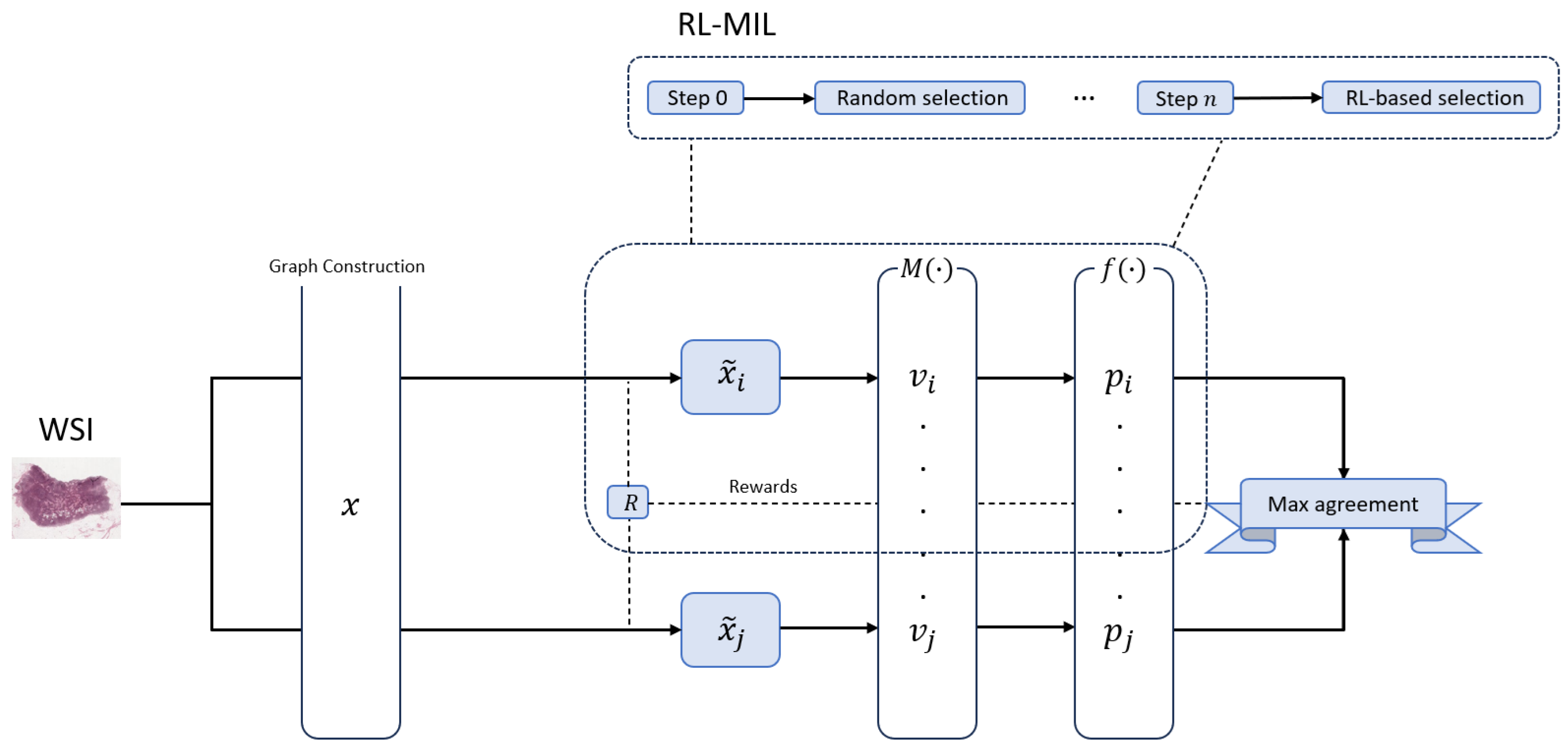
Figure 3.
Patch size distribution in the training and test sets of the CAMELYON16 dataset.
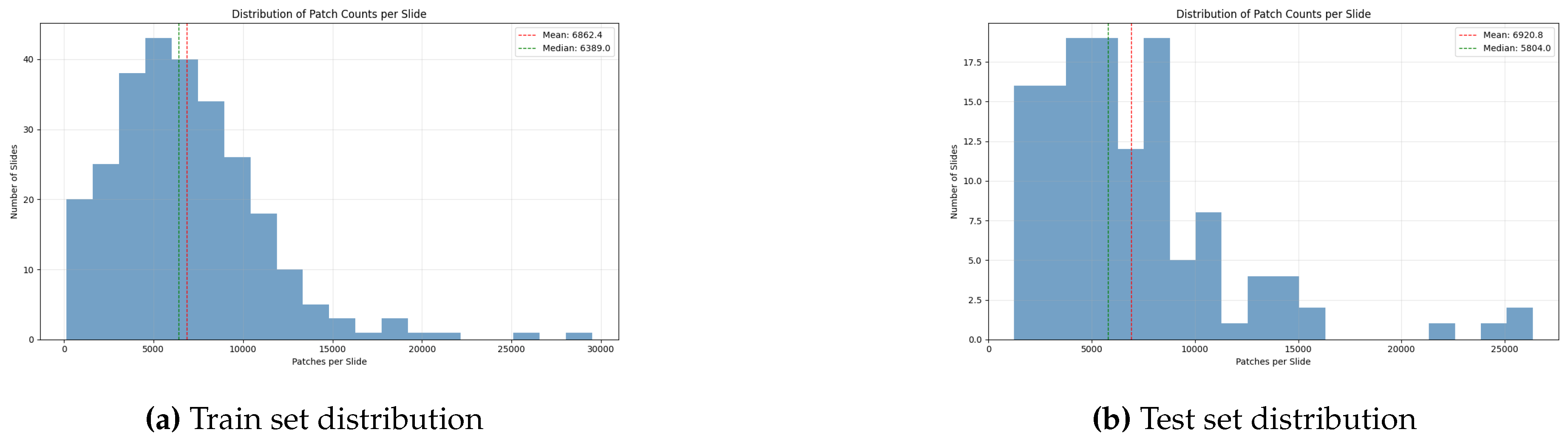
Figure 4.
Learning curves for the three MuRCL baseline configurations on the CAMELYON16 dataset. Each panel shows the training dynamics for its respective backbone.
Figure 4.
Learning curves for the three MuRCL baseline configurations on the CAMELYON16 dataset. Each panel shows the training dynamics for its respective backbone.

Figure 5.
Side-by-side comparison of training loss progression for the stable baseline and the collapsed SG-MuRCL.
Figure 5.
Side-by-side comparison of training loss progression for the stable baseline and the collapsed SG-MuRCL.
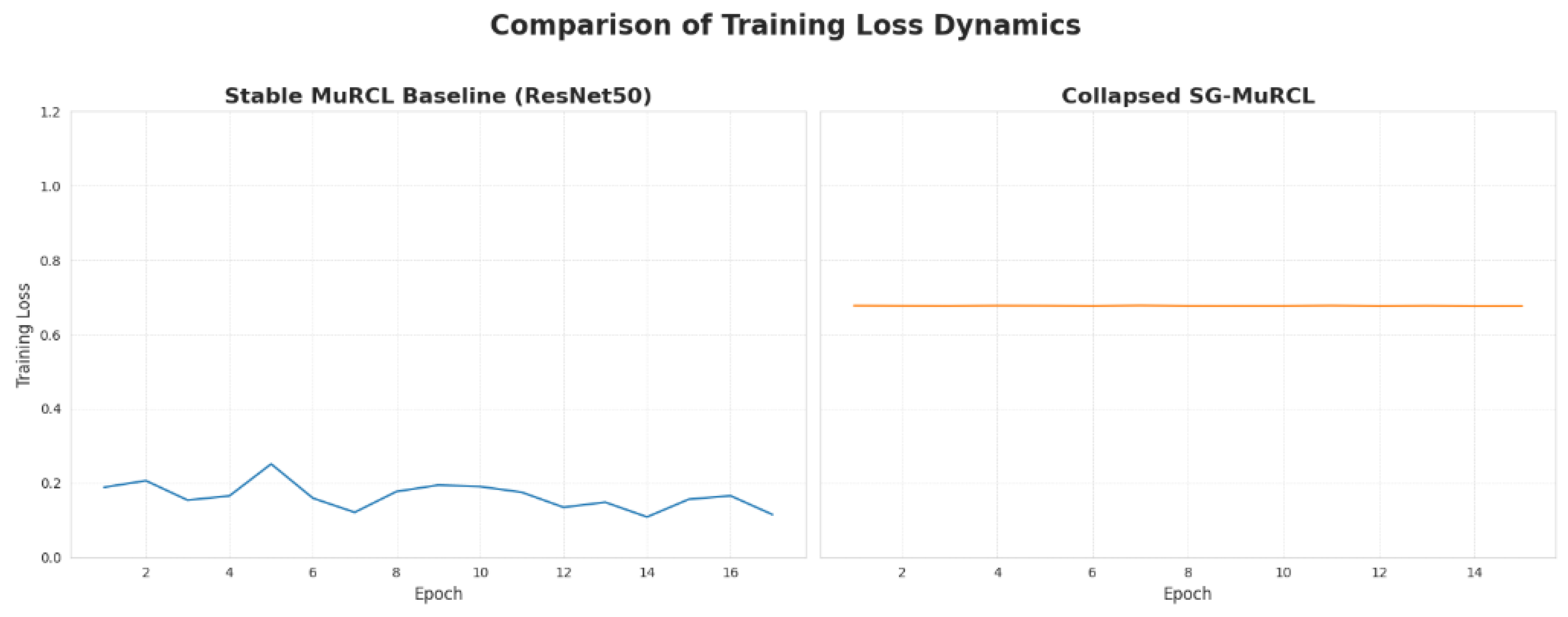
Table 1.
Baseline performance of our MuRCL implementation on the CAMELYON16 test set. The best result in each metric column is highlighted in bold.
Table 1.
Baseline performance of our MuRCL implementation on the CAMELYON16 test set. The best result in each metric column is highlighted in bold.
| Encoder | Loss | Acc. | AUC | Prec. | Recall | F1 |
|---|---|---|---|---|---|---|
| ResNet18 (ImageNet) | 0.645 | 0.744 | 0.652 | 0.750 | 0.490 | 0.593 |
| ResNet18 (SimCLR) | 0.682 | 0.674 | 0.658 | 0.600 | 0.429 | 0.500 |
| ResNet50 (ImageNet) | 0.882 | 0.752 | 0.754 | 0.748 | 0.510 | 0.610 |
Table 2.
Performance of the proposed SG-MuRCL framework on the CAMELYON16 test set for ResNet18, ResNet50 and ResNet18-SimCLR
Table 2.
Performance of the proposed SG-MuRCL framework on the CAMELYON16 test set for ResNet18, ResNet50 and ResNet18-SimCLR
| Encoder | Loss | Acc. | AUC | Prec. | Recall | F1 |
|---|---|---|---|---|---|---|
| SG-MuRCL | 0.912 | 0.620 | 0.500 | 0.000 | 0.000 | 0.000 |
Table 3.
Comparison of estimated average model forward pass latency per WSI.
| Model Configuration | Avg. Inference Time (sec/WSI) |
|---|---|
| MuRCL (Baseline) | ~1.1 |
| SG-MuRCL (Full) | ~3.2 |
Table 4.
Comparison of training loss variance, providing a quantitative measure of stability. A higher variance indicates a successful learning trajectory (decreasing loss), while a very low variance indicates a training collapse into a static, high-loss state.
Table 4.
Comparison of training loss variance, providing a quantitative measure of stability. A higher variance indicates a successful learning trajectory (decreasing loss), while a very low variance indicates a training collapse into a static, high-loss state.
| Model Configuration | Training Loss Variance |
|---|---|
| MuRCL (Stable Baseline) | 0.001279 |
| SG-MuRCL (Collapsed) | 0.000000 |
Disclaimer/Publisher’s Note: The statements, opinions and data contained in all publications are solely those of the individual author(s) and contributor(s) and not of MDPI and/or the editor(s). MDPI and/or the editor(s) disclaim responsibility for any injury to people or property resulting from any ideas, methods, instructions or products referred to in the content. |
© 2025 by the authors. Licensee MDPI, Basel, Switzerland. This article is an open access article distributed under the terms and conditions of the Creative Commons Attribution (CC BY) license (http://creativecommons.org/licenses/by/4.0/).
Copyright: This open access article is published under a Creative Commons CC BY 4.0 license, which permit the free download, distribution, and reuse, provided that the author and preprint are cited in any reuse.


