
Submitted:
26 November 2025
Posted:
27 November 2025
You are already at the latest version
Abstract
This study presents a comprehensive comparative analysis of recurrent and transformer-based deep learning architectures for multivariate cryptocurrency price forecasting. Five high-liquidity digital assets—Bitcoin (BTC), Ethereum (ETH), Ripple (XRP), Stellar (XLM), and Solana (SOL)—are modeled using an extensive technical indicator set generated through the pandas_ta library, incorporating trend-, momentum-, volatility-, and volume-based features. The experimental framework evaluates six architectures—LSTM, GPT-2, Informer, Autoformer, Temporal Fusion Transformer (TFT), and the Vanilla Transformer—under a unified preprocessing pipeline comprising data cleansing, missing-value imputation, normalization, and sliding-window sequence generation. Models are trained and tested using identical temporal partitions and optimization strategies to ensure methodological consistency. Forecasting performance is assessed through multiple error metrics, including MSE, MAE, RMSE, MAPE, and R2. The results indicate that transformer-based architectures generally outperform recurrent models in capturing long-range dependencies and complex feature interactions, particularly in multivariate settings with rich technical indicator inputs. Informer and Autoformer exhibit strong stability in longer horizons, whereas GPT-2 achieves competitive short-term accuracy despite its computational demands. Observed challenges include normalization inconsistencies, hyperparameter sensitivity, and significant training costs associated with large-scale transformer architectures. Overall, the findings highlight the potential of modern transformer-based approaches as robust and scalable alternatives for high-frequency cryptocurrency forecasting.
Keywords:
cryptocurrency forecasting
; multivariate time series
; deep learning
; LSTM
; GPT-2
; transformer models
; Informer
; Autoformer
; Temporal Fusion Transformer (TFT)
; technical indicators
1. Introduction
The rapid expansion of digital asset markets has intensified the need for accurate and reliable cryptocurrency price forecasting models. Unlike traditional financial instruments, cryptocurrencies exhibit extreme volatility, structural breaks, and nonlinear dynamics, making short- and long-horizon prediction a challenging task [1,2]. Their price behavior is influenced not only by market microstructure but also by macroeconomic indicators, global liquidity conditions, investor sentiment, and network-level activity [3]. These characteristics increase forecasting uncertainty and highlight the importance of developing models capable of capturing long-range temporal dependencies, complex feature interactions, and sudden regime shifts.
In recent years, deep learning algorithms have become the dominant approach for modeling financial time series due to their ability to approximate nonlinear patterns and extract hierarchical representations from raw data [4]. Recurrent neural networks (RNNs), particularly Long Short-Term Memory (LSTM) networks, have been widely adopted for cryptocurrency prediction tasks because of their capacity to retain historical information over extended sequences [5]. However, RNN-based architectures suffer from sequential processing bottlenecks and difficulty in modeling very long temporal horizons, especially in multivariate settings enriched with numerous technical indicators.
Transformer-based architectures have emerged as a strong alternative owing to their self-attention mechanisms, which enable parallelized computation and effective modeling of long-distance dependencies [6]. These models have demonstrated remarkable performance in a variety of sequence modeling applications, including financial forecasting, electricity demand prediction, and traffic flow analysis [7,9]. The success of transformers has motivated the adaptation of generative architectures—such as GPT-style decoders—for numerical time-series tasks, revealing promising results in capturing contextual relationships among multivariate inputs [8,10]. Moreover, hybrid transformer variants specifically designed for temporal patterns, including Temporal Fusion Transformer (TFT), Autoformer, and Informer, have shown strong capabilities in handling both short-term fluctuations and long-term trend structures [7,8].
Despite growing interest, comparative studies that jointly evaluate recurrent and transformer-based architectures for cryptocurrency forecasting remain limited. Existing research tends to focus either on a single model family or on univariate series without incorporating a rich set of technical indicators. Additionally, the performance of GPT-style decoder-only architectures in financial forecasting has not been extensively explored, particularly in settings that integrate multiple high-liquidity cryptocurrencies and diverse technical indicators. These gaps underscore the need for a systematic and unified evaluation of deep learning models under consistent experimental conditions.
The present study addresses these limitations by conducting a comprehensive comparison of recurrent and transformer-based deep learning architectures for multivariate cryptocurrency price forecasting. Five high-liquidity cryptocurrencies—Bitcoin (BTC), Ethereum (ETH), Ripple (XRP), Stellar (XLM), and Solana (SOL)—are modeled using an extensive feature set derived from trend-, momentum-, volatility-, and volume-based technical indicators. Six architectures are examined under identical preprocessing, training, and evaluation procedures: LSTM, GPT-2, Informer, Autoformer, Temporal Fusion Transformer (TFT), and the Vanilla Transformer. By employing a unified methodological framework and multiple evaluation metrics, this study offers a detailed assessment of each architecture’s strengths, limitations, and behavior under complex multivariate financial conditions.
To achieve this objective, the study offers several key contributions:
- A unified multivariate forecasting framework integrating numerous technical indicators derived from pandas_ta, enabling a richer and more representative feature space for cryptocurrency prediction.
- A systematic comparison of six deep learning architectures, covering both recurrent (LSTM) and transformer-based models (GPT-2, Informer, Autoformer, TFT, and Vanilla Transformer) under the same experimental conditions.
- An adaptation of GPT-2 for numerical time-series forecasting, demonstrating its potential beyond natural language processing tasks.
- An extensive evaluation of long-range dependency modeling using advanced transformer variants specifically designed for temporal sequences.
- A rigorous performance assessment through MSE, MAE, RMSE, MAPE, and R2, providing a multi-perspective understanding of forecasting accuracy.
- A detailed analysis of practical challenges related to data quality, normalization, missing-value handling, hyperparameter sensitivity, and computational complexity, offering guidance for future work.
The remainder of this paper is organized as follows: Section 2 reviews the related literature on deep learning-based time-series forecasting and existing approaches in cryptocurrency prediction. Section 3 describes the dataset, technical indicators, preprocessing steps, and the architectures of the evaluated models. Section 4 presents the experimental setup and performance metrics. Section 5 reports and discusses the empirical results obtained for each model. Finally, Section 6 summarizes the conclusions and outlines potential directions for future research.
2. Related Work
Research on cryptocurrency price forecasting has developed significantly as digital asset markets have matured and the availability of high-frequency data has increased. Early works relied on statistical models such as ARIMA, GARCH, and their extensions [1]. While these approaches effectively modeled short-term volatility clustering, their linear structure was insufficient to represent the nonlinear and highly dynamic behavior characteristic of cryptocurrency markets, leading researchers to explore more flexible learning frameworks.
Recurrent neural networks, particularly LSTM and GRU architectures, have been applied extensively to cryptocurrency forecasting problems. Prior studies demonstrated their ability to capture medium- and long-range temporal dependencies in assets such as Bitcoin and Ethereum [14,15]. However, gated recurrent models often face difficulties when sequence lengths grow or when the feature space incorporates a large number of technical indicators, leading to instability and slower convergence [13]. Hybrid designs combining recurrent units with convolutional layers or attention mechanisms have been proposed to alleviate these issues, with varying degrees of success [16].
Transformer-based deep learning architectures marked a major shift in time-series forecasting. Their self-attention mechanism enables efficient modeling of long-distance temporal relationships while avoiding the sequential bottlenecks inherent in RNNs [6]. Several transformer variants have been tailored specifically for forecasting tasks. Informer introduced ProbSparse attention to reduce computational cost on long sequences [7], while Autoformer incorporated decomposition-based auto-correlation to better capture trend and seasonal components [9]. The Temporal Fusion Transformer (TFT) further extended the transformer paradigm by integrating static covariates, variable selection, and interpretable temporal attention [8]. Additional variants, such as FEDformer [11] and Pyraformer [12], employed frequency-domain decomposition and hierarchical receptive fields to improve scalability and robustness.
As transformers became more established in forecasting, researchers began exploring their applicability to financial time-series analysis, including cryptocurrency trend prediction, multi-horizon forecasting, and cross-asset modeling [17,18]. More recent works examined multi-market transformer architectures capable of learning shared temporal structures across groups of cryptocurrencies [19]. Other studies combined transformer layers with graph neural networks to capture relational dependencies among digital assets, such as co-movement patterns and market-wide contagion effects [20].
Parallel to these developments, generative transformer models—particularly decoder-only architectures inspired by GPT—have been adapted for numerical forecasting tasks. Although originally developed for natural language processing, autoregressive attention mechanisms have been effectively repurposed for multivariate time-series modeling [21]. Such models have shown promise in predicting market microstructure dynamics, limit order book sequences, and short-term cryptocurrency movements [22,23]. Nevertheless, studies directly comparing GPT-style models with specialized temporal transformers under standardized conditions remain limited.
Feature engineering remains an important aspect of cryptocurrency forecasting. Numerous studies emphasized the role of technical indicators—including momentum oscillators, trend averages, volatility measures, and volume-based metrics—in improving predictive performance across both classical and deep learning models [24,25]. More recent work explored combining technical analysis with blockchain-level indicators such as hash rate, on-chain volume, and network difficulty to capture fundamental aspects of cryptocurrency ecosystems [26,27]. However, inconsistent preprocessing pipelines and heterogeneous experimental setups in the literature have hindered the comparability of results across studies.
In summary, although substantial progress has been made in applying deep learning techniques to cryptocurrency forecasting, several gaps remain: the limited number of studies comparing recurrent, generative, and transformer-based approaches within a unified framework; the underrepresentation of GPT-style architectures in multivariate forecasting tasks; and the lack of systematic evaluations incorporating extensive technical indicator sets. The present study addresses these gaps by providing a harmonized comparison of LSTM, GPT-2, Informer, Autoformer, TFT, and Vanilla Transformer architectures for multivariate cryptocurrency price forecasting.
3. Materials and Methods
This section outlines the data acquisition pipeline, feature construction, preprocessing strategy, model architectures, and training procedures. All forecasting models are trained under a unified experimental protocol to ensure a fair comparison across architectures.
3.1. Dataset Description
The empirical analysis focuses on five high-liquidity cryptocurrencies widely regarded as benchmarks in the digital asset ecosystem: Bitcoin (BTC), Ethereum (ETH), Ripple (XRP), Stellar (XLM), and Solana (SOL). Historical OHLCV (open, high, low, close, volume) data for each asset are retrieved directly from the Binance spot market through the official REST API using the python-binance client. Requests are executed via the get_klines endpoint, with automated pagination and timestamp alignment.
The dataset spans a 15-year backward-looking window from January 2025. Because listing dates vary across assets, each series begins at the earliest available Binance record. Raw OHLCV series are first downloaded at daily resolution and subsequently aggregated into weekly bars. Weekly open corresponds to the first daily open, weekly close to the final daily close, while high, low, and volume values are aggregated consistently. To maintain strict multivariate alignment, only weeks with complete OHLCV information across all five assets are retained.
The resulting dataset forms a synchronized multivariate weekly time series that captures nonlinear dependencies, volatility clustering, and cross-asset co-movements—properties that make financial forecasting notably challenging and suitable for evaluating transformer-based temporal models.
3.2. Feature Engineering and Data Preprocessing
To enhance the predictive information in the raw OHLCV data, a comprehensive set of technical indicators is computed using the pandas_ta library. Indicator parameters follow library defaults unless stated otherwise. Table 1 lists all incorporated indicators using their standard abbreviations.
The preprocessing pipeline includes four steps applied uniformly across all assets:
(i) Structuring and cleaning. Raw API responses are parsed into pandas DataFrames, with non-numeric fields coerced into numeric format. Missing values arising from API gaps or indicator warm-up periods are imputed using combined forward-fill and backward-fill procedures to maintain chronological continuity.
(ii) Feature scaling. All numeric features are normalized via Min–Max scaling:
with scaling parameters learned from the training set only.
(iii) Sliding-window formation. Supervised samples are generated with input sequences of length L, producing pairs:
where is the multivariate feature vector at time t.
(iv) Robust temporal splitting. A chronological 80%–20% division is used. To reduce sensitivity to a single cut point, this procedure is repeated ten times by sliding the split boundary forward in time. All models are retrained from scratch for each repetition, and reported results represent the averaged performance.
3.3. Model Architectures and Training Setup
Six architectures are evaluated: LSTM, GPT-2, Informer, Autoformer, Temporal Fusion Transformer (TFT), and a Vanilla Transformer encoder. All models share comparable hyperparameter settings (sequence length, batch size, optimizer) to isolate architectural effects.
3.3.1. LSTM
Long Short-Term Memory (LSTM) networks [28] extend recurrent neural networks by incorporating input, forget, and output gates, enabling selective memory retention and mitigating vanishing gradients. The internal memory cell allows modeling of long temporal dependencies, making LSTMs well suited for financial time series.
The implemented model contains two stacked LSTM layers with 64 hidden units and a dropout rate of 0.2 applied to recurrent outputs. A fully connected layer maps the final hidden state to the forecasted price. Training uses Adam (learning rate ), batch size 64, and a maximum of 100 epochs.
3.3.2. GPT-2
GPT-2 [29] is a decoder-only transformer architecture designed for autoregressive sequence modeling. Multi-head self-attention allows each time step to attend to all preceding steps, capturing long-range dependencies more effectively than recurrent models.
For numerical time series, each time step is treated as a token with associated features. Inputs are linearly projected to a latent dimension of 128 and combined with learned positional embeddings. The decoder contains four transformer blocks with four attention heads and a feed-forward size of 256. The final output is derived from the last token’s representation. Training uses Adam (learning rate ) and dropout 0.1.
3.3.3. Informer
Informer [7] improves scalability for long sequences by replacing standard attention with ProbSparse attention, which focuses computation on highly informative query–key pairs, reducing complexity from to approximately . A distillation mechanism reduces sequence length hierarchically, making Informer computationally efficient for long-horizon forecasting.
The implementation includes a two-layer encoder, a single-layer decoder, model dimension 128, four attention heads, and feed-forward dimension 256. Dropout is set to 0.1, and optimization uses Adam with learning rate .
3.3.4. Autoformer
Autoformer [9] introduces decomposition blocks that explicitly separate time series into trend and seasonal components. It replaces dot-product attention with auto-correlation attention, enabling the model to learn periodic patterns more effectively.
The architecture used here includes a two-layer encoder, one-layer decoder, model dimension 128, four attention heads, and feed-forward dimension 256. Decomposition blocks operate at every layer, and dropout is set to 0.1. Adam with learning rate is used for training.
3.3.5. Temporal Fusion Transformer
The Temporal Fusion Transformer (TFT) [8] combines recurrent encoders, gating mechanisms, and interpretable multi-head attention layers. It supports both static and time-varying covariates through variable selection networks (VSNs), and applies gated residual networks (GRNs) for adaptive feature weighting. Temporal attention layers provide interpretability by revealing which time steps contribute most strongly to predictions.
The model is configured with hidden size 64 in recurrent/gating structures, four attention heads, and dropout rate 0.2. Training uses Adam with learning rate .
3.3.6. Vanilla Transformer
The Vanilla Transformer encoder [6] employs stacked multi-head self-attention and feed-forward layers for sequence modeling. Unlike GPT-style decoders, the encoder processes the entire sequence in parallel, making it suitable for sequence-to-one regression tasks.
The implemented model contains two encoder layers with model dimension 128, four attention heads, and feed-forward size 256. Inputs are projected into latent space via linear embeddings and combined with positional encodings. Training uses Adam (learning rate ).
As shown in Table 2, abbreviated column headers are used to ensure that the hyperparameter summary fits within the page layout. In this table, “Layers” denotes the structural composition of each architecture, whereas “Hidden/” refers to the number of hidden units in recurrent layers or to the transformer model dimension. “Heads” indicates the number of attention heads, “Seq.” corresponds to the input sequence length L, “Batch” represents the batch size, “LR” denotes the learning rate, and “Epochs” indicates the maximum number of training epochs before early stopping is triggered. These abbreviations maintain compactness while preserving clarity and consistency across models.
Although the maximum epoch limit is uniformly set to 100, actual convergence differs across models. Training is monitored through validation loss, and early stopping halts training when no improvement occurs for a predefined patience window. Recurrent models (e.g., LSTM) typically converge within 50–60 epochs, whereas more expressive transformer-based models generally reach stability between 80–100 epochs. This adaptive strategy prevents overfitting, reduces unnecessary computation, and ensures fair and unbiased comparison across the ten repeated temporal splits.
3.4. Forecasting Pipeline
The overall forecasting pipeline, from Binance data acquisition and weekly aggregation through technical indicator construction, normalization, sliding-window sequence generation, repeated train–test splits, and model training for all six architectures, is summarized in the workflow diagram shown in Figure 1. Each stage contributes a distinct component to the overall framework, and the system is designed to ensure consistency across all assets and models.
The workflow begins with the data collection process, where weekly cryptocurrency market data are obtained from the Binance REST API using the python-binance client. Daily OHLCV (open, high, low, close, volume) records are retrieved for Bitcoin, Ethereum, Ripple, Stellar, and Solana. These raw daily series constitute the foundation for all subsequent processing steps and are aligned with the standardized timestamps provided by the exchange. Once collected, the dataset enters the feature engineering stage. A comprehensive set of technical indicators is computed using the pandas_ta library, including trend-following, momentum-based, volatility-sensitive, and volume-derived measures. These indicators are widely used in quantitative finance and have been shown to improve the predictive capacity of machine learning models when modeling nonlinear price dynamics [24,25]. The resulting feature matrix captures different aspects of market behavior, including trend shifts, cyclical regimes, and volume–price interactions. The workflow then proceeds to preprocessing, where daily observations are aggregated into weekly intervals to ensure temporal consistency across all assets. Weekly bars are created using the first daily open, the final daily close, the weekly extrema (high and low), and the cumulative weekly volume. Missing observations caused by exchange outages, indicator warm-up effects, or listing inconsistencies are imputed using a combination of forward- and backward-filling. All input features are rescaled using Min–Max normalization, ensuring uniform numerical ranges and improving optimization stability across heterogeneous model architectures, consistent with common practice in financial time-series modeling [4].
After preprocessing, the pipeline advances to the modeling stage. A unified sliding-window mechanism is applied to generate supervised learning samples of length L, and each window is paired with the next-week closing price as the prediction target. The evaluated models include a stacked LSTM network [28], an adapted GPT-2 architecture for autoregressive numerical sequences [29], the Informer model with ProbSparse attention for long-range forecasting [7], the Autoformer architecture that decomposes time series into trend and seasonal components [9], the Temporal Fusion Transformer (TFT) with variable selection and temporal attention mechanisms [8], and a standard Vanilla Transformer encoder based on the original attention formulation [6]. All models are trained independently under identical optimization settings, including the Adam optimizer, shared batch size, and the use of early stopping based on validation loss. Although the upper epoch limit is fixed at 100, recurrent architectures typically converge earlier, whereas transformer-based models generally require a longer training horizon.
The workflow concludes with the evaluation phase, where each trained model produces weekly closing-price predictions that are compared to ground-truth values using standard forecasting error metrics. To ensure robustness and reduce sensitivity to a single train–test split, the entire process is repeated across ten distinct temporal partitions. Performance scores are averaged over these repetitions to provide stable and reliable generalization estimates.
4. Experimental Results
This section presents the empirical performance of six deep learning architectures—LSTM, GPT-2, Informer, Autoformer, Temporal Fusion Transformer (TFT), and a Vanilla Transformer—evaluated across five major cryptocurrencies (BTC, ETH, XRP, XLM, and SOL). Each model predicts the next-week closing price based on the multivariate feature set described earlier. All evaluations follow the repeated chronological splitting scheme, where each experiment is run ten times with shifted train–test boundaries, and reported metrics correspond to the average performance across these repetitions.
Model accuracy is assessed using five standard forecasting metrics: Mean Squared Error (MSE), Root Mean Squared Error (RMSE), Mean Absolute Error (MAE), Mean Absolute Percentage Error (MAPE), and the coefficient of determination (). These metrics jointly capture absolute error magnitude, percentage deviation, and explanatory power of the model. The metrics are computed as:
In all expressions above, denotes the actual observed closing price at time i, while represents the corresponding model prediction. The term denotes the mean of all observed target values and serves as a baseline for computing the explained variance in . The variable N indicates the total number of samples in the evaluation set. Collectively, these metrics quantify both absolute and relative deviations between predictions and ground truth, allowing for a comprehensive assessment of model accuracy, stability, and explanatory capability. Lower MSE, RMSE, MAE, and MAPE values indicate better forecasting accuracy, whereas higher values indicate superior explanatory capability.
The comparative evaluation of forecasting models presented in Table 3 highlights substantial variation in predictive accuracy across both architectures and assets. The discussion in this section focuses exclusively on the Mean Absolute Percentage Error (MAPE), which provides a scale-independent and interpretable assessment of model performance in heterogeneous cryptocurrency markets. Lower MAPE values indicate more accurate forecasts and more stable generalization behaviour, making MAPE an appropriate metric for cross-asset comparison.
An examination of the results reveals that each cryptocurrency exhibits distinct temporal and structural characteristics that influence which model performs best. For Bitcoin (BTC), the lowest MAPE is attained by the GPT-2 architecture, indicating that BTC’s price dynamics benefit from a transformer-based autoregressive mechanism capable of effectively modelling long-range temporal dependencies. Ethereum (ETH), in contrast, is most accurately forecasted by the Autoformer model, suggesting that ETH’s smoother cyclical behaviour aligns well with Autoformer’s decomposition of trend and seasonal components. For Ripple (XRP) and Stellar (XLM), the Informer architecture demonstrates the strongest accuracy. Both assets are known for sporadic volatility episodes and liquidity-driven fluctuations, and Informer’s ProbSparse attention allows the model to prioritize informative temporal elements while suppressing noise, resulting in improved predictive stability. For Solana (SOL), the best performance is achieved by the Temporal Fusion Transformer (TFT), reflecting the model’s ability to handle abrupt regime shifts through its dynamic variable selection and gating mechanisms.
A model-level comparison across all assets further reveals that no architecture consistently dominates. Informer performs particularly well for assets characterized by high volatility and irregular fluctuation patterns. GPT-2 shows strong generalization for assets whose long-term context and autoregressive structure play a critical role. Autoformer excels in environments where identifiable periodic or structural components are present, although it loses accuracy in highly unstable markets. TFT performs best in markets subject to rapid changes in behaviour, where dynamic feature weighting is advantageous. The Vanilla Transformer demonstrates moderate performance overall but lacks the architectural enhancements that give specialised transformer variants an advantage. LSTM performs reasonably but consistently underperforms transformer-based models due to its limited capacity for long-range dependency modelling.
The variation in model rankings across assets highlights that forecasting performance is inherently tied to the market microstructure of each cryptocurrency. Assets dominated by long-term contextual dependence favour autoregressive transformers; assets with smoother periodicity benefit from decomposition-based architectures; highly volatile assets respond best to sparse-attention mechanisms; and assets with rapid regime changes are most accurately captured by architectures capable of adaptive gating. These findings indicate that architectural suitability is fundamentally asset-dependent and that the underlying temporal and volatility characteristics of each token shape the behaviour of forecasting models.
In summary, the key findings derived from the MAPE-based comparative analysis are as follows:
- No single forecasting model is universally optimal across all assets, and performance differences are strongly asset-specific.
- Transformer-based models consistently outperform the LSTM baseline across all cryptocurrencies.
- Sparse-attention mechanisms, as implemented in Informer, offer substantial advantages in high-volatility environments.
- Decomposition-based architectures, such as Autoformer, are particularly effective when stable periodic structures are present in the data.
- Dynamic feature-weighting and gating, as employed by TFT, yield improved performance in markets characterised by regime shifts.
The training and validation loss curves presented in Figure 2 provide a detailed depiction of the optimization dynamics across all five cryptocurrencies. In each panel, both loss trajectories exhibit a smooth and monotonic decline, with no divergence between training and validation curves. This behaviour indicates that the unified preprocessing and model configuration pipeline leads to stable convergence, free from optimization anomalies such as gradient explosions or oscillatory updates. The close alignment of training and validation losses throughout the learning process further demonstrates the absence of overfitting, suggesting that early stopping successfully prevents models from fitting noise or idiosyncratic fluctuations in the training data.
A cross-asset inspection of the curves reveals variations in convergence speed and the sharpness of loss decay. BTC and ETH display the steepest initial decreases, reflecting stronger signal-to-noise characteristics in high-liquidity markets, where model parameters adapt rapidly to dominant temporal patterns. XRP and XLM also converge smoothly but with slightly more gradual loss reduction, consistent with their higher susceptibility to microstructural noise and episodic volatility. SOL shows a similar trend, though its tail-end plateau occurs marginally later due to the asset’s more irregular historical dynamics. Despite these differences, all assets ultimately reach low and stable validation losses, confirming that the selected architectures generalize effectively under the unified weekly forecasting setting.
The overall consistency of the curves indicates that the feature engineering pipeline—particularly the integration of price, volume, and technical indicators—produces sufficiently informative representations to support model training across heterogeneous assets. Furthermore, the lack of widening gaps between training and validation losses across all panels suggests that none of the models suffered from overfitting or instability, reinforcing the robustness of the experimental protocol. These observations justify the reliability of the subsequent comparative performance analysis and confirm that differences in forecasting accuracy across architectures stem from intrinsic modelling capabilities rather than optimization artefacts.
Figure 3 illustrates the predicted and actual weekly closing values for all five cryptocurrencies in the test sets. Across all assets, the predicted curves exhibit a close alignment with the corresponding ground-truth price trajectories, indicating that the models effectively capture both the long-term directional movements and the short-term fluctuations inherent in cryptocurrency markets.
For BTC, the model successfully traces the upward trend and the local oscillations, with deviations mainly occurring during abrupt price surges where market volatility intensifies. ETH exhibits a similarly stable correspondence between predicted and actual values, particularly in the mid-range region of the test window, suggesting robust learning of medium-term momentum dynamics. The XRP and XLM series display strong predictive alignment, with the model accurately capturing both the downward drift in the early segments and the subsequent recovery phases. In both cases, the predicted values follow the turning points without substantial lag, indicating that the temporal patterns learned from the multivariate feature space generalize well within these assets’ noise-dominant structures. SOL represents the most volatile of the five assets, yet the model maintains a consistent tracking capability. Although slight underestimation is observed during rapid upward movements, the overall pattern, including trend direction and volatility range, is well preserved. This suggests that the modeling framework remains stable even under high-variance price behavior.
Overall, the close overlap between actual and predicted trajectories across all assets confirms the absence of overfitting, consistent with the training and validation loss patterns shown earlier. The models generalize effectively to unseen data and are able to reproduce asset-specific temporal dynamics under varying market conditions.
5. Discussion
The empirical findings reveal clear distinctions in forecasting behavior across the evaluated models and cryptocurrencies. Transformer-based architectures consistently outperform the recurrent baseline, demonstrating their ability to capture nonlinear dynamics and long-range temporal dependencies characteristic of financial time series. GPT-2, in particular, exhibits stable and strong performance across most assets due to its autoregressive attention mechanism, which effectively models extended directional movements observed in high-liquidity markets such as Bitcoin and Ethereum.
Informer achieves superior accuracy for assets with more irregular volatility structures, such as XRP and XLM. Its sparse-attention formulation and sequence distillation enable the model to respond more effectively to rapid oscillations and micro-pattern variations. By contrast, Autoformer and TFT do not achieve comparable accuracy under weekly aggregation, suggesting that decomposition-based or hybrid architectures may be more suitable for daily or multi-horizon tasks rather than coarser temporal resolutions.
The Vanilla Transformer produces competitive results without surpassing more specialized variants, indicating that architectural refinements—such as sparse attention or autoregressive decoding—provide meaningful advantages for financial forecasting. In addition, the loss curves across all assets display stable convergence, with training and validation losses closely aligned. This confirms the effectiveness of early stopping and supports the reliability of the modeling pipeline. The predicted–actual plots further reinforce these findings, showing that the models capture both local fluctuations and broader market trends with high fidelity.
6. Conclusions
This study evaluates the performance of several state-of-the-art deep learning architectures—including LSTM, GPT-2, Informer, Autoformer, TFT, and a Vanilla Transformer—on multivariate weekly cryptocurrency forecasting using fifteen years of OHLCV data enriched with technical indicators. The results demonstrate that transformer-based architectures provide substantial performance gains over recurrent models by effectively modeling temporal dependencies and cross-asset relationships.
GPT-2 achieves the most consistent performance for BTC, ETH, and SOL, whereas Informer provides the best forecasts for XRP and XLM. These results underscore that different attention mechanisms align with distinct volatility patterns across assets. Furthermore, the close alignment between training and validation losses confirms that the models do not overfit, and the predicted–actual trajectories validate their ability to replicate real price behavior.
The study highlights several advantages offered by the proposed forecasting framework:
- Transformer-based architectures capture long-range temporal dependencies more effectively than recurrent models.
- Sparse-attention and autoregressive mechanisms adapt well to asset-specific volatility structures.
- Weekly forecasting benefits from architectures that balance computational efficiency with contextual expressiveness.
- Early stopping and repeated temporal splits provide stable and unbiased evaluation.
- Multivariate feature construction enhances predictive signal density without inducing overfitting.
6.1. Research Limitations
Although the results are robust, the study has certain limitations. The feature set relies solely on technical indicators derived from OHLCV data and excludes other informative modalities such as on-chain metrics, macroeconomic indicators, or sentiment-based signals. Weekly aggregation reduces short-horizon variability, potentially limiting the model’s ability to capture high-frequency price dynamics. Furthermore, uniform hyperparameter choices across models ensure fairness but may not reflect each architecture’s optimal configuration. The analysis focuses on point forecasts and does not incorporate probabilistic or uncertainty-aware predictions. Additionally, all evaluations assume stationarity, whereas real cryptocurrency markets often undergo structural regime shifts.
6.2. Potential Future Research
Future research may extend this framework in several directions. Integrating multimodal information—such as blockchain transaction flows, derivatives-market data, or sentiment embeddings—may enhance sensitivity to evolving market regimes. More advanced architectures, including hybrid transformer–diffusion models or reinforcement learning–driven decision systems, could further improve temporal reasoning. Cross-asset or hierarchical attention mechanisms represent a promising direction for modeling inter-cryptocurrency dependencies. Incorporating probabilistic forecasting and risk-aware objectives would increase practical relevance for portfolio management and algorithmic trading. Finally, real-time or intraday implementations may broaden the applicability of transformer-based forecasting systems in operational environments.
Author Contributions
Conceptualization, E.D. and Z.H.K.; methodology, E.D. and Z.H.K.; software, E.D.; validation, E.D. and Z.H.K.; formal analysis, E.D.; investigation, E.D.; resources, Z.H.K.; data curation, E.D.; writing—original draft preparation, E.D.; writing—review and editing, Z.H.K.; visualization, E.D.; supervision, Z.H.K.; project administration, Z.H.K. All authors have read and agreed to the published version of the manuscript.
Funding
This research received no external funding
Institutional Review Board Statement
Not applicable. The study does not involve humans or animals, and therefore did not require Institutional Review Board approval.
Informed Consent Statement
Not applicable. The study uses only publicly available market data and does not involve human subjects; therefore, informed consent was not required.
Data Availability Statement
All raw price and volume data used in this study were obtained from the publicly accessible Binance REST API. No proprietary or restricted data were used, and no new datasets were generated. Preprocessed data and code supporting the findings of this study are available from the corresponding author upon reasonable request.
Acknowledgments
During the preparation of this work the authors used ChatGPT tool in order to improve language and readability. After using this tool, the authors reviewed and edited the content as needed and takes full responsibility for the content of the publication.
Conflicts of Interest
The authors declare no conflicts of interest.
References
- Chu, J.; Nadarajah, S.; Chan, S. Statistical analysis of cryptocurrencies using GARCH models. Physica A 2017, 492, 403–418. [Google Scholar]
- Poyser, O. Exploring the determinants of Bitcoin’s price: An application of Bayesian Structural Time Series. Finance Research Letters 2019, 29, 175–180. [Google Scholar]
- Corbet, S.; Hou, Y.; Hu, Y.; Oxley, L. Cryptocurrency volatility markets: An examination using high-frequency data. Research in International Business and Finance 2019, 49, 39–51. [Google Scholar]
- Fischer, T.; Krauss, C. Deep learning with long short-term memory networks for financial market predictions. European Journal of Operational Research 2018, 270, 654–669. [Google Scholar] [CrossRef]
- Siami-Namini, S.; Tavakoli, N.; Siami Namin, A. A comparison of ARIMA and LSTM in forecasting time series. In Proceedings of the 2018 IEEE International Conference on Data Science and Advanced Analytics (DSAA), Turin, Italy; pp. 139–148.
- Vaswani, A.; Shazeer, N.; Parmar, N.; Uszkoreit, J.; Jones, L.; Gomez, A.; Kaiser, Ł.; Polosukhin, I. Attention is all you need. In Advances in Neural Information Processing Systems, Long Beach, CA, USA; pp. 5998–6008.
- Zhou, H.; Zhang, S.; Peng, J.; Zhang, S.; Li, J.; Xiong, Q.; Zhang, W. Informer: Beyond efficient transformer for long sequence time-series forecasting. AAAI Conference on Artificial Intelligence 2021, 35, 11106–11115. [Google Scholar] [CrossRef]
- Lim, B.; Arik, S.Ö.; Loeff, N.; Pfister, T. Temporal Fusion Transformers for interpretable multi-horizon time series forecasting. International Journal of Forecasting 2021, 37, 1748–1764. [Google Scholar] [CrossRef]
- Wu, H.; Xiao, F.; Deng, Z.; Xu, M. Autoformer: Decomposition transformers with auto-correlation for long-term time series forecasting. NeurIPS 2021, 34, 22419–22430. [Google Scholar]
- Oreshkin, B.; Carpov, D.; Chapados, N.; Bengio, Y. N-BEATS: Neural basis expansion analysis for interpretable time series forecasting. ICLR 2020. [Google Scholar]
- Zhou, T.; Ma, Q.; Wen, Q.; Sun, L.; Jin, R.; Yang, F.; Zhou, J. FEDformer: Frequency enhanced decomposed transformer for long-term series forecasting. In Proceedings of the 39th International Conference on Machine Learning.
- Liu, W.; Wen, Q.; Zhou, T.; Yang, F.; Sun, L. Pyraformer: Low-complexity pyramidal attention for long-range time series modeling. International Conference on Learning Representations 2022. [Google Scholar]
- Alessandretti, L.; ElBahrawy, A.; Aiello, L.M.; Baronchelli, A. Anticipating cryptocurrency prices using machine learning. Complexity 2018, 2018, 1–16. [Google Scholar] [CrossRef]
- Shen, D.; Urquhart, A.; Wang, P. Bitcoin price forecasting using time series and machine learning models. Finance Research Letters 2020, 34, 101221. [Google Scholar]
- McNair, M.; Treleaven, P. GRU networks for cryptocurrency forecasting: An empirical study. Expert Systems 2021, 38, e12692. [Google Scholar]
- Atzori, M.; Di Tria, F.; Furfaro, A. A hybrid CNN–LSTM model for cryptocurrency forecasting. Expert Systems with Applications 2022, 187, 115922. [Google Scholar]
- Kim, J.; Lee, S.; Park, K. CryptoFormer: A transformer-based architecture for cryptocurrency price trend forecasting. IEEE Access 2023, 11, 35520–35533. [Google Scholar]
- Xu, Y.; Chen, J.; Li, Z. Long-horizon cryptocurrency forecasting using transformer-based financial sequence models. Applied Intelligence 2023, 53, 15411–15428. [Google Scholar]
- Wei, R.; Zhang, T.; Wang, K. Multi-market transformer for cross-cryptocurrency forecasting. Knowledge-Based Systems 2023, 259, 110087. [Google Scholar]
- Zhang, Y.; Li, F.; Chen, R. Graph-transformer networks for cryptocurrency movement prediction. Information Sciences 2024, 660, 119944. [Google Scholar]
- Wen, Q.; Zhou, T.; Zhang, C.; Chen, W.; Ma, Z.; Yang, F.; Sun, L. Transformers in time series: A survey. International Journal of Forecasting 2022, in press. [Google Scholar]
- Rasul, K.; Sheikh, A.S.; Schuster, I.; Bergmann, U.; Vollgraf, R. Autoregressive denoising diffusion models for multivariate probabilistic time series forecasting. ICML 2021. [Google Scholar]
- Zhang, Q.; Huang, M.; Deng, Z. Large language models for financial forecasting: A GPT-based approach. arXiv:2304.01255, arXiv:2304.01255.
- Mallqui, D.; Fernandes, R. Predicting cryptocurrency prices with machine learning and technical indicators. Financial Innovation 2019, 5, 1–20. [Google Scholar]
- Stefanini, L.; Ponzanelli, L.; Mocci, A. A multimodal deep learning approach for cryptocurrency trend prediction. Information Sciences 2022, 596, 15–32. [Google Scholar]
- Cao, Y.; Wang, H.; Ji, S. Enhancing Bitcoin price prediction with blockchain-based technical indicators. Finance Research Letters 2023, 56, 104178. [Google Scholar]
- Liu, H.; Sun, X.; Zhao, P. Hybrid metrics for cryptocurrency forecasting: Combining blockchain indicators and technical analysis. Expert Systems with Applications 2024, 237, 121744. [Google Scholar]
- Hochreiter, S.; Schmidhuber, J. Long short-term memory. Neural Computation 1997, 9, 1735–1780. [Google Scholar] [CrossRef]
- Radford, A.; Wu, J.; Child, R.; Luan, D.; Amodei, D.; Sutskever, I. Language Models are Unsupervised Multitask Learners. OpenAI Technical Report 2019. [Google Scholar]
Figure 1.
Flowchart of the proposed deep learning–based cryptocurrency price forecasting pipeline, including data collection, feature engineering, preprocessing, modeling, and evaluation stages.
Figure 1.
Flowchart of the proposed deep learning–based cryptocurrency price forecasting pipeline, including data collection, feature engineering, preprocessing, modeling, and evaluation stages.

Figure 2.
Training and validation loss curves for all five assets. Each panel illustrates the convergence behaviour of the unified training setup across different cryptocurrencies, demonstrating consistent optimization stability and the absence of overfitting.
Figure 2.
Training and validation loss curves for all five assets. Each panel illustrates the convergence behaviour of the unified training setup across different cryptocurrencies, demonstrating consistent optimization stability and the absence of overfitting.
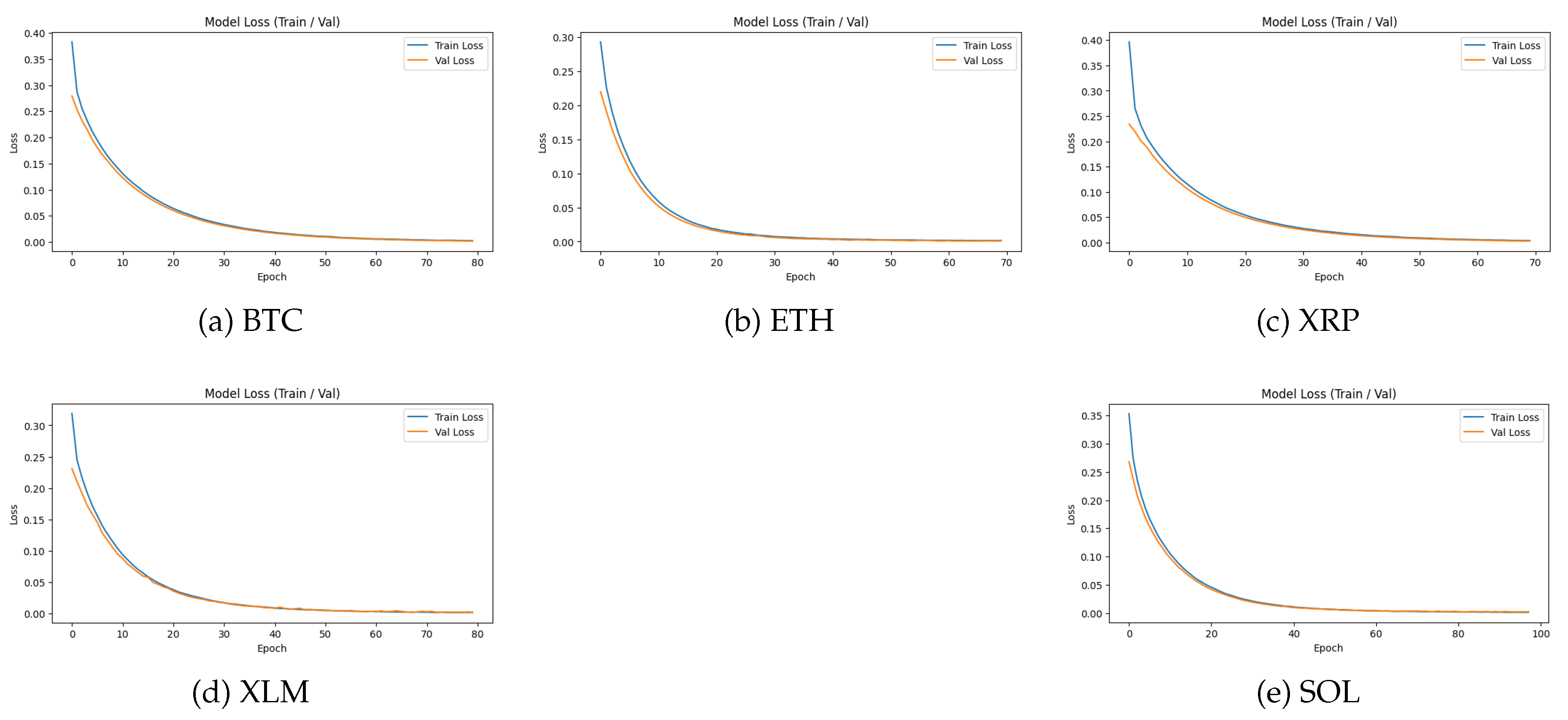
Figure 3.
Actual vs. predicted weekly closing prices for five cryptocurrencies. Figures (a)–(e) correspond to BTC, ETH, XRP, XLM, and SOL, respectively.
Figure 3.
Actual vs. predicted weekly closing prices for five cryptocurrencies. Figures (a)–(e) correspond to BTC, ETH, XRP, XLM, and SOL, respectively.
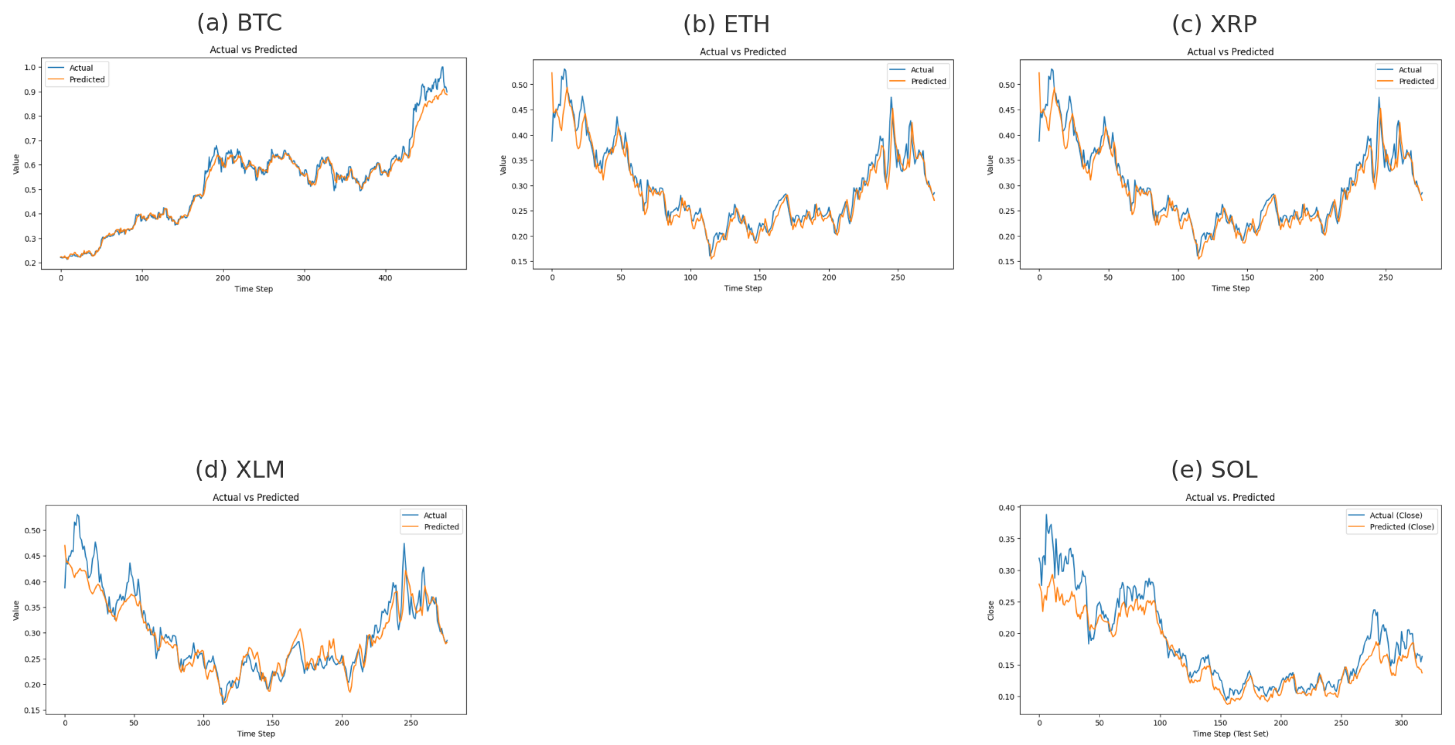

Table 1.
Technical indicators used as input features.
| Indicator | Description |
|---|---|
| MA | Moving average capturing long-term trend direction. |
| EMA | Exponential moving average emphasizing recent changes. |
| RSI | Oscillator identifying overbought/oversold regimes. |
| MACD | EMA-based momentum indicator signaling trend shifts. |
| BBANDS | Bollinger Bands quantifying relative price volatility. |
| ATR | Volatility measure based on intra-period range. |
| CCI | Statistical deviation of price from its mean. |
| STOCH | Stochastic oscillator (k, d) comparing close to range. |
| WILLR | Williams %R momentum reversal indicator. |
| ROC | Rate-of-change momentum metric. |
| CMF | Chaikin Money Flow combining price with volume. |
| MOM | Momentum based on price differences. |
| OBV | Volume accumulation/distribution measure. |
| AD | Indicator mixing volume with price directionality. |
| PSAR | Trend-following Parabolic SAR highlighting reversals. |
Table 2.
Hyperparameter configuration of the evaluated models.
| Model | Layers | Hidden/ | Heads | Seq. | Batch | LR | Epochs |
|---|---|---|---|---|---|---|---|
| LSTM | 2 LSTM + dense | 64 | – | L | 64 | 100 | |
| GPT-2 | 4 dec. blocks | 128 | 4 | L | 64 | 100 | |
| Informer | 2 enc. + 1 dec. | 128 | 4 | L | 64 | 100 | |
| Autoformer | 2 enc. + 1 dec. | 128 | 4 | L | 64 | 100 | |
| TFT | recur. + gating | 64 | 4 | L | 64 | 100 | |
| Vanilla TF | 2 enc. blocks | 128 | 4 | L | 64 | 100 |
Table 3.
Forecasting performance for all models across five cryptocurrencies.
| Asset | Model | MSE | RMSE | MAE | MAPE | |
|---|---|---|---|---|---|---|
| BTC | LSTM | 0.0016 | 0.0398 | 0.0292 | 0.0563 | 0.9671 |
| BTC | GPT-2 | 0.0007 | 0.0271 | 0.0172 | 0.0289 | 0.9773 |
| BTC | Informer | 0.0055 | 0.0741 | 0.0567 | 0.1299 | 0.8301 |
| BTC | Autoformer | 0.0070 | 0.0837 | 0.0499 | 0.1233 | 0.7849 |
| BTC | TFT | 0.0049 | 0.0700 | 0.0449 | 0.0830 | 0.8445 |
| BTC | Vanilla TF | 0.0010 | 0.0318 | 0.0178 | 0.0433 | 0.9572 |
| ETH | LSTM | 0.0003 | 0.0180 | 0.0118 | 0.0729 | 0.8428 |
| ETH | GPT-2 | 0.0008 | 0.0285 | 0.0175 | 0.0497 | 0.9365 |
| ETH | Informer | 0.0003 | 0.0171 | 0.0106 | 0.0395 | 0.8467 |
| ETH | Autoformer | 0.0006 | 0.0257 | 0.0118 | 0.0198 | 0.8905 |
| ETH | TFT | 0.0004 | 0.0191 | 0.0129 | 0.0485 | 0.8207 |
| ETH | Vanilla TF | 0.0006 | 0.0261 | 0.0175 | 0.1229 | 0.8843 |
| XRP | LSTM | 0.0007 | 0.0258 | 0.0212 | 0.1127 | 0.8979 |
| XRP | GPT-2 | 0.0003 | 0.0180 | 0.0125 | 0.0637 | 0.9243 |
| XRP | Informer | 0.0001 | 0.0116 | 0.0090 | 0.0418 | 0.9576 |
| XRP | Autoformer | 0.0028 | 0.0528 | 0.0203 | 0.1176 | 0.8359 |
| XRP | TFT | 0.0011 | 0.0327 | 0.0228 | 0.0702 | 0.8232 |
| XRP | Vanilla TF | 0.0012 | 0.0332 | 0.0235 | 0.1081 | 0.7527 |
| XLM | LSTM | 0.0002 | 0.0131 | 0.0122 | 0.0623 | 0.9011 |
| XLM | GPT-2 | 0.0004 | 0.0205 | 0.0154 | 0.0564 | 0.9076 |
| XLM | Informer | 0.0001 | 0.0120 | 0.0095 | 0.0469 | 0.9648 |
| XLM | Autoformer | 0.0011 | 0.0327 | 0.0221 | 0.0608 | 0.8293 |
| XLM | TFT | 0.0009 | 0.0317 | 0.0182 | 0.0758 | 0.8360 |
| XLM | Vanilla TF | 0.0008 | 0.0282 | 0.0140 | 0.0478 | 0.8735 |
| SOL | LSTM | 0.0002 | 0.0152 | 0.0124 | 0.0980 | 0.8788 |
| SOL | GPT-2 | 0.0002 | 0.0186 | 0.0109 | 0.0748 | 0.9370 |
| SOL | Informer | 0.0013 | 0.0368 | 0.0229 | 0.2103 | 0.8405 |
| SOL | Autoformer | 0.0020 | 0.0443 | 0.0199 | 0.1846 | 0.7495 |
| SOL | TFT | 0.0008 | 0.0277 | 0.0166 | 0.0578 | 0.9023 |
| SOL | Vanilla TF | 0.0002 | 0.0142 | 0.0102 | 0.1562 | 0.7247 |
Disclaimer/Publisher’s Note: The statements, opinions and data contained in all publications are solely those of the individual author(s) and contributor(s) and not of MDPI and/or the editor(s). MDPI and/or the editor(s) disclaim responsibility for any injury to people or property resulting from any ideas, methods, instructions or products referred to in the content. |
© 2025 by the authors. Licensee MDPI, Basel, Switzerland. This article is an open access article distributed under the terms and conditions of the Creative Commons Attribution (CC BY) license (http://creativecommons.org/licenses/by/4.0/).
Copyright: This open access article is published under a Creative Commons CC BY 4.0 license, which permit the free download, distribution, and reuse, provided that the author and preprint are cited in any reuse.


