
Submitted:
19 November 2025
Posted:
20 November 2025
You are already at the latest version
Abstract
Low clouds significantly impact weather, climate, and multiple environmental and economic sectors such as agriculture, fire risk management, aviation, and renewable energy. Accurate knowledge of cloud base height (CBH) is critical for optimizing crop yields, improving fire danger forecasts, enhancing flight safety, and increasing solar energy efficiency. This study evaluates a shadow-based cloud base height retrieval method using MODIS satellite visible imagery and compares the results against collocated lidar measurements from the MPLNET ground stations. The shadow method leverages sun–sensor geometry to estimate cloud base height from the displacement of cloud shadows on the surface, offering a practical and high-resolution passive remote sensing technique, especially useful where active sensors are unavailable. Validation results show strong agreement, with a correlation coefficient of R = 0.96 between shadow-based and lidar-derived CBH estimates, confirming the robustness of the approach for shallow, isolated cumulus clouds. The method’s advantages include direct physical height estimation without reliance on cloud top heights or stereo imaging, applicability across archived datasets, and suitability for diurnal studies. This work highlights the potential of shadow-based retrievals as a reliable, cost-effective tool for global low cloud monitoring, with important implications for atmospheric research and operational forecasting.
Keywords:
boundary layer
; cloud
; cloud height
; satellite
; remote sensing
; planetary plume height
; planetary applications
1. Introduction
Low-level clouds play a vital role in regulating Earth’s weather, climate, and surface energy balance. Their base height, CBH, is a critical parameter with wide-ranging applications in agriculture, wildfire risk management, aviation, and renewable energy. Accurate CBH measurements support decisions such as crop irrigation scheduling, pesticide application, frost protection, and fire danger forecasting, while also enhancing flight safety and solar power efficiency. Beyond terrestrial uses, shadow-based CBH estimation techniques have been successfully extended to planetary science such as retrieving the heights of dust storms and cloud layers on Mars, and even towering convective clouds on Jupiter, where JunoCam imagery revealed three-dimensional structures through their shadows [1,2,3,4,5]. This demonstrates the method’s versatility and value across both Earth and extraterrestrial environments.
By influencing light, temperature, and near-surface humidity, low clouds affect plant growth, soil moisture, and microclimates, making them essential to both agriculture and ecosystems. These factors impact photosynthesis, transpiration, and soil moisture retention. Monitoring and understanding CBH can therefore help optimize crop planning, yield production, and forest productivity. Farmers and agribusinesses use CBH data to schedule irrigation, spraying, and frost protection measures, thus optimizing yields and reducing losses. In addition, surface temperature, humidity and atmospheric stability are modulated by these low clouds which are key parameters in fire danger indices as well. These cloud layers can suppress or enhance fire activity. Historically, they shaded vegetation and helped maintain higher fuel moisture levels; their present disappearance contributes to drier fuels and elevated fire risk [6]. In aviation, cloud base requirements vary with airport scale and operational capacity. Smaller regional airports often require higher CBH to maintain safe visual flight operations, whereas larger international airports can operate with lower CBH due to controlled airspace procedures and advanced instrument landing systems [7,8,9]. More reliable cloud data that aviation meteorologists and pilots can readily assess are therefore critical to support safe flight decisions.
Low clouds typically form within the planetary boundary layer, the lowest part of the atmosphere directly influenced by surface heating, cooling, and turbulence. This layer is critical to day-to-day weather patterns and land–atmosphere interactions. Over ocean regions, cloud base height exhibits a distinct latitudinal transition. In the subtropics, cool sea surface temperatures and moist boundary-layer conditions favor stratocumulus with relatively low and stable bases. Toward the tropics, warmer waters and a drier boundary layer support shallow cumulus with more variable bases. Near the equator, cumulus clouds become dominant, often forming with higher and less constrained bases. This progression is consistent with the conceptual framework illustrated in Figure 1, linking sea surface temperature and boundary-layer humidity to CBH variability across oceanic regimes.
Boundary-layer clouds such as cumulus, stratocumulus, and stratus constitute nearly half of global cloud cover. During the daytime, they reflect sunlight, causing surface cooling, while at night, they trap longwave radiation, producing localized warming. Their net effect is a cooling of the Earth’s surface by reflecting solar radiation back to space, thereby helping regulate surface temperatures. These clouds are also crucial in precipitation and weather systems, as shallow cumulus clouds can develop into deeper convective systems that generate storms and rainfall. Additionally, they contribute significantly to moisture transport, especially in tropical regions. The evolution of low clouds can also influence temperature forecasts, the initiation of convection, and fog formation. Thus, accurately modeling these clouds can improve short-term weather predictions.
They are most easily detected using ground-based instruments such as ceilometers, lidars, and radars, as well as space-based satellites employing passive infrared and visible (IR/VIS) sensing methods. However, determination of cloud height obtained via passive remote sensing methods becomes especially valuable in areas where active remote sensing instruments like lidar or ceilometers are unavailable. This includes remote regions with limited surface observations but accessible satellite imagery or field campaigns with stereo or shadow-sensitive sensors. These shadow-sensitive instruments detect cloud shadows on the ground, and by combining the measured shadow displacement with solar angle, cloud base height can be accurately estimated.
An important geometric consideration is the aspect ratio of clouds. For shallow, flat cumulus and stratocumulus layers, the shadow displacement corresponds closely to the cloud base height, since their vertical extent is small compared with their horizontal scale. In contrast, for more vertically developed convective clouds, the shadow signature is increasingly influenced by the total cloud height rather than just the base. Radiosonde profiles provide an independent way to distinguish between these cases, confirming that for shallow boundary-layer clouds the shadow-derived height represents the base, whereas for taller systems it reflects the full depth of the cloud column. This perspective is adopted in this study, as the method is most applicable to low-level clouds.
The shadow-based height retrieval method, grounded in sun–sensor geometry, offers a valuable tool for estimating the vertical structure of clouds, plumes, or surface features on other planetary bodies where direct measurements are limited or unavailable [1,2,3]. Similar shadow analysis techniques have also been used in ecological applications, such as detecting emperor penguin colonies in Antarctica, where satellite imagery distinguished penguins, shadows, and guano to map colony locations and estimate population sizes in a synoptic, global survey [10]. This demonstrates the broader potential of shadow-based methods for identifying physical features in remote environments. In principle, differences in shadow length could even be used to distinguish between adult penguins and chicks, owing to their markedly different body sizes when observed under favorable solar geometry and resolution.
This method provides several distinct advantages over traditional techniques. One of the key advantages of the shadow method is that it provides geometric height estimation from a single optical image by analyzing the displacement between clouds or plumes and their shadows. This eliminates the need for stereo imaging or active sensors like lidar or radar. Moreover, stereo imaging, by contrast, is prone to angle-induced depth errors and requires multiple images with well-calibrated viewing geometry. Shadow-based methods are particularly advantageous when using satellite imagery, as the fixed orbital geometry and nadir viewing configuration eliminate the need for pitch, yaw, and tilt corrections commonly required in aircraft-based observations. This makes the technique especially useful in scenarios with limited instrument payloads, such as planetary missions. When applied to high-resolution satellite imagery, the method achieves fine spatial resolution, allowing detection of detailed atmospheric features like convective cloud tops or volcanic ash plumes. Unlike thermal infrared methods, which infer cloud-top pressure and require assumptions about atmospheric temperature profiles, the shadow method provides direct physical height estimates. It has been successfully applied on both Earth and Mars, demonstrating its versatility and effectiveness when visible shadows are present and accurate sun-sensor geometry is known.
Despite certain constraints, such as reliance on clear shadows, flat terrain, and favorable solar geometry, the method is highly effective for shallow, isolated cumulus clouds commonly found in the PBL. It performs best away from solar noon, where shadows are well defined, and is less reliable in scenes with overlapping shadows, diffuse edges, or low contrast. Importantly, the method estimates cloud base height directly from shadow length, independent of cloud thickness or cloud-top height. This aspect is particularly valuable for shallow cloud layers.
To estimate the displacement between cloud and shadow features, this study employs a KD-tree-based nearest-neighbor search. Unlike classical approaches that rely on template matching, pattern correlation, or Hough transforms [11,12], the KD-tree technique avoids strict one-to-one pairing and instead leverages a statistical average over the cloud–shadow field.
This method is applied to MODIS visible imagery under clear-sky conditions with shallow cumulus fields. The resulting cloud base height estimates were validated against collocated lidar measurements from the MPLNET (Micro-Pulse Lidar Network) ground stations, and radiosonde measurements. Results demonstrate good agreement within expected error bounds, with discrepancies primarily arising in cases of shadow ambiguity or terrain-induced bias. The method proves particularly effective over vegetated, flat terrain, where shadow contrast is higher and surface variability is minimal.
While limitations exist, the approach presents a powerful tool for global daytime monitoring of PBL cloud base height using widely available passive satellite data. Additionally, the integration of machine learning techniques holds promise for automating shadow detection and improving robustness under suboptimal imaging conditions. Such enhancements could enable near-real-time or diurnal-scale CBH retrievals, supporting applications in agriculture, fire weather forecasting, and short-term convective modeling.
The paper is organized as follows: Section 2 describes the methodology and data used; Section 3 presents the results; Section 4 provides their analysis; Section 5 summarizes the conclusions of this study; Appendix A presents surface-layer meteorological conditions at Sde Boker from MERRA-2 data, which support the interpretation of the case studies discussed in the main text. Appendix B provides additional details on the analytical methods used for geometric height retrieval based on cloud and plume shadow displacement.
2. Method and Data
2.1. Cloud Base Height Estimation
This study presents a method for estimating cloud base height using a single grayscale satellite or aerial image by analyzing the displacement between clouds and their corresponding shadows. The approach involves converting the image to grayscale and generating binary masks through intensity thresholding to identify bright clouds and dark shadows. Several key assumptions underlie the method: (1) sufficient contrast must exist between clouds, shadows, and the surface to allow reliable detection; (2) the terrain is assumed to be flat, simplifying geometric calculations by removing the influence of topographic variation; (3) the cloud field must be broken rather than overcast, ensuring that individual clouds and their shadows can be clearly paired; and (4) the solar zenith angle (SZA) must be greater than a certain threshold—i.e., the sun should not be directly overhead—to produce detectable shadow displacement. These assumptions enable a geometrically simplified yet effective means of estimating cloud base height from a single image.
To compute cloud base height, the Sun’s position is calculated based on the image’s acquisition time and geographic coordinates. From the solar azimuth and altitude, the solar zenith angle is derived, which governs the direction and length of shadows.
The spatial displacement between cloud and shadow pixels is measured using a KD-tree (k-dimensional tree) algorithm, a data structure optimized for efficient nearest-neighbor searches in multidimensional space. In this context, the pixel coordinates of shadow-labeled regions are used to construct the KD-tree, allowing for rapid queries to find the closest shadow pixel corresponding to each identified cloud pixel. By averaging the resulting distances across all cloud pixels, the method yields a representative displacement vector between cloud and shadow formations. The KD-tree technique avoids strict one-to-one pairing and instead leverages a statistical average over the cloud–shadow field. While this generalization reduces sensitivity to small-scale noise and segmentation imperfections, it may introduce slight overestimations in cases where multiple clouds project onto shared or elongated shadow regions. Nonetheless, the KD-tree method is particularly useful when cloud structures are discrete and the shadow field is sufficiently resolved, offering a practical alternative to more complex cloud–shadow association algorithms found in the literature.
To formalize the KD-tree-based cloud–shadow association, the geometric displacement between paired pixels can be expressed as follows.
Let
- denote the set of coordinates of detected cloud pixels,
- denote the set of coordinates of detected shadow pixels.
A KD-tree data structure is constructed using the shadow pixel coordinates S to enable efficient nearest-neighbor queries [13]. For each cloud pixel , the nearest shadow pixel is found by minimizing the Euclidean distance:
where represents the Euclidean norm. The average displacement across all n cloud pixels is calculated as:
The quantity corresponds to the mean shadow displacement measured in pixels.
To convert the average pixel displacement into a physical cloud base height H (in meters), the image resolution (ground sampling distance) r in meters per pixel and the solar zenith angle (in degrees) are incorporated. The cloud base height is estimated by projecting the displacement onto the vertical using the tangent of the solar zenith angle:
This approach assumes that the solar zenith angle provides the angle between the sun’s rays and the vertical, thereby linking shadow displacement to the height of the cloud base.The formulation is based on several simplifying assumptions: the underlying terrain is flat with no significant elevation variation; cloud and shadow regions are distinct and non-overlapping; and the solar zenith angle is sufficiently large to produce visible horizontal shadows. Within this framework, the KD-tree method provides a computationally efficient and scalable solution for estimating cloud base height from a single satellite or airborne image, particularly in cases of fair-weather cumulus clouds with well-defined shadows.
The resulting nearest-neighbor distances are averaged and converted into physical distances using an assumed ground resolution of 250 meters per pixel, which are then combined with trigonometric projection to estimate the vertical height from which the shadow originated—interpreted as the cloud base height.
Validation of this approach was performed by comparing the results against LiDAR-derived cloud base heights, showing strong agreement when shadows were clearly defined. The method was applied to different environments, including over-ocean scenes, where poor contrast made shadow detection difficult, and over the Sde Boker in the Negev Desert at two distinct local times to observe the effects of changing solar geometry. However, due to limited image availability, a full diurnal analysis could not be conducted. Despite this limitation, the method offers a practical and efficient way to estimate cloud base height from single-pass imagery, particularly in remote or data-scarce regions where multi-angle or multi-temporal datasets are unavailable.
Another cloud base height estimation method, using MERRA-2 reanalysis data, is described in Appendix B, with the corresponding results presented in Section 3.
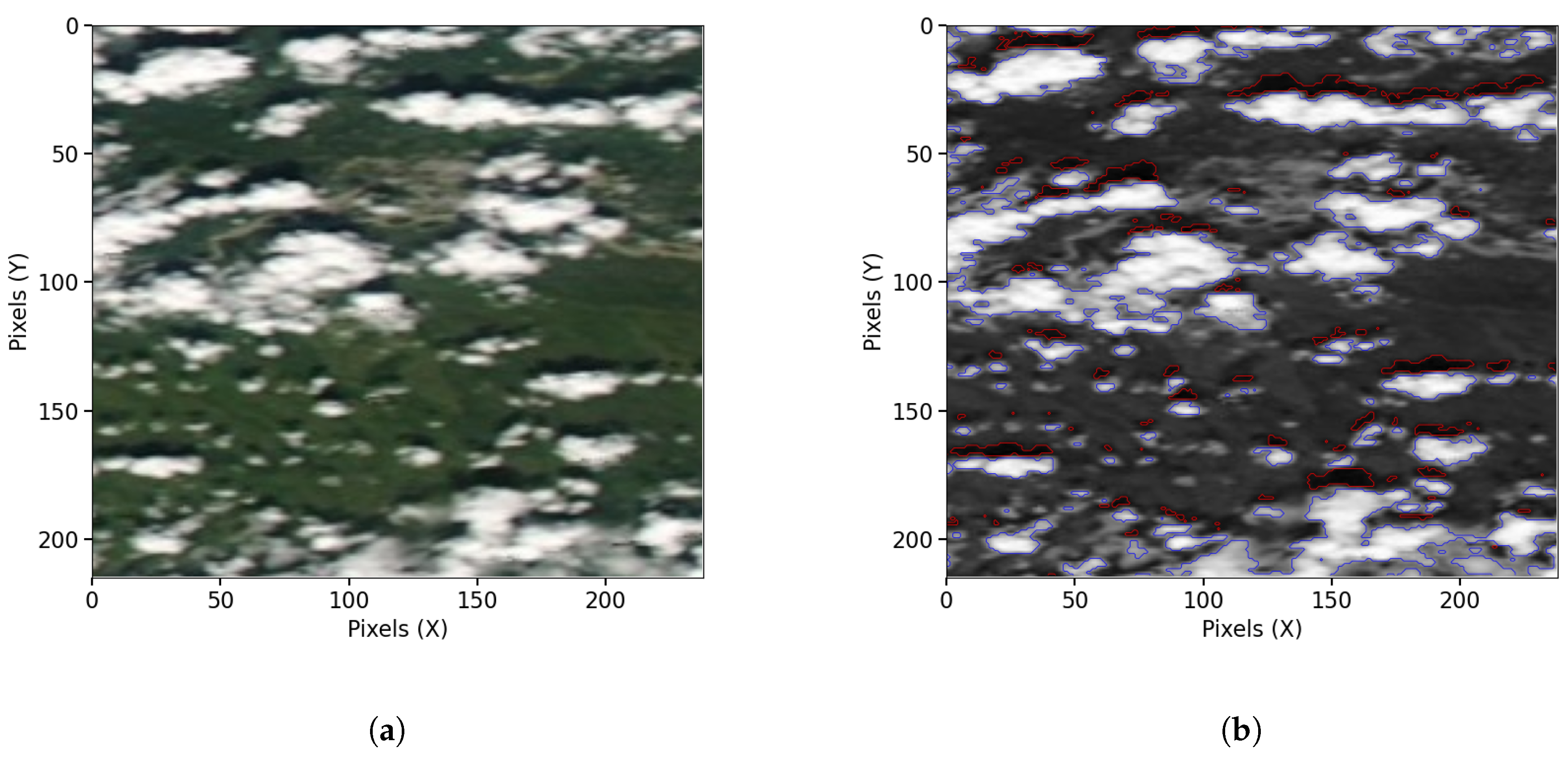
Figure 2.
MODIS Aqua imagery over Fairbanks, Alaska, on 26 July 2021. (2(a)) shows shallow, fair-weather cumulus humilis clouds observed at 21:34 UTC, used to demonstrate a shadow-based cloud base height retrieval technique under clear-sky conditions. (2(b)) builds on this example and illustrates the KD-tree-based cloud–shadow matching approach, with cloud masks outlined in blue and shadow masks in red.
2.2. Data
The Moderate Resolution Imaging Spectroradiometer (MODIS) is a key instrument aboard NASA’s Terra (launched in 1999) and Aqua (launched in 2002) satellites. The MOD02QM (Terra) and MYD02QM (Aqua) products contain calibrated radiance data from the 250 m resolution bands (Bands 1 and 2), primarily in the red and near-infrared wavelengths. These products offer 5-minute granules of Level-1B radiance data, ideal for high-resolution analysis of cloud optical and geometric properties, including shadow-based cloud base height estimation. Terra (MODIS) crosses the equator at approximately 10:30 AM local time (descending node), while Aqua (MODIS) crosses at around 1:30 PM (ascending node), enabling synergistic morning and afternoon observations. Cloud height information was compared against collocated MPLNET (Micro-Pulse Lidar Network) measurements [14]. Version 3 MPLNET lidar data were used here to provide information on atmospheric vertical structure and aerosol height and backscatter properties [15]. The MPLNET data are available online at https://mplnet.gsfc.nasa.gov, accessed on 7 November 2024. Radiosonde profiles were used to provide independent atmospheric validation and to confirm that the shadow length corresponds to cloud base height rather than cloud top height. Sounding data were obtained from the University of Wyoming’s Upper Air Archive, which offers a global, long-term dataset of radiosonde observations. These include vertical profiles of temperature, pressure, humidity, and wind, typically launched twice daily at 00 and 12 UTC. For this study, radiosonde measurements from the Bet Dagan station in Israel (WMO ID: 40179) launched at 12 UTC were used to closely coincide with the MODIS Aqua overpass time, allowing evaluation of the thermodynamic consistency of MODIS-derived cloud base heights and estimation of the lifting condensation level (LCL) under clear-sky conditions. The sounding data are publicly available at https://weather.uwyo.edu/upperair/sounding.shtml (accessed on November 7, 2024).
3. Results
To illustrate the effectiveness of the cloud shadow technique, we selected three geographically diverse locations: Bet Dagan, Sde Boker, and Fairbanks discussed in Table 1. These sites represent a range of terrains, from the Mediterranean coastal plain of Bet Dagan, to the arid highlands of Sde Boker in the Negev Desert, and the subarctic landscape of Fairbanks, Alaska. Despite their differing climates and surface characteristics, all three locations share a common feature: relatively low elevation. This characteristic is particularly advantageous for applying the cloud shadow method, as it minimizes uncertainties related to terrain-induced parallax or elevation corrections, thereby enhancing the accuracy of cloud base height estimations from satellite imagery.
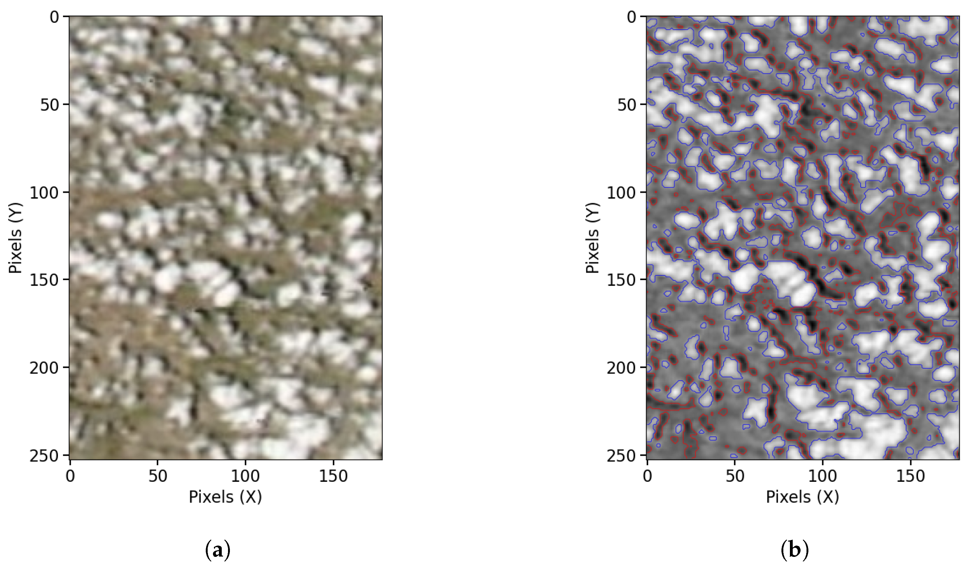
Figure 3.
MODIS Aqua imagery over Sde Boker, Israel, on 4 September 2024. (3(a)) shows shallow, fair-weather cumulus humilis clouds observed at 11:32 UTC, used to demonstrate a shadow-based cloud base height retrieval technique under clear-sky conditions. (3(b)) builds on this example and illustrates the KD-tree-based cloud–shadow matching approach, with cloud masks outlined in blue and shadow masks in red.
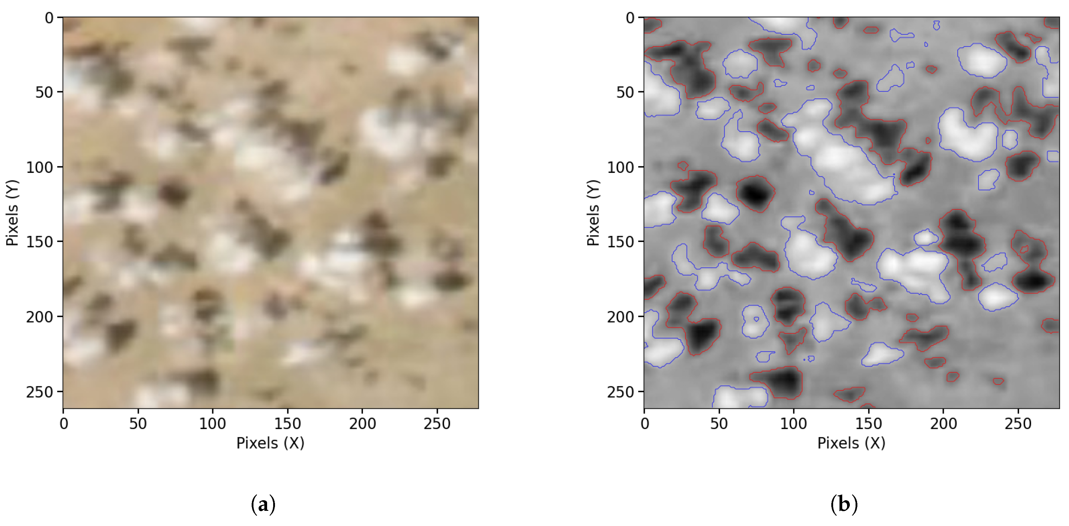
Figure 4.
MODIS Aqua imagery over Bet Dagan, Israel, on 26 April 2025. (4(a)) shows shallow, fair-weather cumulus humilis clouds observed at 12:04 UTC, used to demonstrate a shadow-based cloud base height retrieval technique under clear-sky conditions. (4(b)) builds on this example and illustrates the KD-tree-based cloud–shadow matching approach, with cloud masks outlined in blue and shadow masks in red.
3.1. Base Height and Shadow Length
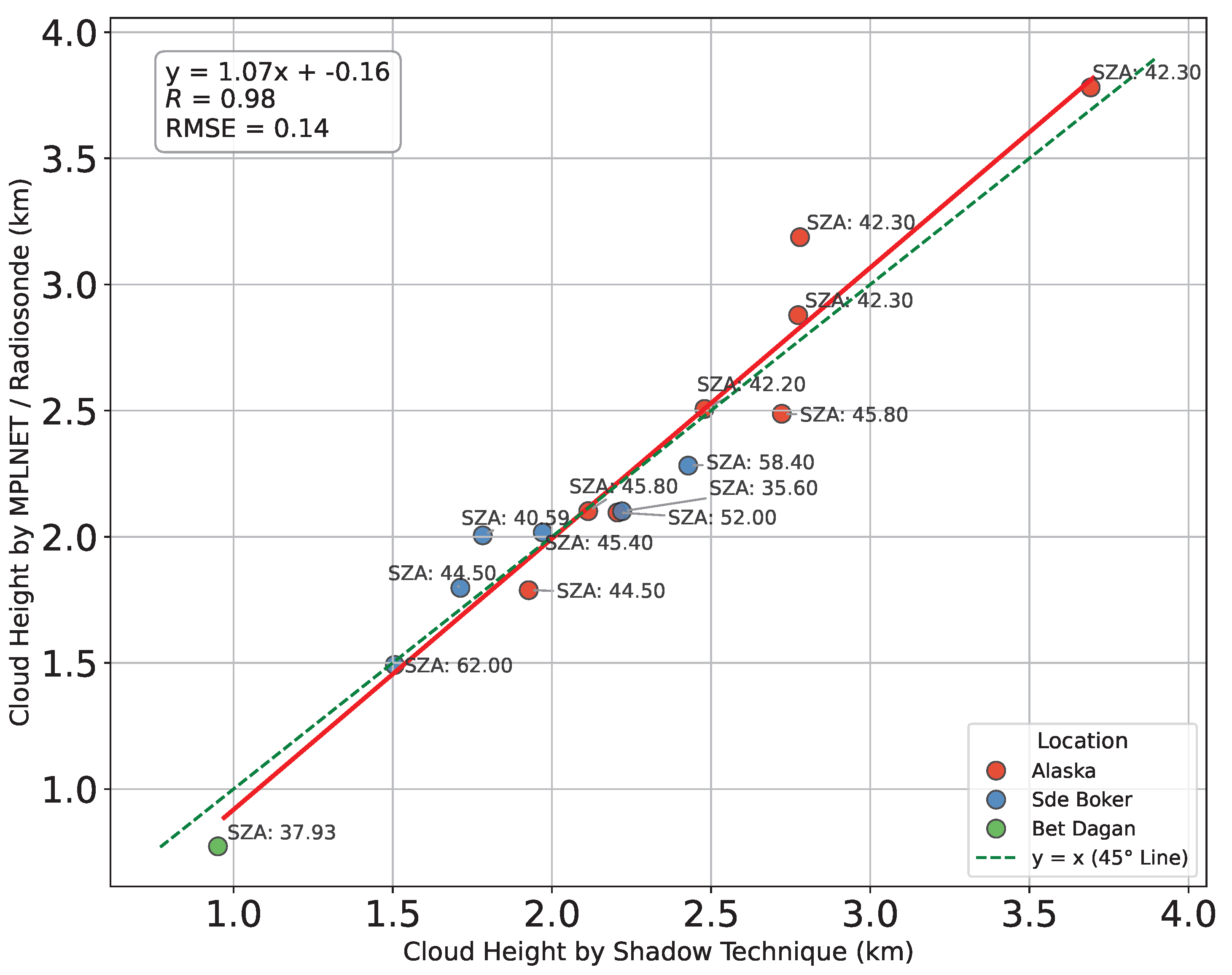
A strong agreement is observed between cloud base heights derived using the shadow-based technique and those measured by MPLNET and radiosonde, as shown in the Figure 5. The tight clustering of points around the 1:1 reference line highlights the high accuracy of the shadow method. The high correlation (R = 0.96) and low RMSE (0.14 km or 140 m) further confirm the reliability of the approach across different sites and solar geometries, as indicated by the varying solar zenith angles labeled beside each point. This small deviation lies within the expected geometric uncertainty given the spatial resolution of MODIS and variations in solar zenith angle. The radiosonde observation from Bet Dagan (26 April 2025) also supports the interpretation that the shadow-based method retrieves cloud base height rather than cloud top. This agreement provides crucial validation, confirming that the shadow technique aligns with vertically resolved in-situ atmospheric profiling. Overall, these findings demonstrate that the shadow-based method is a cost-effective and reliable alternative for estimating cloud base height in regions lacking active remote-sensing instruments.
Figure 5.
Scatter plot showing the relationship between cloud base height estimated using the shadow-based technique and collocated lidar-derived or radiosonde-measured cloud base heights. The solid line represents the 1:1 reference, while the dashed line indicates the linear regression fit. Correlation coefficient (R), root mean square error (RMSE), and regression equation are provided to assess the performance of the shadow-based method relative to lidar and radiosonde observations.
3.2. Applications
Diurnal Study Over Land
The diurnal study uses the Sde Boker location instead of Fairbanks, Alaska, primarily due to differences in latitude. Being at a higher latitude, Fairbanks has MODIS images from Aqua and Terra satellites captured within 1 to 1.5 hours of each other, whereas at Sde Boker, the time difference between images is about 3.5 hours. This larger temporal gap allows for a clearer comparison of cloud formation between morning and afternoon. Table 2 illustrates the diurnal evolution of cloud base heights over Sde Boker on September 4 and 21, 2024. On both days, early morning (around 08:00 UTC) cloud bases were measured at approximately 1.5 km by MPLNET, followed by a noticeable increase during late morning (around 11:30 UTC) to 2.1 km on September 4 and 2.0 km on September 21. These observations reflect the typical rise in cloud base height due to daytime boundary layer development. The consistent pattern across both days highlights the influence of surface-driven vertical mixing on cloud formation processes in arid environments under clear-sky conditions.

Table 2.
Cloud base heights retrieved from the shadow technique and MPLNET for two diurnal cases at Sde Boker.
Table 2.
Cloud base heights retrieved from the shadow technique and MPLNET for two diurnal cases at Sde Boker.
| Date | Time (UTC) | SZA (°) | MPLNET Height (km) | Shadow Height (km) |
|---|---|---|---|---|
| 2024-09-04 | 08:03 | 32.9 | 1.5 | 1.0 |
| 2024-09-04 | 11:32 | 35.6 | 2.1 | 2.2 |
| 2024-09-21 | 07:58 | 37.4 | 1.5 | 1.2 |
| 2024-09-21 | 11:27 | 40.6 | 2.0 | 1.8 |
Under convective conditions, where cloud formation typically occurs near the top of the mixed layer, cloud base height estimates from the cloud Shadow technique may also serve as a proxy for PBL height as evident from Figure 6. This makes it a potentially valuable tool for studying boundary layer processes in data-sparse regions or when direct vertical profiling is unavailable.
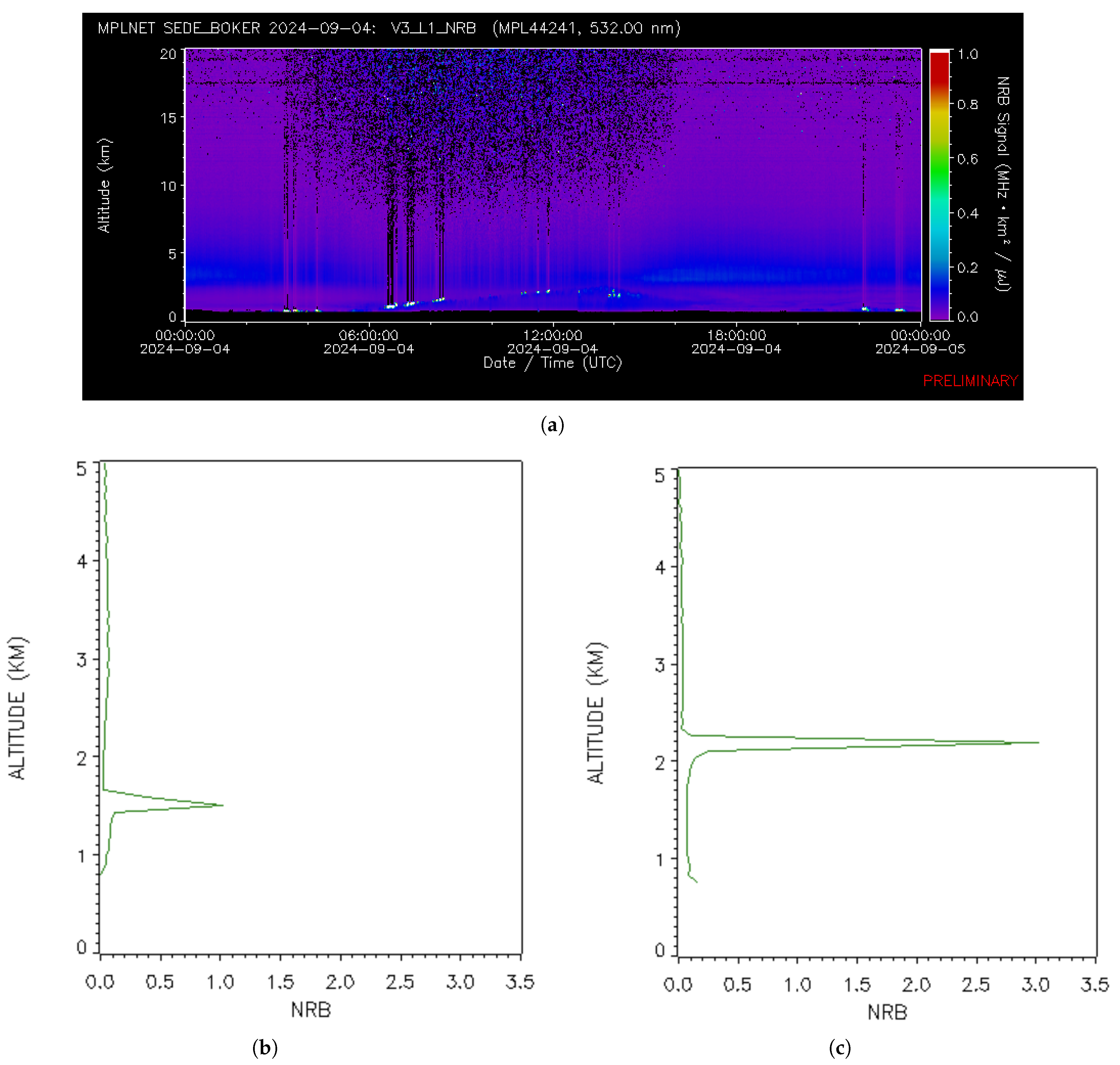
Figure 6.
MPLNET SEDE BOKER data from 2024-09-04. (6(a)) shows the full-day normalized relative backscatter signal. (6(b)) shows the aerosol backscatter profile at 08:03 UTC. (6(c)) shows the aerosol backscatter profile at 11:32 UTC.
Study Over Water Over the open ocean, the generally dark and homogeneous background can make cloud–shadow detection challenging, as the radiance contrast between shadowed and non-shadowed water is often weak. However, in regions affected by sun glint, the specular reflection from the ocean surface enhances the brightness of the background. This creates a sharper contrast between shadowed and illuminated areas, allowing the shadow technique to more reliably identify and track cloud shadows. Consequently, sun-glint regions are particularly well suited for the KD-tree-based cloud–shadow matching approach to retrieve cloud base heights as shown in Figure 7.
Figure 7.
MODIS Aqua imagery acquired over the ocean on 3 January 2024 at 21:03 UTC near latitude and longitude . (7(a)) shows the original MODIS Aqua image over the ocean, illustrating cloud formations. (7(b)) shows the corresponding cloud and shadow masks with cloud boundaries outlined in blue and shadow regions in red, illustrating the KD-tree-based cloud–shadow matching approach used to quantify their spatial displacement over water and retrieve cloud base height.
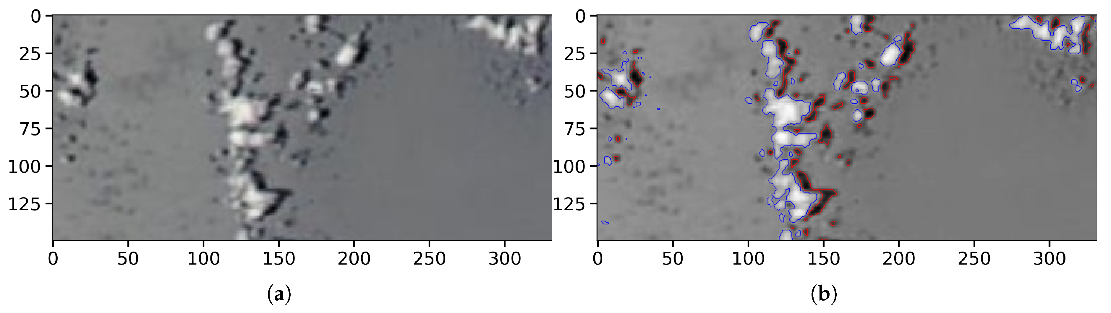
Table 3 presents cloud base heights (CBH) estimated using the shadow projection method applied to MODIS imagery, in conjunction with sea surface temperature (SST), relative humidity (RH), and wind speed from MERRA-2. The shadow technique infers CBH by exploiting the geometry between cloud shadows and the solar position. Across the three oceanic sites, SST increases and RH decreases toward the equator. The highest CBH (0.84 km) occurs at the subtropical site (), coinciding with moderate SST and the lowest wind speed (3.5 m s−1), conditions that may favor deeper cloud development. At the tropical site (), two CBH values (0.52 and 0.71 km) are retrieved, reflecting spatial variability and suggesting a mixture of shallow and deeper cumulus clouds. These results highlight the sensitivity of CBH to local thermodynamic conditions and underscore the utility of spatially resolved estimates over coarse grid averages.
4. Discussions
4.1. Diurnal Variations
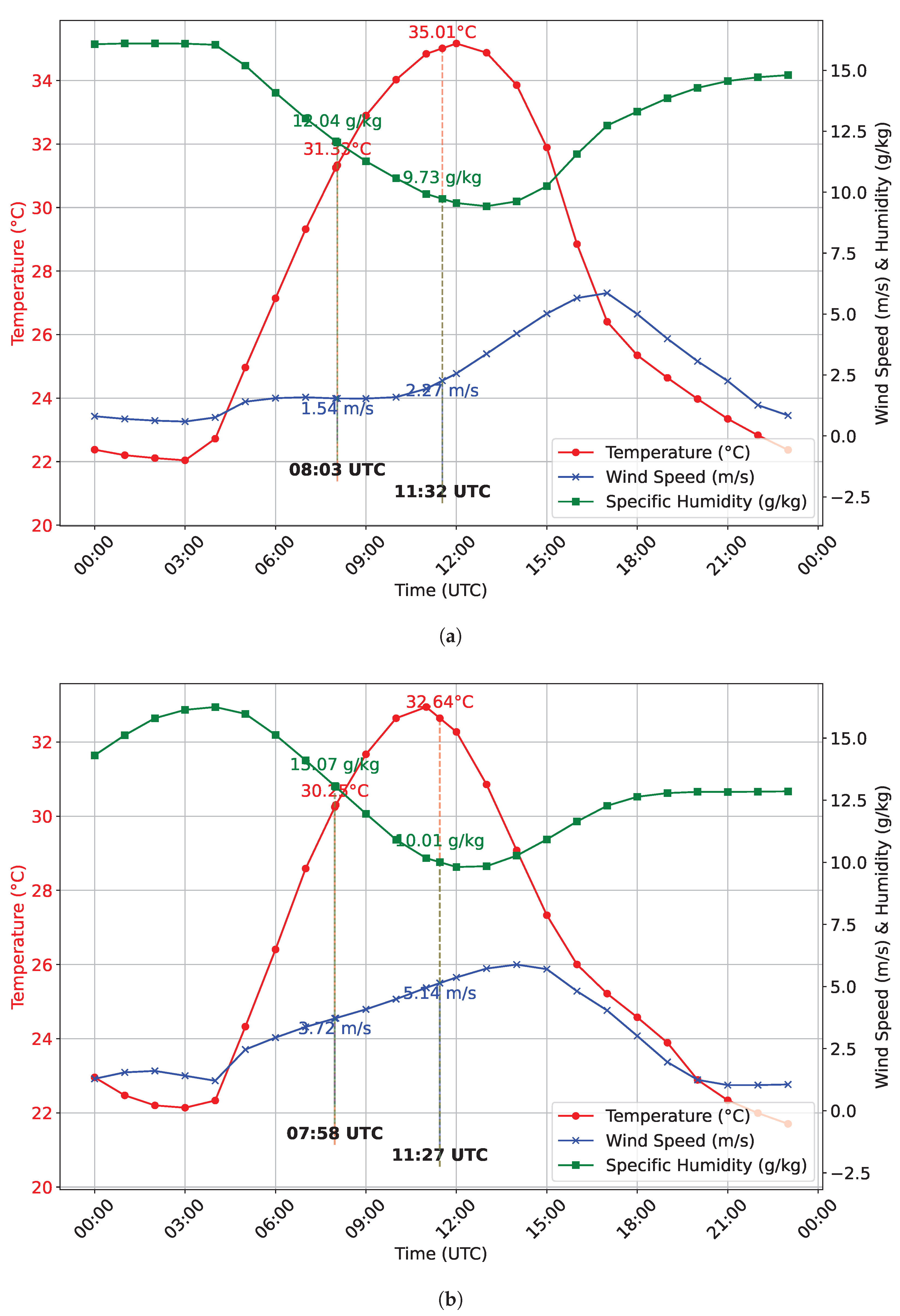
To further investigate the diurnal influence on cloud base height (CBH), MERRA-2 reanalysis data for two representative dates: September 4, 2024, and September 21, 2024 has been analyzed (Figure A1). These dates correspond to clear-sky days observed over the hyper-arid region of Sde Boker, Israel. Meteorological variables such as 2-meter air temperature (), specific humidity (), surface pressure (), and wind speed () were extracted from hourly MERRA-2 files at the closest grid point. Temporal interpolation was applied to estimate conditions at selected morning and early afternoon times.
The surface meteorological conditions over Sde Boker on September 4, 2024, exhibit clear diurnal evolution between early morning (08:03 UTC) and late morning (11:32 UTC). Air temperature rises significantly from 31.33 °C to 35.01 °C, consistent with daytime surface heating. Concurrently, specific humidity decreases from 12.04 g/kg to 9.73 g/kg, indicating a drying of the lower atmosphere, likely due to increased entrainment of drier air and vertical mixing. Surface pressure also shows a slight decline from 980.84 hPa to 978.46 hPa, a typical daytime pattern associated with warming and boundary layer deepening. Wind speed increases modestly from 1.54 m/s to 2.27 m/s, enhancing turbulent mixing in the boundary layer. The dew point drops from 16.58 °C to 13.25 °C, further reflecting the transition toward a drier and more well-mixed lower troposphere by midday. Similar pattern is also observed on September 21, 2024. These trends collectively illustrate the expected progression of surface-layer thermodynamics under clear-sky conditions during the late morning hours in a desert environment.
The meteorological conditions at the 2-meter level are further used to get CBH using the Equations (A1)–(A4) and the results are presented in Table 4.
Table 4 presents the cloud base height (CBH) predictions from three complementary methods: the Lifted Condensation Level (LCL) estimate, MPLNET lidar measurements, and the Cloud Shadow technique. This comparison provides a direct assessment of the shadow-based retrieval against both theoretical and observational benchmarks. The LCL provides a theoretical estimate of CBH derived from surface thermodynamic conditions, specifically temperature, humidity, and pressure. As such, it serves as a useful proxy, especially under well-mixed boundary layer conditions. However, the LCL assumes idealized adiabatic lifting without accounting for complex vertical mixing, atmospheric stability, or inversion layers, which often influence actual cloud formation heights. In contrast, MPLNET lidar observations deliver direct, high-resolution measurements of cloud base by detecting the vertical structure of aerosols and clouds, thereby capturing real atmospheric layering and mixing. This is reflected in the data, where MPLNET values tend to be slightly lower or differ from the LCL estimates, particularly during afternoon observations on September 21, 2024, suggesting the presence of vertical mixing or other atmospheric effects not captured by LCL.
The cloud shadow technique, which utilizes satellite imagery to estimate cloud base height, produces CBH values closely aligned with MPLNET measurements. This method is particularly valuable in data-sparse regions or locations where meteorological information is limited or unavailable such as remote terrestrial areas or even other planets, offering an alternative approach for cloud base estimation when ground-based instruments or atmospheric profiles are inaccessible. The accuracy of the Cloud Shadow technique can be further enhanced with improved spatial and temporal resolution of satellite data, allowing finer-scale atmospheric features to be captured. Overall, while the LCL method remains a useful and accessible estimate of cloud base height, lidar-based observations and satellite-derived techniques like Cloud Shadow offer more accurate, context-sensitive measurements by incorporating actual atmospheric conditions beyond surface thermodynamics. Moreover, the Cloud Shadow technique holds an advantage over lidar by providing broader spatial coverage and the ability to monitor cloud base height continuously across large and remote areas, making it an invaluable tool where deploying lidar systems is impractical. These diurnal patterns highlight how the shadow-based CBH retrieval effectively tracks boundary-layer development under clear-sky convective regimes.
4.2. Application to Hunga Tonga–Hunga Ha’apai
The geometric shadow-projection framework described here extends naturally beyond boundary-layer clouds to other atmospheric and planetary contexts. In particular, the Cloud Shadow technique is especially valuable for analyzing rare, transient events captured in only a handful of snapshot images, such as the 2022 Hunga Tonga–Hunga Ha’apai (HTHH) eruption or brief planetary flybys, where active sensors or multi-angle imaging are unavailable. In these situations, the presence of a distinct shadow provides a direct geometric constraint on vertical extent, enabling rapid, physically based height estimation from single-pass observations. Similar approaches have been demonstrated in JunoCam imagery of Jupiter, where bright “pop-up” clouds cast discernible shadows on deeper decks, revealing three-dimensional convective structure [4,5]. The ability to extract vertical information from purely optical data highlights the broad utility of shadow-based retrievals across both terrestrial and extraterrestrial environments, providing a unifying geometric perspective for cloud and plume height analysis.
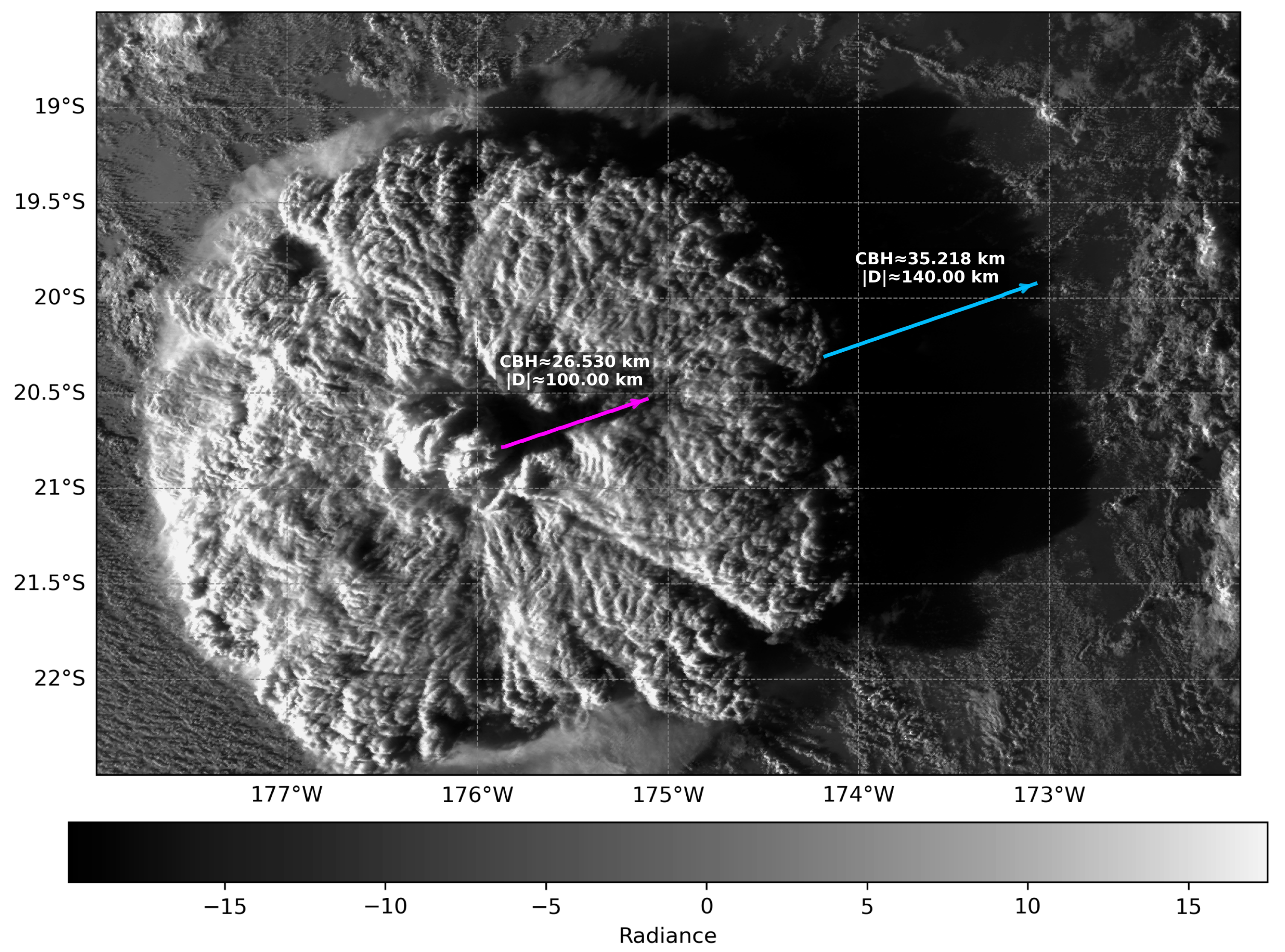
An immediate and illustrative application of this geometric framework is volcanic plume height retrieval. As shown in Figure 8 and Figure 9, the HTHH eruption exhibited sharply defined shadows across the ocean surface in consecutive GOES–17 images at 04:30 and 04:50 UTC. At 04:30 UTC, the plume displayed a prominent trident-shaped overshooting top with two distinct levels—approximately 18.4 km near the vent and 42.3 km along the distal edge—derived using the shadow-displacement geometry described in Section 2, with the explicit height-retrieval formulas provided in Appendix B. These values closely align with the dual-deck structure reported by Carr et al. [16] from GOES–Himawari stereo analysis for the same interval. By 04:50 UTC, the retrieved heights had decreased to about 26.5 km and 35.2 km, consistent with the lower-deck height of roughly 30 km noted by Carr et al., although their study did not capture the transient trident morphology evident in the GOES–17 projection. This temporal evolution reflects the gradual collapse and spreading of the upper overshooting top into a more stratified structure as the eruption weakened.
Figure 8.
GOES-17 visible imagery of the Hunga Tonga–Hunga Ha’apai eruption on 15 January 2022 at 04:30 UTC. The plume’s shadow projected on the ocean surface enables direct geometric estimation of its vertical extent using the shadow-based technique, where D denotes the haversine distance between the cloud and shadow latitude–longitude coordinates. The inner and outer arrows indicate retrieved plume heights of approximately 18.4 km and 42.3 km, respectively.
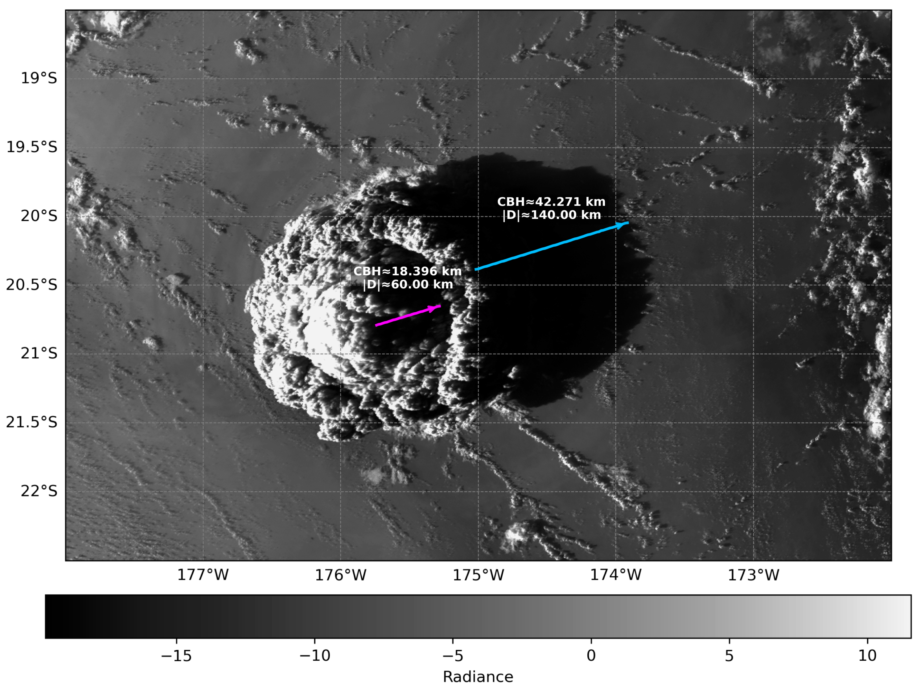
Figure 9.
Same as Figure 8, but for 15 January 2022 at 04:50 UTC. The inner and outer arrows indicate approximately 26.5 km and 35.2 km, respectively, reflecting the gradual collapse and settling of the eruption column over time.
Figure 9.
Same as Figure 8, but for 15 January 2022 at 04:50 UTC. The inner and outer arrows indicate approximately 26.5 km and 35.2 km, respectively, reflecting the gradual collapse and settling of the eruption column over time.
It is important to recall that earlier in this study the concept of the cloud aspect ratio was introduced, which describes the relationship between the vertical and horizontal dimensions of a cloud. The shadow-based method performs reliably for shallow boundary layer clouds that have small aspect ratios, but the HTHH plume represents an extreme case with a very large aspect ratio. The towering trident-shaped feature of the eruption column requires additional geometric caution because the apparent shadow displacement is influenced not only by the true vertical extent but also by the satellite viewing angle. For such tall plumes, this geometric distortion, known as satellite parallax, can lead to underestimation of the true height, particularly at oblique viewing angles where the shadow and sub-satellite projections differ. To address this, the present study applies a parallax-corrected haversine formulation (Appendix B) that accounts for Earth curvature and the satellite view geometry. Incorporating this correction ensures physically consistent and temporally coherent plume height estimates from geostationary imagery. When applied to time-sequenced satellite observations, this approach provides rapid, physics-based estimates of plume ascent, umbrella formation, and dispersal altitude, offering valuable insights for volcanic monitoring and atmospheric hazard assessment.
Building on this application, the KD-tree-based matching framework used here remains inherently two-dimensional. When augmented with three-dimensional information such as digital elevation models or lidar-derived canopy height models, however, it could extend beyond simple shadow–object matching. This would allow not only more accurate cloud–shadow association over complex terrain, but also structural assessments of terrestrial targets. In ecological studies, for example, such an approach could support tree detection together with biomass and carbon stock estimation, as demonstrated in high-resolution mapping of African dryland trees [17]. More broadly, the same strategy could be applied to planetary surfaces, where shadows cast by dust plumes, volcanic eruptions, or ice features could be paired with surface topography to retrieve height and volume information, extending the method’s utility from Earth system science to planetary exploration.
4.3. High-Resolution Images
Furthermore, utilizing high-resolution satellite imagery from sources such as Planet Labs, Maxar, and Google can significantly enhance the accuracy of the Cloud Shadow technique for estimating cloud base height. The improved spatial resolution allows for more accurate detection and measurement of cloud shadows, reducing uncertainties associated with lower-resolution data. This advancement enables finer-scale analysis and more reliable cloud base height estimates, as illustrated in the satellite images referenced in Figure 10.
Together, these analyses from diurnal boundary-layer evolution to stratospheric plumes and high-resolution imaging demonstrate the adaptability of the shadow-based framework across scales and atmospheric regimes.
5. Conclusion
This study demonstrates the effectiveness of a shadow-based remote sensing approach for estimating planetary boundary layer (PBL) cloud base height (CBH) using MODIS visible imagery. By combining cloud–shadow displacement with solar geometry, the method directly estimates CBH from geometry, without requiring cloud-top information, stereo imaging, or active sensors. Validation against collocated MPLNET lidar and radiosonde measurements shows strong agreement (, RMSE km or 140 m), confirming the reliability of the approach for shallow, isolated cumulus clouds.
The technique successfully captures diurnal variations in cloud development, with cloud bases observed to rise from morning to afternoon in response to boundary layer deepening and enhanced convection. As surface heating progresses, moist parcels are mixed upward until reaching the lifting condensation level, forming clouds at higher altitudes later in the day. This consistency with boundary-layer thermodynamics underscores the physical robustness of the approach.
Results over the ocean further demonstrate the method’s ability to resolve spatial variability in CBH under different surface and atmospheric conditions (Table 3). Higher humidity and cooler sea surface temperatures were associated with shallower cloud bases, while drier conditions and weaker winds coincided with deeper boundary layers and higher CBH. The tropical case revealed mixed shallow and moderately developed cumuli, highlighting the technique’s sensitivity to local forcing and its utility for capturing cloud variability across marine environments.
The same geometric principle was extended to high-altitude volcanic plumes, as illustrated for the Hunga Tonga–Hunga Ha’apai eruption. By computing the great-circle (haversine) distance between plume and shadow coordinates and applying parallax correction for oblique viewing geometry, the method retrieved physically consistent multi-level plume heights from GOES-17 imagery. This extension demonstrates the scalability of the shadow-based technique from low-level boundary-layer clouds to stratospheric plume analysis.
Although the method is limited by solar geometry, terrain complexity, and shadow ambiguity, these challenges can be mitigated through higher-resolution satellite sensors (e.g., Sentinel-2, PlanetScope, WorldView) and automated shadow detection. The increasing availability of such data opens opportunities to extend the approach beyond CBH retrieval to plume height estimation, volcanic ash monitoring, vegetation structure analysis, and urban feature mapping. Future work should focus on extending validation to diverse climates and seasons, as well as exploring machine learning techniques to improve retrievals under suboptimal conditions.
Overall, the shadow-based technique provides direct geometric estimates of CBH without requiring atmospheric profiles or active sensors. The method’s low computational cost and reliance on widely available satellite data make it a valuable tool for atmospheric research, weather forecasting, renewable energy, and planetary science applications. Future research should explore integration with AI-based cloud segmentation to extend retrievals to multilayer scenes and coastal transition zones.
Author Contributions
Conceptualization, L.M. and D.L.W.; methodology, L.M. and D.L.W.; software, L.M.; validation, L.M. ; formal analysis, L.M. and D.L.W.; investigation, L.M. and D.L.W.; resources, L.M. and D.L.W.; writing—original draft preparation, L.M.; writing—review and editing, L.M., D.L.W.; visualization, L.M.; supervision, D.L.W.; project administration, D.L.W; funding acquisition, D.L.W. All authors have read and agreed to the published version of the manuscript.
Funding
This research was funded by Total and Spectral Solar Irradiance Sensor (TSIS) and Sun-Climate Research Supports to GSFC.
Acknowledgments
The MODIS MYD02QKM data used in this study were obtained from the NASA Level-1 and Atmosphere Archive and Distribution System (LAADS) Distributed Active Archive Center (DAAC), maintained by the NASA Goddard Space Flight Center. The MERRA-2 reanalysis data were provided by the Global Modeling and Assimilation Office (GMAO) at NASA Goddard Space Flight Center through the NASA Goddard Earth Sciences Data and Information Services Center (GES DISC). MPLNET lidar data were provided by the Micro-Pulse Lidar Network, managed by the NASA Goddard Space Flight Center. . The authors also gratefully acknowledge the University of Wyoming Department of Atmospheric Science for providing the radiosonde data used in this study. PlanetScope imagery was used for demonstration purposes and provided by Planet Labs PBC under their research data access program.
Conflicts of Interest
The authors declare no conflicts of interest.
Appendix A Estimation of Cloud Base Height (CBH) from Surface Meteorological Variables
Figure A1.
Surface-layer meteorological variables at Sde Boker from MERRA-2 data. (a) shows data for 2024-09-04, with highlighted times at 08:03 UTC and 11:32 UTC. (b) shows data for 2024-09-21, with highlighted times at 07:58 UTC and 11:27 UTC. In each case, temperature, specific humidity, and wind speed at 2m are shown, with key profiles marked by dashed lines and annotated values.
The cloud base height (CBH) is an important atmospheric parameter that can be estimated using surface temperature, humidity, and pressure data. This section details the method used to compute CBH based on meteorological variables extracted from NetCDF data.
The calculation begins by converting the specific humidity q (kg/kg) to the mixing ratio w, defined as the mass of water vapor per mass of dry air, using the relation ([18]):
Next, the vapor pressure e (in hPa) is calculated from the mixing ratio w and the surface pressure P (hPa) by ([18]):
The dew point temperature (°C) is then computed from the vapor pressure e using the Magnus formula [19]:
Finally, the cloud base height in meters is estimated by relating the temperature difference between the surface air temperature T and the dew point temperature as ([20,21]):
Here, the temperature values T and are given in degrees Celsius.
Meteorological data including 2-meter air temperature , specific humidity , surface pressure , and wind components at 2 meters and , are extracted from the MERRA-2 NetCDF files at the closest grid point to the target location. The temperature and specific humidity are converted from Kelvin to Celsius and from kg/kg to g/kg, respectively, and pressure from Pascal to hectopascal.
To align the data with specific target times (e.g., 08:03 UTC and 11:32 UTC), linear interpolation is applied to all variables, allowing precise temporal estimates of the meteorological conditions.
Using the interpolated temperature, humidity, and pressure data, the dew point temperature is calculated via Equation A3, followed by the cloud base height estimation using Equation A4. Wind speed at 2 meters is also computed as
The resulting CBH values provide insight into the vertical structure of the atmosphere and can be used in conjunction with other observational data to analyze cloud formation processes.
Appendix A Shadow–Plume Height Retrieval Formulation
The height retrieval formulation used in this study follows the geometric framework described as Method 3 in [22], with a key modification in how the horizontal distance between the plume edge (P) and its corresponding shadow edge (S) is computed. Instead of relying on planar angular separation, the present approach uses the haversine distance between latitude–longitude pairs, which inherently accounts for Earth’s curvature.
Height Retrieval Under Nadir and Oblique Views
For near-nadir satellite viewing geometry, the vertical height H of the plume top above the surface can be estimated from the simple tangent relation:
where is the solar elevation angle at the time of observation.
For non-nadir or off-center viewing geometries (i.e., when the satellite view zenith angle is non-zero), parallax displacement must be considered. The corresponding expression becomes:
where is the satellite view zenith angle at the plume location.
In this formulation, D represents the haversine distance between the shadow and the cloud coordinates, as described below, whereas in Ákos (2021) it was expressed through angular displacements derived from image-plane geometry. By directly computing D from latitude–longitude navigation data, the present method avoids projection biases and ensures consistency across both nadir and oblique satellite views.
Haversine Distance Between Plume and Shadow
The great-circle distance D between the plume edge (P) at and the shadow edge (S) at is expressed as:
where is Earth’s mean radius (6,371 km), and and denote latitude and longitude (in radians), respectively. The computed D replaces the angular separation term used in [22], providing a more accurate measure of the true surface separation between the cloud and its shadow under varying geometries.
Comparison With Previous Methods
Earlier shadow-based height estimation approaches often assumed planar geometry, which neglects Earth’s curvature and can introduce systematic errors at large solar or viewing zenith angles. In this work, we employ the haversine formulation to represent the surface distance between the plume and its shadow, thereby explicitly incorporating the curvature of the Earth into the retrieval geometry. This refinement, combined with the view-dependent correction, enables accurate height estimation even under oblique observation conditions, as demonstrated in the GOES-17 analysis of the Hunga Tonga–Hunga Ha’apai eruption.
References
- Mishra, M.K.; Kalita, J.; Chauhan, P.; Kumar, R.; Sarkar, S.; Singh, R.; Guha, A. MCC’s First-Ever Observation of a High-Altitude Plume Cloud on Mars: Linkages with Space Weather? Journal of the Indian Society of Remote Sensing 2025, 53, 345–360. [Google Scholar] [CrossRef]
- Shaheen, F.; Scariah, N.V.; Lala, M.G.N.; Krishna, A.; Jeganathan, C.; Hoekzema, N. Shadow method retrievals of the atmospheric optical depth above Gale crater on Mars using HRSC images. Icarus 2022, 388, 115229. [Google Scholar] [CrossRef]
- Giacamán, C.A.R. High-Precision Measurement of Height Differences from Shadows in Non-Stereo Imagery: New Methodology and Accuracy Assessment. Remote Sensing 2022, 14, 1702. [Google Scholar] [CrossRef]
- Hansen, C.J.; Caplinger, M.A.; Ingersoll, A.P.; Ravine, M.A.; Jensen, E.; Bolton, S.J.; Orton, G.; Reuter, D.; Simon, A.A.; Tabataba-Vakili, F.; et al. JunoCam: Juno’s Outreach Camera. Space Science Reviews 2017, 213, 475–506. [Google Scholar] [CrossRef]
- team, M. Jupiter’s Swirling Cloudscape. https://www.missionjuno.swri.edu/news/jupiters-swirling-cloudscape, 2018. Accessed 2025-11-04.
- Williams, A.P.; Gentine, P.; Moritz, M.A.; Roberts, D.A.; Abatzoglou, J.T. Effect of reduced summer cloud shading on evaporative demand and wildfire in coastal southern California. Geophysical Research Letters 2018, 45, 5653–5662. [Google Scholar] [CrossRef]
- Federal Aviation Administration. Aeronautical Information Manual, Chapter 3: Airspace, Section 2: Controlled Airspace, 2023.
- UK Civil Aviation Authority. Weather Minima for Visual Flight Rules (VFR), 2023.
- Wikipedia contributors. Visual Meteorological Conditions, 2024.
- Fretwell, P.T.; LaRue, M.A.; Morin, P.; Kooyman, G.L.; Wienecke, B.; Ratcliffe, N.; Fox, A.J.; Fleming, A.H.; Porter, C.; Trathan, P.N. An Emperor Penguin Population Estimate: The First Global, Synoptic Survey of a Species from Space. PLoS ONE 2012, 7, e33751. [Google Scholar] [CrossRef]
- Sengupta, S.K.; Berendes, T.; Welch, R.M.; Navar, M.; Wielicki, B.A. Automated cloud base height determination from high resolution Landsat data – A Hough transform approach. In Proceedings of the Conference on Atmospheric Radiation; 1990. [Google Scholar]
- Berendes, T.; Sengupta, S.K.; Welch, R.M.; Wielicki, B.A.; Navar, M. Cumulus cloud base height estimation from high spatial resolution Landsat data: a Hough transform approach. IEEE Transactions on Geoscience and Remote Sensing 1992, 30, 430–443. [Google Scholar] [CrossRef]
- Bentley, J.L. Multidimensional binary search trees used for associative searching. Communications of the ACM 1975, 18, 509–517. [Google Scholar] [CrossRef]
- Welton, E.J.; Campbell, J.R.; Spinhirne, J.D.; Scott III, V.S. Global monitoring of clouds and aerosols using a network of micropulse lidar systems. In Proceedings of the Lidar remote sensing for industry and environment monitoring. SPIE, Vol. 4153; 2001; pp. 151–158. [Google Scholar]
- Welton, E.J.; Stewart, S.A.; Lewis, J.R.; Belcher, L.R.; Campbell, J.R.; Lolli, S. Status of the NASA Micro Pulse Lidar Network (MPLNET): overview of the network and future plans, new version 3 data products, and the polarized MPL. In Proceedings of the EPJ Web of Conferences. EDP Sciences, Vol. 176; 2018; p. 09003. [Google Scholar]
- Carr, J.L.; Horváth, Á.; Wu, D.L.; Friberg, M.D. Stereo Plume Height and Motion Retrievals for the Record-Setting Hunga Tonga–Hunga Ha’apai Eruption of 15 January 2022. Geophysical Research Letters 2022, 49, e2022GL098131. [Google Scholar] [CrossRef]
- Tucker, C.; Brandt, M.; Hiernaux, P.; Kariryaa, A.; Rasmussen, K.; Small, J.; Igel, C.; Reiner, F.; Melocik, K.; Meyer, J.; et al. Sub-continental-scale carbon stocks of individual trees in African drylands. Nature 2023, 615, 80–86. [Google Scholar] [CrossRef] [PubMed]
- Wallace, J.M.; Hobbs, P.V. Atmospheric Science: An Introductory Survey, 2 ed.; Elsevier Academic Press: Amsterdam; Boston, 2006.
- Wikipedia contributors. Dew point. https://en.wikipedia.org/wiki/Dew_point, 2025. Accessed: 2025-08-07.
- Stull, R.B. An Introduction to Boundary Layer Meteorology; Springer: Dordrecht, 1988; p. 666. [Google Scholar] [CrossRef]
- Johnson, R.H.; Ciesielski, P.E. Potential Vorticity Generation by West African Squall Lines. Monthly Weather Review 2020, 148, 1691–1715. [Google Scholar] [CrossRef]
- Ákos Horváth. ; Carr, J.L.; Girina, O.A.; Wu, D.L.; Bril, A.A.; Mazurov, A.A.; Melnikov, D.V.; Hoshyaripour, G.A.; Buehler, S.A. Geometric estimation of volcanic eruption column height from GOES-R near-limb imagery – Part 1: Methodology. Atmospheric Chemistry and Physics 2021, 21, 12189–12206. [Google Scholar] [CrossRef]
Figure 1.
Illustration of cloud base height variability across Subtropical, Tropical, and Equatorial regions.
Figure 1.
Illustration of cloud base height variability across Subtropical, Tropical, and Equatorial regions.
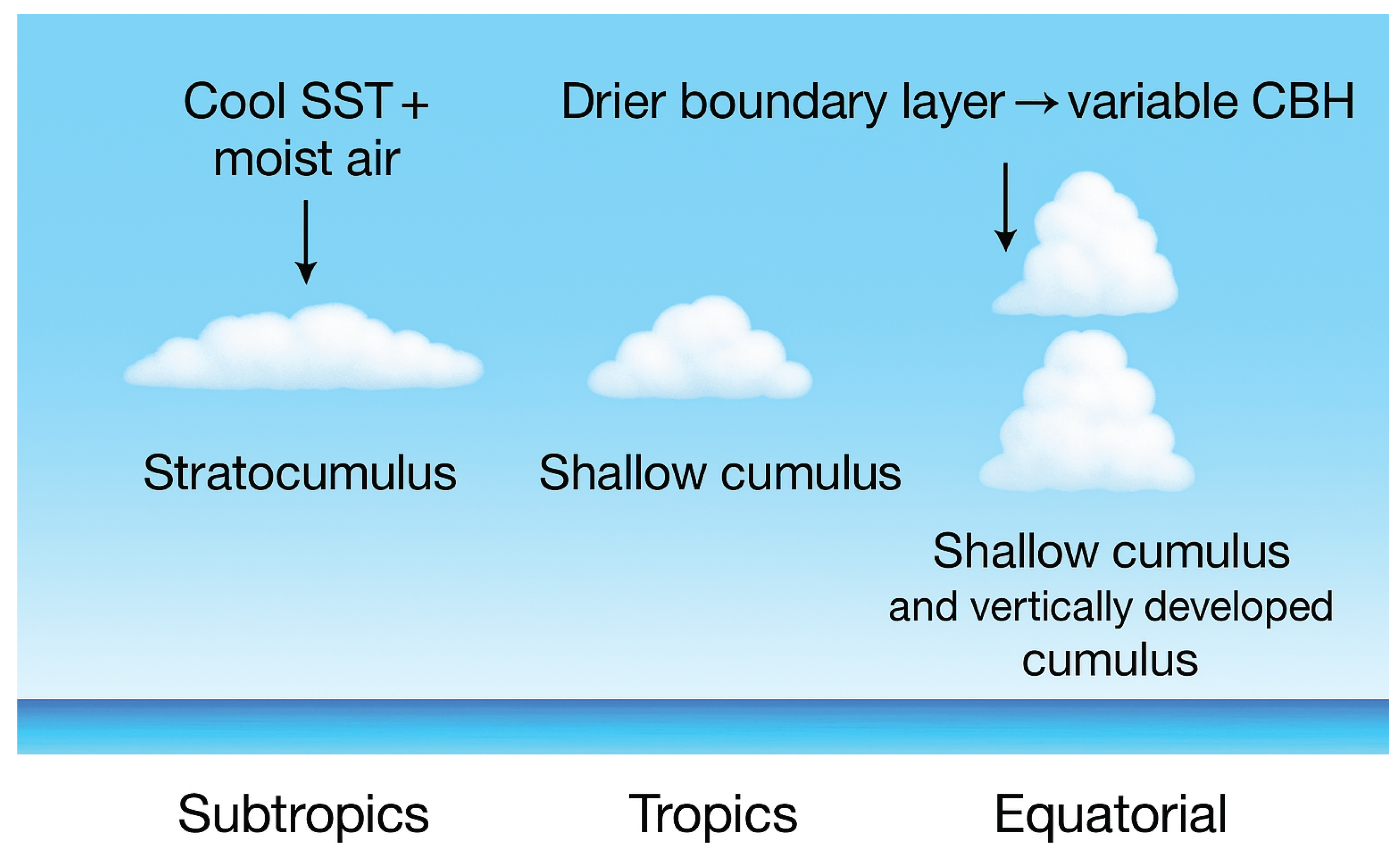
Figure 10.
PlanetScope satellite image of Momotombo volcano, Nicaragua, acquired on October 28, 2016. The image shows an active eruption, with a volcanic plume rising from the summit crater and dark lava flows extending down the flanks. Source: PlanetScope.
Figure 10.
PlanetScope satellite image of Momotombo volcano, Nicaragua, acquired on October 28, 2016. The image shows an active eruption, with a volcanic plume rising from the summit crater and dark lava flows extending down the flanks. Source: PlanetScope.
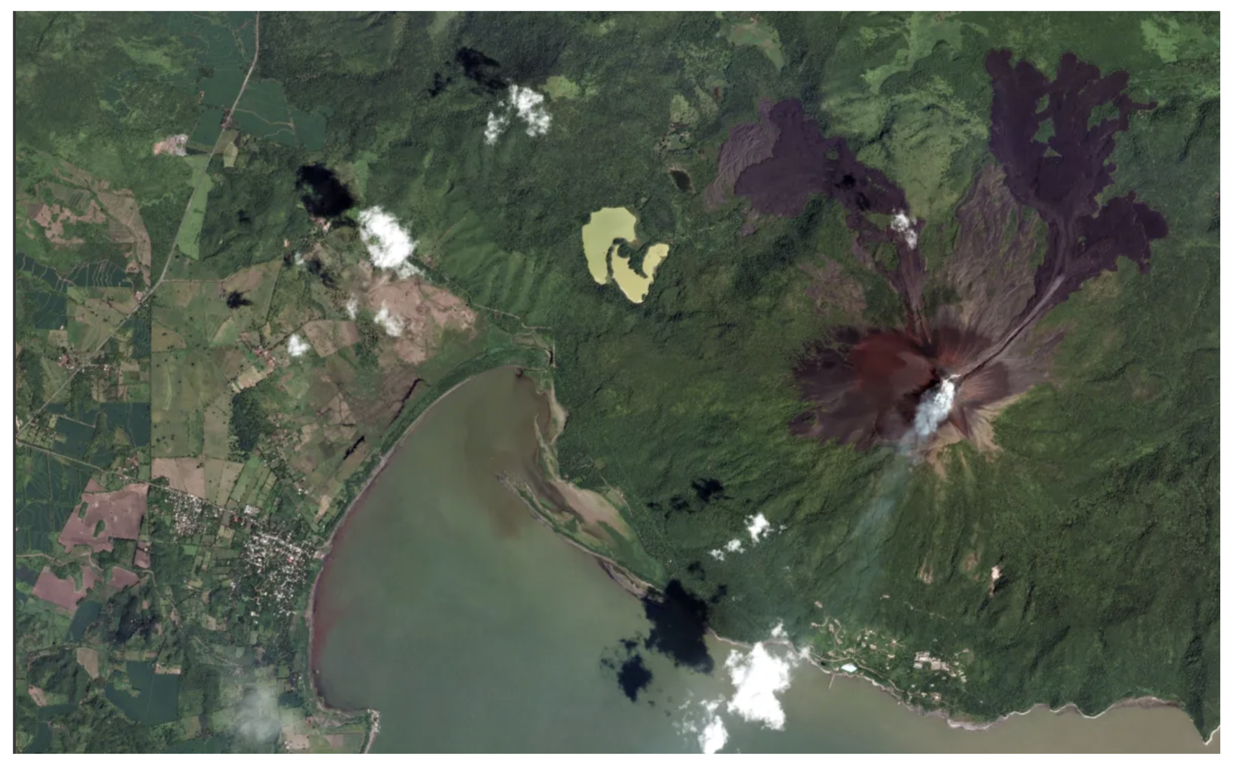
Table 1.
Selected Locations Under Study
| Location | Elevation (approx.) |
|---|---|
| Bet Dagan, Israel | 40 m (131 ft) |
| Sde Boker, Israel | 480 m (1,575 ft) |
| Fairbanks, Alaska | 136 m (446 ft) |
Table 3.
Cloud base height estimates from the shadow technique, with sea surface temperature (SST), relative humidity (RH), and wind speed from MERRA-2.
Table 3.
Cloud base height estimates from the shadow technique, with sea surface temperature (SST), relative humidity (RH), and wind speed from MERRA-2.
| Latitude | Longitude | SST | RH | Wind Speed | Cloud Shadow Height |
|---|---|---|---|---|---|
| (°) | (°) | (°C) | (%) | (m/s) | (km) |
| -28.905 | -102.343 | 22.1 | 81 | 6.1 | 0.550 |
| -19.693 | -104.795 | 23.6 | 76 | 3.5 | 0.840 |
| -7.347 | -108.099 | 26.2 | 67 | 7.4 | 0.520/0.71 |
Table 4.
CBH Predictions from LCL, MPLNET, and Cloud Shadow Techniques
| Local Date & Time | LCL Estimate | MPLNET | Cloud Shadow |
|---|---|---|---|
| (IDT) | (km) | (km) | (km) |
| Sep 4, 2024 – 10:58 (07:58 UTC) | 1.548 | 1.5 | 1.0 |
| Sep 21, 2024 – 11:03 (08:03 UTC) | 1.845 | 1.5 | 1.2 |
| Sep 4, 2024 – 14:27 (11:27 UTC) | 2.369 | 2.1 | 2.2 |
| Sep 21, 2024 – 14:32 (11:32 UTC) | 2.720 | 2.0 | 1.8 |
Disclaimer/Publisher’s Note: The statements, opinions and data contained in all publications are solely those of the individual author(s) and contributor(s) and not of MDPI and/or the editor(s). MDPI and/or the editor(s) disclaim responsibility for any injury to people or property resulting from any ideas, methods, instructions or products referred to in the content. |
© 2025 by the authors. Licensee MDPI, Basel, Switzerland. This article is an open access article distributed under the terms and conditions of the Creative Commons Attribution (CC BY) license (http://creativecommons.org/licenses/by/4.0/).
Copyright: This open access article is published under a Creative Commons CC BY 4.0 license, which permit the free download, distribution, and reuse, provided that the author and preprint are cited in any reuse.


