
Submitted:
19 November 2025
Posted:
20 November 2025
You are already at the latest version
Abstract
High‐resolution climate information is essential for risk assessment and adaptation, yet the gap between coarse Earth system model output and local scales persists. We synthesize machine‐learning (ML) approaches for climate downscaling from 2010--2025 across classical methods, convolutional super‐resolution, generative models (GANs/VAE--GANs), diffusion, and transformers. We highlight what each class actually delivers for practitioners—improvements in spatial structure, calibration, and depiction of extremes—alongside limitations that remain: sensitivity to training losses and data, non‐stationarity under warming, physical (in)consistency, and reliable uncertainty quantification. We connect methodological choices (e.g., residual vs.\ plain CNNs; intensity‐aware losses; spectra‐aware evaluation; ensemble generation) to changes in verified skill and failure modes.
Our assessment yields practical guidance: pair strong linear/bias‐correction baselines with structure‐ and tail‐aware metrics; stress‐test under warming; prefer probabilistic generators when ensembles are required; and evaluate multivariate coherence when multiple variables are downscaled. We close with priorities for the next decade: physics‐aware objectives, robust out-of distribution (OOD) detection and adaptation, scalable transfer across regions and resolutions, and trustworthy
evaluation protocols.
Keywords:
climate downscaling
; machine learning
; deep learning
; transferability
; physical consistency
; explainable AI
; uncertainty quantification
1. Introduction: The Imperative for High-Resolution Climate Projections and the Rise of Machine Learning
1.1. Positioning This Review in the Literature
While the application of machine learning (ML) to climate downscaling is a burgeoning field, this review provides a distinct and timely contribution by offering a broad, critical synthesis of methodologies, persistent challenges, and future research trajectories from 2010–2025. Our work differs from more focused empirical studies, such as the influential intercomparison by Vandal et al. [1], which conducted its own experiments to evaluate a specific set of ML methods for downscaling daily precipitation in a single region. Rather than performing a new empirical analysis, our review synthesizes the findings from a multitude of such studies across diverse variables, geographies, and model architectures.
Furthermore, our scope is broader than that of critical methodological papers like Rampal et al. [2], which delved deeply into the specific, vital challenge of model interpretability by demonstrating a visualization technique for a convolutional neural network. While we analyze and incorporate the insights from such explainability research, our aim is to assess the entire ecosystem of ML downscaling, from model selection to the representation of extremes and physical consistency.
Our review also complements recent comprehensive surveys like Rampal et al. [3], which provides an excellent overview of recent ML advancements, covers both observational downscaling and regional climate model (RCM) emulation, and discusses key research gaps and evaluation strategies. While Rampal et al. [3] provides an essential and comprehensive guide to recent advancements, our review builds upon this by offering a more critical synthesis structured specifically around the "performance paradox" and "trust deficit" to provide targeted, prescriptive guidance. This review offers a unique, consolidated synthesis for the contemporary deep learning era by:
- Creating a novel taxonomy that explicitly maps different classes of ML models—from CNNs and GANs to Transformers and Diffusion Models—to the specific downscaling challenges they are best suited to address.
- Conducting a critical analysis of the “performance paradox,” where high statistical skill on historical data often fails to translate to robust performance under the non-stationary conditions of future climate change.
- Proposing a practical evaluation protocol and charting clear, targeted research priorities to guide the community towards developing more physically consistent, trustworthy, and operationally viable models.
This positioning is further clarified by contrasting our work with other foundational papers. Foundational reviews like Maraun et al. [4] covered the state of the art before the deep learning revolution. Large-scale benchmark studies, such as the VALUE project summarized by Gutiérrez et al. [5], are invaluable experimental intercomparisons, whereas our work is a synthesis of such literature. High-level perspective papers like Reichstein et al. [6] argue for DL across all of Earth system science, while our review provides a deep, practical dive specifically into the domain of climate downscaling.
Contributions of this review. This review provides three unique contributions: (i) a novel taxonomy mapping ML model families to the specific downscaling failure modes they address (e.g., texture, extremes, non-stationarity); (ii) a prescriptive, operational evaluation protocol for ensuring robust and comparable model assessment; and (iii) a forward-looking research agenda focused on the critical frontiers of physics-awareness and out-of-distribution generalization.
1.2. Overview of the Review’s Scope and Objectives
This review aims to provide a comprehensive and critical analysis of the application of machine learning models in climate downscaling. The primary objectives of this review are framed by three central research questions:
- RQ1: Evolution of Methodologies: How have ML approaches for climate downscaling evolved from classical algorithms to the current deep learning architectures, and what are the primary capabilities and intended applications of each major model class?
- RQ2: Persistent Challenges: What are the critical, cross-cutting challenges that limit the operational reliability of contemporary ML downscaling models, particularly regarding their physical consistency, generalization under non-stationary climate conditions, and overall trustworthiness?
- RQ3: Emerging Solutions and Future Trajectories: What methodological frontiers including physics-informed learning (PIML), robust uncertainty quantification (UQ), and explainable AI (XAI)—hold the most promise for addressing these key challenges and guiding future research?
Scope is primarily spatial downscaling (super-resolution and pointwise SD). We briefly note temporal downscaling (e.g., TemDeep [7]) but do not attempt a full review of time-aggregation, seasonal adjustment, or sub-daily temporal refinement. The review will delve into the rationale behind model and data choices, analyze factors contributing to model success or failure, provide comparative analyses of different ML techniques, and discuss ongoing efforts to overcome the field’s most pressing challenges. Ultimately, this work seeks to serve as an essential resource for researchers and practitioners navigating the complex and rapidly evolving landscape of ML in climate downscaling.
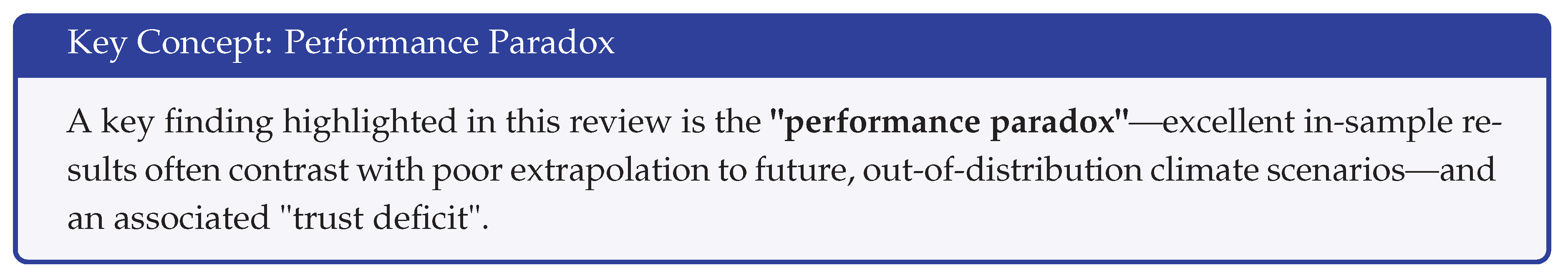
Throughout, we use performance paradox as the umbrella framing; where we say transferability crisis, we mean the same core phenomenon—poor out-of-distribution generalization under non-stationarity driven by covariate and concept drift.
2. Scope and Approach
This article is a narrative synthesis of recent research at the intersection of machine learning for climate and downscaling. Our goal is to distill design patterns, recurring pitfalls, and practical considerations rather than to provide an exhaustive catalogue. We focused on peer-reviewed work and influential preprints in climate, hydrology, and machine learning venues from 2010 to 2025, emphasizing studies that report transparent evaluation and are frequently referenced by the community. Coverage is selective and representative; when multiple papers make closely related contributions, we prioritize those with clearer methods, public code/data, or broader impact. Where appropriate, we group findings thematically and highlight open problems and promising directions.
3. Background: The Downscaling Problem
3.1. The Scale Gap in Climate Modeling and the Need for Downscaling
Global Climate Models (GCMs) serve as fundamental instruments for comprehending and forecasting climate change. However, their inherent coarse spatial resolution, typically ranging from 50 to 300 kilometers, presents a significant limitation for assessing climate change impacts at regional and local scales. This resolution is often inadequate for informing decisions in critical sectors such as agriculture, hydrology, energy resource management, urban planning, and disaster risk preparedness, all of which necessitate detailed, high-resolution climate information [4,8]. Downscaling techniques are therefore essential to bridge this "scale gap"—a challenge long recognized in climate science— transforming coarse GCM outputs into finer-scale climate projections that are relevant for localized impact studies and adaptation planning. The fundamental driver for the increasing adoption of machine learning (ML) in this domain is precisely this critical need for high-resolution climate data that GCMs cannot directly furnish, coupled with the inherent limitations of pre-ML downscaling methodologies.
3.2. Limitations of Traditional Downscaling Methods
Historically, two primary approaches have been employed for climate downscaling: dynamical downscaling and statistical downscaling.
3.2.1. Dynamical Downscaling (DD)
Dynamical Downscaling (DD) utilizes Regional Climate Models (RCMs), which are physics-based models run at higher resolutions over a limited area, driven by boundary conditions from GCMs. While DD provides physically consistent high-resolution outputs, it is exceptionally computationally intensive. For instance, the computational budget to simulate the global climate at 100 km resolution would be insufficient to dynamically downscale a region the size of Spain to 10 km [9]. This high computational cost severely restricts its application for downscaling large ensembles of GCMs, multiple future scenarios, or extended time periods, which are necessary for comprehensive uncertainty assessment. By contrast, RCMs themselves can introduce their own systematic biases [10].
3.2.2. Statistical Downscaling (SD)
Statistical Downscaling (SD), in its traditional forms (e.g., regression models, weather generators, analog methods), establishes empirical relationships between large-scale GCM predictors and local-scale climate variables (predictands) [11]. These methods are computationally far less demanding than DD. However, they often depend on strong assumptions, most notably the stationarity assumption—the premise that the statistical relationships derived from historical data will remain valid under future, potentially very different, climate conditions. This assumption is increasingly challenged by the non-stationary nature of climate change, a central theme explored in this review as it fundamentally impacts the reliability of ML models for future projections and is intrinsically linked to the concepts of covariate and concept drift discussed later (Section 8.3, Section 9.1, Section 7.4). Traditional SD methods may also struggle to capture complex non-linear interactions, spatial dependencies, and particularly the behavior of extreme climate events[4].
3.3. Emergence and Promise of ML in Transforming Statistical Downscaling
The advent of machine learning (ML), and deep learning (DL) in particular, has offered a powerful and flexible alternative to traditional SD methods [8]. ML models, especially DL architectures, possess the capability to learn highly complex, non-linear mappings between coarse-resolution predictor variables and fine-scale predictands directly from data. This data-driven approach allows for the automatic extraction of relevant features and relationships from large and diverse datasets, a characteristic that makes them particularly well-suited for tasks analogous to image super-resolution, which is conceptually similar to spatial downscaling [12]. The "deep learning revolution" in climate downscaling signifies more than just incremental improvements in performance metrics. It represents a fundamental shift in how the downscaling problem is approached: moving away from the explicit definition of statistical relationships (as in traditional SD) towards the learning of complex, often implicit, functions directly from observational or model-generated data. This paradigm shift offers immense potential for capturing intricate details and dependencies that were previously intractable. However, this increased power is accompanied by new and significant challenges, particularly concerning the interpretability of these "black-box" models and ensuring the physical consistency of their outputs. This review undertakes a critical examination of the advancements, capabilities, and persistent challenges associated with ML-based downscaling, focusing on the period between 2010 and 2025.
4. The Evolution of Machine Learning Approaches in Climate Downscaling
This section addressesRQ1by synthesizing how downscaling methods evolved from CNN/U/Net baselines to generative models (GANs, diffusion) and transformers/foundation models, including cross-resolution/region transfer and multi-task adaptation for downscaling [21,23,28,29,30,31].
To visually frame this critical analysis, we introduce a conceptual roadmap in Figure 1. This framework organizes the landscape of ML-based downscaling around the central challenge of the “performance paradox and trust deficit”—the tendency for models to show high skill on historical data but fail to generalize robustly, thereby limiting their operational trust. The roadmap connects this core problem to three primary axes of downscaling challenges: achieving high Spatial Fidelity, accurately representing Extreme Events, and ensuring robust Generalization & Uncertainty Quantification (UQ).
Each axis is mapped to the model families best suited to address it: CNNs and U-Nets for spatial structure, generative models like GANs and Diffusion for realism and extremes, and Transformers for generalization and long-term predictions. The figure further details the core strengths, inherent trade-offs, and key methodological innovations for each family, with the overarching goal of achieving Physical Consistency serving as a cross-cutting objective for the entire field. This layered framework will guide the subsequent sections as we delve into the evolution, challenges, and future trajectories of these technologies.
4.1. Early Applications and Classical ML Benchmarks
The application of machine learning to climate downscaling began with the exploration of classical ML algorithms, which served as important precursors to the current deep learning era. An early comprehensive intercomparison by Vandal et al. [32] benchmarked several statistical learning methods for daily and extreme precipitation downscaling, including Ordinary Least Squares (OLS), Elastic-Net, Support Vector Machines (SVM), Multi-task Sparse Structure Learning (MSSL), and autoencoders. Their findings indicated that for certain metrics and scenarios, simpler linear methods such as Bias Correction Spatial Disaggregation (BCSD) could consistently outperform more complex non-linear approaches. In practice, many agencies and impacts workflows still rely on well-tested statistical baselines—bias-corrected quantile mapping/BCSD and LOCA—so ML downscalers should be shown to surpass these incumbents on robust, application-relevant metrics [33,34,35].
This underscores an important consideration: the direct application of state-of-the-art machine learning does not always guarantee improvements over simpler, well-established statistical techniques, and classical models remain valuable for benchmarking. Support Vector Machines (SVMs) were among the early ML techniques applied, particularly for downscaling precipitation. For instance, Tripathi et al. [36] demonstrated the use of SVMs for downscaling precipitation in climate change scenarios. They have also reported promising results with SVMs, sometimes showing superior performance compared to Artificial Neural Networks (ANNs) for specific downscaling tasks. Random Forests (RFs) also found application, especially for precipitation downscaling, with some research indicating their utility in improving estimates of extreme precipitation events [37]. Further work has introduced specialized variants, such as a posteriori Random Forests (APRFs), which have proven effective at modeling the complete probability distribution of precipitation [38].
These initial studies were crucial in establishing the feasibility of using ML for downscaling. They highlighted that the success of these models often hinged on careful feature selection—identifying informative predictors—and was sensitive to the specific characteristics of the climate variable and the geographical region under study. Common hindrances included difficulties in adequately capturing complex spatiotemporal dependencies and the nuances of extreme events, limitations that paved the way for more sophisticated deep learning approaches. The rationale for choosing these classical models often stemmed from their established capabilities in general regression and classification tasks, their relative simplicity compared to the then-nascent deep learning models, and their greater interpretability.
Ghosh [39] combined SVMs with particle-swarm–guided simulated annealing for hyperparameter tuning in monsoon rainfall SD, showing early evidence that nonlinear ML can surpass linear baselines under multi-GCM uncertainty. Solved: robust nonparametric mapping under limited data. Open: explainability, extremes, and transfer to other regimes.
Quantile Regression Neural Networks Cannon [40] provided an early, practical probabilistic approach via direct quantiles, with left-censoring and bagging for calibration . Solved: distributional outputs and improved probability-of-precipitation. Open: quantile crossing; coupling across variables.
Prec-DWARF random forests He et al. [37] addressed heavy-rain underestimation with adaptive/paired forests, improving spatial patterns. Solved: stronger extremes in tree ensembles. Open: spatial coherence without CNN-like inductive bias.
Sequence models (2018–2019) including LSTM point-scale SD Misra et al. [41], CNN+LSTM hybrids for monsoon sequences [42], and regional LSTM SD for CMIP6 ensembles [43] improved persistence and multi-day events. Open: integration with spatial texture and physics.
Intercomparison Vandal et al. [1] showed strong linear/bias-correction methods remained competitive for daily and extreme indices, with early CNNs lagging. This frames the need for better losses, evaluation, and uncertainty.
4.2. The Deep Learning Paradigm Shift
The trajectory of ML in climate downscaling was significantly altered by the advent and rapid proliferation of deep learning techniques. This shift was largely inspired by the remarkable successes of DL in fields like computer vision, particularly in tasks such as image super-resolution, which bears conceptual resemblance to spatial climate downscaling [44].
4.2.1. Pioneering Work with Convolutional Neural Networks (CNNs)
DeepSD Vandal et al. [45] recast downscaling as image super-resolution using a stacked SRCNN pipeline that incrementally refines coarse ( 100 km) inputs to regional scales ( 12 km). The stacking strategy reduced error propagation versus a single large upsampling jump, and the multi-variate predictor set leveraged large-scale dynamics rather than only coarse precipitation. Challenge addressed: a scalable framework for multi-model ensembles and future projections. Outstanding issues: MSE loses smooth texture and attenuates extremes; no explicit physical constraints; limited out-of-distribution analysis for warming scenarios. Cross-links: cite in Extremes (as a baseline that underestimates tails) and in Evaluation to motivate spectra-/structure-aware metrics beyond RMSE.
Configuration/intercomparison Bano-Medina et al. [13] systematically varied CNN depth, filters, and training setups against strong statistical baselines, finding that naïve CNNs do not automatically dominate. Challenge addressed: clarifies when/why CNNs add value (spatial structure, precipitation extremes). Outstanding: sensitivity to architecture/loss and domain shifts. Cross-links: use when arguing for robust validation and baseline choice.
Continental-scale suitability Bano-Medina et al. [46] extended CNN SD to continental domains for temperature/precipitation projections . Challenge addressed: feasibility at scale without local hand-engineering. Outstanding: mean-temperature gains were modest; motivates hybrid or physics-aware losses. Cross-links: Physical consistency section.
Residual SR for daily temperature and precipitation Wang et al. [47] used deep residual blocks to stabilize training and preserve high frequencies, reporting improved extremes relative to plain CNNs . Challenge addressed: vanishing-gradient/depth limitations; better tail fidelity. Outstanding: still deterministic; uncertainty left implicit. Cross-links: Uncertainty (need ensembles) and Transferability (residual features reused across regions).
Daily 1 km multivariate SD in complex terrain Quesada-Chacón et al. [15] built U-Net style models to generate multiple variables (precipitation, temperature, radiation, vapor pressure, wind) at 1 km to 2100. Challenge addressed: multivariate coherence at fine scale with open, reproducible pipelines. Outstanding: quantifying cross-variable physical constraints (e.g., energy/water balances). Cross-links: Physical consistency (multivariate coherence) and Impact uses.
Iberia CMIP6 downscaling Soares et al. [48] demonstrated a rigorous regional application across variables with careful train/validation splits and diagnostics. Challenge addressed: operationalizing deep-learning statistical downscaling (DL SD) in a multi–Earth System Model (ESM) context (i.e., consistent training/transfer across multiple ESM outputs).
Outstanding: out-of-distribution robustness under future extremes and transfer to distinct climates. Cross-links: Evaluation (dataset curation) and Non-stationarity.
Convolutional Neural Networks (CNNs) were among the first DL architectures to demonstrate substantial potential in climate downscaling, primarily due to their inherent ability to learn hierarchical spatial features from gridded data.
A seminal work by Vandal et al. [12] introduced "DeepSD," a model based on Super-Resolution CNNs (SRCNNs), to downscale precipitation fields. This study showcased significant improvements in Root Mean Square Error (RMSE) compared to traditional bicubic interpolation and other statistical methods, effectively demonstrating that CNNs could capture complex non-linear relationships between coarse- and fine-scale precipitation patterns.
Building on this, Bano-Medina et al. [11] conducted one of the first comprehensive intercomparisons of various DL architectures for downscaling temperature and precipitation across continental Europe. Their analysis, utilizing the VALUE (Validation and Intercomparison of Downscaling Methods for Climate Change Research) framework, revealed that CNNs consistently outperformed traditional Generalized Linear Models (GLMs).
This work highlighted the particular strengths of U-Net architectures, a specialized type of CNN, in preserving spatial structures and fine details in the downscaled fields [8]. Legasa et al. [29] is another example of a study that evaluates CNNs against other methods for precipitation downscaling.
The rationale in these works for adopting CNNs was compelling: their architectural components, such as convolutional layers that apply learnable filters, pooling layers for dimensionality reduction, and weight sharing, are exceptionally well-suited for processing grid-based climate data [11]. These features enable CNNs to automatically learn relevant spatial features and complex relationships from the input data without requiring explicit, manually engineered features.
However, early and relatively "plain" CNN architectures were not without their limitations. For instance, training very deep plain CNNs proved challenging due to issues like vanishing or exploding gradients and the "degradation" problem, where adding more layers could paradoxically decrease performance. These models also tended to overfit, especially when dealing with sparse data like extreme precipitation events, and their ability to accurately capture such extremes was often limited.
4.2.2. Architectural Innovations
The initial successes with basic CNNs spurred rapid innovation in DL architectures tailored for or adapted to climate downscaling, aiming to overcome earlier limitations and enhance performance.
U-Nets
The U-Net architecture, originally developed for biomedical image segmentation [49], has been effectively applied in climate downscaling, where its skip-connection design showed clear performance improvements over previous statistical downscaling benchmarks [8]. U-Nets are characterized by a symmetric encoder-decoder structure. The encoder path progressively downsamples the input, capturing broader contextual information, while the decoder path upsamples these features to reconstruct a high-resolution output. A key feature of U-Nets is the use of "skip connections" that concatenate feature maps from the encoder layers directly to corresponding layers in the decoder. These skip connections allow the network to reuse fine-grained spatial information from earlier layers, which is crucial for preserving sharp details and accurate localization in the downscaled fields [8]. Variants like U-Net++ [50] and attention-augmented U-Nets, such as U-Net_DCA (U-Net with Dual Cross-Attention) [51], have further refined this approach, showing strong performance in downscaling tasks like wind fields. The U-Net architecture has also been found effective for GCM bias correction tasks, for example, in correcting Sea Surface Temperature (SST) projections from the CNRM-CM6 model, where it outperformed several other methods [52].
Residual Networks (ResNets)
To address the challenges of training very deep neural networks, ResNets introduced the concept of "residual learning" [53]. Instead of learning a direct mapping, ResNet layers learn a residual mapping with reference to the layer inputs, facilitated by shortcut or skip connections that perform identity mapping and are added to the output of stacked layers. This formulation makes optimization easier and allows for the construction of significantly deeper networks without suffering from degradation or vanishing gradients. In climate downscaling, architectures like the Super-Resolution Deep Residual Network (SRDRN) developed by Wang et al. [14] have demonstrated the benefits of this approach. SRDRN incorporates numerous residual blocks and batch normalization layers, enabling it to effectively extract multi-level features from climate data. Moreover, the SRDRN study highlighted the importance of data augmentation techniques, particularly for imbalanced datasets like daily precipitation, to improve the representation of extreme events and mitigate overfitting. Other ResNet-based models, such as Very Deep Super-Resolution (VDSR) [54] and Enhanced Deep Super-Resolution (EDSR) [55], have also shown superior performance in image super-resolution, outperforming simpler SR-CNNs by leveraging deeper architectures and residual learning, which has inspired similar approaches for downscaling tasks like temperature.
Generative Adversarial Networks (GANs)
GANs represent a distinct class of generative models that have been increasingly applied to climate downscaling, particularly when the goal is to produce highly realistic and sharp high-resolution fields. A GAN framework typically consists of two neural networks: a generator that learns to produce synthetic high-resolution data from low-resolution input, and a discriminator that learns to distinguish between the generator’s fake samples and real high-resolution data. These two networks are trained in an adversarial manner.
- Strengths:
- GANs have shown promise for generating outputs with improved perceptual quality, sharp gradients, and in some cases better representation of fine-scale variability and heavy-tailed statistics compared to models trained solely with pixel-wise losses like Mean Squared Error (MSE) [32]. StyleGAN-family architectures achieve low Fréchet Inception Distance (FID) scores across large-scale benchmarks, highlighting their strength for perceptually realistic textures [56,57]. Conditional GANs (CGANs), such as MSG-GAN-SD by Accarino et al. [58], demonstrate direct applicability to downscaling by conditioning generation on low-resolution input. While some studies report more realistic precipitation or temperature fields using CGANs [59], consistent advantages in reproducing extremes remain preliminary and context-dependent.
- Limitations:
- GANs are notoriously challenging to train due to issues like mode collapse (where the generator produces limited varieties of samples) and training instability [32]. Evaluating GAN performance can also be difficult, as traditional pixel-wise metrics may not fully capture perceptual quality. Moreover, while GANs can produce visually appealing results, some studies suggest they might not always accurately capture the full statistical distribution of the high-resolution data, which is critical for scientific applications [19]. The extrapolation of GANs for downscaling precipitation extremes in warmer, future climates remains an active area of research and concern. A notable application of GAN-based frameworks is the Super-Resolution for Renewable Energy Resource Data with Climate Change Impacts (Sup3rCC) model developed by the National Renewable Energy Laboratory (NREL) [60]. Sup3rCC employs a generative machine learning approach, specifically leveraging GANs, to downscale Global Climate Model (GCM) data to produce 4-km hourly resolution fields for variables crucial to the energy sector, such as wind, solar irradiance, temperature, humidity, and pressure, for the contiguous United States under various climate change scenarios. The model learns realistic spatial and temporal attributes by training on NREL’s historical high-resolution datasets (e.g., National Solar Radiation Database, Wind Integration National Dataset Toolkit) and then injects this learned small-scale information into coarse GCM inputs. This methodology is designed to be computationally efficient compared to traditional dynamical downscaling while providing physically realistic high-resolution data tailored for studying climate change impacts on energy systems, renewable energy generation, and electricity demand. It’s important to note that Sup3rCC is designed to represent the historical climate and future climate scenarios, rather than specific historical weather events [60].
Generative trends (synthesis). Recent work converges on a few clear themes. (1) Stochastic realism and ensemble spread: stochastic GAN super-resolution improves small-scale realism and supports ensemble evaluation [16]. (2) Adversarial SR beyond precipitation: adversarial downscaling for wind/solar highlights realism–likelihood trade-offs and motivates spectra-aware diagnostics for non-precip variables [61]. (3) Hybrid pipelines for extremes: coupling bias correction with a generative stage strengthens heavy-tail behavior and uncertainty depiction [17]. (4) Tail-aware objectives: explicit intensity-aware losses reduce wet/dry and high-intensity biases while remaining interpretable [2]. (5) Joint spatio-temporal scaling and transfer: global models achieve km-scale and sub-hourly resolution with promising cross-region transfer and efficient ensembles [62]. Taken together, these results point toward multi-stage and hybrid generative systems that balance likelihood, realism, extremes, and transferability, complemented by reliability checks (e.g., intensity-aware likelihoods, power spectra) and perfect-model tests for structure and conservation compliance.
Diffusion Models
Since 2020, diffusion probabilistic models [31] have emerged as a highly promising generative modeling technique, often overtaking GANs in computer vision due to their ability to generate high-quality, diverse samples and their more stable training dynamics. These models learn to reverse a gradual noising process, starting from a simple noise distribution and iteratively refining it to generate a data sample [31]. This iterative process allows them to capture complex, high-dimensional distributions with high fidelity, making them exceptionally well-suited for generating realistic and physically plausible climate fields.
Key innovations and applications in downscaling include:
- Latent Diffusion Models (LDMs): To mitigate the high computational cost of operating in pixel space, LDMs, such as those explored by Tomasi et al. [18], perform the diffusion process in a compressed latent space [63]. This significantly reduces training and sampling costs. For downscaling, LDMs have demonstrated the ability to mimic kilometer-scale dynamical model outputs (e.g., COSMO-CLM simulations) with remarkable fidelity for variables like 2m temperature and 10m wind speed, outperforming U-Net and GAN baselines in spatial error, frequency distributions, and power spectra [18].
- Spatio-Temporal and Video Diffusion: Recognizing the temporal nature of climate data, models like Spatio-Temporal Video Diffusion (STVD) extend video generation techniques to precipitation downscaling [19]. These frameworks often use a two-step process: a deterministic module (e.g., a U-Net) provides an initial coarse prediction, and a conditional diffusion model learns to add the high-frequency residual details. In initial experiments, STVD was reported to outperform GANs in capturing accurate statistical distributions and fine-grained precipitation structures, particularly those influenced by topography.
- Hybrid Dynamical-Generative Downscaling: A state-of-the-art paradigm combines the strengths of physical models and generative AI. As proposed by Lopez-Gomez et al. [9], this approach uses a computationally cheap RCM to dynamically downscale ESM output to an intermediate resolution. A generative diffusion model then refines this output to the final target resolution. This hybrid method leverages the physical consistency and generalizability of the RCM and the sampling efficiency and textural fidelity of the diffusion model. This approach not only reduces computational costs by over 97% compared to full dynamical downscaling but also produces more accurate uncertainty bounds and better captures spectra and multivariate correlations than traditional statistical methods.
- Distributional Correction: To better capture extreme events, recent work has focused on aligning the generated distribution with the target distribution, particularly in the tails. Liu et al. [20] introduced a Wasserstein penalty into a score-based diffusion model to improve the representation of extreme precipitation, demonstrating more reliable calibration across intensities.
Strengths: Diffusion models excel at capturing complex, multimodal distributions, leading to more realistic and diverse samples. They offer stable training without the mode collapse issues common in GANs and are inherently probabilistic, making them well-suited for uncertainty quantification through ensemble generation. Recent studies report promising results for probabilistic generation and UQ, including frameworks designed to estimate epistemic uncertainty in ensembles [31,64]. While these developments are encouraging, their application to downscaling remains at an early stage, and systematic evidence of superiority over GANs or other generative approaches is still limited.
Limitations: The primary drawback is computational expense, particularly the slow iterative sampling process, although LDMs and efficient sampling schemes are actively mitigating this [18]. Their application to climate downscaling is still an emerging area, and the optimal methods for conditioning and ensuring physical consistency are topics of active research.
Spatiotemporal Models (LSTMs, ConvLSTMs, Transformers)
Resolution-agnostic transformer Curran et al. [21] reported cross-resolution generalization using a pretrained Earth-ViT, suggesting zero/low-shot potential across grids. Solved: reduced retraining burden across input resolutions. Open: handling sparse or uneven observational coverage; incorporating explicit physical inductive biases (e.g., conservation constraints, symmetry/equivariance, monotonicity, or PDE-informed losses).Cross-links: Transferability and Operationalization.
Full-domain vs. tiling Pérez et al. [65] compared transformer SR strategies, showing trade-offs between global attention (context) and memory, and documenting boundary artifacts under naïve tiling. Solved: practical guidance for large regions. Open: context windows for extremes, efficient attention. Cross-links: Evaluation (seam artifacts) and Scalability.
Transformer precipitation SD Yang et al. [66] delivered a practical architecture that improves fidelity at moderate compute. Solved: competitive alternative to CNNs for precip SD. Open: tail calibration vs. GAN/diffusion; physics. Cross-links: Extremes, Compute. Recognizing that many climate variables exhibit strong temporal dependencies, researchers have employed architectures designed for sequential data.
-
LSTMs/ConvLSTMs: Long Short-Term Memory (LSTM) networks [67], a type of Recurrent Neural Network (RNN), are designed to capture long-range temporal dependencies in sequential data. Convolutional LSTMs (ConvLSTMs) [68] extend LSTMs by replacing fully connected operations with convolutional operations, enabling them to process spatio-temporal data where inputs and states are 2D or 3D grids [68,69]. These models are particularly relevant for downscaling precipitation sequences or forecasting river runoff using atmospheric forcing.Strengths: Explicitly model temporal sequences and dependencies, crucial for variables with memory effects. Hybrid CNN-LSTM models can leverage the spatial feature extraction capabilities of CNNs and the temporal modeling strengths of LSTMs, often outperforming standalone models [69].Limitations: Standard LSTMs might struggle with very high-dimensional spatial inputs unless effectively combined with convolutional structures. Training these complex recurrent architectures can also be demanding. While ConvLSTMs are better suited for spatio-temporal data, their ability to capture very long-range spatial dependencies might be limited compared to other architectures like Transformers.
-
Transformers: Originally developed for natural language processing [70], Transformer architectures, particularly Vision Transformers (ViTs) [71] and their variants, are increasingly being adopted for climate science applications, including downscaling [22]. Their core mechanism, self-attention, allows the model to weigh the importance of all other locations in the input when making a prediction for a single location. This enables the modeling of global context and long-range spatial dependencies (i.e., teleconnections), a critical advantage over the local receptive fields of CNNs.Key innovations and applications in downscaling include:
- −
- Architectural Adaptations: Models like SwinIR (Swin Transformer for Image Restoration) and Uformer have been adapted from computer vision for downscaling temperature and wind speed, demonstrating superior performance over CNN baselines like U-Net [72]. For precipitation, PrecipFormer utilizes a window-based self-attention mechanism and multi-level processing to significantly reduce computational overhead while effectively capturing the localized and dynamic nature of rainfall [24].
- −
- Resolution-Agnostic and Zero-Shot Downscaling: A significant frontier is the development of models that can generalize across different resolutions without retraining. Curran et al. [21] demonstrated that a pretrained Earth Vision Transformer (EarthViT) could be trained to downscale from 50km to 25km and then successfully applied to a 3km resolution task in a zero-shot setting (i.e., without any fine-tuning on the new resolution). This capability is crucial for operational efficiency, as it avoids the costly process of retraining models for every new GCM or grid configuration [21]. Research comparing various architectures found that a Swin-Transformer-based approach combined with interpolation surprisingly outperformed neural operators in zero-shot downscaling tasks in terms of average error metrics [73].
- −
- Foundation Models: The power and scalability of the Transformer architecture have made it the backbone for emerging foundation models in weather and climate science. Models like FourCastNet [22], Prithvi-WxC [23], and ORBIT-2 [74] are pre-trained on massive climate datasets (e.g., decades of ERA5 reanalysis). While primarily designed for forecasting, their learned representations of Earth system dynamics make them promising candidates for downscaling via fine-tuning. This paradigm shifts the task from training a specialized model from scratch to adapting a large, pre-trained model, which may enhance transferability and reduce data requirements for specific downscaling tasks, though this remains an active area of research [23,75]. This paradigm shifts the task from training a specialized model from scratch to adapting a large, pre-trained model, which can enhance transferability and reduce data requirements for specific downscaling tasks.
Strengths: Transformers excel at modeling long-range spatial and temporal dependencies, a key physical aspect of the climate system. They show strong potential for transfer learning and zero-shot generalization, which could dramatically reduce the computational burden of downscaling large, multi-model ensembles. Recent benchmarks indicate that Transformer architectures can achieve competitive or superior performance in zero-shot generalization across resolutions compared to some neural operator approaches [21,73]. While these findings are promising, they represent early results rather than a settled state-of-the-art, and broader validation across datasets and variables will be necessary. ViTs and their adaptations like PrecipFormer [24] (which uses window-based self-attention and multi-level processing for efficiency) and EarthViT [21] have shown promise in capturing complex spatio-temporal patterns. They exhibit good potential for transferability, especially when combined with CNNs in hybrid architectures [28]. Foundation models built on Transformers, such as Prithvi WxC [23] and ORBIT-2 [74], are being developed for multi-task downscaling across various variables and geographies. FourCastNet[22], another transformer-based model, is a weather emulator designed to resolve and forecast high-resolution variables like surface wind speed and precipitation.Limitations: The primary challenge is the quadratic computational complexity of the self-attention mechanism ( where N is the number of input patches), which can be prohibitive for very high-resolution data. However, innovations like window-based attention (Swin, PrecipFormer) and other efficient attention mechanisms are actively addressing this bottleneck [24]. Practically, their data-hungry nature means they benefit most from large-scale pre-training, making foundation models a key pathway for their effective use.
The progression from classical ML to diverse and specialized DL architectures signifies a field actively seeking more powerful and nuanced tools. While early CNNs provided a significant leap, the subsequent development of U-Nets, ResNets, GANs, LSTMs/ConvLSTMs, and now Transformers and Diffusion Models, reflects an ongoing effort to tackle the multifaceted challenges of climate downscaling. Each architectural family brings unique strengths—spatial feature extraction, temporal modeling, generative realism, long-range dependency capture—but also specific limitations, such as training stability, computational cost, or interpretability. This evolution indicates a maturing understanding that no single architecture is universally optimal; instead, the choice is increasingly driven by the specific characteristics of the downscaling problem, including the target variable, desired output properties (e.g., physical consistency, extreme event accuracy), and available computational resources. This specialization, however, also introduces complexity in terms of systematic intercomparison and the establishment of universally applicable best practices, a challenge that the community is actively addressing through initiatives like the CORDEX ML Task Force [76]. The diverse capabilities and trade-offs of these architectural families are summarized in the comparative matrix in Figure 2. This matrix highlights a central theme of this review: no single model family is universally superior. Instead, the state-of-the-art is task-dependent, requiring a careful match between the model’s inherent strengths—such as a GAN’s ability to generate sharp textures or a Transformer’s capacity for zero-shot generalization—and the specific requirements of the downscaling problem at hand.
This complex evolution, which involves a critical trade-off between model power and interpretability, is visualized in the timeline in Figure 3. The figure illustrates how the progression of ML models has been mirrored by an evolution in the scientific problem formulation itself, leading to a "trust deficit" that the community is now actively working to address.
5. The Physical Frontier: Hybrid and Physics-Informed Downscaling
While deep learning models excel at learning complex statistical patterns, a major criticism is that purely data-driven approaches can produce outputs that are physically implausible or inconsistent, violating fundamental laws like the conservation of mass and energy [25]. This lack of physical grounding is a primary contributor to the "trust deficit" and can lead to catastrophic failures when models are required to extrapolate to out-of-distribution future climates where historical statistical relationships may no longer hold. In response, two critical and rapidly growing research frontiers have emerged: Physics-Informed Machine Learning (PIML) and hybrid modeling frameworks.
5.1. The Imperative for Physical Consistency
The need for physical consistency is not merely academic; it is essential for scientific credibility and reliable impact assessment. For example, a downscaling model that does not conserve water mass can produce unrealistic runoff projections in hydrological models. Similarly, thermodynamically inconsistent combinations of temperature and humidity could lead to flawed assessments of heat stress. As highlighted by multiple studies, embedding physical laws directly into the learning process serves as a powerful form of regularization, guiding the model towards solutions that are not only accurate on training data but are also more likely to generalize robustly to unseen conditions [25].
5.2. Architectural Integration of Physical Laws: PIML
Physics-Informed Neural Networks (PINNs) and related PIML techniques integrate domain knowledge in the form of physical laws directly into the model’s architecture or training process [26,78]. This is typically achieved through two main strategies:
- Soft Constraints
- This is the most common approach, where the standard data-fidelity loss term () is augmented with a physics-based penalty term () [78]. The total loss becomes , where is a weighting hyperparameter. is formulated as the residual of a governing differential equation (e.g., the continuity equation for mass conservation). By minimizing this residual across the domain, the network is encouraged, but not guaranteed, to find a physically consistent solution. This method is flexible and has been used to penalize violations of conservation laws [25] and to solve complex PDEs [26].A common example is enforcing mass conservation in precipitation downscaling. If x is the value of a single coarse-resolution input pixel and are the n corresponding high-resolution output pixels from the neural network, a soft constraint can be added to the loss function to penalize deviations from the conservation of mass. In other words, the sum of the smaller pixels cannot be larger than the value of the corresponding coarse pixel. The total loss, , becomes a weighted sum of the data fidelity term (e.g., Mean Squared Error, ) and a physics penalty term:where is a hyperparameter that controls the strength of the physical penalty. Minimizing this loss encourages, but does not guarantee, that the mean of the high-resolution patch matches the coarse-resolution value.
- Hard Constraints (Constrained Architectures)
-
This approach modifies the neural network architecture itself to strictly enforce physical laws by design. For example, Harder et al. [27] introduced specialized output layers that guarantee mass conservation by ensuring that the sum of the high-resolution output pixels equals the value of the coarse-resolution input pixel. Such methods provide an absolute guarantee of physical consistency for the constrained property, which can improve both performance and generalization. While more difficult to design and potentially less flexible than soft constraints, they represent a more robust method for embedding inviolable physical principles [27]. In contrast of soft consrtraints, a hard constraint enforces the physical law by design, often through a specialized, non-trainable output layer. Continuing the mass conservation example, let be the raw, unconstrained outputs from the final hidden layer of the network. A multiplicative constraint layer can be designed to produce the final, constrained outputs that are guaranteed to conserve mass:This layer rescales the raw outputs such that their sum is precisely equal to , thereby strictly enforcing the conservation law at every forward pass, without the need for a penalty term in the loss function.
5.3. Hybrid Frameworks: Merging Dynamical and Statistical Strengths
Hybrid models seek to combine the strengths of traditional physics-based dynamical models (RCMs) with the efficiency and pattern-recognition capabilities of ML. Instead of replacing the physics entirely, ML is used to augment or accelerate parts of the physical modeling chain.
A state-of-the-art example is the dynamical-generative downscaling framework proposed by Lopez-Gomez et al. [9]. This multi-stage approach involves:
- An initial, computationally inexpensive dynamical downscaling step using an RCM to bring coarse ESM output to an intermediate resolution (e.g., from 100km to 45km). This step grounds the output in a physically consistent dynamical state.
- A subsequent generative ML step, using a conditional diffusion model, to perform the final super-resolution to the target scale (e.g., from 45km to 9km). The diffusion model learns to add realistic, high-frequency spatial details.
This hybrid strategy is powerful because it leverages the RCM for what it does best—ensuring physical consistency and generalization across different GCMs—while using the diffusion model for its strengths: computational efficiency and generating high-fidelity, stochastic textures. This approach was shown to reduce the computational cost of the most expensive downscaling stage by over 97.5% while producing outputs with lower errors and more realistic spatial spectra than traditional statistical methods [9]. Such hybrid frameworks represent a pragmatic and powerful path toward scalable, physically credible, and computationally tractable downscaling of large climate model ensembles.
5.4. Enforcing Physical Realism in Practice
5.4.1. The Frontier of Physics-Informed Machine Learning (PIML)
Physics-Informed Machine Learning (PIML) represents a burgeoning field that seeks to integrate physical knowledge directly into ML models, aiming to enhance their accuracy, generalizability, and physical consistency. This is particularly relevant for climate downscaling, where ensuring that outputs adhere to fundamental physical laws is critical for their credibility and utility.
The Promise of Physics-ML Integration
As highlighted by Harder et al. [27] and other studies [25], incorporating physical constraints directly into neural network training can yield significant benefits:
- Ensuring Conservation Laws: Models can be designed or constrained to conserve fundamental quantities like mass and energy [8].
- Maintaining Thermodynamic Consistency: Predictions can be guided to adhere to known thermodynamic relationships (e.g., between temperature, humidity, and precipitation).
- Reducing Data Requirements: By embedding prior physical knowledge, PIML models may require less training data to achieve good performance compared to purely data-driven approaches, as the physical laws provide strong regularization [26].
- Improving Extrapolation: Models that respect physical principles are hypothesized to extrapolate more reliably to unseen conditions, as these principles are expected to hold even when statistical relationships change.
Implementation Approaches for PIML
-
Hard Constraints: This approach involves modifying the neural network architecture or adding specific constraint layers at the output to strictly guarantee that certain physical laws are satisfied [27]. For example, a constraint layer could ensure that the total precipitation over a downscaled region matches the coarse-grid precipitation input, thereby enforcing water mass conservation.Advantages: Guarantees physical consistency for the enforced laws.Disadvantages: Can be more challenging to design and may limit the model’s flexibility if the constraints are too restrictive or incorrectly formulated.
-
Soft Constraints via Loss Functions: This is the more common approach, where penalty terms representing deviations from physical laws are added to the overall loss function that the model minimizes during training [26].Advantages: More flexible than hard constraints and can potentially incorporate multiple physical principles simultaneously. Easier to implement for complex, non-linear PDEs.Disadvantages: Does not strictly guarantee constraint satisfaction, only encourages it. The choice of weighting for the physics-based loss term () can be critical and may require careful tuning.
- Hybrid Statistical–Dynamical Models: As discussed previously, these models combine ML with components of traditional dynamical models [8]. ML can be used to emulate specific, computationally expensive parameterizations within an RCM, or to learn corrective terms for RCM biases. This approach inherently leverages the physical basis of the dynamical model components.
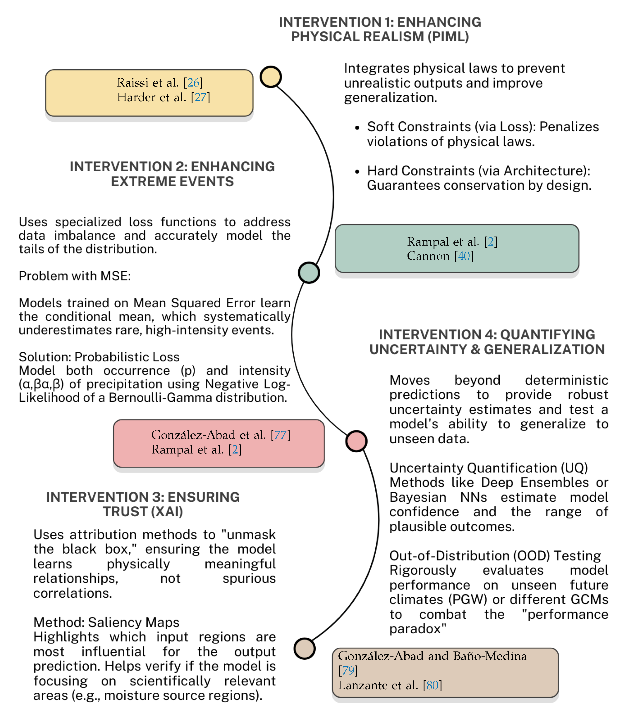
Figure 4.
A schematic of the primary methodological interventions to address the common failures of a standard ML downscaling pipeline. To overcome the “trust deficit,” researchers employ techniques to (1) enforce physical realism using PIML, (2) enhance extreme event representation with specialized loss functions, (3) ensure trust and scientific validity through XAI, and (4) robustly quantify uncertainty and test for out-of-distribution generalization.
Case Studies and Results
The application of PIML techniques in climate downscaling is an active area of research, with emerging studies demonstrating their potential. Emerging studies and conceptual analyses present a conceptual comparison showing that physics-informed DL can lead to improvements in RMSE, extreme event capture, energy conservation, and transferability compared to standard DL. For instance, Harder et al. [27] showed that their hard-constrained methods not only enforced conservation but also improved predictive performance on various climate datasets. Similarly, physics-informed loss functions are being developed to improve the representation of extreme events and other physical properties [81]. The integration of physical principles into ML models holds considerable promise for overcoming some of the key limitations of purely data-driven downscaling. By guiding the learning process with established physical knowledge, PIML approaches aim to produce downscaled climate information that is not only statistically skillful but also scientifically sound and reliable for understanding and adapting to climate change. However, the development of robust, generalizable, and computationally efficient PIML methods for the complex, multi-scale dynamics of the climate system remains a significant research challenge. While PIML offers a compelling pathway to more physically robust models, its operationalization in complex climate downscaling contexts is not without practical hurdles. The training process for PIML models can be significantly more computationally expensive than standard data-driven counterparts, particularly if involves calculating residuals of complex partial differential equations at numerous spatio-temporal points within each optimization iteration [82]. Scaling PIML to the multi-physics, multi-scale nature of climate systems is non-trivial. The crucial weighting factor in Equation 3 often requires careful, problem-specific tuning, potentially involving extensive hyperparameter searches, which can be an arduous task. Furthermore, formulating accurate and computationally tractable physical constraints for all relevant atmospheric processes in downscaling (e.g., cloud microphysics, radiative transfer, boundary layer dynamics) can be exceedingly difficult. Hard constraints, while guaranteeing adherence to enforced laws like mass conservation (e.g., Harder et al. [27]), can be architecturally complex to implement for phenomena beyond simpler conservation principles. These challenges underscore important avenues for future research, including developing more efficient PIML training algorithms, methods for automatically learning or discovering relevant physical constraints, or robust techniques for tuning .
The preceding sections traced how architectures evolved and how hybrid physics-ML designs aim to restore physical credibility without sacrificing statistical skill. However, across this diversity of models, inconsistent evaluation remains a primary obstacle to cumulative progress. Datasets, metrics, event definitions, and splits are rarely aligned, which hinders fair comparisons and obscures failure modes (e.g., non-stationarity, extremes, process-level errors). To address this, the next section proposes a prescriptive, model-agnostic evaluation protocol—spanning data splits, baseline anchors, event-focused metrics, physical diagnostics, and uncertainty tests—so results are both comparable and decision-relevant
6. Data, Variables, and Preprocessing Strategies in ML-Based Downscaling
The efficacy of any ML-based downscaling approach is profoundly influenced by the quality, characteristics, and processing of the input and target datasets, as well as the choice of variables. The selection of appropriate data sources and preprocessing strategies is crucial for training robust models that can generalize effectively.
6.1. Common Predictor Datasets (Low-Resolution Inputs)
The primary sources of low-resolution predictor data for ML downscaling models include global reanalysis products and outputs from GCMs and RCMs.
- ERA5 Reanalysis:
- The fifth generation ECMWF atmospheric reanalysis, ERA5, is extensively used as a source of predictor variables, particularly for training models in a "perfect-prognosis" framework [83,84]. ERA5 provides a globally complete and consistent, high-resolution (relative to GCMs, typically 31 km or 0.25°) gridded dataset of many atmospheric, land-surface, and oceanic variables from 1940 onwards, assimilating a vast amount of historical observations. Its physical consistency and observational constraint make it an ideal training ground for ML models to learn relationships between large-scale atmospheric states and local climate variables. Often, models trained on ERA5 are subsequently applied to downscale GCM projections.
- CMIP5/CMIP6 GCM Outputs:
- Outputs from the Coupled Model Intercomparison Project Phase 5 (CMIP5) and Phase 6 (CMIP6) GCMs are indispensable when the objective is to downscale future climate projections under various emission scenarios (e.g., Representative Concentration Pathways - RCPs, or Shared Socioeconomic Pathways - SSPs). These GCMs provide the large-scale atmospheric forcing necessary for projecting future climate change. However, their coarse resolution and inherent biases necessitate downscaling and often bias correction before their outputs can be used for regional impact studies [10,84].
- CORDEX RCM Outputs:
- Data from the Coordinated Regional Climate Downscaling Experiment (CORDEX) are also utilized, particularly when ML techniques are employed for further statistical refinement of RCM outputs, as RCM emulators, or in hybrid downscaling approaches. CORDEX provides dynamically downscaled climate projections over various global domains, offering higher resolution than GCMs and incorporating regional climate dynamics. However, these outputs may still require further downscaling for very local applications or may possess biases that ML can help correct.
6.2. High-Resolution Reference Datasets (Target Data)
The selection of high-resolution reference data, or "ground truth," is critical for training and validating supervised ML downscaling models.
- Gridded Observational Datasets:
- Products like PRISM (Parameter-elevation Regressions on Independent Slopes Model) for North America [8,85], Iberia01 for the Iberian Peninsula [86], E-OBS for Europe [87], and regional datasets like REKIS [88] are commonly used [8]. PRISM, for example, provides high-resolution (e.g., 800m or 4km) daily temperature and precipitation data across the conterminous United States, incorporating physiographic influences like elevation and coastal proximity into its interpolation [85]. These datasets are invaluable for training models in a perfect-prognosis setup, where historical observations are used as the target.
- Satellite-Derived Products:
- Satellite observations offer global or near-global coverage and are increasingly used as reference data. Notable examples include the Global Precipitation Measurement (GPM) mission’s Integrated Multi-satellitE Retrievals for GPM (IMERG) products for precipitation [89] and the Soil Moisture Active Passive (SMAP) mission for soil moisture [90]. GPM IMERG, for instance, provides precipitation estimates at resolutions like 0.1° and 30-minute intervals, with various products (Early, Late, and Final Run) catering to different latency and accuracy requirements [89].
- Regional Reanalyses or High-Resolution Simulations:
- In some cases, outputs from high-resolution regional reanalyses or dedicated RCM simulations (sometimes run specifically for the purpose of generating training data) are used as the "truth" data, especially when high-quality gridded observations are scarce [29].
- FluxNet:
- For variables related to land surface processes and evapotranspiration, data from the FluxNet network of eddy covariance towers provide valuable site-level observational data for model validation [91]. These towers measure exchanges of carbon dioxide, water vapor, and energy between ecosystems and the atmosphere.
The choice between these predictor and target datasets is contingent on the specific downscaling objective (e.g., future projections versus historical analysis), data availability for the region of interest, and the variables being downscaled. While ERA5 and CMIP6 GCMs are standard choices for predictor data, the target data often comes from gridded observations or specialized high-resolution model runs.
6.3. Key Downscaled Variables
The primary focus of ML-based downscaling has historically been on:
- Daily Precipitation and 2-meter Temperature: These are the most commonly downscaled variables due to their direct relevance for impact studies (e.g., agriculture, hydrology, health). This includes mean, minimum, and maximum temperatures.
- Multivariate Downscaling: There is a growing trend towards downscaling multiple climate variables simultaneously (e.g., temperature, precipitation, wind speed, solar radiation, humidity). This is important for ensuring physical consistency among the downscaled variables.
- Spatial/Temporal Scales: Typical downscaling efforts aim to increase resolution from GCM/Reanalysis scales of 25-100 km to target resolutions of 1-10 km, predominantly at a daily temporal resolution.
6.4. Feature Engineering and Selection
The process of selecting and engineering input features is critical for the success of ML-based downscaling.
- Static Predictors:
- High-resolution static geographical features such as topography (including elevation, slope, and aspect), land cover type, soil properties, and climatological averages are frequently incorporated as additional predictor variables. These features provide crucial local context that is often unresolved in coarse-scale GCM or reanalysis outputs. For instance, orography heavily influences local precipitation patterns and temperature lapse rates, while land cover affects surface energy balance and evapotranspiration [44,85]. The inclusion of these static predictors allows ML models to learn how large-scale atmospheric conditions interact with local surface characteristics to produce fine-scale climate variations.
- Dynamic Predictors:
- For specific variables like soil moisture, dynamic predictors such as Land Surface Temperature (LST) and Vegetation Indices (e.g., NDVI, EVI) derived from satellite remote sensing are often used, as these variables capture short-term fluctuations related to surface energy and water balance [92].
- Dimensionality Reduction and Collinearity:
- When dealing with a large number of potential predictors, dimensionality reduction techniques like Principal Component Analysis (PCA) are sometimes employed to reduce the number of input features while retaining most of the variance. This can help to mitigate issues related to collinearity among predictors and reduce computational load. Regularization techniques (e.g., L1 or L2 regularization) embedded within many ML models also implicitly handle collinearity by penalizing large model weights.
The careful selection and engineering of features, particularly the integration of high-resolution static geographical information, significantly enhances the ability of ML models to capture local climate nuances. This suggests that the models are not merely learning statistical correlations from atmospheric variables alone but are also learning the complex interactions between these variables and fixed surface characteristics.
6.5. Data Preprocessing Challenges
Several challenges related to data preprocessing must be addressed to ensure the development of robust and reliable ML downscaling models.
- Data-Scarce Areas: A significant hurdle is the availability of sufficient high-quality, high-resolution reference data for training and validation, especially in many parts of the developing world or in regions with complex terrain where observational networks are sparse [93].
- Imbalanced Data for Extreme Events: Extreme climatic events (e.g., heavy precipitation, heatwaves) are, by definition, rare. This leads to imbalanced datasets where extreme values are underrepresented, potentially biasing ML models (trained with standard loss functions like MSE) to perform well on common conditions but poorly on these critical, high-impact events. This issue often hinders models from learning the specific characteristics of extremes.
- Ensuring Domain Consistency: Predictor variables derived from GCM simulations may exhibit different statistical properties (e.g., means, variances, distributions) and systematic biases compared to reanalysis data (like ERA5) often used for model training. This mismatch, known as a domain or covariate shift, can degrade model performance and is a critical preprocessing consideration. This occurs because GCMs often have systematic biases and different statistical properties than reanalysis data, even for historical periods, thereby violating the assumption that training and application data are drawn from the same distribution. Techniques such as bias correction of GCM predictors, working with anomalies by removing climatological means from both predictor and predictand data to focus on changes, or more advanced domain adaptation methods are employed to mitigate this critical issue and enhance consistency [94].
- Quality Control and Gap-Filling: Observational and satellite-derived datasets frequently require substantial preprocessing steps, including quality control to remove erroneous data, and gap-filling techniques (e.g., interpolation) to handle missing values due to sensor malfunction or environmental conditions (like cloud cover for satellite imagery) [95].
The pervasive challenge of data imbalance for extreme events underscores a potential disconnect between generic ML advancements and the specific needs of climate science. Standard ML training objectives are often insufficient for applications where accurately capturing extremes is paramount, necessitating domain-specific adaptations in model architecture, loss functions, or data handling strategies.
7. A Prescriptive Protocol for Model Evaluation
To move beyond inconsistent evaluation practices and facilitate robust model intercomparison, this section outlines a prescriptive, multi-faceted evaluation protocol. A model’s true utility is not captured by a single metric; therefore, we propose a minimum viable suite of diagnostics tailored to the variable being downscaled, focusing on spatial structure, extreme events, and probabilistic skill. Adherence to such a protocol is a prerequisite for establishing the operational readiness of any ML downscaling method.
7.1. Protocol for Precipitation Downscaling
Precipitation is characterized by its intermittency, skewed distribution, and complex spatial structure. Evaluation must therefore prioritize metrics sensitive to these features over simple pixel-wise errors.
Recommended Minimum Suite:
- Root Mean Squared Error (RMSE): Report as a baseline metric for average error, but acknowledge its limitations in penalizing realistic high-frequency variability.
- Fraction Skill Score (FSS): This is the primary metric [96] for spatial accuracy. FSS should be reported for multiple intensity thresholds and spatial scales to assess performance across different event types. Based on common practice in forecast verification, we recommend thresholds relevant to hydrological impacts depending on usual severity of precipitation in that area and return period, for instance 1, 5, and 20 mm/day. The analysis should show FSS as a function of neighborhood size, with recommended spatial scales of the area in hand. We can take 10, 20, 40, and 80 km as an example; however, these values need to be carefully chosen to identify the scale at which the forecast becomes skillful.
- High-Quantile Error: To specifically evaluate performance on extremes, report the bias or absolute error for a high quantile of the daily precipitation distribution, such as the 99th or 99.5th percentile. This directly measures the model’s ability to capture the magnitude of rare, intense events.
- Power Spectral Density (PSD): Plot the 1D radially-averaged power spectrum of the downscaled precipitation fields against the reference data. This is a critical diagnostic for spatial realism. An overly steep slope indicates excessive smoothing, while a shallow slope or bumps at high frequencies can indicate unrealistic noise or GAN-induced artifacts.
- Continuous Ranked Probability Score (CRPS): For probabilistic models (e.g., GAN or Diffusion ensembles), the CRPS [97] is the gold-standard metric for overall skill, as it evaluates the entire predictive distribution. It should be reported as the primary probabilistic skill score.
7.2. Protocol for Temperature Downscaling
Surface temperature is a smoother, more continuous field than precipitation, but its evaluation still requires assessing distributional properties, bias, and, for probabilistic models, calibration.
Recommended Minimum Suite:
- RMSE and Bias: Report the overall Root Mean Squared Error and Mean Bias (downscaled minus reference) as standard metrics of accuracy and systematic error.
- Power Spectral Density (PSD): As with precipitation, the PSD is crucial for ensuring that the downscaled temperature fields contain realistic spatial variability and are not overly smoothed by the model.
- Distributional Metrics (e.g., Wasserstein Distance): Compare the full probability distributions of downscaled and reference temperatures using a robust metric like the Wasserstein Distance. This provides a more complete picture of performance than just comparing means and variances, capturing shifts in the shape and tails of the distribution.
- Reliability Diagram (for probabilistic models): If the model produces probabilistic forecasts (e.g., ensembles), a reliability diagram is essential. It plots the observed frequency of an event against the forecast probability, providing a direct visual assessment of calibration. A well-calibrated model should lie along the 1:1 diagonal line.
By adopting these variable-specific protocols, researchers can provide a much richer and more comparable assessment of model performance, moving the field towards a more rigorous standard of evaluation.
7.3. Comparative Analysis and State-of-the-Art
No single architecture is universally superior; the state-of-the-art is task-dependent:
- For spatial structure and deterministic accuracy, U-Net and ResNet-based CNNs remain strong contenders, particularly for smoother variables like temperature. Their inductive bias for local patterns is highly effective for learning topographically-induced climate variations [8].
- For probabilistic outputs and UQ, Diffusion models are emerging as the state-of-the-art due to their stable training and ability to generate high-fidelity, diverse ensembles [9,18]. They often outperform GANs on distributional metrics. As a simple, strong baseline for epistemic uncertainty, report deep ensembles [99] with CRPS and reliability diagnostics.
- For transferability and zero-shot generalization, Transformer-based foundation models represent the cutting edge. Their ability to learn from vast, diverse datasets enables generalization to new resolutions and regions with minimal fine-tuning, a critical capability for operational scalability [21].
7.4. Validation Under Non-Stationarity
The efficacy of statistical downscaling, including ML-based approaches, is fundamentally challenged by the non-stationary nature of the climate system under anthropogenic forcing. Relationships learned from historical data may not hold in a future, warmer world with altered atmospheric dynamics and potentially novel climate states. This section explores methodological innovations aimed at addressing non-stationarity and enhancing the physical realism of ML-downscaled projections.
The core assumption of many traditional statistical methods—that the statistical links between large-scale predictors and local-scale predictands remain constant over time—is increasingly untenable under rapid climate change. As articulated by Lanzante et al. [80], the relationships between large-scale and local-scale climate learned from historical data may not hold in a warmer world with altered atmospheric dynamics.
As discussed in subSection 8.3, this non-stationarity manifests as near-certain covariate and concept drift when projecting into the future. Models trained on historical data, which implicitly assume stationarity, are learning relationships specific to that historical period’s and . When future or change, the model’s performance degrades, forming a fundamental basis for the “transferability crisis”. This necessitates a shift towards methods that can either adapt to changing relationships or are inherently more robust to such shifts. We treat non-stationarity as a time-evolving distributional shift (a specific class of OOD input), typically manifesting as covariate and concept drift.
7.4.1. Pseudo-Global Warming (PGW) Experiments
PGW experiments involve modifying historical meteorological data to reflect conditions anticipated under future global warming scenarios, typically by adding climate change signals (e.g., temperature anomalies, changes in humidity) derived from GCM projections to observed historical weather patterns. ML models can then be trained or evaluated on these PGW datasets. This approach allows for a systematic assessment of a model’s ability to extrapolate to conditions outside its original training range but within a physically plausible future state. Studies employing PGW have shown potential improvements by exposing models to conditions more representative of future climates during training or testing.
7.4.2. Transfer Learning and Domain Adaptation
These techniques aim to leverage knowledge gained from one task or dataset (source domain) to improve performance on a different but related task or dataset (target domain) [8]. In the context of downscaling:
- Models might be pre-trained on large, diverse datasets (e.g., multiple GCMs, long historical records) to learn general, invariant features of atmospheric processes.
- These pre-trained models can then be fine-tuned on smaller, target-specific datasets (e.g., data for a particular region, a specific future period, or a new GCM) [28]. This approach can lead to better generalization and reduce the amount of target-specific data needed for training. However, careful validation is crucial to ensure that the transferred knowledge is beneficial and does not introduce biases from the source domain. Prasad et al. [28] demonstrated that pre-training on diverse climate datasets can enhance zero-shot transferability for some downscaling tasks, but fine-tuning often remains necessary for optimal performance on distinct target domains like different GCM outputs.
7.4.3. Process-Informed Architectures and Predictor Selection
Instead of relying solely on statistical pattern recognition, this approach seeks to imbue ML models with some degree of physical understanding by:
- Encoding known physical relationships into the network architecture: This might involve designing specific layers or connections that mimic physical processes or constraints.
- Using physically-motivated predictor variables: Selecting input variables that have a clear and robust physical link to the predictand (e.g., thermodynamic variables like potential temperature, specific humidity, or large-scale circulation indices known to influence local weather) rather than relying on a large set of potentially collinear or causally weak predictors.
While promising for enhancing robustness to non-stationarity, the implementation of truly process-informed architectures is still an area of active research with limited widespread adoption to date.
7.4.4. Validation Strategies for Non-Stationary Conditions
Traditional validation methods, which typically involve splitting historical data into training and testing sets, are insufficient for assessing a model’s performance under future climate change where the underlying data distributions may shift significantly. More robust validation strategies are emerging:
- Perfect Model Framework (Pseudo-Reality Experiments): In this setup, output from a high-resolution GCM or RCM simulation is treated as the “perfect” truth [80]. Coarsened versions of this output are used to train the ML downscaling model, which then attempts to reconstruct the original high-resolution “truth”. This framework allows for testing the ML model’s ability to downscale under different climate states (e.g., historical vs. future periods from the same GCM/RCM), as the “truth” is known for all periods. This is crucial for evaluating extrapolation capabilities.
- Cross-GCM Validation: Models are trained on a subset of available GCMs and then tested on GCMs that were not included in the training set. This assesses the model’s ability to generalize to climate model outputs with different structural characteristics and biases.
- Temporal Extrapolation (Out-of-Sample Testing): Using the most recent portion of the historical record or specific periods with distinct climatic characteristics (e.g., the warmest historical years as proxies for future conditions) exclusively for testing, after training on earlier data [8]. This provides a more stringent test of generalization than random cross-validation.
- Process-Based Evaluation: Beyond statistical metrics, evaluating whether the downscaled outputs maintain plausible physical relationships between variables (e.g., temperature–precipitation scaling, wind–pressure relationships) and accurately represent key climate processes (e.g., diurnal cycles, seasonal transitions, extreme event characteristics) under different climate conditions. XAI techniques can play a role here in verifying if the model is relying on physically sound mechanisms.
The challenge of non-stationarity is perhaps the most fundamental issue confronting ML-based statistical downscaling. Addressing it requires moving beyond purely empirical pattern-matching towards models that either incorporate more physical understanding or are explicitly designed and validated for robustness to changing climatic conditions. Also, when applying these validation strategies for non-stationary conditions, it is crucial to reiterate the importance of accounting for the non-IID nature of climate data, as discussed in Section 9.5. For instance, when performing temporal extrapolation to assess robustness to non-stationarity, employing temporal blocked cross-validation is more appropriate than standard random cross-validation to prevent leakage of future information into the training process. Similarly, when using the Perfect Model Framework across different climate states (e.g., historical vs. future simulations), ensuring spatial independence in training and test splits within each period, through techniques like spatial blocking or LLO CV, is vital for a fair assessment of generalization under changed conditions. To clarify the roles of these different approaches, Figure 5 presents a validation strategy matrix. This matrix maps the most critical validation techniques to the specific challenges they are designed to overcome, from mitigating data leakage due to spatio-temporal autocorrelation to rigorously testing out-of-distribution (OOD) generalization under future climate scenarios. Adopting a combination of these strategies is essential for moving beyond simple in-sample metrics and building trust in the operational readiness of ML downscaling models.
7.5. A Multi-Faceted Toolkit for Model Evaluation
The choice of evaluation metrics implicitly defines the objectives of downscaling. An over-reliance on pixel-wise metrics like RMSE can lead to overly smooth fields that fail to capture the spatial variability and extreme events crucial for impact studies. We propose a holistic evaluation toolkit, summarized in Table 1, that assesses performance across multiple dimensions.
Uncertainty Baselines
7.6. Operational Relevance: Beyond Statistical Skill
A model’s utility for real-world deployment depends on practical considerations beyond its performance on a test set.
- Computational Cost: Dynamical downscaling is exceptionally expensive, limiting its use for large ensembles. ML offers a computationally cheaper alternative by orders of magnitude [9,112]. However, costs vary within ML: inference with CNNs is fast, while the iterative sampling of diffusion models is slower. Training large foundation models requires massive computational resources, but once trained, fine-tuning and inference can be efficient [23]. The hybrid dynamical-generative approach offers a compelling trade-off, drastically cutting the cost of the most expensive part of the physical simulation pipeline [9].
- Interpretability: As discussed in Section 9.2.2, the "black-box" nature of deep learning is a major barrier to operational trust. The ability to use XAI tools to verify that a model is learning physically meaningful relationships, rather than spurious "shortcuts," is crucial for deployment in high-stakes applications.
- Robustness and Generalization: The single most important factor for operational relevance is a model’s ability to generalize to out-of-distribution(OOD) data, namely future climate scenarios. As detailed in Section 9.1, models that fail under covariate or concept drift are not operationally viable for climate projection. Therefore, rigorous OOD evaluation using techniques like cross-GCM validation and Pseudo-Global Warming (PGW) experiments is a prerequisite for deployment.
- Baselines: Always include strong classical comparators (e.g., BCSD/quantile-mapping and LOCA) as default references alongside modern DL models; these remain common operational choices in hydrologic and climate-services pipelines [33,34]. Formal assessments and national products continue to operationalize statistical interfaces between GCMs and impacts—bias adjustment and empirical/statistical downscaling (e.g., LOCA2, STAR-ESDM)—as default pathways, which underscores why ML downscalers must demonstrate clear, application-relevant added value [113,114].
8. Critical Investigation of Model Performance and Rationale
A critical aspect of advancing ML-based downscaling involves understanding not only which models perform well, but why they do so, and conversely, what factors impede their learning and generalization capabilities. This requires a careful examination of the rationale behind model choices and a comparative analysis of their strengths and weaknesses in the context of specific downscaling tasks.
8.1. Rationale for Model Choices
The selection of a particular ML architecture for climate downscaling is often guided by the inherent strengths of the architecture in handling specific types of data and learning particular kinds of patterns.
- CNNs/U-Nets for Spatial Patterns:
- These architectures are predominantly chosen for their proficiency in learning hierarchical spatial features from gridded data. Convolutional layers are adept at identifying local patterns, while pooling layers capture broader contextual information. U-Nets, with their encoder-decoder structure and skip connections, are particularly favored for tasks requiring precise spatial localization and preservation of fine details, making them well-suited for downscaling variables like temperature and precipitation where spatial structure is paramount [8].
- LSTMs/ConvLSTMs for Temporal Dependencies:
- When the temporal evolution of climate variables and their sequential dependencies are critical (e.g., for daily precipitation sequences or hydrological runoff forecasting), LSTMs and ConvLSTMs are preferred due to their recurrent nature and ability to capture long-range temporal patterns.
- GANs/Diffusion Models for Realistic Outputs and Extremes:
- These generative models are selected when the objective is to produce downscaled fields that are not only statistically accurate but also perceptually realistic, with sharp gradients and a better representation of the full statistical distribution, including extreme events [8].
- Transformers for Long-Range Dependencies:
The selection process reflects an understanding that different climate variables possess distinct characteristics—for example, the relatively smooth spatial continuity of temperature versus the highly intermittent and patchy nature of precipitation. This distinction often guides the choice towards architectures whose inductive biases align with these characteristics.
8.2. Factors Contributing to Model Success
Several factors consistently contribute to the successful application of ML models in climate downscaling:
- Appropriate Architectural Design: Matching the model architecture to the inherent characteristics of the data and the downscaling task is paramount. For instance, CNNs are well-suited for gridded spatial data, while LSTMs excel with time series. The incorporation of architectural enhancements like residual connections and the skip connections characteristic of U-Nets have proven crucial for training deeper models and preserving fine-grained spatial detail.
- Effective Feature Engineering: The performance of ML models is significantly boosted by the inclusion of relevant predictor variables. In particular, incorporating high-resolution static geographical features such as topography, land cover, and soil type provides essential local context that coarse-resolution GCMs or reanalysis products inherently lack. This allows the model to learn how large-scale atmospheric conditions are modulated by local surface characteristics.
- Quality and Representativeness of Training Data: The availability of sufficient, high-quality, and representative training data is fundamental. Data augmentation techniques, such as rotation or flipping of input fields, can expand the training set and improve model generalization, especially for underrepresented phenomena like extreme events [14,115].
- Appropriate Loss Functions: The choice of loss function used during model training significantly influences the characteristics of the downscaled output. While standard loss functions like MSE are common, they can lead to overly smooth predictions and poor representation of extremes. Tailoring loss functions to the specific task—for example, using quantile loss, Bernoulli-Gamma loss for precipitation (which models occurrence and intensity separately), Dice loss for imbalanced data, or the adversarial loss in GANs for perceptual quality—can lead to substantial improvements in capturing critical aspects of the climate variable’s distribution [8]. Studies show that L1 and L2 loss functions perform differently depending on data balance, with L2 often being better for imbalanced data like precipitation [116].
- Rigorous Validation Frameworks: The use of robust validation strategies, including out-of-sample testing and standardized evaluation metrics beyond simple error scores (e.g., the VALUE framework [117]), is crucial for assessing true model skill and generalizability.
8.3. Factors Hindering Model Learning
Despite their successes, ML models can be hindered by several factors that impede their ability to learn effectively or generalize reliably:
- Overfitting: Models may learn noise or spurious correlations present in the specific training dataset, leading to excellent performance on seen data but poor generalization to unseen data. This is a common issue, especially with highly flexible DL models and limited or non-diverse training data.
-
Poor Generalization (The "Transferability Crisis"), Covariate Shift, Concept Drift, and Shortcut Learning: A major and persistent challenge is the failure of models to extrapolate reliably to conditions significantly different from those encountered during training. This ’transferability crisis’ is the core of the "performance paradox" and is rooted in the violation of the stationarity assumption. It can be rigorously framed using established machine learning concepts:
- −
- Covariate Shift: This occurs when the distribution of input data, , changes between training and deployment, while the underlying relationship remains the same [118]. In downscaling, this is guaranteed when applying a model trained on historical reanalysis (e.g., ERA5) to the outputs of a GCM, which has its own systematic biases and statistical properties. It also occurs when projecting into a future climate where the statistical distributions of atmospheric predictors (e.g., mean temperature, storm frequency) have shifted.
- −
- Concept Drift: This is a more fundamental challenge where the relationship between predictors and the target variable, , itself changes [118]. Under climate change, the physical processes linking large-scale drivers to local outcomes might be altered (e.g., changes in atmospheric stability could alter lapse rates). A mapping learned from historical data may therefore become invalid.
- −
- Shortcut Learning: This phenomenon provides a mechanism to explain why models are so vulnerable to these shifts [119]. Models often learn "shortcuts"—simple, non-robust decision rules that exploit spurious correlations in the training data instead of the true underlying physical mechanisms [119]. For example, a model might learn to associate a specific GCM’s known regional cold bias with a certain type of downscaled precipitation pattern. This shortcut works perfectly for that GCM but fails completely when applied to a different, unbiased GCM or to the real world, leading to poor OOD performance. The finding by González-Abad et al. [77] that models may rely on spurious teleconnections is a prime example of shortcut learning in this domain.
The difficulty in generalizing to these OOD conditions is therefore a core impediment. High performance on historical, in-distribution test data provides no guarantee of reliability for future projections, necessitating strategies focused on robustness, physical understanding, and OOD detection. - Lack of Physical Constraints: Purely data-driven ML models, optimized solely for statistical accuracy, can produce outputs that are physically implausible or inconsistent (e.g., violating conservation laws). This lack of physical grounding can severely limit the trustworthiness and utility of downscaled projections.
- Data Limitations: Insufficient training data, particularly for rare or extreme events, remains a significant bottleneck. Data scarcity in certain geographical regions also poses a challenge for developing globally applicable models. Furthermore, the lack of training data that adequately represents the full range of potential future climate states can hinder a model’s ability to project future changes accurately.
- Inappropriate Model Complexity: Choosing an inappropriate level of model complexity can be detrimental. Models that are too simple may underfit the data, failing to capture complex relationships. Conversely, overly complex models are prone to overfitting, may be more difficult to train, and can be computationally prohibitive.
- Training Difficulties (e.g., Vanishing/Exploding Gradients): In very deep neural networks, especially plain CNNs without architectural aids like residual connections, the gradients used for updating model weights can become infinitesimally small (vanishing) or excessively large (exploding), hindering the learning process.
- Input Data Biases and Inconsistencies: Systematic biases present in GCM outputs, or inconsistencies between the statistical characteristics of training data (e.g., reanalysis) and application data (e.g., GCM outputs from a different model or future period), representing a significant covariate shift as discussed previously, can significantly degrade downscaling performance. Preprocessing steps, such as bias correction of predictors or working with anomalies by removing climatology, are often crucial for mitigating these issues [80].
The difficulty in generalizing to out-of-sample conditions, often linked to models learning superficial statistical correlations rather than robust physical mechanisms, represents a core impediment. This suggests that high performance on historical test data does not automatically translate to reliability for future climate projections, necessitating specific strategies to enhance model robustness and physical understanding.
8.4. Comparative Analysis of ML Approaches
AI-assisted ERA5 precipitation learned a mapping from ERA5 atmospheric proxies (and satellite estimates) to high-resolution observed precipitation, effectively performing bias-correction and downscaling in one step [120]. Solved: a practical route to operational products with good transfer to unseen regions. Open: explicit uncertainty and physical conservation. A comparative understanding of different ML architectures is essential for selecting appropriate methods for specific downscaling tasks. Table 2 provides a synthesis of dominant ML architectures used in climate downscaling, outlining their key mechanisms, strengths, limitations, typical applications, and resolutions.
The development and application of these diverse architectures indicate that the field is moving towards more tailored solutions. The "best" model is not a fixed entity but depends on a nuanced understanding of the problem at hand—the specific climate variable, the geographical context, the importance of physical consistency versus perceptual realism, and the need to capture extreme events. This highlights a crucial understanding: model performance is an emergent property of the entire downscaling pipeline, encompassing not just the architecture but also the quality of input features, the appropriateness of the loss function, and the rigor of the validation strategy. A sophisticated architecture can falter if other components of this pipeline are suboptimal, particularly for challenging tasks like accurately downscaling extreme precipitation or ensuring physical consistency under future climate scenarios.
9. Overarching Challenges in ML-Based Climate Downscaling
Despite the significant advancements and demonstrated potential of machine learning in climate downscaling, several overarching challenges persist. These challenges often interrelate and collectively hinder the operational deployment and full realization of ML’s capabilities in providing robust and trustworthy high-resolution climate information. Key among these are issues of transferability and domain adaptation, ensuring physical consistency and interpretability, effectively representing extreme events, quantifying uncertainties, and addressing practical aspects like reproducibility and data limitations.
9.1. Transferability and Domain Adaptation: The Achilles’ Heel
One of the most critical and frequently cited limitations of ML-based downscaling methods, particularly for deep learning models, is their often poor transferability or generalizability to data distributions different from those on which they were trained [80]. Recent intercomparison studies, such as Legasa et al. [29], are now directly assessing the transferability of different ML methods (including CNNs and Random Forests) by comparing how well they preserve the climate change signals projected by the driving GCM [80]. The fundamental root cause of these transferability issues often lies in the violation of the stationarity assumption implicitly made by many ML models, compounded by the models learning statistical shortcuts instead of robust physical relationships. As discussed earlier (Section 8.3), these failures can be rigorously framed using the concepts of covariate shift and concept drift. Covariate shift, where the distribution of input predictors changes between training and application, is almost guaranteed when moving from historical data to future climate projections, or from reanalysis products to GCM outputs. For example, GCM projections for future climates will inevitably present different statistical distributions of large-scale atmospheric predictors (e.g., altered mean temperatures, changes in variability patterns) compared to the historical data used for training. Similarly, models trained on reanalysis data like ERA5 (as ) often encounter a covariate shift when applied to GCM outputs (), which possess systematic biases and distinct statistical properties even for the same historical period. This is closely related to the challenges of “Ensuring Domain Consistency” (Section 6.5) and “Input Data Biases and Inconsistencies” (Section 8.3).
Concept drift, a change in the underlying relationship between predictors and predictands, is also highly probable under climate change. The physical processes linking large-scale atmospheric drivers (X) to local climate variables (Y) might themselves evolve due to factors like altered atmospheric stability or land-surface feedbacks. Consequently, a mapping learned from historical data may cease to be optimal or even valid for future conditions. Furthermore, different GCMs, with their unique physical parameterizations, might inherently represent the relationship differently. Applying a downscaling model trained on one GCM’s representation of to another GCM could thus encounter concept drift, even if their large-scale predictors X were perfectly harmonized.
The “performance paradox”—where models achieve excellent performance on historical, in-distribution test sets but fail catastrophically when faced with these shifts—is a direct consequence of models encountering covariate and concept shifts without being robust to them, often because they have learned shortcuts valid only for the training distribution.
These models learn relationships ( and from ) specific to the historical period. When future changes (covariate shift) or future changes (concept drift), the model’s performance degrades. This provides a more fundamental explanation for the “transferability crisis” than merely stating models learn “statistical shortcuts”; they learn shortcuts that are only valid for the training distribution and are not robust to these inevitable distributional shifts. This "Achilles’ heel" manifests in several ways:
- Extrapolation to Future Climates: Models trained exclusively on historical climate data often struggle to perform reliably when applied to future climate scenarios characterized by significantly different mean states, altered atmospheric dynamics, or novel patterns of variability. Studies by Hernanz et al. [121] demonstrated catastrophic drops in CNN performance when applied to future projections or GCMs not included in the training set. The models may learn statistical relationships that are valid for the historical period but do not hold under substantial climate change.
- Cross-GCM/RCM Transfer: Due to inherent differences in model physics, parameterizations, resolutions, and systematic biases, ML models trained to downscale the output of one GCM or RCM often exhibit degraded performance when applied to outputs from other climate models. This limits the ability to readily apply a single trained downscaling model across a multi-model ensemble.
- Spatial Transferability: A model developed and trained for a specific geographical region may not transfer effectively to other regions with different climatological characteristics, topographic complexities, or land cover types. Local adaptations are often necessary, which can be data-intensive.
The fundamental root cause of these transferability issues often lies in the stationarity assumption implicitly made by many ML models. These models learn statistical correlations from the training data, and if these correlations are spurious or specific only to the training period’s climate regime, they will not generalize to non-stationary future conditions where the underlying physical relationships () may change.
Several mitigation efforts and active research frontiers are addressing this challenge:
- Domain Adaptation Techniques: These methods aim to explicitly adapt a model trained on a "source" domain (e.g., historical data from one GCM) to perform well on a "target" domain (e.g., future data from a different GCM) where labeled high-resolution data may be scarce or unavailable [8].
- Training on Diverse Data: A common strategy is to pre-train ML models on a wide array of data encompassing multiple GCMs, varied historical periods, and diverse geographical regions. The hypothesis is that exposure to greater variability will help the model learn more robust and invariant features that generalize better. For instance, Prasad et al. [28] found that training on diverse datasets (ERA5, MERRA2, NOAA CFSR) led to good zero-shot transferability for some tasks, though fine-tuning was still necessary for others, such as the two-simulation transfer involving NorESM data.
- Pseudo-Global Warming (PGW) Experiments: This approach involves training or evaluating models using historical data that has been perturbed to mimic certain aspects of future climate conditions (e.g., by adding a GCM-projected warming signal). This allows for a more systematic assessment of a model’s extrapolation capabilities under changed climatic states.
-
Causal Machine Learning: There is growing interest in developing ML approaches that aim to learn underlying causal physical processes rather than just statistical correlations. Such models are hypothesized to be inherently more robust to distributional shifts.The challenge of transferability implies that simply achieving high accuracy on a historical test set is insufficient. For ML-downscaled projections to be credible for future climate impact assessments, models must demonstrate robustness across different climate states and sources of climate model data.
Case Studies (Quantitative Case Studies)
- Cross-model transfer (temperature UNet emulator). In a pseudo-reality experiment, daily RMSE for a UNet emulator rose from ∼0.9°C when evaluated on the same driving model used for training (UPRCM) to ∼2–2.5°C when applied to unseen ESMs; for warm extremes (99th percentile) under future climate, biases were mostly within C but reached up to C in some locations, and were larger than a linear baseline [121].
- GAN downscaling artifacts (near-surface winds). Deterministic GAN super-resolution exhibited systematic low-variance (low-power) bias at fine scales and, under some partial frequency-separation settings, isolated high-power spikes at intermediate wavenumbers; allowing the adversarial loss to act across all frequencies restored fine-scale variance, but it also raised pixelwise errors via the double-penalty effect.” [98].
- Classical SD variability & bias pitfalls (VALUE intercomparison). In a 50+ method cross-validation over Europe, several linear-regression SD variants showed very large precipitation biases—sometimes worse than raw model outputs—while some MOS techniques systematically under- or over-estimated variability (e.g., ISI-MIP under, DBS over), underscoring that method class alone does not guarantee robustness [5].
9.2. Physical Consistency and Interpretability
Beyond statistical accuracy, two crucial aspects for the trustworthiness and scientific utility of ML-downscaled climate data are their physical consistency and the interpretability of the models that produce them.
9.2.1. Ensuring Physically Plausible Outputs
A significant concern with purely data-driven ML models is their potential to produce outputs that violate fundamental physical laws, such as the conservation of mass or energy, or exhibit thermodynamically inconsistent relationships between variables. For example, downscaled precipitation fields might not conserve water mass when aggregated back to the coarse scale, or predicted temperature and humidity fields might imply unrealistic atmospheric stability.
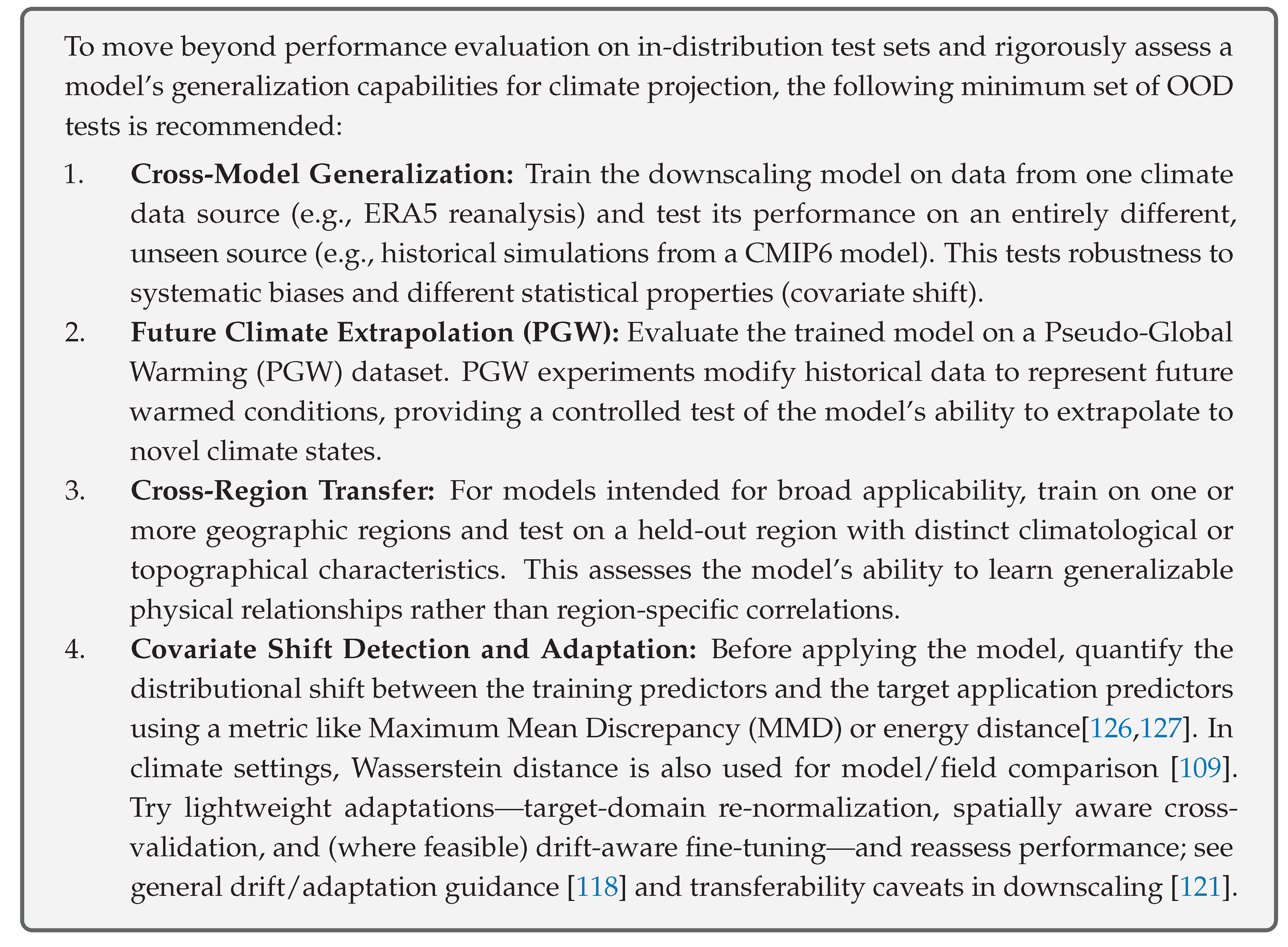
Within the body of work we surveyed, explicit enforcement of physical laws (e.g., conservation of mass or energy) is relatively uncommon compared to purely data-driven approaches. While we did not attempt to quantify this precisely, our reading of the literature indicates that physics-aware methods remain underrepresented. This lack of physical grounding can lead to scientifically questionable or misleading results, undermining confidence in ML-based downscaling. Efforts to address this challenge fall broadly into two categories:
-
Physics-Informed Neural Networks (PINNs) and Constrained Learning:
- −
- Soft Constraints: This approach involves incorporating penalty terms into the model’s loss function that discourage violations of known physical laws. The total loss becomes a weighted sum of a data-fidelity term and a physics-based regularization term (e.g., ). Physics-informed loss functions have been explored to guide models towards more physically realistic solutions. While soft constraints can reduce the frequency and magnitude of physical violations, they may not eliminate them entirely and can introduce a trade-off between statistical accuracy and physical consistency [25].
- −
- Hard Constraints: These methods aim to strictly enforce physical laws by design, either by modifying the neural network architecture itself or by adding specialized output layers that ensure the predictions satisfy the constraints. Harder et al. [27] introduced additive, multiplicative, and softmax-based constraint layers that can guarantee, for example, mass conservation between low-resolution inputs and high-resolution outputs. Such hard-constrained approaches have been shown to not only ensure physical consistency but also, in some cases, improve predictive performance and generalization [27]. The rationale for PINNs includes reducing the dependency on large datasets and enhancing model robustness by ensuring physical consistency, especially in data-sparse regions or for out-of-sample predictions [26]. Recent work explores Attention-Enhanced Quantum PINNs (AQ-PINNs) for climate modeling applications like fluid dynamics, aiming for improved accuracy and computational efficiency [128].
- Hybrid Dynamical-Statistical Models: Another avenue is to combine the strengths of ML with traditional physics-based dynamical models (RCMs). This can involve using ML to emulate computationally expensive components of RCMs, to statistically post-process RCM outputs (e.g., for bias correction or further downscaling), or to develop hybrid frameworks where ML and dynamical components interact [8,29]. For example, "dynamical-generative downscaling" approaches combine an initial stage of dynamical downscaling with an RCM to an intermediate resolution, followed by a generative AI model (like a diffusion model) to further refine the resolution to the target scale. This leverages the physical consistency of RCMs and the efficiency and generative capabilities of AI [9]. Such hybrid models aim to achieve a balance between computational feasibility, physical realism, and statistical skill.
The integration of physical knowledge, whether through soft or hard constraints or via hybrid modeling, is increasingly recognized as crucial for developing ML downscaling methods that are not only accurate but also scientifically credible and reliable for climate change applications.
9.2.2. Explainable AI (XAI): Unmasking the "Black Box"
Deep learning models are often criticized for being "black boxes" due to their complex internal workings, making it difficult to understand the reasoning behind their predictions [8]. In the context of climate science, where understanding underlying processes and building trust in model projections are paramount, this lack of transparency is a significant barrier. Explainable AI (XAI) techniques aim to shed light on how these models arrive at their decisions. We have observed that relatively few of the reviewed studies incorporate XAI.
9.2.2.1. The Need for Interpretability
XAI is crucial for several reasons:
- Model Validation and Debugging: Understanding which input features a model relies on can help identify if it has learned scientifically meaningful relationships or if it is exploiting spurious correlations or artifacts in the training data. Understanding which input features a model relies on can help identify if it has learned scientifically meaningful relationships or if it is exploiting spurious correlations or artifacts in the training data - a phenomenon of shortcut learning where models may appear "right for the wrong reasons".
- Scientific Discovery: XAI can potentially reveal novel insights into climate processes by highlighting unexpected relationships learned by the model.
- Building Trust: Transparent models whose decision-making processes align with physical understanding are more likely to be trusted by domain scientists and policymakers.
- Identifying Biases: XAI can help uncover hidden biases in the model or the data it was trained on.
9.2.2.2. Common XAI Techniques Applied to Downscaling
- Saliency Maps and Feature Attribution: Methods like Integrated Gradients, DeepLIFT, and Layer-Wise Relevance Propagation (LRP) aim to attribute the model’s output (e.g., a high-resolution pixel value) back to the input features (e.g., coarse-resolution predictor fields), highlighting which parts of the input were most influential [8]. González-Abad et al. [77] introduced aggregated saliency maps for CNN-based downscaling, revealing that models might rely on spurious teleconnections or ignore important physical predictors. LRP has been adapted for semantic segmentation tasks in climate science, like detecting tropical cyclones and atmospheric rivers, to investigate whether CNNs use physically plausible input patterns [129].
- Gradient-weighted Class Activation Mapping (Grad-CAM): This technique produces a coarse localization map highlighting the important regions in the input image for predicting a specific class (or, adapted for regression, a specific output value) [130]. While useful for visualization, Grad-CAM may not differentiate well between input variables [129].
- SHAP (SHapley Additive exPlanations): Based on cooperative game theory, SHAP values explain the prediction of an instance by computing the contribution of each feature to the prediction [131]. SHAP has been noted for its ability to reveal features that degrade forecast accuracy, though it may inaccurately rank significant features in some contexts [132].
9.2.2.3. Challenges in XAI for Climate Downscaling
- Faithfulness and Plausibility: Ensuring that explanations truly reflect the model’s internal decision-making process (faithfulness) and are consistent with physical understanding (plausibility) is challenging [133]. Different XAI methods can yield different, sometimes conflicting, explanations for the same prediction [134].
- Relating Attributions to Physical Processes: While methods like integrated gradients are mathematically sound, the resulting attribution maps can be difficult to directly relate to specific, understandable physical processes or mechanisms.
- Standardization: Methodologies and reporting standards for XAI in climate downscaling remain inconsistent, making comparisons across studies difficult. Different XAI methods can yield conflicting explanations for the same prediction, and there is a lack of consensus on benchmark metrics, hindering systematic evaluation [133].
- Beyond Post Hoc Explanations: Current XAI often provides post hoc explanations. There is a growing call to move towards building inherently interpretable models or to integrate interpretability considerations into the model design process itself, drawing lessons from how dynamical climate models are understood at a component level. This involves striving for "component-level understanding" where model behaviors can be attributed to specific architectural components or learned representations.
The development and integration of robust and meaningful XAI techniques are vital for transforming ML downscaling models from "black boxes" into transparent and trustworthy scientific tools.
9.3. Representation of Extreme Events
Climate extremes, such as heavy precipitation, droughts, heatwaves, and cold spells, often have the most significant societal and environmental impacts. Therefore, the ability of downscaling methods to accurately represent the characteristics of these extreme events (e.g., frequency, intensity, duration, spatial extent) is of paramount importance [44].
The Challenge
Standard ML models, particularly those trained with common loss functions like MSE, tend to perform poorly in capturing extreme events. This is often because:
- Data Imbalance: Extreme events are rare by definition, leading to their under-representation in training datasets—an issue long recognized in extreme value analysis [108]. Models optimized to minimize average error across all data points may thus prioritize fitting common, non-extreme values, effectively “smoothing over” or underestimating extremes. In precipitation downscaling, tail-aware training (e.g., quantile losses) has been used precisely to counter this tendency [135]; empirical studies also note that standard DL architectures can underestimate heavy precipitation and smooth spatial variability in extremes [44,121].
- Loss Function Bias: MSE loss, for example, penalizes large errors quadratically, which might seem beneficial for extremes. However, because extremes are infrequent, their contribution to the total loss can be small, and the model may learn to predict values closer to the mean to minimize overall MSE, thereby underpredicting the magnitude of extremes. This regression-to-the-mean behavior under quadratic criteria is well documented in hydrologic error decompositions [136]; tail-focused alternatives such as quantile (pinball) losses offer a direct mitigation [135].
- Failure to Capture Compound Extremes: Models may also struggle to capture the co-occurrence of multiple extreme conditions (e.g., concurrent heat and drought), which requires learning cross-variable dependence structures. Reviews of compound events highlight the prevalence and impacts of such co-occurrences and the difficulty for standard single-target pipelines to reproduce them [137,138]; see also evidence on changing risks of concurrent heat–drought in the U.S. [139].
Specialized Approaches for Extremes
Recognizing these limitations, researchers have developed and applied various specialized techniques:
-
Tailored Loss Functions: Using loss functions that give more weight to extreme values or are specifically designed for tail distributions. Examples include:
- −
- Weighted Loss Functions: Assigning higher weights to errors associated with extreme events (e.g., the term in Eq. 1 from the original document [140]).
- −
-
Quantile Regression: Quantile Regression (QR) offers a powerful approach by directly modeling specific quantiles of a variable’s conditional distribution, which inherently allows for a detailed focus on the distribution’s tails and thus on extreme values. For instance, Quantile Regression Neural Networks (QRNNs), as implemented by Cannon [40], provide a flexible, nonparametric, and nonlinear method. This approach avoids restrictive assumptions about the data’s underlying distribution shape, a significant advantage for complex climate variables like precipitation where parametric forms are often inadequate. A key feature of the QRNN presented is its ability to handle mixed discrete-continuous variables, such as precipitation amounts (which include zero values alongside a skewed distribution of positive amounts). This is achieved through censored quantile regression, making the model adept at representing both the occurrence and varying intensities of precipitation, including extremes.Cannon [40] notes this was the first implementation of a censored quantile regression model that is nonlinear in its parameters. Furthermore, the methodology allows for the full predictive probability density function (pdf) to be derived from the set of modeled quantiles. This enables more comprehensive probabilistic assessments, such as estimating arbitrary prediction intervals, calculating exceedance probabilities for critical thresholds (i.e., performing extreme value analysis), and evaluating risks associated with different outcomes. To enhance model robustness and mitigate overfitting, especially when data for extremes might be sparse, Cannon [40] incorporates techniques like weight penalty regularization and bootstrap aggregation (bagging). The practical relevance to downscaling is demonstrated through an application to a precipitation downscaling task, where the QRNN model showed improved skill over linear quantile regression and climatological forecasts. Importantly, the paper also suggests that QRNNs could be a "viable alternative to parametric ANN models for nonstationary extremes", a crucial consideration for climate change impact studies where the characteristics of extreme events are expected to evolve. The Quantile-Regression-Ensemble (QRE) algorithm trains members on distinct subsets of precipitation observations corresponding to specific intensity levels, showing improved accuracy for extreme precipitation [141].
- −
- Bernoulli-Gamma or Tweedie Distributions: For precipitation, which has a mixed discrete-continuous distribution (zero vs. non-zero amounts, and varying intensity), loss functions based on these distributions (e.g., minimizing Negative Log-Likelihood - NLL) can better model both occurrence and intensity, including extremes [141].
- −
- Dice Loss and Focal Loss: Explored for handling sample imbalance in heavy precipitation forecasts, with Dice Loss showing similarity to threat scores and effectively suppressing false alarms while improving hits for heavy precipitation [140].
- Generative Models (GANs and Diffusion Models): These models, by learning the underlying data distribution, can be better at generating realistic extreme events compared to deterministic regression models [32]. Diffusion models, in particular, have shown promise in capturing fine spatial features of extreme precipitation and reproducing intensity distributions more accurately than GANs or CNNs [142].
- Data Augmentation: Techniques to artificially increase the representation of extreme events in the training data, as used in the SRDRN model [14].
- Architectural Modifications: Designing model architectures or components specifically to handle extremes, such as the gradient-guided attention model for discontinuous precipitation by Xiang et al. [81] or multi-scale gradient processing in GANs. Beyond tailored loss functions and data augmentation, the architectural choices within generative frameworks and other advanced models are also pivotal for addressing the severe class imbalance inherent in extreme events and for capturing their unique characteristics. For instance, some GAN variants, such as evtGAN, integrate Extreme Value Theory to better model the tails of distributions associated with rare events. Other architectural improvements, like the use of multi-scale gradients in MSG-GAN-SD, aim for more stable training dynamics, which is a general challenge in GANs [58,123]. Diffusion models, while noted for their stable training and ability to capture fine spatial details of extremes such as precipitation [29], might inherently be better at representing multimodal distributions and capturing tail behavior due to their iterative refinement process. This could make them less prone to the averaging effects that often cause simpler architectures to underestimate extremes. Similarly, attention mechanisms in Transformers, if appropriately designed, could learn to focus on subtle precursors or localized features indicative of rare, high-impact events, thereby complementing specialized loss functions in a synergistic manner. Effectively tackling extreme events thus necessitates a holistic approach where the model architecture itself is capable of learning and representing the complex, often subtle, features that characterize these rare phenomena, rather than relying solely on adjustments to the loss function or data handling.
- Extreme Value Theory (EVT) Integration: Combining ML with EVT provides a statistical framework for modeling the tails of distributions. For instance, evtGAN [123] combines GANs with EVT to model spatial dependencies in temperature and precipitation extremes [123]. Models using Generalized Pareto Distribution (GPD) for tails can incorporate covariates from climate models to improve estimates [108].
The accurate representation of extreme events remains an active and critical research area. The limitations of standard ML approaches in this regard highlight the necessity for domain-specific adaptations and the integration of statistical theories of extremes to ensure that downscaled projections are useful for risk assessment and adaptation planning.
9.4. Uncertainty Quantification (UQ)
Climate projections are inherently uncertain, arising from multiple sources including future emission scenarios, GCM structural differences, internal climate variability, and the downscaling process itself. Quantifying these uncertainties is essential for robust decision-making. However, explicit modeling of predictive uncertainty beyond a single deterministic output remains relatively uncommon in the surveyed literature. While we did not quantify, uncertainty-aware methods clearly represent a minority of existing approaches, underscoring the need for broader adoption and careful calibration [64].
Sources of Uncertainty
- Aleatoric Uncertainty: Represents inherent randomness or noise in the data and the process being modeled (e.g., unpredictable small-scale atmospheric fluctuations).
- Epistemic Uncertainty: Arises from limitations in model knowledge, including model structure, parameter choices, and limited training data. This uncertainty is, in principle, reducible with more data or better models.
- Scenario Uncertainty: Uncertainty in future greenhouse gas emissions and other anthropogenic forcings.
- GCM Uncertainty: Structural differences among GCMs lead to a spread in projections even for the same scenario.
- Downscaling Model Uncertainty: The statistical downscaling model itself introduces uncertainty.
UQ Approaches in ML Downscaling
-
Ensemble Methods:
- −
- Deep Ensembles: Training multiple instances of the same DL model with different random initializations (and potentially variations in training data via bootstrap sampling) and then combining their predictions to estimate both the mean and the spread (uncertainty) [79,143]. DeepESD [10] is an example of a CNN ensemble framework that quantifies inter-model spread from multiple GCM inputs and internal model variability. Deep ensembles can improve UQ, especially for future periods, by providing confidence intervals [79]. The optimal number of models in an ensemble for improving mean and UQ is often found to be around 3-6 models [79].
- −
- Multi-Model Ensembles (MMEs): Applying a downscaling model to outputs from multiple GCMs to capture inter-GCM uncertainty.
-
Bayesian Neural Networks (BNNs): These models learn a probability distribution over their weights, rather than point estimates. By sampling from this posterior distribution, BNNs can provide probabilistic predictions that inherently quantify both aleatoric and epistemic uncertainty [144]. Techniques like Monte Carlo dropout are often used as a practical approximation to Bayesian inference in deep networks [144]. Bayesian AIG-Transformer and Precipitation CNN (PCNN) are examples of models incorporating these techniques for downscaling wind, and precipitation [143,145].Strengths: Provide a principled way to decompose uncertainty into aleatoric and epistemic components.Weaknesses: Can be computationally more expensive to train and sample from compared to deterministic models or simple ensembles.
- Generative Models for Probabilistic Output: GANs and Diffusion Models can, in principle, learn the conditional probability distribution and generate multiple plausible high-resolution realizations for a given low-resolution input, thus providing a form of ensemble for UQ. Diffusion models, in particular, are noted for their ability to model complex distributions effectively [32].
- Quantile Regression: As mentioned for extremes, models that predict quantiles of the distribution (e.g., Quantile Regression Neural Networks [40]) directly provide information about the range of possible outcomes.
Challenges in UQ
- Computational Cost: Probabilistic methods like BNNs and large ensembles can be computationally intensive.
- Validation of Uncertainty: Validating the reliability of uncertainty estimates, especially for future projections where ground truth is unavailable, is a significant challenge. Pseudo-reality experiments are often used for this [79].
- Communication of Uncertainty: Effectively communicating complex, multi-faceted uncertainty information to end-users and policymakers is crucial but non-trivial.
Developing and implementing robust UQ methods is essential for building trust in ML-based downscaling and for providing actionable climate information that reflects the inherent uncertainties in climate projections.
9.5. Reproducibility, Data Handling, and Methodological Rigor
Beyond the core challenges of model performance and physical realism, several practical and methodological issues affect the reliability and advancement of the field.
-
Reproducibility: Ensuring that research findings can be independently verified is a cornerstone of scientific progress. In ML-based downscaling, this involves:
- −
- Public Code and Data: Sharing model code, training data (or clear pointers to standard datasets), and pre-trained model weights [8].
- −
- Containerization and Deterministic Environments: Using tools like Docker to create reproducible software environments and ensuring deterministic operations in model training and inference where possible [146].
- −
-
Well-Defined Train/Test Splits and Evaluation Protocols: Clearly documenting how data is split for training, validation, and testing, and using standardized evaluation protocols (like VALUE [117]) to facilitate fair comparisons across studies.Baselines. The seven-method study by Vandal et al. [1] justifies using strong linear/bias-correction baselines (BCSD, Elastic-Net, hybrid BC+ML) alongside modern DL.Spectral/structure metrics. Following Harris et al. [100] and Annau et al. [98], include power spectra/structure functions, fraction skill scores, and spatial-coherence diagnostics to detect texture hallucinations and scale mismatch.Uncertainty metrics. For probabilistic models (GAN/VAEs/diffusion), report CRPS, reliability diagrams/PIT, and quantile/interval coverage (as in [100]; [40]).Tail-aware metrics. Report quantile-oriented scores (e.g., QVSS), return-level/return-period consistency, and extreme-event FSS where relevant (cf. [124]).Explicitly include warming/OOD tests (e.g., pseudo-global-warming or future-slice validation). Rampal et al. [30] show intensity-aware losses and residual two-stage designs can improve robustness for extremes under warming.
- −
- Active Frontiers: As noted in recent papers (e.g., Quesada-Chacón et al. [8]), while reproducibility advances are being made through such efforts, consistent adoption of best practices across the community is still needed to ensure the robustness and verifiability of research findings.
-
Data Handling Issues:
- −
- Collinearity: High correlation among predictor variables can make it difficult to interpret model feature importance and can sometimes lead to unstable model training. This is addressed through feature selection techniques (e.g., PCA), regularization methods inherent in many ML models, or by careful predictor selection based on domain knowledge [132].
- −
- Feature Evaluation: Systematically evaluating the importance of different input features for downscaling performance is crucial for model understanding and simplification. XAI techniques can aid in this, but ablation studies (removing features and observing performance changes) are also common [132].
- −
- Random Initialization: The performance of DL models can be sensitive to the random initialization of model weights. Reporting results averaged over multiple runs with different initializations is good practice for robustness Quesada-Chacón et al. [8], Bano-Medina et al. [11]. In addition to seed averaging, two complementary practices help reduce sensitivity and convey uncertainty: (i) train independent replicas and aggregate them as a deep ensemble to capture variability due to different initializations González-Abad and Bano-Medina [79], Lakshminarayanan et al. [99]; and (ii) use approximate Bayesian methods such as dropout-as-Bayesian at test time to reflect parameter uncertainty Gal and Ghahramani [144].
- −
- Suppressor Variables: These are variables that, when included, improve the predictive power of other variables, even if they themselves are not strongly correlated with the predictand. Identifying and understanding their role can be complex but important for model performance [147].
-
Methodological Rigor in Evaluation:
- −
-
Beyond Standard Metrics: While RMSE is a common metric, it may not capture all relevant aspects of downscaling performance, especially for spatial patterns, temporal coherence, or extreme events. A broader suite of metrics is needed, including:
- *
- Spatial correlation, structural similarity index (SSIM) [55].
- *
- Metrics for extremes (e.g., precision, recall, critical success index for precipitation thresholds; metrics from Extreme Value Theory like GPD parameters or return levels) [8].
- *
- Metrics for distributional similarity (e.g., Earth Mover’s Distance, Kullback-Leibler divergence) [148].
- *
- Metrics for temporal coherence and spatial consistency (e.g., spectral analysis, variogram analysis, or specific metrics like Restoration Rate and Consistency Degree from TemDeep [7]). The Modified Kling-Gupta Efficiency (KGE) decomposes performance into correlation, bias, and variability [136,149].
- −
-
Out-of-Sample Validation: Crucially, models must be validated on data that is truly independent of the training set. This is particularly challenging for spatio-temporal climate data, which is inherently non-independent and identically distributed (non-IID) due to strong spatial and temporal autocorrelation. Standard k-fold cross-validation, which randomly splits data, often violates the independence assumption. Spatial autocorrelation means that nearby data points are more similar than distant points, so random splits can lead to data leakage, where information from the validation set is implicitly present in the training set due to spatial proximity, resulting in overly optimistic performance estimates [117]. Similarly, temporal dependencies in climate time series mean that standard cross-validation can inadvertently train on future data to predict the past, which is unrealistic for prognostic applications [80]. The failure to use appropriate validation for non-IID data contributes significantly to the "performance paradox", where models appear to perform well under flawed validation schemes but fail when evaluated more rigorously or deployed on truly independent OOD data. Therefore, robust OOD validation, using specialized cross-validation techniques, is essential to assess true generalization and avoid misleading performance metrics. Such techniques include:
- *
- Spatial k-fold (or blocked) cross-validation: Data is split into spatially contiguous blocks to ensure greater independence between training and validation sets.
- *
- Leave-Location-Out (LLO) cross-validation: Entire regions or distinct geographical locations are held out for testing, providing a stringent test of spatial generalization [93].
- *
- Buffered cross-validation: A buffer zone is created around test points, and data within this buffer is excluded from training to minimize leakage due to spatial proximity [150].
- *
- Temporal (blocked) cross-validation / Forward Chaining: For time-series aspects, data is split chronologically, ensuring the model is always trained on past data and tested on future data, mimicking operational forecasting. Beyond these, ’warm-test’ periods (pseudo-future), such as those created through pseudo-global warming (PGW) experiments, are also used for extrapolation assessment [151]. Adopting these robust validation strategies is a prerequisite for accurately assessing generalization and building trust in reported model performance
9.5.1. Challenges in Benchmarking and Inter-comparison
While initiatives like the VALUE framework [117] and the CORDEX ML Task Force [76] aim to foster standardized evaluation, robust benchmarking and inter-comparison in ML-based climate downscaling remain fraught with challenges [44]. A primary hurdle is the lack of universally accepted, standardized benchmark datasets that comprehensively cover diverse climate regimes, a wide array of variables, and various downscaling tasks, particularly for complex phenomena like extreme events or compound events [152]. This scarcity makes it difficult to perform equitable comparisons of model performance across different studies. Compounding this issue is the wide variability in evaluation metrics employed across the literature. While some metrics are common (e.g., RMSE), the lack of a consensus on a comprehensive suite of metrics that capture different aspects of performance (e.g., spatial structure, temporal coherence, extreme value statistics, physical consistency) hinders direct and meaningful comparisons of different ML architectures and approaches. Furthermore, it is often difficult to attribute performance differences solely to the ML architecture versus other crucial choices in the downscaling pipeline, such as predictor selection, the intricacies of data preprocessing, bias correction techniques, or specific hyperparameter tuning strategies. The performance of an ML model is an emergent property of this entire chain, making isolated architectural comparisons challenging without strict experimental controls. Finally, the computational burden associated with running comprehensive benchmarks across multiple models, various datasets, and for extended simulation periods can be substantial. Training and evaluating numerous complex deep learning models, especially generative ones or foundation models, require significant computational resources, which may not be available to all research groups, potentially limiting participation in large-scale inter-comparison efforts. These challenges underscore the continued need for community-driven efforts towards developing accessible, comprehensive benchmark datasets and standardized, multi-faceted evaluation protocols to foster more transparent and rigorous assessment of ML downscaling methods, as called for in Section 10.6.
Addressing these methodological aspects is vital for building a robust and reliable evidence base for the utility of ML in climate downscaling. The collective impact of these challenges—transferability, physical consistency, interpretability, extreme event representation, UQ, and methodological rigor—points to a field that, while having made enormous strides in leveraging ML for complex pattern recognition, still requires significant development to mature into a fully trusted operational tool for climate change impact assessment. The "performance paradox" noted in this work—excellent in-sample results but often poor extrapolation—is a direct consequence of these intertwined challenges.
10. Future Trajectories: Grand Challenges and Open Questions
To move beyond the "performance paradox" and resolve the "trust deficit," the ML downscaling community must shift its focus from incremental improvements on in-distribution benchmarks to tackling fundamental scientific and technical challenges. Drawing inspiration from community-wide initiatives like the WCRP Grand Challenges [153], we identify four interconnected grand challenges that will define the next decade of research. Addressing these is critical for developing ML downscaling into a robust, trustworthy tool for climate science and adaptation planning.
10.1. Grand Challenge 1: Overcoming Non-Stationarity
The Challenge: The core scientific challenge is developing models that can reliably generalize to future, out-of-distribution climate states. As established, purely statistical models trained on historical data often fail under the covariate and concept drift induced by climate change.
Promising Approaches:
- Foundation Models: Large, pretrained backbones learned from massive, diverse earth-system data (e.g., multiple GCMs or reanalyses) that provide broad, reusable priors; usable zero-/few-shot or with fine-tuning [23].
- Domain Adaptation and Transfer Learning: Methods to adapt models from a source to a target distribution like (historical→future, reanalysis→GCM, region A→B), including fine-tuning FMs or smaller models and explicit shift-handling techniques [28].
- Rigorous OOD Testing: Systematically using Pseudo-Global Warming (PGW) experiments and holding out entire GCMs or future time periods for validation to stress-test and quantify extrapolation capabilities [30].
Open Research Questions:
- How can we formally verify that a model has learned a causal physical process rather than a spurious shortcut?
- What are the theoretical limits of generalization for a given model architecture and training data diversity?
- Can online learning systems be developed to allow models to adapt continuously as the climate evolves, mitigating concept drift in near-real-time applications?
10.2. Grand Challenge 2: Achieving Verifiable Physical Consistency
The Challenge: Ensuring that ML-downscaled outputs are not just statistically plausible but rigorously adhere to the fundamental laws of physics (e.g., conservation of mass, energy, momentum). This is a prerequisite for scientific credibility and reliable coupling with downstream impact models.
Promising Approaches:
- Hybrid Dynamical-Statistical Models: Frameworks like dynamical-generative downscaling leverage a physical model to provide a consistent foundation, which an ML model then refines. This approach strategically outsources the enforcement of complex physics to a trusted dynamical core [9].
Open Research Questions:
- How can we design computationally tractable physical loss terms for complex, non-differentiable processes like cloud microphysics or radiative transfer?
- What is the optimal trade-off between the flexibility of soft constraints and the guarantees of hard constraints for multi-variable downscaling?
- Can we develop methods to automatically discover relevant physical constraints from data, rather than relying solely on pre-defined equations?
10.3. Grand Challenge 3: Reliable and Interpretable Uncertainty Quantification (UQ)
The Challenge: Moving beyond deterministic predictions to provide reliable, well-calibrated, and understandable estimates of uncertainty. This involves quantifying uncertainty from all sources (GCM, downscaling model, internal variability) and making the model’s decision-making process transparent.
Promising Approaches:
Open Research Questions:
- How can we effectively validate UQ for far-future projections where no ground truth exists?
- How can we decompose total uncertainty into its constituent sources in a computationally efficient manner for deep learning models?
- How can we best communicate complex, multi-dimensional uncertainty information to non-expert stakeholders to support robust decision-making?
10.4. Grand Challenge 4: Skillful Prediction of Climate Extremes
The Challenge: Accurately representing the statistics (frequency, intensity, duration) of high-impact, rare extreme events. Standard ML models trained with MSE-like losses often underestimate extremes due to data imbalance, a critical failure for risk assessment.
Promising Approaches:
- Integration with Extreme Value Theory (EVT): Hybrid models that combine ML with statistical EVT offer a principled way to model the extreme tails of climate distributions [123].
Open Research Questions:
- How do we ensure that generative models produce extremes that are not only statistically realistic but also physically plausible in their spatio-temporal evolution?
- How will the statistics of compound extremes (e.g., concurrent heat and drought) change, and can ML models capture their evolving joint probabilities?
- Can we develop models that explicitly predict changes in the parameters of EVT distributions (e.g., GPD parameters) as a function of large-scale climate drivers?
10.5. Current State Assessment
Our comprehensive review reveals a field characterized by a "performance paradox" and a "trust deficit". To keep the focus tight and non-redundant, we summarize the five recurring gaps succinctly below:
- Performance Paradox: ML models, particularly deep learning architectures like CNNs, U-Nets, and GANs, often demonstrate excellent performance on in-sample test data or when downscaling historical reanalysis products. They excel at learning complex spatial patterns and non-linear relationships, leading to visually compelling high-resolution outputs. However, this strong in-sample performance frequently does not translate to robust extrapolation on out-of-distribution data (e.g., future climate scenarios from different GCMs or entirely new regions)—a critical limitation given that downscaling is intended to inform future projections.
- Trust Deficit: The limited transparency of many deep learning models, together with historically sparse uncertainty quantification, constrains end-user confidence and practical uptake. Without clear reasoning traces and robust uncertainty estimates, the utility of ML-downscaled products for decision-making remains limited.
- Physical Inconsistency: Many current ML downscaling methods do not inherently enforce fundamental physical laws (e.g., conservation of mass/energy, thermodynamic constraints). Resulting fields can be statistically plausible yet physically unrealistic, undermining scientific interpretability and downstream use.
- Challenges with Extreme Events: Accurately capturing the frequency, intensity, and spatial characteristics of extremes remains difficult. Class imbalance and commonly used loss functions tend to underestimate magnitudes and misplace patterns of high-impact events; specialized targets, data curation, and evaluation for extremes are required.
- Data Limitations and Methodological Gaps: Scarcity of high-quality, high-resolution reference data in many regions, together with inconsistent metrics, validation protocols, and reporting standards, impedes apples-to-apples comparison and cumulative progress. Recent work emphasizes that computational repeatability is essential for building trust and enabling rigorous comparison across methods [8].
Answers to the Research Questions
RQ1 (Evolution of Methodologies): ML downscaling has progressed from CNN/U-Net baselines to generative models—GANs and diffusion—that better represent distributions and extremes, and to transformer/foundation models that support cross-resolution/region transfer and multi-task adaptation for downscaling [21,23,28,31]. This trajectory is reflected in studies on transferability and resolution-agnostic generalization, as well as in early reproducibility baselines [21,28,29].
RQ2 (Persistent Challenges): Despite architectural progress, core gaps persist in out-of-distribution robustness/extrapolation (especially under warming), physics consistency and diagnostics, extremes fidelity, and reproducibility/benchmarking. Recent work highlights systematic OOD stress testing and extrapolation limits, and underscores the need for stronger evaluation protocols [28,29,30].
RQ3 (Emerging Solutions/Trajectories): Promising directions include standardized physics–ML interfaces and tests, principled probabilistic modeling and UQ (with diffusion as a natural vehicle), rigorous OOD protocols, and careful adaptation of foundation/transformer models to downscaling tasks (cross-grid/region transfer with validation safeguards) [21,23,28,31].
10.6. Priority Research Directions
Based on this critical assessment, several priority research directions emerge as essential for advancing the field of ML-based climate downscaling towards greater reliability, trustworthiness, and operational utility.
-
Robust Extrapolation and Generalization Frameworks (Addressing RQ2:
- Systematic Evaluation Protocols: Develop and adopt standardized protocols and benchmark datasets specifically designed to test model transferability across different climate states (historical, near-future, far-future), different GCMs/RCMs, and diverse geographical regions. This includes rigorous out-of-sample testing beyond simple hold-out validation.
- Metrics for Generalization: Establish and utilize metrics that explicitly quantify generalization and extrapolation capability, rather than relying solely on traditional skill scores computed on in-distribution test data.
- Understanding Failure Modes: Conduct systematic analyses of why and when ML models fail to extrapolate, linking failures to model architecture, training data characteristics, or violations of physical assumptions.
-
Physics-ML Integration and Hybrid Modeling Standards (Addressing RQ2):
- Standardized PIML Approaches: Develop and disseminate standardized methods and libraries for incorporating physical constraints (both hard and soft) into common ML architectures used for downscaling. This includes guidance on formulating physics-based loss terms and designing constraint-aware layers.
- Validation Suites for Physical Consistency: Create benchmark validation suites that explicitly test for adherence to key physical laws (e.g., conservation principles, thermodynamic consistency, realistic spatial gradients and inter-variable relationships).
- Advancing Hybrid Models: Foster research into hybrid models that effectively combine the strengths of process-based dynamical models with the efficiency and pattern-recognition capabilities of ML, including RCM emulators and generative AI approaches for refining RCM outputs Tomasi et al. [18].
-
Operational Uncertainty Quantification (Addressing RQ3):
- Beyond Point Estimates: Shift the focus from deterministic (single-value) predictions to probabilistic projections that provide a comprehensive assessment of uncertainty.
- Efficient UQ Methods: Develop and promote computationally efficient UQ methods suitable for high-dimensional DL models, such as scalable deep ensembles, practical Bayesian deep learning techniques (e.g., with improved variational inference or MC dropout strategies), and generative models capable of producing reliable ensembles [19,79,144].
- Decomposition and Attribution of Uncertainty: Advance methods to decompose total uncertainty into its constituent sources (e.g., GCM uncertainty, downscaling model uncertainty, internal variability) and attribute uncertainty to specific model components or assumptions.
- User-Oriented Uncertainty Communication: Develop effective tools and protocols for communicating complex uncertainty information to diverse end-users in an understandable and actionable manner.
-
Explainable and Interpretable Climate AI (Addressing RQ3):
- Domain-Specific XAI Metrics: Establish XAI metrics and methodologies that are specifically relevant to climate science, moving beyond generic XAI techniques to those that can provide physically meaningful insights.
- Linking ML Decisions to Physical Processes: Develop XAI techniques that can causally link ML model decisions and internal representations to known climate processes and drivers, rather than just highlighting input feature importance [133].
- Standards for Model Documentation and Interpretation: Promote standards for documenting ML model architectures, training procedures, and the results of interpretability analyses to enhance transparency and facilitate critical assessment by the broader scientific community [133].
-
Community Infrastructure and Benchmarking (Addressing all RQs):
- Shared Evaluation Frameworks: Expand and support the community-driven evaluation frameworks (e.g., extending the VALUE initiative [117]) to facilitate systematic intercomparison of ML downscaling methods using standardized datasets and metrics.
- Reproducible Benchmark Datasets: Curate and maintain open, high-quality benchmark datasets specifically designed for training and evaluating ML downscaling models across various regions, variables, and climate conditions. These should include data for testing transferability and extreme event representation.
- Open-Source Implementations: Encourage and support the development and dissemination of open-source software implementations of key ML downscaling methods and PIML components to lower the barrier to entry and promote reproducibility.
- Collaborative Platforms: Foster collaborative platforms and initiatives (e.g., CORDEX Task Forces on ML [76]) for sharing knowledge, best practices, model components, and downscaled datasets.
Addressing these research priorities requires a concerted, interdisciplinary effort involving climate scientists, ML researchers, statisticians, and computational scientists. The focus must shift from solely optimizing statistical performance metrics towards developing ML downscaling methods that are robust, physically consistent, interpretable, and uncertainty-aware, thereby building the trust necessary for their widespread adoption in climate change impact assessment and adaptation planning.
11. Ethical Considerations, Responsible Development, and Governance in Ml-Based Climate Downscaling
As ML-based climate downscaling matures and its outputs increasingly inform policy, adaptation planning, and resource allocation, a critical examination of the associated ethical dimensions, responsible development practices, and governance structures becomes paramount [155]. Addressing these aspects is crucial for mitigating risks, ensuring equitable outcomes, and bolstering the "trust deficit" identified earlier in this review.
In current practice, climate services and national assessments rely heavily on statistical downscaling and bias adjustment to deliver regional information from GCMs to users, with products such as LOCA2 and STAR-ESDM used to generate bias-adjusted, high-resolution fields for the United States [114]. IPCC AR6 (WGI, Ch. 10) likewise characterizes statistical downscaling and bias adjustment as useful approaches for many applications, while cautioning that bias adjustment cannot remedy misrepresented processes and may introduce implausible change signals if misapplied [113]. This institutional baseline clarifies the adoption bar for ML methods: beyond headline metrics, they need to surpass trusted statistical pipelines on fit-for-purpose diagnostics and avoid creating spurious signals under non-stationarity.
11.1. Algorithmic Bias, Fairness, and Equity
A significant ethical concern is the potential for biases present in training data to be learned and amplified by ML models [156]. Observational networks may have uneven spatial or temporal coverage, historical data can reflect past inequities, and GCMs themselves possess inherent biases. If not carefully addressed, ML models can perpetuate these biases, leading to downscaled projections that disproportionately affect vulnerable communities or regions [157]. This potential for algorithmic bias is not merely an abstract concern but a direct consequence of the technical issues discussed earlier. The underrepresentation of extreme events in training data (Section 9.3) and the geographical biases in high-quality observational networks (Section 6.5) can lead to models that perform poorly for the most vulnerable regions and conditions, resulting in an inequitable distribution of risk and a misallocation of adaptation resources. Fairness considerations also arise if models perform differently across diverse geographical areas or demographic groups due to data imbalances or the learning of spurious correlations that do not generalize equitably [158].
Why This Matters for Downscaling (Tied to Prior Sections)
Biases in training data and model design manifest most acutely when transferring across regions and regimes with sparse or heterogeneous observations. For ML downscaling, this links directly to data sparsity and pre-processing (Section 6.5), transferability and domain shift (Section 9.1), and the representation of extremes (Section 9.3). Concretely, uneven gauge/satellite coverage and quality control gaps can skew learned relationships, producing underestimation of heavy tails in underserved regions and overconfident outputs (see also UQ, Section 9.4).
Figure 6.
The Responsibility Chain in ML-based Downscaling. This framework outlines the ethical and governance duties for each stakeholder group, from the initial GCM data provision to the final community-level impact. Fulfilling these responsibilities is critical for building trust and ensuring the equitable and effective use of downscaled climate information.
Practitioner Checklist
- Report data coverage maps and per-region sample counts used in training and validation (ties to Section 6.5); stratify metrics by data-rich vs. data-scarce subregions.
- Use shift-robust training/evaluation (Section 9.1): e.g., held-out regions, time-split OOD tests, and stress tests on atypical synoptic regimes.
- Track extreme-aware metrics (Section 9.3): CSI/POD at multi-thresholds, tail-MAE, quantile errors, and bias of return levels.
- Quantify epistemic uncertainty (Section 9.4) and suppress overconfident deployment in regions with low training support; communicate abstentions or wide intervals as a feature, not a bug.
Mini-Case (Sparse Data → Biased Extremes → Policy Risk)
Under sparse or uneven observations, ML downscalers can underestimate heavy tails and generalize poorly across products and ESMs [28,32,121]. For end-of-century extreme rainfall, deterministic baselines can miss warming-driven increases, whereas GANs recover a much larger fraction [30]. Governance therefore prioritizes (a) extreme-aware metrics and region-stratified reporting (Section 9.3); (b) shift-robust validation (Section 9.1); and (c) uncertainty + abstention policies (Section 9.4) to avoid misallocation of adaptation resources.
11.2. Transparency, Accountability, and Liability
While XAI techniques (discussed in Section 9.2.2) aim to improve transparency in model workings, broader accountability structures are essential. Key questions include: Who bears responsibility if flawed ML-downscaled projections contribute to maladaptation, negative socioeconomic outcomes, or environmental damage? Establishing clear lines of accountability within the complex chain from GCM development, through ML downscaling, to end-user application is a significant challenge. This involves not only technical transparency but also governance mechanisms that define roles, responsibilities, and potential liabilities [155].
Make Transparency Operational
Link transparency to the evaluation protocol (Section 7) and model choice rationale (Section 8.1). Provide a minimal “model card for downscaling” that includes training domains, variable lists, pre-processing steps, physics constraints (if any), and the full metric suite from Section 7, stratified by regime and region. Use XAI only insofar as it illuminates failure modes relevant to transfer and extremes (Section 9.2.2).
11.3. Accessibility, Inclusivity, and the Digital Divide
Capacity for climate services remains uneven globally. The WMO’s State of Climate Services 2024 documents persistent capability gaps across National Meteorological and Hydrological Services (NMHSs), with only about one third delivering climate services at an “essential” level and roughly another third at “advanced” or “full” levels, highlighting regional disparities in access and delivery [166].
The substantial computational costs (see Section 4, Section 5.4.1, and Section 11.1), extensive data requirements, and specialized expertise needed can limit participation from researchers, institutions, and communities in less-resourced regions, particularly in the Global South [164]. This can lead to a concentration of development capacity in wealthier nations and institutions, potentially tailoring solutions to their specific contexts and data availability, rather than addressing global needs equitably [164]. Promoting equitable access to tools, open datasets, computational resources, and capacity-building initiatives is crucial for ensuring global participation and benefit from these technologies [165].
Tie to Data-Scarce Regions and Model Bias
The “Digital divide” here is not generic: it maps to concrete risks identified earlier—training set sparsity (Section 6.5) and domain shift (Section 9.1). Where observational density is low, models tend to underestimate intensity and misplace extremes (Section 9.3).
Actionable Steps
- Publish downscaling baselines and trained weights under permissive licenses; provide lightweight inference paths for low-resource agencies.
- Release region-stratified diagnostics and data coverage artifacts so local stakeholders can judge fitness-for-use.
- Prioritize augmentation/sampling schemes that upweight underrepresented regimes and seasons, with ablation evidence (links to Section 7). Augmentation, of course, must respect the invariant transformations of the augmented data in climate science.
11.4. Misinterpretation, Misuse, and Communication of Uncertainty
Communicating Uncertainty for Decisions
Given the low signal-to-noise of regional precipitation projections over decadal horizons [163], we require calibrated predictive distributions and abstention rules (Section 9.4). Use deep ensembles or calibrated likelihoods to report coverage and reliability stratified by regime/region [99,167], and explicitly flag data-sparse areas where epistemic uncertainty is high (Section 6.5, Section 9.1).
There is a considerable risk that high-resolution ML-downscaled outputs might be perceived by non-expert users as overly precise or certain, especially if Uncertainty Quantification (UQ, see Section 9.4) is inadequate or if its communication is poor. This can lead to the misinterpretation of projections and their potential misuse in decision-making processes where inherent uncertainties are not fully appreciated or integrated. Effective communication strategies for conveying the nuances of uncertainty, model limitations, and appropriate use cases to diverse stakeholders are vital to prevent maladaptation and ensure responsible application. The spread of misinformation or disinformation based on misconstrued climate data also poses a threat [168].
11.5. Data Governance, Privacy, and Ownership
The vast datasets used for training foundation models and other large-scale ML applications in climate downscaling necessitate robust data governance frameworks. While much climate data is open, questions around the ownership, stewardship, and accessibility of derived data products, model outputs, and the underlying data commons are emerging. Ensuring data quality, integrity, interoperability, and security is critical [158]. While direct privacy concerns might seem less prominent than in fields like healthcare, they could arise in highly localized human impact studies or when integrating socio-economic data [155]. Ethical data handling, clear licensing, and transparent data management practices are essential.
Downscaling-Specific Governance
Document data licenses and redistribution constraints alongside the evaluation artifacts (Section 7). Where privacy or licensing prevents data release, release surrogate evaluation kits: masked test loaders, synthetic-but-structurally-matched benchmarks, or server-side evaluation that still produces the full metric protocol including extremes and UQ summaries.
11.6. The Need for Governance Frameworks and Best Practices
Addressing the multifaceted ethical challenges outlined above calls for the proactive development and adoption of community-driven ethical guidelines, codes of conduct, and overarching governance frameworks specifically tailored to the responsible development and application of ML in climate downscaling and broader climate services [155]. Such frameworks should promote fairness, accountability, transparency, and sustainability throughout the AI lifecycle. This includes establishing clear protocols for model validation, bias detection and mitigation, uncertainty communication, stakeholder engagement, and assessing the full lifecycle impacts of AI systems, including their environmental footprint [169].
A Minimal, Testable Governance Bundle (Linked to Prior Sections)
In line with the risks evidenced by transfer/extrapolation limits [28,80,121] and extremes [30,32], we recommend: (i) Model card for downscaling: training domains, coverage maps, variables, pre-processing, physics constraints, and exact metric suite (Section 7); (ii) Shift-robust validation: held-out regions, product/variable shifts, future-like pseudo-reality tests (Section 9.1, Section 6.5); (iii) Extremes-first reporting: CSI/POD at multiple thresholds, tail-MAE/quantile errors, bias of return levels (Section 9.3); (iv) Uncertainty and abstention: deep ensembles or calibrated distributions, region/regime-stratified reliability and explicit abstention where training support is low (Section 9.4); (v) Open diagnostics: release region-stratified metrics and coverage artifacts (or privacy-preserving surrogate kits) to enable local fitness-for-use (Section 7).
12. Future Outlook: The Next Decade of ML in Climate Downscaling
The field of machine learning for climate downscaling is poised for continued rapid evolution in the coming decade. Building upon the current momentum and addressing the identified research priorities will likely lead to several emerging paradigms and necessitate critical success factors for sustained progress.
12.1. Emerging Paradigms
12.1.1. Foundation Models for Climate Downscaling
Inspired by the success of large pre-trained foundation models in natural language processing (NLP) and computer vision, a similar paradigm is emerging in climate science [75]. These models, such as Prithvi WxC [23], FourCastNet [22], and ORBIT-2 [74], are trained on massive, diverse climate datasets (e.g., decades of reanalysis data like MERRA-2 or ERA5).
- Potential Benefits:
- Enhanced Transfer Learning: These models could provide powerful, pre-trained representations of atmospheric and Earth system dynamics, enabling effective transfer learning to specific downscaling tasks across various regions, variables, and GCMs with significantly reduced data requirements for fine-tuning [75].
- Multi-Task Capabilities: Foundation models can be designed for multiple downstream tasks, including forecasting, downscaling, and parameterization learning, offering a versatile tool for climate modeling.
- Implicit Physical Knowledge: Through pre-training on vast datasets governed by physical laws, these models might implicitly learn and encode some degree of physical consistency, although explicit PIML techniques will likely still be necessary to guarantee it.
- Challenges:
- Developing and training these massive models require substantial computational resources and curated large-scale datasets. Ensuring their generalizability and avoiding the propagation of biases learned during pre-training are also critical research areas.
12.1.2. Hybrid Hierarchical and Multi-Scale Approaches
Future downscaling systems are likely to involve more sophisticated hierarchical and multi-scale modeling chains, combining the strengths of different approaches. This could involve:
- Global ML models or foundation models providing coarse, bias-corrected boundary conditions.
- Regional physics-informed ML models or RCM emulators operating at intermediate scales, incorporating more detailed regional physics.
- Local stochastic generators or specialized ML models (e.g., for extreme events or specific microclimates) providing the final layer of high-resolution detail and variability.
This approach acknowledges that different processes dominate at different scales, and a single monolithic model may not be optimal for all aspects of downscaling.
12.1.3. Online Learning and Continuous Model Adaptation
Current ML downscaling models are typically trained offline on a fixed dataset. Future systems may incorporate online learning capabilities, allowing them to continuously update and adapt as new observational data become available or as the climate itself evolves.
- Benefits:
- This could help mitigate the stationarity assumption by allowing models to learn changing relationships over time and improve their performance for ongoing or near-real-time downscaling applications.
- Challenges:
- Ensuring model stability, avoiding catastrophic forgetting (where learning new data degrades performance on old data), and managing the computational demands of continuous retraining are significant hurdles.
12.1.4. Deep Integration of Causal Inference and Process Understanding
There will likely be a stronger push towards ML models that not only predict accurately but also provide insights into the causal mechanisms driving local climate phenomena. This involves developing techniques that can infer causal relationships from data and building models whose internal structures reflect known physical processes, moving beyond correlative relationships. This aligns with the need for more robust generalization and interpretability.
12.2. Critical Success Factors
Realizing the full potential of these emerging paradigms and advancing the field of ML-based climate downscaling will depend on several critical success factors:
- Interdisciplinary Collaboration: Sustained and deep collaboration between climate scientists, ML researchers, statisticians, computational scientists, and domain experts from impact sectors is essential. Climate scientists bring crucial domain knowledge about physical processes and data characteristics, while ML experts provide algorithmic innovation.
- Open Science Practices: The continued adoption of open science principles—including the sharing of code, datasets, model weights, and standardized evaluation frameworks—is vital for reproducibility, transparency, and accelerating collective progress [8]. Initiatives like CORDEX and CMIP6, which foster data sharing and model intercomparison, provide valuable models for the ML downscaling community [170,171].
-
Deep Stakeholder Engagement and Co-production Throughout the Lifecycle: While listed as a critical success factor, the principle of stakeholder engagement and co-design deserves elevated emphasis, framed not merely as a desirable component but as an essential element integrated throughout the entire research, development, and deployment lifecycle of ML-based downscaling tools and climate services. Moving beyond consultation, true co-production involves iterative, sustained processes of relationship building, shared understanding, and joint output development with end-users and affected communities.Actively involving end-users from diverse sectors (e.g., agriculture, water resource management, urban planning, public health, indigenous communities) from the very outset of ML downscaling projects offers profound benefits [165]:
- Ensuring Relevance and Actionability: Co-production helps ensure that ML downscaling efforts are targeted towards producing genuinely useful, context-specific, and actionable information that meets the actual needs of decision-makers rather than being solely technology-driven.
- Defining User-Relevant Evaluation Metrics: Collaboration with users can help define evaluation metrics and performance targets that reflect their specific decision contexts and thresholds of concern, moving beyond purely statistical measures to those that indicate practical utility.
- Building Trust and Facilitating Uptake: A transparent, demand-driven, and participatory development process fosters trust in the ML models and their outputs. When users are part of the creation process, they gain a better understanding of the model’s capabilities and limitations, which facilitates the responsible uptake and integration of ML-derived products into their decision-making frameworks.
- Addressing the "Trust Deficit": By fostering a collaborative environment, co-production directly addresses the "trust deficit". It allows for a two-way dialogue where the complexities, uncertainties, and assumptions inherent in ML downscaling are openly discussed and understood by both developers and users, leading to more realistic expectations and appropriate applications.
- Incorporating Local and Indigenous Knowledge: Participatory approaches can facilitate the integration of valuable local and indigenous knowledge systems with scientific data, leading to more holistic and effective adaptation strategies [172].
This deep engagement transforms the development of ML downscaling from a purely technical exercise into a collaborative endeavor aimed at producing societal value and supporting equitable climate resilience [165].
The next decade promises further exciting advancements in ML-based climate downscaling. By focusing on overcoming current limitations related to physical consistency, transferability, and uncertainty, and by embracing collaborative and open research practices, the field can move towards providing increasingly reliable and actionable high-resolution climate information to support societal adaptation to a changing climate.
13. Conclusions
This comprehensive review of machine learning applications in climate downscaling from 2010 to 2025 reveals a field that has undergone a profound transformation, driven largely by the advent of deep learning. ML models, particularly Convolutional Neural Networks, U-Nets, Generative Adversarial Networks, and increasingly, Transformers and Diffusion Models, have demonstrated remarkable capabilities in learning complex relationships between coarse-resolution climate model outputs and fine-scale local climate variables. This has led to significant improvements in pattern recognition, spatial detail enhancement, and, in some cases, the representation of extreme events compared to traditional statistical downscaling methods. However, the journey towards operational and scientifically robust ML-based downscaling is far from complete. We stand at a critical juncture where the impressive technical performance often observed in controlled settings must be reconciled with the fundamental requirements of climate projection for impact assessment and adaptation planning. The core challenges identified throughout this review—namely, transferability and domain adaptation, physical consistency, explainability and interpretability, robust uncertainty quantification, and the accurate representation of extreme events—remain significant hurdles. The "performance paradox", where models excel on historical data but falter under novel future conditions, and the "trust deficit," stemming from the black-box nature of many models and inadequate UQ, are central concerns that demand urgent attention. The path forward requires a concerted shift away from purely statistical optimization towards the development and adoption of ML methods that are:
- Robustly Generalizable: Capable of extrapolating reliably to unseen climate model outputs, future climate scenarios, and diverse geographical regions. This necessitates rigorous validation frameworks that explicitly test for out-of-distribution performance and the development of models that learn more fundamental, transferable relationships.
- Physically Consistent: Adhering to known physical laws and principles. The integration of physical knowledge, through physics-informed neural networks (hard or soft constraints) or hybrid modeling approaches, is crucial for enhancing the scientific credibility and realism of downscaled projections.
- Interpretable and Explainable: Providing transparent insights into how predictions are made. Advancements in domain-specific XAI are needed to move beyond simple feature attribution to a deeper understanding of whether models are learning scientifically meaningful processes.
- Uncertainty-Aware: Providing comprehensive and reliable quantification of the various sources of uncertainty inherent in climate projections. This involves moving beyond deterministic predictions to probabilistic outputs that can effectively inform risk assessment and decision-making.
- Proficient with Extremes: Specifically designed and validated to capture the changing characteristics of high-impact extreme weather and climate events, which are often the most critical aspects for adaptation.
The research priorities outlined—focusing on robust extrapolation frameworks, physics-ML integration standards, operational UQ, explainable climate AI, and community infrastructure—provide a roadmap for addressing these challenges. The emergence of foundation models, advanced hybrid approaches, and online learning systems offers exciting new avenues, but their success will hinge on interdisciplinary collaboration, open science practices, and sustained investment in research and infrastructure. Ultimately, the goal is to harness the power of machine learning not just to produce statistically skillful downscaled data, but to generate high-resolution climate information that is reliable, trustworthy, and directly usable for understanding and navigating the complexities of a changing climate. The next revolution in ML-based downscaling will likely be characterized by a deeper synergy between the pattern recognition prowess of advanced algorithms and the rigorous principles of physical climate science. Success in this endeavor will determine whether ML-based downscaling becomes an indispensable cornerstone of climate services or remains a promising but ultimately limited academic pursuit. The continued critical investigation, methodological innovation, and collaborative spirit demonstrated by the research community offer strong grounds for optimism.
References
- Vandal, T.; Kodra, E.; Ganguly, A.R. Intercomparison of machine learning methods for statistical downscaling: The case of daily and extreme precipitation. Theoretical and Applied Climatology 2019, 137, 557–576. [Google Scholar] [CrossRef]
- Rampal, N.; Gibson, P.B.; Sood, A.; Stuart, S.; Fauchereau, N.C.; Brandolino, C.; Noll, B.; Meyers, T. High-resolution downscaling with interpretable deep learning: Rainfall extremes over New Zealand. Weather and Climate Extremes 2022, 38, 100525. [Google Scholar] [CrossRef]
- Rampal, N.; Hobeichi, S.; Gibson, P.B.; Baño-Medina, J.; Abramowitz, G.; Beucler, T.; González-Abad, J.; Chapman, W.; Harder, P.; Gutiérrez, J.M. Enhancing regional climate downscaling through advances in machine learning. Artificial Intelligence for the Earth Systems 2024, 3, 230066. [Google Scholar] [CrossRef]
- Maraun, D.; Wetterhall, F.; Ireson, A.M.; Chandler, R.E.; Kendon, E.J.; Widmann, M.; Brienen, S.; Rust, H.W.; Sauter, T.; Themeßl, M.; et al. Precipitation downscaling under climate change: Recent developments to bridge the gap between dynamical models and the end user. Reviews of geophysics 2010, 48. [Google Scholar] [CrossRef]
- Gutiérrez, J.M.; Maraun, D.; Widmann, M.; Huth, R.; Hertig, E.; Benestad, R.; Roessler, O.; Wibig, J.; Wilcke, R.; Kotlarski, S.; et al. An intercomparison of a large ensemble of statistical downscaling methods over Europe: Results from the VALUE perfect predictor cross-validation experiment. International journal of climatology 2019, 39, 3750–3785. [Google Scholar] [CrossRef]
- Reichstein, M.; Camps-Valls, G.; Stevens, B.; Jung, M.; Denzler, J.; Carvalhais, N.; Prabhat, F. Deep learning and process understanding for data-driven Earth system science. Nature 2019, 566, 195–204. [Google Scholar] [CrossRef] [PubMed]
- Wang, L.; Li, Q.; Lv, Q.; Peng, X.; You, W. TemDeep: a self-supervised framework for temporal downscaling of atmospheric fields at arbitrary time resolutions. Geoscientific Model Development 2025, 18, 2427–2442. [Google Scholar] [CrossRef]
- Quesada-Chacón, D.; Stöger, J.; Güntner, A.; Bernhofer, C. Repeatable high-resolution statistical downscaling through deep learning. Geoscientific Model Development 2022, 15, 7217–7244. [Google Scholar] [CrossRef]
- Lopez-Gomez, I.; Wan, Z.Y.; Zepeda-Núñez, L.; Schneider, T.; Anderson, J.; Sha, F. Dynamical-generative downscaling of climate model ensembles. Proceedings of the National Academy of Sciences 2025, 122, e2420288122. [Google Scholar] [CrossRef]
- Baño Medina, J.; Manzanas, R.; Cimadevilla, E.; Fernández, J.; González-Abad, J.; Cofiño, A.S.; Gutiérrez, J.M. Downscaling multi-model climate projection ensembles with deep learning (DeepESD): contribution to CORDEX EUR-44. Geoscientific Model Development 2022, 15, 6747–6758. [Google Scholar] [CrossRef]
- Baño-Medina, J.; Manzanas, R.; Gutiérrez, J.M. Configuration and intercomparison of deep learning neural models for statistical downscaling. Geoscientific Model Development 2019, 12, 4411–4426. [Google Scholar] [CrossRef]
- Vandal, T.; Kodra, E.; Gosh, S.; Ganguly, A.R. DeepSD: Generating High-Resolution Climate Change Projections Through Single Image Super-Resolution. arXiv preprint arXiv:1703.03126, arXiv:1703.03126 2017, [arXiv:cs.CV/1703.03126].
- Baño-Medina, J.; Manzanas, R.; Gutiérrez, J.M. Configuration and intercomparison of deep learning neural models for statistical downscaling. Geoscientific Model Development 2020, 13, 2109–2124. [Google Scholar] [CrossRef]
- Wang, F.; Lu, S.; Hu, P.; Li, J.; Zhao, L.; Lehrter, J.C. Deep Learning for Daily Precipitation and Temperature Downscaling. Water Resources Research 2021, 57, e2020WR028699. [Google Scholar] [CrossRef]
- Quesada-Chacón, D.; Barfus, K.; Bernhofer, C. Downscaling CORDEX through deep learning to daily 1 km multivariate ensemble in complex terrain. Earth’s Future 2023, 11, e2023EF003531. [Google Scholar] [CrossRef]
- Leinonen, J.; Nerini, D.; Berne, A. Stochastic Super-Resolution for Downscaling Time-Evolving Atmospheric Fields with a GAN. In Proceedings of the Proceedings of the ECML/PKDD Workshop on ClimAI (PMLR); 2020. [Google Scholar]
- Price, I.; Rasp, S. Increasing the Accuracy and Resolution of Precipitation Forecasts Using Deep Generative Models. In Proceedings of the Proceedings of AISTATS (PMLR); 2022. [Google Scholar]
- Tomasi, E.; Franch, G.; Cristoforetti, M. Can AI be enabled to perform dynamical downscaling? A latent diffusion model to mimic kilometer-scale COSMO5. 0_CLM9 simulations. Geoscientific Model Development 2025, 18, 2051–2078. [Google Scholar] [CrossRef]
- Srivastava, P.; El Helou, A.; Vilalta, R.; Li, H.W.; Kumar, V.; Mandt, S. Precipitation Downscaling with Spatiotemporal Video Diffusion. In Proceedings of the Advances in Neural Information Processing Systems 37 (NeurIPS 2024); 2024; pp. 19327–19340. [Google Scholar]
- Liu, Y.; Doss-Gollin, J.; Balakrishnan, G.; Veeraraghavan, A. Generative Precipitation Downscaling using Score-based Diffusion with Wasserstein Regularization. arXiv preprint arXiv:2410.00381, arXiv:2410.00381 2024.
- Curran, D.; Saleem, H.; Hobeichi, S.; Salim, F.D. Resolution-Agnostic Transformer-based Climate Downscaling 2024. arXiv preprint, arXiv:2411.14774.
- Pathak, J.; Subramanian, S.; Harrington, P.; Raja, S.; Chattopadhyay, A.; Mardani, M.; Kurth, T.; Hall, D.; Li, Z.; Azizzadenesheli, K.; et al. FourCastNet: A Global Data-driven High-resolution Weather Model using Adaptive Fourier Neural Operators. arXiv preprint arXiv:2202.11214, arXiv:2202.11214 2022, [arXiv:cs.LG/2202.11214].
- Schmude, J.; Roy, S.; Trojak, W.; Jakubik, J.; Civitarese, D.S.; Singh, S.; Kuehnert, J.; Ankur, K.; Gupta, A.; Phillips, C.E.; et al. Prithvi wxc: Foundation model for weather and climate. arXiv preprint arXiv:2409.13598, arXiv:2409.13598 2024.
- Kumar, R.; Sharma, T.; Vaghela, V.; Jha, S.K.; Agarwal, A. PrecipFormer: Efficient Transformer for Precipitation Downscaling. In Proceedings of the Proceedings of the IEEE/CVF Winter Conference on Applications of Computer Vision Workshops (WACVW), February 2025, pp. 489–497.
- Beucler, T.; Rasp, S.; Pritchard, M.; Gentine, P. Achieving conservation of energy in neural network emulators for climate modeling. arXiv preprint, arXiv:1906.06622 2019.
- Raissi, M.; Perdikaris, P.; Karniadakis, G.E. Physics-informed neural networks: A deep learning framework for solving forward and inverse problems involving nonlinear partial differential equations. Journal of Computational Physics 2019, 378, 686–707. [Google Scholar] [CrossRef]
- Harder, P.; Jha, S.; Rolnick, D. Hard-Constrained Deep Learning for Climate Downscaling. Journal of Machine Learning Research 2022, 23, 1–38. [Google Scholar]
- Prasad, A.; Harder, P.; Yang, Q.; Sattegeri, P.; Szwarcman, D.; Watson, C.; Rolnick, D. Evaluating the transferability potential of deep learning models for climate downscaling. arXiv preprint arXiv:2407.12517, arXiv:2407.12517 2024.
- Legasa, M.N.; Manzanas, R.; Gutiérrez, J.M. Assessing Three Perfect Prognosis Methods for Statistical Downscaling of Climate Change Precipitation Scenarios. Geophysical Research Letters 2023, 50, e2022GL102267. [Google Scholar] [CrossRef]
- Rampal, N.; Gibson, P.B.; Sherwood, S.; Abramowitz, G. On the extrapolation of generative adversarial networks for downscaling precipitation extremes in warmer climates. Geophysical Research Letters 2024, 51, e2024GL112492. [Google Scholar] [CrossRef]
- Ho, J.; Jain, A.; Abbeel, P. Denoising diffusion probabilistic models. Advances in neural information processing systems 2020, 33, 6840–6851. [Google Scholar]
- Vandal, T.; Kodra, E.; Ganguly, A.R. Intercomparison of machine learning methods for statistical downscaling: the case of daily and extreme precipitation. Theoretical and Applied Climatology 2019, 137, 607–629. [Google Scholar] [CrossRef]
- Wood, A.W.; Leung, L.R.; Sridhar, V.; Lettenmaier, D.P. Hydrologic implications of dynamical and statistical approaches to downscaling climate model outputs. Climatic change 2004, 62, 189–216. [Google Scholar] [CrossRef]
- Pierce, D.W.; Cayan, D.R.; Thrasher, B.L. Statistical downscaling using localized constructed analogs (LOCA). Journal of hydrometeorology 2014, 15, 2558–2585. [Google Scholar] [CrossRef]
- Maurer, E.P.; Ficklin, D.L.; Wang, W. The impact of spatial scale in bias correction of climate model output for hydrologic impact studies. Hydrology and Earth System Sciences 2016, 20, 685–696. [Google Scholar] [CrossRef]
- Tripathi, S.; Srinivas, V.V.; Nanjundiah, R.S. Downscaling of precipitation for climate change scenarios: A support vector machine approach. Journal of Hydrology 2006, 330, 621–640. [Google Scholar] [CrossRef]
- He, X.; Chaney, N.W.; Schleiss, M.; Sheffield, J. Spatial downscaling of precipitation using adaptable random forests. Water resources research 2016, 52, 8217–8237. [Google Scholar] [CrossRef]
- Legasa, M.; Manzanas, R.; Calviño, A.; Gutiérrez, J.M. A posteriori random forests for stochastic downscaling of precipitation by predicting probability distributions. Water Resources Research 2022, 58, e2021WR030272. [Google Scholar] [CrossRef]
- Ghosh, S. SVM-PGSL coupled approach for statistical downscaling to predict rainfall from GCM output. Journal of Geophysical Research: Atmospheres 2010, 115. [Google Scholar] [CrossRef]
- Cannon, A.J. Quantile regression neural networks: Implementation in R and application to precipitation downscaling. Computers & Geosciences 2011, 37, 1277–1284. [Google Scholar] [CrossRef]
- Misra, S.; Sarkar, S.; Mitra, P. Statistical downscaling of precipitation using long short-term memory recurrent neural networks. Theoretical and Applied Climatology 2018, 134, 1179–1196. [Google Scholar] [CrossRef]
- Miao, Q.; Pan, B.; Wang, H.; Hsu, K.; Sorooshian, S. Improving monsoon precipitation prediction using combined CNN-LSTM. Water 2019, 11, 2519. [Google Scholar] [CrossRef]
- Anh, D.T.; Bae, D.J.; Jung, K. Downscaling rainfall using deep learning LSTM and feedforward neural networks. International Journal of Climatology 2019, 39, 2502–2518. [Google Scholar] [CrossRef]
- Vaughan, A.; Adamson, H.; Tak-Chu, L.; Turner, R.E. Convolutional conditional neural processes for local climate downscaling. arXiv preprint arXiv:2101.07857, arXiv:2101.07857 2021, [arXiv:stat.ML/2101.07857].
- Vandal, T.; Kodra, E.; Ganguly, S.; Michaelis, A.; Nemani, R.R.; Ganguly, A.R. DeepSD: Generating High Resolution Climate Change Projections through Single Image Super-Resolution. In Proceedings of the Proceedings of IJCAI, 2018. [CrossRef]
- Baño-Medina, J.; Manzanas, R.; Gutiérrez, J.M. On the suitability of deep convolutional neural networks for continental-wide downscaling of climate change projections. Climate Dynamics 2021, 57, 2941–2951. [Google Scholar] [CrossRef]
- Wang, F.; Tian, D.; Lowe, L.J.; Kalin, L.; Lehrter, J. Deep Learning for Daily Precipitation and Temperature Downscaling. Water Resources Research 2021, 57, e2020WR029308. [Google Scholar] [CrossRef]
- Soares, P.M.M.; Johannsen, F.; Lima, D.C.A.; Lemos, G.; Bento, V.A.; Bushenkova, A. High-resolution downscaling of CMIP6 Earth system and global climate models using deep learning for Iberia. Geoscientific Model Development 2024, 17, 229–257. [Google Scholar] [CrossRef]
- Ronneberger, O.; Fischer, P.; Brox, T. U-Net: Convolutional Networks for Biomedical Image Segmentation. In Proceedings of the Medical Image Computing and Computer-Assisted Intervention – MICCAI 2015. Springer International Publishing; 2015; pp. 234–241. [Google Scholar] [CrossRef]
- Zhou, Z.; Siddiquee, M.M.R.; Tajbakhsh, N.; Liang, J. UNet++: A Nested U-Net Architecture for Medical Image Segmentation 2018. 1 2018, 3–11. [Google Scholar] [CrossRef]
- Liu, J.; Shi, C.; Ge, L.; Tie, R.; Chen, X.; Zhou, T.; Gu, X.; Shen, Z. Enhanced Wind Field Spatial Downscaling Method Using UNET Architecture and Dual Cross-Attention Mechanism. Remote Sensing 2024, 16, 1867. [Google Scholar] [CrossRef]
- Pasula, A.; Subramani, D.N. Global Climate Model Bias Correction Using Deep Learning. arXiv preprint arXiv:2504.19145, arXiv:2504.19145 2025.
- He, K.; Zhang, X.; Ren, S.; Sun, J. Deep Residual Learning for Image Recognition. In Proceedings of the Proceedings of the IEEE Conference on Computer Vision and Pattern Recognition (CVPR), 2016, pp. 770–778. [CrossRef]
- Kim, J.; Lee, J.K.; Lee, K.M. Accurate Image Super-Resolution Using Very Deep Convolutional Networks 2016. pp. 2016, 1646–1654. [Google Scholar] [CrossRef]
- Lim, B.; Son, S.; Kim, H.; Nah, S.; Lee, K.M. Enhanced Deep Residual Networks for Single Image Super-Resolution. In Proceedings of the Proceedings of the IEEE Conference on Computer Vision and Pattern Recognition Workshops (CVPRW), 2017, pp. 1132–1140. [CrossRef]
- Kang, M.; Shin, J.; Park, J. StudioGAN: a taxonomy and benchmark of GANs for image synthesis. IEEE Transactions on Pattern Analysis and Machine Intelligence 2023, 45, 15725–15742. [Google Scholar] [CrossRef] [PubMed]
- Karras, T.; Laine, S.; Aittala, M.; Hellsten, J.; Lehtinen, J.; Aila, T. Analyzing and improving the image quality of stylegan. In Proceedings of the Proceedings of the IEEE/CVF conference on computer vision and pattern recognition, 2020, pp. 8110–8119.
- Accarino, G.; De Rubeis, T.D.; Falcucci, G.; Ubaldi, E.; Aloisio, G. MSG-GAN-SD: A Multi-Scale Gradients GAN for Statistical Downscaling of 2-Meter Temperature over the EURO-CORDEX Domain. AI 2021, 2, 603–619. [Google Scholar] [CrossRef]
- Iotti, M.; Davini, P.; von Hardenberg, J.; Zappa, G. RainScaleGAN: a Conditional Generative Adversarial Network for Rainfall Downscaling. Artificial Intelligence for the Earth Systems 2025. [Google Scholar] [CrossRef]
- National Renewable Energy Laboratory. Sup3rCC: Super-Resolution for Renewable Energy Resource Data With Climate Change Impacts. https://www.nrel.gov/analysis/sup3rcc, n.d. Accessed: May 27, 2025.
- Stengel, K.A.; Glaws, A.; Hettinger, D.; King, R.N. Adversarial super-resolution of climatological wind and solar data. Proceedings of the National Academy of Sciences 2020, 117, 16805–16815. [Google Scholar] [CrossRef]
- Glawion, L.; Polz, J.; Kunstmann, H.; Fersch, B.; Chwala, C. Global spatio-temporal ERA5 precipitation downscaling to km and sub-hourly scale using generative AI. npj Climate and Atmospheric Science 2025, 8, 219. [Google Scholar] [CrossRef]
- Rombach, R.; Blattmann, A.; Lorenz, D.; Esser, P.; Ommer, B. High-Resolution Image Synthesis with Latent Diffusion Models. In Proceedings of the Proceedings of the IEEE/CVF Conference on Computer Vision and Pattern Recognition (CVPR), 2022, pp. 10684–10695. [CrossRef]
- Berry, L.; Brando, A.; Meger, D. Shedding light on large generative networks: Estimating epistemic uncertainty in diffusion models. In Proceedings of the The 40th Conference on Uncertainty in Artificial Intelligence; 2024. [Google Scholar]
- Pérez, A.; Santa Cruz, M.; San Martín, D.; Gutiérrez, J.M. Transformer-based super-resolution downscaling for regional reanalysis: Full domain vs tiling approaches. arXiv preprint arXiv:2410.12728, arXiv:2410.12728 2024.
- Yang, F.; Ye, Q.; Wang, K.; Sun, L. Successful Precipitation Downscaling Through an Innovative Transformer-Based Model. Remote Sensing 2024, 16, 4292. [Google Scholar] [CrossRef]
- Hochreiter, S.; Schmidhuber, J. Long Short-Term Memory. Neural Computation 1997, 9, 1735–1780. [Google Scholar] [CrossRef] [PubMed]
- Shi, X.; Chen, Z.; Wang, H.; Yeung, D.Y.; Wong, W.k.; Woo, W.c. Convolutional LSTM Network: A Machine Learning Approach for Precipitation Nowcasting 2015. pp. 802–810.
- Miao, Q.; Liu, Y.; Liu, T.; Sorooshian, S. Improving Monsoon Precipitation Prediction Using Combined Convolutional and Long Short Term Memory Neural Network. Water 2019, 11, 717. [Google Scholar] [CrossRef]
- Vaswani, A.; Shazeer, N.; Parmar, N.; Uszkoreit, J.; Jones, L.; Gomez, A.N.; Kaiser, Ł.; Polosukhin, I. Attention Is All You Need. In Proceedings of the Advances in Neural Information Processing Systems 30 (NIPS 2017); Guyon, I.; Luxburg, U.V.; Bengio, S.; Wallach, H.; Fergus, R.; Vishwanathan, S.; Garnett, R., Eds. Curran Associates, Inc., 2017, pp. 5998–6008.
- Dosovitskiy, A.; Beyer, L.; Kolesnikov, A.; Weissenborn, D.; Zhai, X.; Unterthiner, T.; Dehghani, M.; Minderer, M.; Heigold, G.; Gelly, S.; et al. An Image is Worth 16x16 Words: Transformers for Image Recognition at Scale. arXiv preprint arXiv:2010.11929, arXiv:2010.11929 2020, [arXiv:cs.CV/2010.11929].
- Zhong, X.; Du, F.; Chen, L.; Wang, Z.; Li, H. Investigating transformer-based models for spatial downscaling and correcting biases of near-surface temperature and wind-speed forecasts. Quarterly Journal of the Royal Meteorological Society 2024, 150, 275–289. [Google Scholar] [CrossRef]
- Sinha, S.; Benton, B.; Emami, P. On the effectiveness of neural operators at zero-shot weather downscaling. Environmental Data Science 2025, 4, e21. [Google Scholar] [CrossRef]
- Wang, X.; Choi, J.Y.; Kurihaya, T.; Lyngaas, I.; Yoon, H.J.; Fan, M.; Nafi, N.M.; Tsaris, A.; Aji, A.M.; Hossain, M.; et al. ORBIT-2: Scaling Exascale Vision Foundation Models for Weather and Climate Downscaling. arXiv preprint arXiv:2505.04802, arXiv:2505.04802 2025.
- Shi, J.; Shirali, A.; Jin, B.; Zhou, S.; Hu, W.; Rangaraj, R.; Wang, S.; Han, J.; Wang, Z.; Lall, U.; et al. Deep Learning and Foundation Models for Weather Prediction: A Survey. arXiv preprint arXiv:2501.06907, arXiv:2501.06907 2025.
- Coordinated Regional Climate Downscaling Experiment (CORDEX). Task Force on Machine Learning. https://cordex.org/strategic-activities/taskforces/task-force-on-machine-learning/, 2024. Page accessed on , 2025. Describes ongoing task force activities. Last website update noted as 2025. 26 May.
- González-Abad, J.; Baño-Medina, J.; Gutiérrez, J.M. Using Explainability to Inform Statistical Downscaling Based on Deep Learning Beyond Standard Validation Approaches. Journal of Advances in Modeling Earth Systems 2023, 15, e2022MS003170. [Google Scholar] [CrossRef]
- Daw, A.; Karpatne, A.; Watkins, W.D.; Read, J.S.; Kumar, V. Physics-guided neural networks (pgnn): An application in lake temperature modeling. In Knowledge guided machine learning; Chapman and Hall/CRC, 2022; pp. 353–372.
- González-Abad, J.; Baño-Medina, J. Deep Ensembles to Improve Uncertainty Quantification of Statistical Downscaling Models under Climate Change Conditions. arXiv preprint arXiv:2305.00975, arXiv:2305.00975 2023, [arXiv:cs.LG/2305.00975]. Accepted at ICLR 2023 Tackling Climate Change with Machine Learning Workshop.
- Lanzante, J.R.; Dixon, K.W.; Nath, M.J.; Whitlock, C.E.; Adams-Smith, D. Some Pitfalls in Statistical Downscaling of Future Climate. Bulletin of the American Meteorological Society 2018, 100, 2235–2250. [Google Scholar] [CrossRef]
- Xiang, L.; Hu, P.; Wang, F.; Yu, J.; Zhang, L. A Novel Reference-Based and Gradient-Guided Deep Learning Model for Daily Precipitation Downscaling. Atmosphere 2022, 13, 517. [Google Scholar] [CrossRef]
- Schuster, G.T.; Chen, Y.; Feng, S. Review of physics-informed machine-learning inversion of geophysical data. Geophysics 2024, 89, T337–T356. [Google Scholar] [CrossRef]
- Boateng, D.; Mutz, S.G. pyESDv1. 0.1: an open-source Python framework for empirical-statistical downscaling of climate information. Geoscientific Model Development Discussions 2023, 2023, 1–58. [Google Scholar]
- Wang, Z.; Bugliaro, L.; Gierens, K.; Hegglin, M.I.; Rohs, S.; Petzold, A.; Kaufmann, S.; Voigt, C. Machine learning for improvement of upper tropospheric relative humidity in ERA5 weather model data. EGUsphere 2024, 2024, 1–28. [Google Scholar] [CrossRef]
- Daly, C.; Halbleib, M.; Smith, J.I.; Gibson, W.P.; Doggett, M.K.; Taylor, G.H.; Curtis, J.; Pasteris, P.P. Physiographically sensitive mapping of climatological temperature and precipitation across the conterminous United States. International Journal of Climatology 2008, 28, 2031–2064. [Google Scholar] [CrossRef]
- Herrera, S.; Cardoso, R.M.; Soares, P.M.; Espírito-Santo, F.; Viterbo, P.; Gutiérrez, J.M. Iberia01: a new gridded dataset of daily precipitation and temperatures over Iberia. Earth System Science Data 2019, 11, 1947–1971. [Google Scholar] [CrossRef]
- Cornes, R.C.; van der Schrier, G.; van den Besselaar, E.J.M.; Jones, P.D. An Ensemble Version of the E-OBS Temperature and Precipitation Data Sets. Journal of Geophysical Research: Atmospheres 2018, 123, 9391–9409. [Google Scholar] [CrossRef]
- Technische Universität Dresden. Regionales Klimainformationssystem Sachsen (ReKIS). https://rekis.hydro.tu-dresden.de/, 2023. Accessed on , 2025. General project portal. A summary document "Climate_datasets_Zusammenfassung.pdf" is available from the portal. 26 May.
- Huffman, G.J.; Bolvin, D.T.; Braithwaite, D.; Hsu, K.; Joyce, R.J.; Kidd, C.; Nelkin, E.J.; Sorooshian, S.; Tan, J.; Xie, P. Integrated Multi-satellitE Retrievals for GPM (IMERG) Algorithm Theoretical Basis Document (ATBD) Version 06.3. Technical report, NASA Goddard Space Flight Center, 2020. Version 06.3. Available at https://gpm.nasa.gov/resources/documents/algorithm-information/IMERG-V06-ATBD (Accessed on , 2025). 26 May.
- Entekhabi, D.; Njoku, E.G.; O’Neill, P.E.; Kellogg, K.H.; Crow, W.T.; Edelstein, W.N.; Entin, J.K.; Goodman, S.D.; Jackson, T.J.; Johnson, J.T.; et al. The Soil Moisture Active Passive (SMAP) Mission. Proceedings of the IEEE 2010, 98, 704–716. [Google Scholar] [CrossRef]
- Pastorello, G.; Trotta, C.; Canfora, E.; Chu, H.; Christianson, D.; Cheah, Y.W.; Poindexter, C.; Chen, J.; Elbashandy, A.; Humphrey, M.; et al. The FLUXNET2015 dataset and the ONEFlux processing pipeline for eddy covariance data. Scientific Data 2020, 7, 225. [Google Scholar] [CrossRef]
- Sishah, S.; Abrahem, T.; Azene, G.; Dessalew, A.; Hundera, H. Downscaling and validating SMAP soil moisture using a machine learning algorithm over the Awash River basin, Ethiopia. PLoS ONE 2023, 18, e0279895. [Google Scholar] [CrossRef]
- Quesada-Chacón, D.; Stöger, J.; Güntner, A.; Bernhofer, C. Downscaling CORDEX Through Deep Learning to Daily 1 km Multivariate Ensemble in Complex Terrain. Earth’s Future 2023, 11, e2023EF003554. [Google Scholar] [CrossRef]
- Sha, Y.; Stull, R.; Ghafarian, P.; Ou, T.; Gultepe, I. Deep-Learning-Based Gridded Downscaling of Surface Meteorological Variables in Complex Terrain. Part I: Daily Maximum and Minimum 2-m Temperature. Journal of Applied Meteorology and Climatology 2020, 59, 2057–2075. [Google Scholar] [CrossRef]
- Sarafanov, M.; Kazakov, E.; Nikitin, N.O.; Kalyuzhnaya, A.V. A Machine Learning Approach for Remote Sensing Data Gap-Filling with Open-Source Implementation: An Example Regarding Land Surface Temperature, Surface Albedo and NDVI. Remote Sensing 2020, 12, 3865. [Google Scholar] [CrossRef]
- Roberts, N.M.; Lean, H.W. Scale-selective verification of rainfall accumulations from high-resolution forecasts of convective events. Monthly Weather Review 2008, 136, 78–97. [Google Scholar] [CrossRef]
- Gneiting, T.; Raftery, A.E. Strictly proper scoring rules, prediction, and estimation. Journal of the American statistical Association 2007, 102, 359–378. [Google Scholar] [CrossRef]
- Annau, N.J.; Cannon, A.J.; Monahan, A.H. Algorithmic Hallucinations of Near-Surface Winds: Statistical Downscaling with GANs to Convection-Permitting Scales. AI for the Earth System 2023, 2. [Google Scholar] [CrossRef]
- Lakshminarayanan, B.; Pritzel, A.; Blundell, C. Simple and scalable predictive uncertainty estimation using deep ensembles. Advances in neural information processing systems 2017, 30. [Google Scholar]
- Harris, L.; McRae, A.T.T.; Chantry, M.; Dueben, P.D.; Palmer, T.N. A Generative Deep Learning Approach to Stochastic Downscaling of Precipitation Forecasts. Journal of Advances in Modeling Earth Systems 2022, 14, e2022MS003120. [Google Scholar] [CrossRef] [PubMed]
- Marzban, C.; Sandgathe, S. Verification with variograms. Weather and forecasting 2009, 24, 1102–1120. [Google Scholar] [CrossRef]
- Davis, C.; Brown, B.; Bullock, R. Object-based verification of precipitation forecasts. Part I: Methodology and application to mesoscale rain areas. Monthly Weather Review 2006, 134, 1772–1784. [Google Scholar] [CrossRef]
- Davis, C.; Brown, B.; Bullock, R. Object-based verification of precipitation forecasts. Part II: Application to convective rain systems. Monthly Weather Review 2006, 134, 1785–1795. [Google Scholar] [CrossRef]
- Huth, R.; Kyselỳ, J.; Pokorná, L. A GCM simulation of heat waves, dry spells, and their relationships to circulation. Climatic change 2000, 46, 29–60. [Google Scholar] [CrossRef]
- Mendes, D.; Marengo, J.A. Temporal downscaling: a comparison between artificial neural network and autocorrelation techniques over the Amazon Basin in present and future climate change scenarios. Theoretical and Applied Climatology 2010, 100, 413–421. [Google Scholar] [CrossRef]
- Zolina, O.; Simmer, C.; Belyaev, K.; Gulev, S.K.; Koltermann, P. Changes in the duration of European wet and dry spells during the last 60 years. Journal of Climate 2013, 26, 2022–2047. [Google Scholar] [CrossRef]
- Fall, C.M.N.; Lavaysse, C.; Drame, M.S.; Panthou, G.; Gaye, A.T. Wet and dry spells in Senegal: comparison of detection based on satellite products, reanalysis, and in situ estimates. Natural Hazards and Earth System Sciences 2021, 21, 1051–1069. [Google Scholar] [CrossRef]
- Coles, S.G. An Introduction to Statistical Modeling of Extreme Values; Springer Series in Statistics, Springer-Verlag London, 2001. [CrossRef]
- Vissio, G.; Lembo, V.; Lucarini, V.; Ghil, M. Evaluating the performance of climate models based on Wasserstein distance. Geophysical Research Letters 2020, 47, e2020GL089385. [Google Scholar] [CrossRef]
- Perkins, S.; Pitman, A.; Holbrook, N.J.; Mcaneney, J. Evaluation of the AR4 climate models’ simulated daily maximum temperature, minimum temperature, and precipitation over Australia using probability density functions. Journal of climate 2007, 20, 4356–4376. [Google Scholar] [CrossRef]
- Pall, P.; Allen, M.; Stone, D.A. Testing the Clausius–Clapeyron constraint on changes in extreme precipitation under CO2 warming. Climate Dynamics 2007, 28, 351–363. [Google Scholar] [CrossRef]
- Hobeichi, S.; Nishant, N.; Shao, Y.; Abramowitz, G.; Pitman, A.; Sherwood, S.; Bishop, C.; Green, S. Using machine learning to cut the cost of dynamical downscaling. Earth’s Future 2023, 11, e2022EF003291. [Google Scholar] [CrossRef]
- Doblas-Reyes, F.J.; Sörensson, A.A.; Almazroui, M.; Dosio, A.; Gutowski, W.J.; Haarsma, R.; Hamdi, R.; Hewitson, B.; et al. Linking Global to Regional Climate Change. In Climate Change 2021: The Physical Science Basis. Contribution of Working Group I to the Sixth Assessment Report of the IPCC; Cambridge University Press, 2021; pp. 1363–1512. [CrossRef]
- Basile, S.; Crimmins, A.R.; Avery, C.W.; Hamlington, B.D.; Kunkel, K.E. Appendix 3. Scenarios and Datasets. Fifth National Climate Assessment (USGCRP), 2023. [CrossRef]
- Harilal, N.; Bhatia, U.; Kumar, D.N. Augmented Convolutional LSTMs for Generation of High-Resolution Climate Change Projections. IEEE Access 2020, 8, 173918–173943. [Google Scholar] [CrossRef]
- Huang, X. Evaluating Loss Functions and Learning Data Pre-Processing for Climate Downscaling Deep Learning Models. arXiv preprint arXiv:2306.11144, arXiv:2306.11144 2023, [arXiv:cs.LG/2306.11144].
- Maraun, D.; Widmann, M.; Gutierrez, J.M.; Kotlarski, S.; Chandler, R.E.; Hertig, E.; Huth, R.; Wibig, J.; Wilcke, R.A.I.; Themeßl, M.J.; et al. VALUE: A framework to validate downscaling approaches for climate change studies. Earth’s Future 2015, 3, 1–14. [Google Scholar] [CrossRef]
- Gama, J.; Žliobaitė, I.; Bifet, A.; Pechenizkiy, M.; Bouchachia, A. A survey on concept drift adaptation. ACM computing surveys (CSUR) 2014, 46, 1–37. [Google Scholar] [CrossRef]
- Geirhos, R.; Jacobsen, J.H.; Michaelis, C.; Zemel, R.; Brendel, W.; Bethge, M.; Wichmann, F.A. Shortcut learning in deep neural networks. Nature Machine Intelligence 2020, 2, 665–673. [Google Scholar] [CrossRef]
- Cavaiola, M.; Tuju, P.E.; Mazzino, A. Accurate and efficient AI-assisted paradigm for adding granularity to ERA5 precipitation reanalysis. Scientific Reports 2024. [Google Scholar] [CrossRef]
- Hernanz, A.; Rodriguez-Camino, E.; Navascués, B.; Gutiérrez, J.M. On the limitations of deep learning for statistical downscaling of climate change projections: The transferability and the extrapolation issues. Atmospheric Science Letters 2024, 25, e1195. [Google Scholar] [CrossRef]
- Baño-Medina, J. Understanding deep learning decisions in statistical downscaling models. In Proceedings of the Proceedings of the 10th international conference on climate informatics, 2020, pp. 79–85.
- Boulaguiem, Y.; Zscheischler, J.; Vignotto, E.; van der Wiel, K.; Engelke, S. Modeling and simulating spatial extremes by combining extreme value theory with generative adversarial networks. Environmental Data Science 2022, 1, e5. [Google Scholar] [CrossRef]
- Lee, J.; Park, S.Y. WGAN-GP-Based Conditional GAN with Extreme Critic for Precipitation Downscaling in a Key Agricultural Region of the Northeastern U.S. IEEE Access 2025. [Google Scholar] [CrossRef]
- Iotti, M.; Davini, P.; von Hardenberg, J.; Zappa, G. RainScaleGAN: a Conditional Generative Adversarial Network for Rainfall Downscaling. AI for the Earth System 2025. in press.
- Gretton, A.; Borgwardt, K.M.; Rasch, M.J.; Schölkopf, B.; Smola, A. A kernel two-sample test. The journal of machine learning research 2012, 13, 723–773. [Google Scholar]
- Székely, G.J.; Rizzo, M.L. Energy statistics: A class of statistics based on distances. Journal of statistical planning and inference 2013, 143, 1249–1272. [Google Scholar] [CrossRef]
- Dutta, S.; Innan, N.; Yahia, S.B.; Shafique, M. AQ-PINNs: Attention-Enhanced Quantum Physics-Informed Neural Networks for Carbon-Efficient Climate Modeling. In Proceedings of the Tackling Climate Change with Machine Learning Workshop, NeurIPS 2024, 2024. Accessed via ResearchGate and TheMoonlight.io review. Original publication at NeurIPS 2024 Workshop.
- Radke, T.; Fuchs, S.; Wilms, C.; Polkova, I.; Rautenhaus, M. Explaining neural networks for detection of tropical cyclones and atmospheric rivers in gridded atmospheric simulation data. Geoscientific Model Development 2025, 18, 1017–1039. [Google Scholar] [CrossRef]
- Selvaraju, R.R.; Cogswell, M.; Das, A.; Vedantam, R.; Parikh, D.; Batra, D. Grad-CAM: Visual Explanations from Deep Networks via Gradient-Based Localization. In Proceedings of the Proceedings of the IEEE International Conference on Computer Vision (ICCV), 2017, pp. 618–626. [CrossRef]
- Lundberg, S.M.; Lee, S.I. A Unified Approach to Interpreting Model Predictions. 2017, 4765–4774. [Google Scholar]
- van Zyl, C.; Ye, X.; Naidoo, R. Harnessing eXplainable artificial intelligence for feature selection in time series energy forecasting: A comparative analysis of Grad-CAM and SHAP. Applied Energy 2024, 353, 122079. [Google Scholar] [CrossRef]
- O’Loughlin, R.J.; Li, D.; Neale, R.; O’Brien, T.A. Moving beyond post hoc explainable artificial intelligence: a perspective paper on lessons learned from dynamical climate modeling. Geoscientific Model Development 2025, 18, 787–802. [Google Scholar] [CrossRef]
- Mamalakis, A.; Barnes, E.A.; Ebert-Uphoff, I. Investigating the fidelity of explainable artificial intelligence methods for applications of convolutional neural networks in geoscience. Artificial Intelligence for the Earth Systems 2022, 1, e220012. [Google Scholar] [CrossRef]
- Cannon, A.J. Quantile regression neural networks: Implementation in R and application to precipitation downscaling. Computers & Geosciences 2011, 37, 1277–1284. [Google Scholar] [CrossRef]
- Gupta, H.V.; Kling, H.; Yilmaz, K.K.; Martinez, G.F. Decomposition of the mean squared error and NSE performance criteria: Implications for improving hydrological modelling. Journal of hydrology 2009, 377, 80–91. [Google Scholar] [CrossRef]
- Zscheischler, J.; Westra, S.; Van Den Hurk, B.J.; Seneviratne, S.I.; Ward, P.J.; Pitman, A.; AghaKouchak, A.; Bresch, D.N.; Leonard, M.; Wahl, T.; et al. Future climate risk from compound events. Nature climate change 2018, 8, 469–477. [Google Scholar] [CrossRef]
- Zscheischler, J.; Martius, O.; Westra, S.; Bevacqua, E.; Raymond, C.; Horton, R.M.; van den Hurk, B.; AghaKouchak, A.; Jézéquel, A.; Mahecha, M.D.; et al. A typology of compound weather and climate events. Nature reviews earth & environment 2020, 1, 333–347. [Google Scholar]
- Mazdiyasni, O.; AghaKouchak, A. Substantial increase in concurrent droughts and heatwaves in the United States. Proceedings of the National Academy of Sciences 2015, 112, 11484–11489. [Google Scholar] [CrossRef]
- Choi, H.; Kim, Y.; Kim, D. Enhancing Extreme Rainfall Nowcasting with Weighted Loss Functions in Deep Learning Models. EGU General Assembly 2025, EGU25-19416. Abstract available at https://meetingorganizer.copernicus.org/EGU25/EGU25-19416.html (Accessed on , 2025). 26 May.
- Vandal, T.; Kodra, E.; Gosh, S.; Gunter, L.; Gonzalez, J.; Ganguly, A.R. Statistical downscaling of global climate models with image super-resolution and uncertainty quantification. arXiv preprint arXiv:1811.03605, arXiv:1811.03605 2018, [arXiv:stat.AP/1811.03605]. Undermind ref [16].
- Addison, H.; Kendon, E.; Ravuri, S.; Aitchison, L.; Watson, P.A. Machine learning emulation of a local-scale UK climate model. arXiv preprint arXiv:2211.16116, arXiv:2211.16116 2022.
- Gerges, F.; Boufadel, M.C.; Bou-Zeid, E.; Nassif, H.; Wang, J.T.L. A Novel Bayesian Deep Learning Approach to the Downscaling of Wind Speed with Uncertainty Quantification. In Proceedings of the Advances in Knowledge Discovery and Data Mining. PAKDD 2022. Lecture Notes in Computer Science. Springer, Cham, Vol. 13281; 2022; pp. 55–66. [Google Scholar] [CrossRef]
- Gal, Y.; Ghahramani, Z. Dropout as a Bayesian Approximation: Representing Model Uncertainty in Deep Learning. In Proceedings of the Proceedings of the 33rd International Conference on Machine Learning (ICML); Balcan, M.F.;Weinberger, K.Q., Eds., 2016, Vol. 48, PMLR, pp. 1050–1059.
- Gerges, F.; Boufadel, M.C.; Bou-Zeid, E.; Nassif, H.; Wang, J.T.L. Bayesian Multi-Head Convolutional Neural Networks with Bahdanau Attention for Forecasting Daily Precipitation in Climate Change Monitoring. In Proceedings of the Machine Learning and Knowledge Discovery in Databases: European Conference, ECML PKDD 2022, Grenoble, France, September 19–23, 2022, Proceedings, Part V; Cerquitelli, T.; Monreale, A.; Mikut, R.; Moccia, S.; Raedt, L.D., Eds. Springer, 2022, Vol. 13717, Lecture Notes in Computer Science, pp. 416–431. [CrossRef]
- Merkel, D. Docker: Lightweight Linux Containers for Consistent Development and Deployment. Linux Journal 2014, 2014, 2. [Google Scholar]
- Cohen, J.; Cohen, P.; West, S.G.; Aiken, L.S. Applied multiple regression/correlation analysis for the behavioral sciences; Routledge, 2013.
- Düsterhus, A.; Hense, A. Advanced information criterion for environmental data quality assurance. Advances in Science and Research 2012, 8, 99–104. [Google Scholar] [CrossRef]
- Kling, H.; Fuchs, M.; Paulin, M. Runoff conditions in the upper Danube basin under an ensemble of climate change scenarios. Journal of Hydrology 2012, 424-425, 264–277. [Google Scholar] [CrossRef]
- Mahoney, M.J.; Johnson, L.K.; Silge, J.; Frick, H.; Kuhn, M.; Beier, C.M. Assessing the performance of spatial cross-validation approaches for models of spatially structured data. arXiv preprint arXiv:2303.07334, arXiv:2303.07334 2023.
- Brogli, R.; Heim, C.; Mensch, J.; Sørland, S.L.; Schär, C. The pseudo-global-warming (PGW) approach: methodology, software package PGW4ERA5 v1. 1, validation, and sensitivity analyses. Geoscientific Model Development 2023, 16, 907–926. [Google Scholar] [CrossRef]
- Climate Change, AI. Data Gaps (Beta). https://www.climatechange.ai/dev/datagaps, n.d. Accessed: , 2025. 27 May.
- World Climate Research Programme. WCRP Grand Challenges (ended in 2022). https://www.wcrp-climate.org/component/content/category/26-grand-challenges, 2022. Accessed: , 2025; Official community theme summary page. 13 August.
- Beucler, T.; Pritchard, M.; Rasp, S.; Ott, J.; Baldi, P.; Gentine, P. Enforcing analytic constraints in neural networks emulating physical systems. Physical review letters 2021, 126, 098302. [Google Scholar] [CrossRef] [PubMed]
- American Bar Association. Climate Change and Responsible AI Affect Cybersecurity and Digital Privacy Conflicts. SciTech Lawyer 2025, Spring. [Google Scholar]
- Savannah Software Solutions. The Role of AI in Climate Modeling: Exploring How Artificial Intelligence is Improving Predictions and Responses to Climate Change. https://savannahsoftwaresolutions.co.ke/the-role-of-ai-in-climate-modeling-exploring-how-artificial-intelligence-is-improving-predictions-and-responses-to-climate-change/, n.d. Accessed: May 27, 2025. 27 May.
- Sustainability-Directory.com. AI Bias in Equitable Climate Solutions. https://sustainability-directory.com/question/ai-bias-equitable-climate-solutions/, n.d. Accessed: , 2025. 27 May.
- Amnuaylojaroen, T. Advancements and challenges of artificial intelligence in climate modeling for sustainable urban planning. Frontiers in Artificial Intelligence 2025, 8, 1517986. [Google Scholar] [CrossRef]
- America, E.; North Africa, A. CORDEX experiment design for dynamical downscaling of CMIP6 2021.
- Sørland, S.L.; Schär, C.; Lüthi, D.; Kjellström, E. Bias patterns and climate change signals in GCM-RCM model chains. Environmental Research Letters 2018, 13, 074017. [Google Scholar] [CrossRef]
- Diez-Sierra, J.; Iturbide, M.; Gutiérrez, J.M.; Fernández, J.; Milovac, J.; Cofiño, A.S.; Cimadevilla, E.; Nikulin, G.; Levavasseur, G.; Kjellström, E.; et al. The worldwide C3S CORDEX grand ensemble: A major contribution to assess regional climate change in the IPCC AR6 Atlas. Bulletin of the American Meteorological Society 2022, 103, E2804–E2826. [Google Scholar] [CrossRef]
- Hawkins, E.; Sutton, R. The potential to narrow uncertainty in regional climate predictions. Bulletin of the American Meteorological Society 2009, 90, 1095–1108. [Google Scholar] [CrossRef]
- Hawkins, E.; Sutton, R. The potential to narrow uncertainty in projections of regional precipitation change. Climate Dynamics 2011, 37, 407–418. [Google Scholar] [CrossRef]
- Bhardwaj, T. Climate justice hangs in the balance will AI divide or unite the planet. Down To Earth 2025. [Google Scholar]
- Jacob, D.; et al. Co-production of climate services: Challenges and enablers. Frontiers in Climate 2025, 7, 1507759. [Google Scholar] [CrossRef]
- World Meteorological Organization. State of Climate Services 2024. https://wmo.int/publication-series/2024-state-of-climate-services, 2024. Assesses global climate services capacity and gaps.
- González-Abad, J.; Baño-Medina, J. Deep Ensembles to Improve Uncertainty Quantification of Statistical Downscaling Models under Climate Change Conditions. arXiv preprint arXiv:2305.00975, arXiv:2305.00975 2023.
- UNDP Climate Promise. What are climate misinformation and disinformation and how can we tackle them? https://climatepromise.undp.org/news-and-stories/what-are-climate-misinformation-and-disinformation-and-how-can-we-tackle-them, n.d. Accessed: May 27, 2025. 27 May.
- EY. AI and sustainability: Opportunities, challenges and impact. https://www.ey.com/en_nl/insights/climate-change-sustainability-services/ai-and-sustainability-opportunities-challenges-and-impact, n.d. Accessed: , 2025. 27 May.
- Giorgi, F.; Jones, C.; Asrar, G.R.; et al. Addressing climate information needs at the regional level: the CORDEX framework. World Meteorological Organization (WMO) Bulletin 2009, 58, 175. [Google Scholar]
- Eyring, V.; Bony, S.; Meehl, G.A.; Senior, C.A.; Stevens, B.; Stouffer, R.J.; Taylor, K.E. Overview of the Coupled Model Intercomparison Project Phase 6 (CMIP6) experimental design and organization. Geoscientific Model Development 2016, 9, 1937–1958. [Google Scholar] [CrossRef]
- WeAdapt. Justice and equity in climate change adaptation: overview of an emerging agenda. https://weadapt.org/knowledge-base/gender-and-social-equality/justice-and-equity-in-climate-change-adaptation-overview-of-an-emerging-agenda/, n.d. Accessed: May 27, 2025. 27 May.
Figure 1.
Layered roadmap connecting model families to downscaling challenges and the “performance paradox/trust deficit.” Inner ring (R1) shows each family’s core strength; middle Square (S2) lists trade-offs; outer Square (S2) highlights representative innovations. Dashed arcs mark hybrids (PIML/constraints; two-stage CNN→Transformer). Classical/MOS forms the foundation; Physical Consistency is a cross-cutting goal. This figure does not mean that a family model is only skillful in only one direction
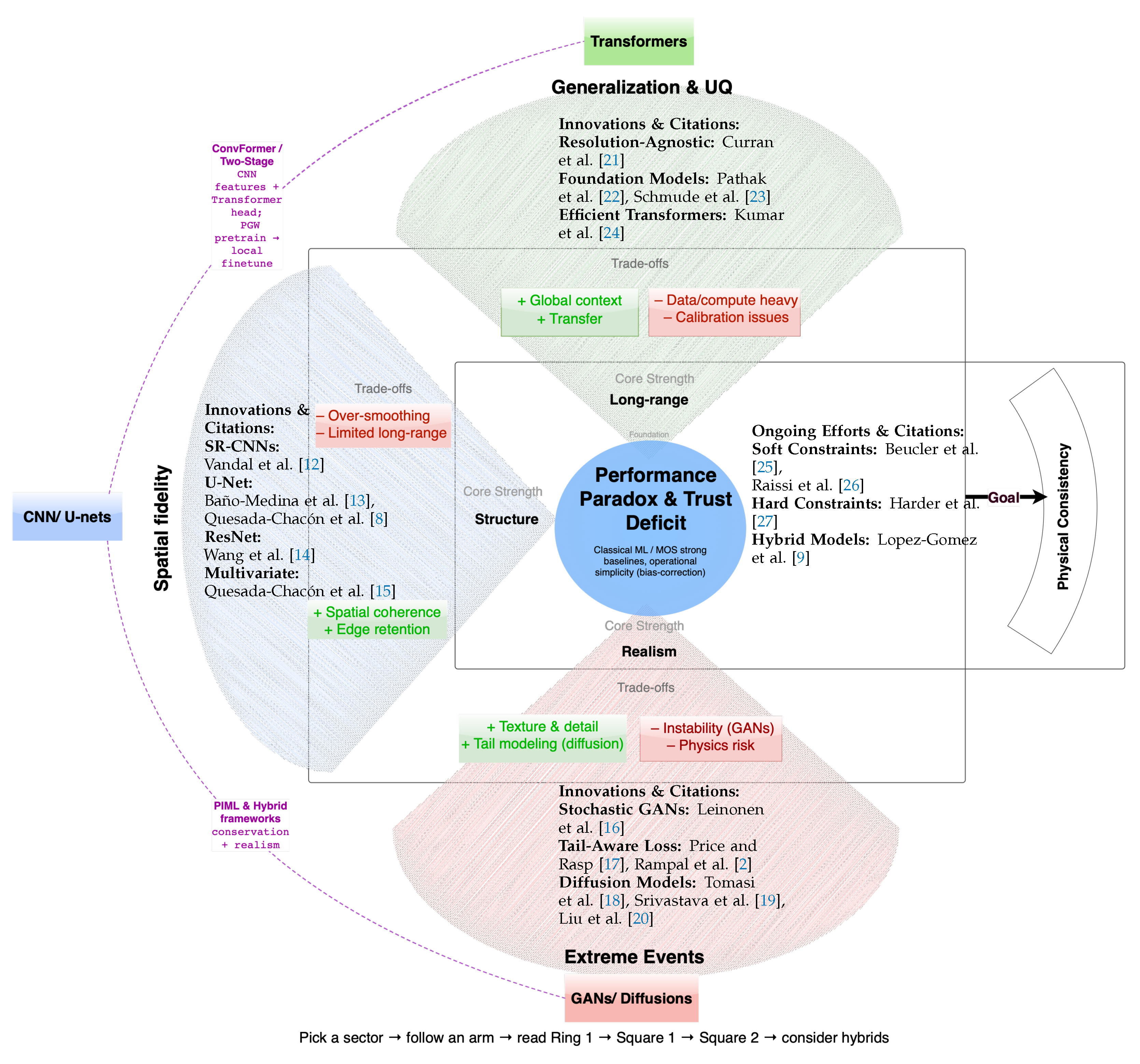
Figure 2.
A comparative overview of model families for climate downscaling tasks.
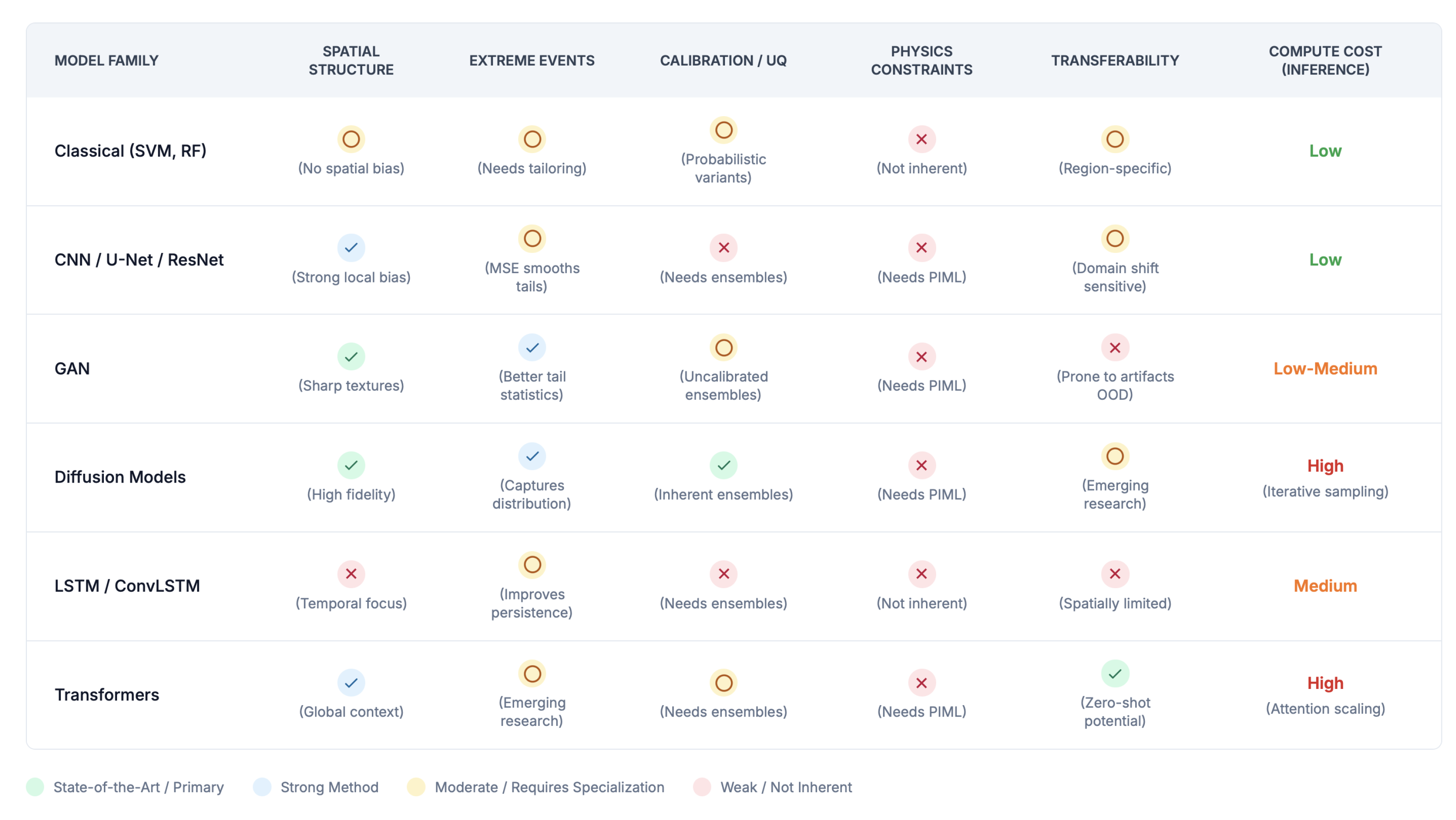
Figure 3.
A conceptual timeline illustrating the parallel evolution of ML models, scientific problem formulations, and the challenge of trust in climate downscaling from 2010–2025. As model power and realism have increased (right-hand axis), the inherent explainability of the models has decreased (left-hand axis), creating a “trust deficit.” This has spurred the development of new scientific questions and a counter-movement focused on rebuilding trust through XAI and PIML.
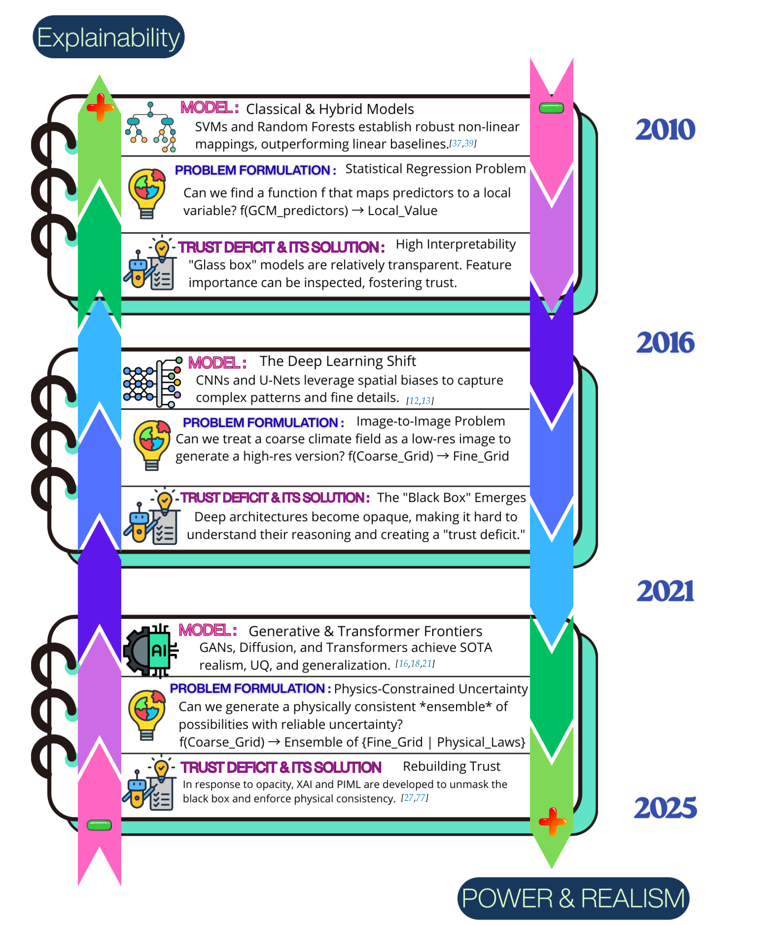
Figure 5.
Mapping robust validation techniques to the challenges they address, particularly for non-stationary climate data.
Figure 5.
Mapping robust validation techniques to the challenges they address, particularly for non-stationary climate data.
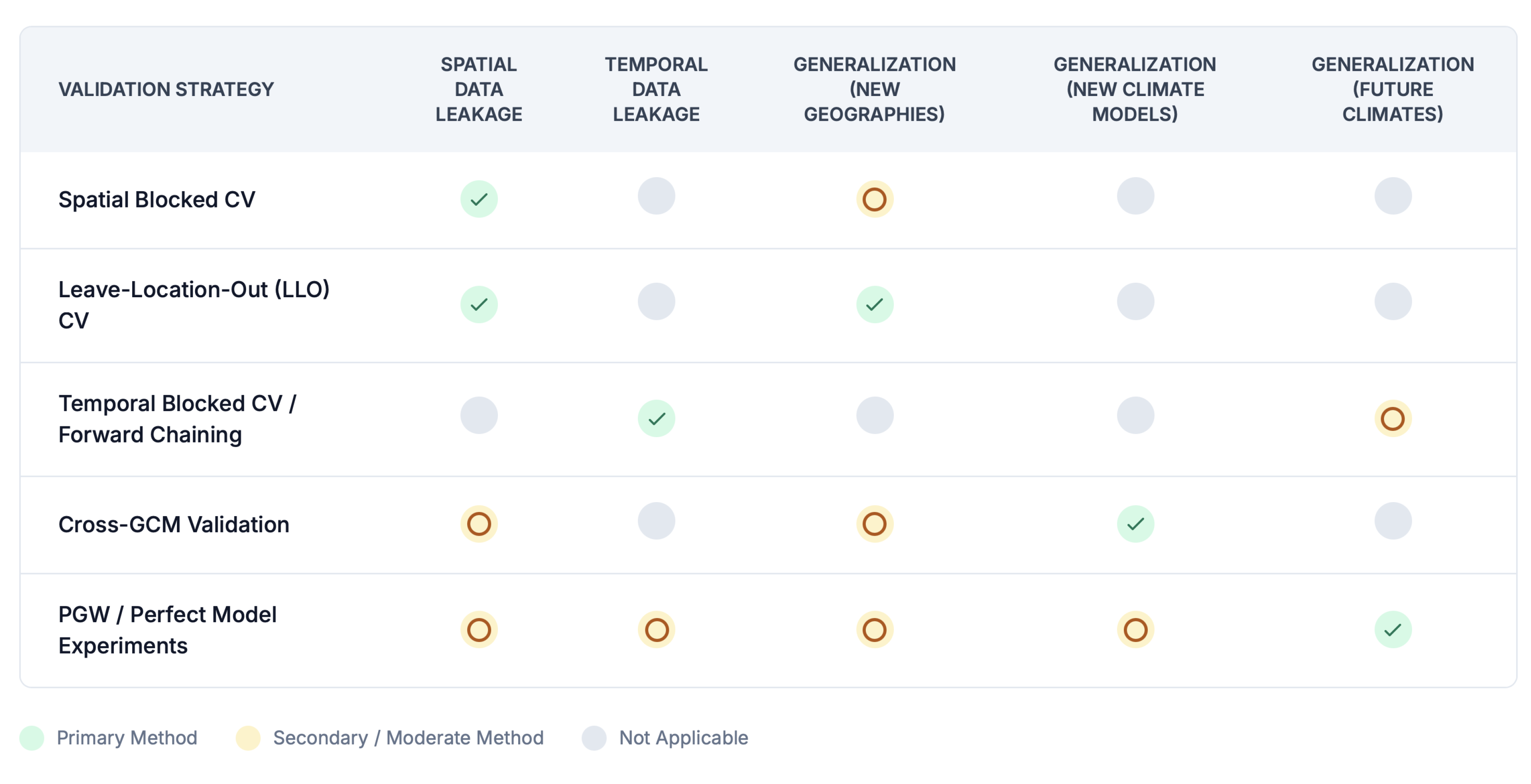

Table 1.
A Multi-faceted Evaluation Toolkit for ML-Based Downscalinga
| Category | Metric | Description & Use Case | When to Use | Key Refs |
|---|---|---|---|---|
| Pixel-wise Accuracy | RMSE / MAE | Root Mean Squared Error / Mean Absolute Error. Standard metrics for average error, but can be misleading for skewed distributions (e.g., precipitation) and penalize realistic high-frequency variations. | Standard baseline, but use with caution; supplement with other metrics. | [11] |
| Spatial Structure | Structural Similarity (SSIM) | Measures perceptual similarity between images based on luminance, contrast, and structure. Better than RMSE for assessing preservation of spatial patterns. | To evaluate preservation of spatial patterns and textures. | [55] |
| Power Spectral Density (PSD) | Compares the variance at different spatial frequencies. Crucial for diagnosing overly smooth outputs (loss of high-frequency power) or GAN-induced artifacts (spurious power). | To diagnose smoothing or unrealistic high-frequency noise. | [98,100] | |
| Variogram Analysis | Geostatistical tool that quantifies spatial correlation as a function of distance. Comparing nugget, sill, and range diagnoses noise, variance suppression, and incorrect spatial correlation length. | To quantitatively assess spatial dependency structure and diagnose over-smoothing. | [101] | |
| Method for Object-based Diagnostic Evaluation (MODE) | Identifies and compares attributes (e.g., area, location, orientation, intensity) of distinct objects (e.g., storms). Provides diagnostic information on specific spatial biases beyond grid-point errors. | For detailed diagnostic evaluation of precipitation fields, avoiding the "double penalty" issue. | [102,103] | |
| Temporal Coherence | Temporal Autocorrelation | Measures the correlation of a time series with itself at a given lag (e.g., lag-1 for daily data). Assesses the model’s ability to reproduce temporal persistence or "memory". | To diagnose unrealistic temporal "flickering" or lack of persistence in time series. | [104,105] |
| Wet/Dry Spell Characteristics | Quantifies the statistics of consecutive days above/below a threshold (e.g., 1 mm/day for precipitation). Key metrics include mean/max spell duration, frequency, and cumulative intensity. | Essential for impact studies related to droughts and floods; evaluates temporal clustering of events. | [106,107] | |
| Extreme Events | Fraction Skill Score (FSS) | A neighborhood-based verification metric that assesses the skill of forecasting events exceeding a certain threshold across different spatial scales. Mitigates the "double penalty" issue. | Essential for verifying precipitation fields at specific thresholds. | [96,100] |
| Quantile-based scores (e.g., 99th percentile error) | Directly evaluates the accuracy of specific quantiles (e.g., p95, p99), focusing on performance in the tails of the distribution. | To specifically quantify performance on rare, high-impact events. | [40] | |
| Return Level / Period Consistency | Compares the magnitude of extreme events for given return periods (e.g., the 1-in-100-year event) between the downscaled output and observations, often using Extreme Value Theory. | For climate impact studies where long-term risk from extremes is key. | [108] | |
| Distributional Similarity | Wasserstein Distance (Earth Mover’s Distance) | Measures the "work" required to transform one probability distribution into another. A robust measure of similarity between the full distributions of the downscaled and reference data. | For a rigorous comparison of the entire statistical distribution. | [20,109] |
| CRPS (Continuous Ranked Probability Score) | For probabilistic forecasts, measures the integrated squared difference between the predicted cumulative distribution function (CDF) and the observed value. A proper scoring rule that generalizes MAE. | Gold standard for evaluating probabilistic/ensemble forecast skill. | [97,100] | |
| Perkins Skill Score (PSS) | Measures the common overlapping area between two probability density functions (PDFs). An intuitive, distribution-agnostic metric of overall distributional similarity. | To provide a robust, integrated score of distributional overlap, common in climate model evaluation. | [110] | |
| Uncertainty Quantification (UQ) | Reliability Diagram | Plots observed frequencies against forecast probabilities for binned events to assess calibration. A perfectly calibrated model lies on the diagonal. | To assess if forecast probabilities are statistically reliable. | [100] |
| PIT Histogram | Probability Integral Transform. For a calibrated ensemble, the PIT values of the observations should be uniformly distributed. Deviations indicate biases or incorrect spread. | To diagnose issues with ensemble spread and bias. | [100] | |
| Physical Consistency | Conservation Error | Directly measures the violation of a conservation law (e.g., mass, energy) by comparing the aggregated high-resolution output to the coarse-resolution input value. | When conservation of a quantity is a critical physical constraint. | [25] |
| Multivariate Correlations | Assesses whether the physical relationships and correlations between different downscaled variables (e.g., temperature and humidity) are preserved realistically. | Essential for multi-variable downscaling to ensure physical coherence. | [9] | |
| Clausius-Clapeyron Scaling | Verifies if the intensity of extreme precipitation scales with temperature at the physically expected rate ( 7%/°C). Tests if the model has learned a fundamental thermodynamic relationship. | Critical for assessing the credibility of future projections of extremes under warming. | [111] |
aRecommended Minimum Evaluation Suite: For a robust evaluation, we recommend a core set of metrics. For spatial structure, report Variogram parameters (sill, range) and key MODE diagnostics (e.g., centroid error, area bias). For temporal coherence, report lag-1 autocorrelation and mean/max dry spell duration. For extremes, report FSS at relevant thresholds and the error at a high quantile (e.g., 99th). For distributional skill, report CRPS (if applicable) and Perkins Skill Score. For physical consistency, report Conservation Error and C-C Scaling rate.
Table 2.
Comparative Analysis of Dominant Machine Learning Architectures for Climate Downscaling. Note: Typical resolutions and UQ descriptions are illustrative; see key references for details.
Table 2.
Comparative Analysis of Dominant Machine Learning Architectures for Climate Downscaling. Note: Typical resolutions and UQ descriptions are illustrative; see key references for details.
| Architecture | Key Mechanisms/ Characteristics | Strengths in Downscaling | Limitations/ Weaknesses | UQ Capabilities / Robustness to Non-Stat. & Extremes | Typical Climate Variables | Typical Input Res. | Typical Output Res. | Key Refs |
|---|---|---|---|---|---|---|---|---|
| SVM (Support Vector Machines) | Kernel-based supervised learning; finds optimal hyperplane in transformed feature space; can use nonlinear kernels for complex relationships. | Performs well with limited data; robust to high-dimensional predictor spaces; strong baseline for PP downscaling. | Choice of kernel and hyperparameters critical; may underperform on highly non-stationary or extreme events; less scalable to massive training datasets. | UQ typically via bootstrapping or ensembles; deterministic by default; robustness to non-stationarity depends on training sample diversity. | Precip, Temp | GCM scale (e.g., 50–250 km) | Station/grid scale | [36,39] |
| Random Forests (RF, AP-RF, Prec-DWARF) | Ensemble of decision trees trained on bootstrap samples; output is mean/majority vote; AP-RF extends with predictive distribution outputs. | Handles nonlinear predictor–predictand relationships; naturally ranks predictor importance; AP-RF produces stochastic samples. | May smooth fine-scale details; bias in extremes without specialized treatment; interpretability less direct than single trees. | Yes for AP-RF (predictive distribution via gamma parameters); deterministic for standard RF; moderate robustness to non-stationarity if trained on diverse climates. | Precip | 0.25°–1° | 0.125° / site-level | [37,38] |
| CNN (SRCNN, U-Net, ResNet) | Convolutional layers, pooling, shared weights. U-Net: encoder–decoder w/ skip connections. ResNet: residual blocks. | Spatial feature extraction, pattern recognition; U-Nets preserve fine details; ResNets enable deeper learning. | Overfitting; extrapolation issues; can be overly smooth under MSE loss; plain CNNs struggle with depth. | UQ via ensembles; robustness to non-stationarity often limited without targeted strategies (e.g. PGW training). Standard CNNs may smooth extremes unless using specialized losses or architectures. | Temp, Precip, Wind, Solar Rad. | 25–250 km | 1–25 km | [10,12,44,46,49,122] |
| GAN (CGAN, MSG-GAN, evtGAN, Sup3rCC) | Generator and Discriminator trained adversarially. Conditional GANs (CGANs) use input conditions. Sup3rCC uses GANs to learn and inject spatio-temporal features from historical high-res data into coarse GCM outputs for renewable energy resource variables. | Perceptually realistic outputs, sharp details, better extreme event statistics, spatial variability. Sup3rCC provides high-resolution (4km hourly) realistic data for wind, solar, temp, humidity, pressure, tailored for energy system analysis and computationally efficient compared to dynamical downscaling. | Training instability (mode collapse), difficult evaluation, potential artifacts, may not capture the full statistical distribution. Sup3rCC does not represent specific historical weather events, but historical/future climate conditions, and does not reduce GCM uncertainty. | UQ via ensembles, but it can be challenging to calibrate. Potential for better extreme event generation. Robustness to Non-Stationarity is an active research area; can learn spurious correlations if not carefully designed/trained. Sup3rCC aims for physically realistic outputs by learning from historical data. | Temp, Precip, Wind, Solar Rad. Sup3rCC specialized for renewable energy variables (wind, solar, temp, humidity, pressure). | GCM scale (e.g., 25–100 km) | 1–12 km. Sup3rCC: 4km hourly. | [16,58,59,60,98,123,124,125] |
| LSTM / ConvLSTM | Recurrent memory cells (LSTM); ConvLSTM embeds convolutions into gates. | Captures long-range temporal dependencies; suitable for sequence modeling; CNN–LSTM hybrids. | High complexity; ConvLSTM outperforms pure LSTM on spatial data; very long-range spatial dependencies can be limited. | UQ via ensembles or Bayesian RNNs; can model temporal non-stationarity if reflected in training data but may struggle with unseen future shifts and rare extremes without augmentation. | Precip, Runoff, other time-evolving vars. | Gridded time series | Gridded time series | [43,68,69,115] |
| Transformer (ViT, PrecipFormer, etc.) | Self-attention for global context; captures long-range spatio-temporal interactions. | Excellent at modeling long-range dependencies; strong transfer potential, especially in hybrid architectures. | Quadratic attention cost (being mitigated by sparse/linearized variants); relatively new in downscaling; large data requirements. | UQ via attention-weighted ensembles; promising for non-stationarity when pre-trained on diverse climates; attention can focus on localized antecedent signatures of extremes, aiding detection though not guaranteeing tail magnitude accuracy. | Temp, Precip, Wind, multiple vars. | Various (e.g., 50 km, 250 km) | Various (e.g., 0.9 km, 7 km, 25 km) | [21,23,24,65,66,71] |
| Diffusion Model (LDM, STVD) | Iterative denoising process; LDMs operate in latent space. | High-quality, diverse samples; stable training; explicit probabilistic outputs; good spatial detail. | Computationally intensive (though LDMs mitigate cost); relatively nascent for downscaling; slow sampling. | Excellent UQ via learned distributions and ensemble generation; promising for capturing tail behavior and fine-grained spatial detail of extremes ; robustness to non-stationarity is an active research area, but shows potential when trained on diverse climate data. | Temp, Precip, Wind | 100–250 km | 2–10 km | [18,19,20,31,63] |
| Multi-task Foundation Models (e.g., Prithvi-WxC, FourCastNet, ORBIT-2) | Large pre-trained (often Transformer-based) models fine-tuned for downscaling. | Zero/few-shot potential; multi-variable support; leverage extensive pre-training. | Very high pre-training cost; uncertain generalization to new locales/tasks without adaptation; bias propagation risks. | UQ via large-ensemble sampling; pre-training on diverse climates can enhance robustness to non-stationarity and extremes, but careful domain adaptation is essential. | Multiple vars | Coarse GCM / Reanalysis | Fine (task-dependent) | [22,74] |
Disclaimer/Publisher’s Note: The statements, opinions and data contained in all publications are solely those of the individual author(s) and contributor(s) and not of MDPI and/or the editor(s). MDPI and/or the editor(s) disclaim responsibility for any injury to people or property resulting from any ideas, methods, instructions or products referred to in the content. |
© 2025 by the authors. Licensee MDPI, Basel, Switzerland. This article is an open access article distributed under the terms and conditions of the Creative Commons Attribution (CC BY) license (http://creativecommons.org/licenses/by/4.0/).
Copyright: This open access article is published under a Creative Commons CC BY 4.0 license, which permit the free download, distribution, and reuse, provided that the author and preprint are cited in any reuse.


