Submitted:
17 November 2025
Posted:
18 November 2025
You are already at the latest version
Abstract
This paper proposes an intelligent and explainable ensemble system for predicting as-partate aminotransferase (AST) levels based on routine biochemical and demographic data from the NHANES dataset. The framework integrates robust preprocessing, adaptive feature encoding, and multi-level ensemble learning within a nested cross-validation (5×3) structure to ensure reproducibility and prevent data leakage. Several regression mod-els—including Random Forest, XGBoost, CatBoost, and stacking ensembles—were sys-tematically compared using R², RMSE, MAE, and MAPE metrics. The results show that the Stacking v2 architecture, combining CatBoost, LightGBM, and Ridge meta-regression, achieves the highest predictive accuracy and stability. Explainable AI analysis using SHAP revealed key biochemical and lifestyle factors influencing AST variability. The pro-posed system provides a modular, interpretable, and reproducible foundation for deci-sion-support applications in intelligent healthcare analytics, aligning with the goals of applied system innovation.
Keywords:
ensemble learning
; stacking
; AST prediction
; explainable AI
; SHAP
; regression algorithms
; medical machine learning
; NHANES
; biomedical data
1. Introduction
The rapid development of artificial intelligence and data analytics has transformed traditional biomedical analysis into an integrated system of intelligent decision-support tools [1,2,3]. In predictive medicine, routine biochemical markers such as aspartate ami-notransferase (AST) serve as critical indicators of metabolic imbalance and tissue dys-function [4,5]. However, extracting actionable insights from heterogeneous health data remains a systemic challenge due to data variability, nonlinear relationships, and the need for interpretability [6]. Within the paradigm of applied system innovation, machine learning can be viewed not only as an algorithmic tool but also as a core component of in-telligent information systems that process biomedical signals, learn from population data, and support evidence-based decisions [7,8]. Ensemble learning approaches such as Ran-dom Forest, XGBoost, and CatBoost have proven effective for handling complex depend-encies and improving robustness across diverse datasets [9,10]. Nevertheless, the lack of transparency in predictive models limits their deployment in real-world healthcare sys-tems, motivating the integration of explainable artificial intelligence (XAI) techniques and reproducible modeling frameworks [11,12].
This paper proposes a modular, interpretable, and reproducible ensemble framework for predicting AST levels from the publicly available NHANES dataset (1988–2018) [13]. The system incorporates robust preprocessing, adaptive encoding, and nested cross-validation (5×3) to ensure methodological reliability and prevent information leak-age [14]. The framework compares several regression algorithms—Linear Regression, Random Forest, XGBoost, CatBoost, and stacking architectures—using multiple perfor-mance metrics (R², RMSE, MAE, and MAPE). The results demonstrate that stacking en-sembles with CatBoost and Ridge meta-regression outperform traditional models while maintaining interpretability through SHAP-based explanations [15]. From a sys-tem-engineering perspective, the proposed framework represents a scalable and repro-ducible foundation for intelligent healthcare analytics and decision-support systems. By emphasizing explainability, robustness, and modular integration, this study contributes to the ongoing evolution of applied intelligent systems in biomedical data science.
The remainder of this paper is organized as follows. Section 2 reviews related studies on the application of machine learning methods for biochemical and clinical data analy-sis. Section 3 describes the dataset, data preprocessing workflow, and methodological framework of the proposed system, including the ensemble architectures and cross-validation strategy. Section 4 presents the experimental setup and comparative re-sults of different regression models. Section 5 discusses the interpretability analysis, key findings, and system-level implications for intelligent healthcare applications. Finally, Section 6 concludes the paper and outlines future research directions aimed at extending the framework into real-time decision-support environments.
2. Related Works
In recent years, more research has focused on predicting liver enzyme levels, including aspartate aminotransferase (AST), using machine learning methods. Hu et al. [16] found a link between a high ALT/AST ratio and the risk of liver fibrosis based on NHANES data, but they did not concentrate on predicting individual AST levels. Zhu et al. [17] proposed a Random Forest model to estimate the risk of elevated transaminases in patients with rheumatoid arthritis, achieving high accuracy but limited to a narrow clinical cohort. A broader approach was proposed by Yang et al. [18], who developed machine learning models for diagnosing MASLD using routine data; AST levels were considered only indirectly. Interpretable models are also gaining momentum. Wang et al. [19] utilized SHAP to explain predictions from NAFLD ML models, demonstrating the potential of such solutions for medical interpretation. In turn, Ali et al. [20] confirmed the possibility of diagnosing cardiovascular diseases using routine blood tests and ensemble models, but liver biomarkers were not the subject of analysis. In addition, Yang et al. [21] presented a systematic review of the application of machine learning (ML) in predicting outcomes after liver transplantation, demonstrating advantages over traditional scoring systems; however, they did not address the aspect of routine screening. Khaled et al. [22] proposed a deep learning system for the early detection of liver diseases, which requires further clinical validation. McGettigan [23] investigated the performance of various machine learning (ML) models on an extensive array of medical data, confirming the potential of the algorithms for liver diagnostics but without specifying the specific architectures. Farhadi et al. [24] studied how to predict complications after recovery from hepatitis B. This focus limits how widely their model can be applied. Table 1 shows that all these studies highlight the need for specialized and clear models that focus on individual risk for elevated AST, using available clinical, demographic, and biochemical data.
As shown in Table 1, the majority of current studies confirm the high efficiency of machine learning methods for analyzing and predicting diseases based on routine medical data. However, only a few studies directly focus on predicting AST levels as a separate biomarker. Additionally, some studies use models that are hard to interpret, which limits their use in clinical practice. The identified scientific gaps, including poor generalizability, a lack of multivariate analysis, and weak integration of behavioral factors, highlight the need to create a complete model for predicting the risk of AST elevation based on available and standardized indicators. Despite the active development of machine learning in biomedicine, most existing studies focus on predicting diseases in tissues with high metabolic activity and do not consider aspartate aminotransferase (AST) as a significant marker of cardiovascular risk.
In addition to existing literature on liver biomarkers and clinical machine learning, recent advancements in machine learning theory and biomedical applications provide valuable methodological insights relevant to our study. For instance, reinforcement learning techniques applied in robotic gait design [25] and inverse reinforcement learning offer frameworks for adaptive optimization. Multi-modal and self-paced learning strategies, as explored in Alzheimer’s diagnostics [26], demonstrate the benefits of progressive and locality-preserving learning, which could be translated to biomedical feature structuring. Boundary refinement techniques [27] and subsampling methods for partial least squares regression [28] further highlight the importance of robust feature interaction modeling and efficient dimensionality reduction. These methodological perspectives align with our use of SHAP, mediator analysis, and ensemble meta-learning to ensure model interpretability and generalizability in clinical prediction tasks.
This study presents an understudied yet promising approach for predicting cardiovascular diseases using AST and other routine indicators. Distinctive features of this work include:
- Direct regression prediction of AST level, considered as an independent predictor of cardiovascular risk and not as a marker of hepatological disorders;
- Integration of routine biochemical, anthropometric, and behavioral parameters, including inflammation, body weight, and lifestyle indicators, enhances the clinical relevance of the model;
- Use of a stacking ensemble (Stacking v2), which combines the capabilities of modern algorithms and an interpretable meta-model to improve accuracy and stability;
- The use of SHAP and mutual information to analyze the significance of features ensures the interpretability of the model and its applicability in the clinical environment;
- Validation on a large and representative NHANES dataset (1988–2018) covering a wide range of health data from the US population.
Unlike previous studies limited to narrow clinical cohorts or liver disease diagnostic tasks, our study demonstrates how routine parameters, including AST, can be effectively used to assess cardiovascular disease risk in the general population. The proposed model may become a tool for early screening and personalized prevention in resource-limited settings.
3. Materials and Methods
The proposed system is designed as a modular and reproducible intelligent frame-work consisting of four components: (1) data acquisition from the NHANES repository, (2) preprocessing and feature engineering, (3) ensemble machine learning and optimization, and (4) interpretability and decision-support output. This architecture enables scalability and integration into intelligent healthcare systems, aligning with the concept of applied system innovation.
This study used data from the National Health and Nutrition Examination Survey (NHANES) for the period 1988–2018, including biochemical, demographic, and behavioral parameters of respondents. This source provides a representative dataset on the health status of the US population and is widely used for scientific purposes [13,14]. The study included routine biochemical markers, such as ferritin, glucose, γ-glutamyltransferase (γ-GT), and lactate dehydrogenase (LDH), as well as data on lifestyle, body weight, and physical activity level [15]. Comprehensive data preprocessing was carried out: removing outliers, eliminating gaps, standardizing numerical features, and coding categorical variables, which is a necessary step for building reliable machine learning models [29,30]. Based on the prepared data, different machine learning models were trained and compared to predict the risk of elevated aspartate aminotransferase (AST) [31].
3.1. Dataset Collection
To create a model for predicting aspartate aminotransferase (AST) levels, we used the national dataset from the National Health and Nutrition Examination Survey (NHANES) covering the years 1988 to 2018. This source offers extensive information on the health status of the US population, including biochemical analysis data, body measurements, and details on behavior and demographics. NHANES was selected for its representative nature, standard data collection methods, and high reliability. We focused on records from adult respondents (aged 18 and older) with available AST values and other key indicators. These included ferritin, γ-glutamyl transferase (γ-GT), lactate dehydrogenase (LDH), glucose, body mass index, physical activity, smoking, alcohol consumption habits, and inflammation indicators. Incomplete observations and abnormal values were excluded, and data cleaning and standardization procedures were performed. All features are brought to a single format, categorical variables are coded, and numerical variables are normalized. As a result, a structured sample is formed, suitable for the application of machine learning algorithms. It covers various aspects of the physiological state and lifestyle of respondents, providing a basis for constructing an interpretable prognostic model—the original data presented at https://drive.google.com/drive/folders/1cgyQXj3Kl7FdDoyPlmEkCKyDXNDIv4JB?usp=drive_link (accessed on 06 June 2025).
The threshold “s ≤ 200” refers to AST values and was applied to exclude extreme outliers in the dataset. Both clinical and statistical rationale support this choice. Clinically, AST values above 200 U/L are often indicative of acute hepatocellular injury (e.g., severe hepatitis or liver necrosis), which falls outside the subclinical or routine screening contexts that our model targets. Statistically, preliminary distributional analysis of AST in NHANES revealed a heavy right-skew, with the 99th percentile around 80 U/L and values >200 U/L observed in <0.5% of the population. Furthermore, an IQR-based method yielded an upper bound of approximately 180–210 U/L; we conservatively rounded this to 200 U/L to provide a simple, reproducible threshold for filtering rare, high-leverage outliers. This filtering step enhances model calibration and preserves its applicability to routine cases, particularly in early screening scenarios.
To ensure data completeness and reliable modeling, rows with missing values were removed using the listwise deletion method. Specifically, only those observations were retained where all values were present for the full set of features used in the current stage of analysis, including the target variable (LBXSASSI — AST level). The considered variables included: age (RIDAGEYR), gender (RIAGENDR), body weight (BMXWT), height (BMXHT), ferritin (LBXFER), homocysteine (LBXHCY), total cholesterol (LBXTC), LDL-C (LBDLDL), glucose (LBXGLU), hemoglobin (LBXHGB), creatinine (LBXSCR), hs-CRP (LBXCRP), alkaline phosphatase (LBXSAPSI), gamma-glutamyl transferase (LBXSGTSI), lactate dehydrogenase (LBXSLDSI), uric acid (LBXSUA), leukocytes (LBXWBCSI), alcohol intake (ALQ130), physical activity (PAD615), and the target AST marker (LBXSASSI). Any row with at least one missing value in this set was excluded from further analysis. This approach ensured that only complete cases were included in the modeling process, thus improving statistical validity and interpretability of the results.
Initially, missingness was assessed across all predictor variables, including key clinical and biochemical features such as age, BMI, glucose, creatinine, albumin, ALT, AST, GGT, LDH, and gender (RIAGENDR). However, rather than applying listwise deletion, which would have led to the exclusion of approximately 35% of the dataset, we implemented a model-specific imputation strategy. Only records missing the target variable (AST) or containing implausible AST values (>200 U/L) were permanently removed. This approach allowed us to retain a more comprehensive feature set and significantly increase the effective sample size while maintaining data integrity.
3.2. Rationale for a Method Selection
Building an effective predictive model required the use of a complex algorithm that included several interrelated stages of data preprocessing, feature selection, and model ensemble training. Each method in this process was selected based on its robustness, efficiency, and applicability to medical data with heterogeneous features.
- Removing emissions. In the first step, we excluded observations with suspiciously high values (s ≤ 200) from the dataset. This helps reduce the influence of anomalies and noise on model training. It's especially important when dealing with biomarkers, as technical or clinical errors can lead to outliers.
- Removing gaps. Removing rows with missing values in the target variable (AST) and critical predictors ensures the correctness of the training process. This step is necessary to maintain the quality of predictions and prevent distortions.
- Transformation of categorical variables. One-hot encoding of categorical features (e.g., demographic and questionnaire data) is applied, which allows them to be efficiently included in machine learning models without violating assumptions about the numerical nature of the input data.
- Scaling of Numerical Features. Numerical features are normalized (z-transformed) to equalize scales and prevent features with high variance from dominating the analysis. This is especially important for linear and gradient-boosted models that are sensitive to scale.
- Split into training and validation samples. The standard split of the sample (train/test split) is used to assess the quality of the model objectively. This allows you to control overfitting and tune hyperparameters.
- Base models (Base regressors). The following algorithms were selected to build a forecast of the AST level:
- Linear Regression — a basic benchmark for estimating linear relationships.
- Random Forest — a stochastic model that is robust to outliers and works well with small samples.
- XGBoost — a powerful gradient boosting that provides high accuracy and control over overfitting.
- CatBoost — an optimized boosting algorithm that works efficiently with categorical features without the need for manual coding.
- LightGBM — a fast and scalable boosting algorithm, especially effective on large and sparse data.
- Extra Trees — an improved version of Random Forest that uses additional stochasticity to improve generalization.
- 7.
- Stacking. As shown in Figure 1, Stacking v1 is a simple two-level ensemble scheme in which base models (Linear Regression, Random Forest, and XGBoost) are independently trained on the original features (1):
Stacking v2 is an advanced two-level ensemble model that utilizes modern and powerful algorithms as base models, including CatBoost, LightGBM, and ExtraTrees, which provide high accuracy through boosting and stochastic approaches (2):
where - vector of initial features for the i-th object (observation) from the training sample, — vector of Ridge regression coefficients, α>0— L2 regularization coefficient.
At the second level, a Ridge regression meta-model is used, which is robust to multicollinearity and prone to regularization, thereby reducing the risk of overfitting and accounting for the possible correlation between the predictions of the base models. The final prediction is formed based on the outputs of these three ensembles, aggregated using Ridge regression. Among the advantages of Stacking v2 are high accuracy, resistance to overfitting, and good adaptation to nonlinear dependencies (Figure 2). The main disadvantages are the increased complexity of hyperparameter tuning and increased computational costs compared to simpler schemes such as Stacking_v1.
Figure 3 presents the most advanced and outlier-robust ensemble architecture, which includes powerful base models — CatBoost, LightGBM, XGBoost, Random Forest, and a specialized regressor for predicting high AST values (HighAST Regressor) (3):
where
- vector of initial features for the i-th object (observation) from the training sample.
In the second level of Stacking_v3, the meta-model is LGBMRegressor with the objective="huber" parameter. This means that optimization occurs using the robust Huber loss, which is resistant to outliers and more flexible than MSE. All boosted models utilize Huber loss (4), which ensures robustness to outliers and asymmetric errors.
where — true meaning, — model prediction, δ=2.0 (for CatBoost, or by default in LGBM), — indicator function.
LightGBM is used as a meta-model with the same loss function and a "passthrough" mode, in which the meta-algorithm receives not only the predictions of the base models but also the original features, which allows it to effectively restore complex dependencies and compensate for the weaknesses of individual models. The final forecast is formed based on cumulative information, making this scheme the most robust against various types of errors. Its advantages include high accuracy, robustness to outliers, the ability to use rare patterns through the HighAST model, and a detailed feature representation. However, the model requires a lot of computing power, careful tuning of hyperparameters, and effective management of overfitting. Despite its complexity, the model did not show significant benefits on validation data for several important metrics, such as R², RMSE, and MAE. This indicates the need for further analysis and possibly adjustments to the model's structure.
Overall, the Stacking_v2 architecture was optimal in terms of the combination of accuracy, stability, and interpretability criteria. It is recommended to use this option for predicting the AST level using the presented markers and features.
3.3. Stages of Model Implementation
Proper feature selection plays a key role in building accurate and interpretable machine learning models, especially in the clinical context, where each variable can reflect critical biomedical processes. Based on biochemical, anthropometric, and behavioral characteristics, as well as the use of explainable AI approaches, an assessment is carried out to evaluate their contribution to the predicted variable. This analysis not only improves the quality of prediction but also identifies pathophysiological relationships that are crucial for interpreting results and informing clinical practice.
I. Notations and variables used
- n — number of observations (patients);
- d — number of initial features;
- feature matrix;
- feature vector for the i-th patient;
- target variable vector (ACT level, LBXSASSI).
Trait variables:
- ▪
- — age;
- ▪
- — gender;
- ▪
- — weight;
- ▪
- — height;
- ▪
- — ferritin;
- ▪
- — homocysteine;
- ▪
- — total cholesterol;
- ▪
- — LDL-C;
- ▪
- — glucose;
- ▪
- — hemoglobin;
- ▪
- — creatinine;
- ▪
- — hs-CRP;
- ▪
- — alkaline phosphatase (ALP);
- ▪
- — gamma-GT;
- ▪
- — LDH;
- ▪
- — urea;
- ▪
- — uric acid;
- ▪
- — leukocytes;
- ▪
- average number of alcoholic drinks per day;
- ▪
- — physical activity.
Figure 4 shows the complete architecture of the algorithm for constructing a predictive model for the aspartate aminotransferase (AST) level, including the stages of data preprocessing, feature selection, training of base models, and formation of the Stacking_v2 ensemble. The algorithm begins by removing outliers and missing values, then encodes categorical variables and scales numerical features. After splitting into training and validation samples, several regressors are trained in parallel (including XGBoost, CatBoost, LightGBM, ExtraTrees, etc.), and the final model is formed using meta-regression based on these models.
Records with non-zero target values of AST (LBXSASSI) and biologically plausible levels (AST ≤ 200 U/L) were selected, thereby excluding extreme outliers. Subsequently, a model-specific preprocessing pipeline was implemented within a nested cross-validation (nested CV) framework using a 5×3 scheme.
- For CatBoost: the gender feature (RIAGENDR) was converted to a categorical type (object), with missing values explicitly marked as "__MISSING__". All other features were retained in their numeric form. No one-hot encoding (OHE) or feature scaling was applied, as CatBoost natively handles both categorical variables and missing values.
- For Random Forest, XGBoost, and Stacking models: numerical features with missing values were imputed using SimpleImputer(strategy="median") to support tree-based models and meta-learners. The gender feature (RIAGENDR) was encoded using OneHotEncoder(handle_unknown="ignore"). Feature scaling was selectively applied only where necessary (e.g., for linear models or the meta-level in stacking).
All preprocessing steps, hyperparameter tuning, and model evaluation were performed strictly within the folds of the nested CV to prevent data leakage. The outer loop employed 5-fold KFold cross-validation with shuffle=True and random_state=42, generating five independent test subsets . For each outer fold t, a 3-fold inner loop (KFold, shuffle=True, random_state=43) was used for hyperparameter tuning via GridSearchCV, optimizing for the R² metric. After selecting the optimal hyperparameters , preprocessing transformers were re-fitted on the full training set , and the model was trained and evaluated on the corresponding test set only. Performance metrics — including R², RMSE, MAE, MAPE, and Explained Variance — were aggregated across the five outer folds, with 95% confidence intervals calculated to provide a robust estimation of generalization performance. For final demonstration, an ensemble model (Stacking_v2) was employed: the first layer consisted of CatBoost, LightGBM, and ExtraTrees regressors; the second layer used a Ridge regressor (without passthrough) as the meta-model to aggregate base-level predictions. This architecture combines robustness to outliers, effective handling of categorical variables, and reproducible validation using the nested CV 5×3 scheme.
II. Steps of data preparation and processing
- Loading and merging data. The first stage involves loading three tables containing clinical, demographic, and questionnaire data, after which they are combined using a unique patient identifier (SEQN), allowing for the formation of a single data structure for subsequent analysis and model building (4).
- Remove outliers. Removes records where the target variable (5)
- Removing gaps. Only those records are left where there are no gaps for the selected features and target variable (6):
- Transformation of categorical variables. Gender indicator is encoded using the one-hot method (7):
- Scaling of numerical features. For each numerical feature ()), except for categorical ones, standardization is applied (8):
III. Mathematical description of model training
- Training base regressors. For each base algorithm we train a regression function (9):
- — Linear Regression
- — Random Forest
- — XGBoost
- — CatBoost
- — LightGBM
- — Extra Trees
- local regressor for high AST values (trains only on cases with y>50)
IV. Methods of selection and analysis of features
1. Correlation analysis
- Linear correlation (10):
- pearman/Kendall: uses nonparametric measures for robustness.
- Mutual Information (11):
- SHAP values (12):
Stacking v2. The final model is a second-level ensemble combining the predictions of the base models using ridge regression as a meta-algorithm. This approach enables the extraction of advantages from different models, thereby increasing the stability of predictions and reducing error due to aggregation. The use of stacking is especially justified in problems where there is no single universal predictor, and it is necessary to combine knowledge from different sources. Taken together, the described methodological approach enables the construction of an interpretable, robust, and accurate model for predicting the AST level based on available routine data, offering high potential for clinical application.
To address concerns regarding the cross-validation strategy, all models—including base regressors and stacking ensembles (Stacking_v1–v3)—were evaluated using a rigorous nested cross-validation protocol (5×3), ensuring unbiased performance estimation. Specifically, hyperparameter tuning was conducted exclusively within the inner loop (3-fold KFold, shuffle=True, random_state=43), while the outer loop (5-fold KFold, shuffle=True, random_state=42) was used to assess generalization ability on unseen data. The second-level stacking meta-models were also trained and optimized within this nested structure. All preprocessing steps (e.g., imputation, encoding, scaling) were embedded within the modeling pipelines and retrained independently within each fold to avoid data leakage, thereby guaranteeing methodological robustness and reproducibility (Table 2).
The table summarizes the structure and key hyperparameters of all tested models, encompassing both interpretable baselines and advanced ensemble techniques. Linear Regression served as a reference point, while tree-based models such as Random Forest and XGBoost provided nonlinear benchmarks. CatBoost was configured with adaptive loss selection (Huber or RMSE) depending on internal cross-validation performance. The stacking ensembles differed in base model composition, meta-regressor type, and passthrough mode. Notably, Stacking_v2 employed Ridge regression for robust aggregation of strong base learners, whereas Stacking_v3 incorporated a specialized HighASTRegressor trained on elevated AST values (y > 50) to enhance performance in high-risk subpopulations. All configurations were tuned within a nested CV framework, ensuring fair comparisons and reliable generalization estimates.
4. Results
This study was conducted using the publicly available, harmonized NHANES 1988–2018 (National Health and Nutrition Examination Survey) dataset, which combines national data on the health and nutrition status of the US population over 30 years [9]. Thanks to complex preprocessing, this resource ensures high comparability of variables and minimizes the impact of missing and erroneous values, which is critical for building valid machine learning models. The selection of features for analysis was carried out strictly by the goal of the study - to develop an accurate and accessible model for predicting aspartate aminotransferase (AST) levels based exclusively on low-cost and routine biochemical markers that are available as part of standard medical examinations, without the use of specialized and expensive cardiology tests.
The final dataset for building the prognostic model included 21 accessible and clinically relevant variables. Demographic characteristics, such as age and gender, served as baseline covariates to account for individual variability. Anthropometric indicators (e.g., body weight and height) reflected metabolic load and general physiological condition. Key biochemical markers—ferritin, homocysteine, cholesterol, glucose, creatinine, hemoglobin, hs-CRP, urea, uric acid, and leukocytes—were selected to characterize metabolic, inflammatory, renal, hepatic, and hematologic functions. Inexpensive but informative liver enzymes, including γ-glutamyl transferase (γ-GT), lactate dehydrogenase (LDH), and alkaline phosphatase, were used as practical alternatives to specialized liver function tests. Behavioral factors such as alcohol consumption and physical activity were also included to capture lifestyle-related influences.
4.1. Assessment of Forecast Quality
This feature selection strategy enhances the model’s practical applicability, as it relies exclusively on routine clinical data that are widely available and cost-effective, making it suitable for large-scale population screening. Prior to modeling, all numerical features were standardized and categorical variables were one-hot encoded. The datasets were merged using unique participant identifiers, followed by the exclusion of missing or extreme values.
Table 3 presents summary statistics (N, Min, 25th percentile, Median, 75th percentile, Max, and IQR) for each variable. After filtering, the intermediate analytic sample comprised 131,030 patients. Of the initial 201,850 records, 70,820 were excluded due to missing values or biologically implausible entries, including 73 cases with AST values exceeding 200 U/L. The broad ranges and interquartile spreads observed confirm the high heterogeneity of the population and highlight the need for robust, multifactorial modeling in predicting AST levels. To further refine the dataset, records without the target variable and those with extreme AST values (>200 U/L) were excluded, resulting in a final analytical cohort of 63,524 observations. Among the initial dataset, approximately 70,820 records contained missing values; however, by applying median imputation within the training folds of the nested cross-validation framework, a substantial proportion of incomplete records was retained. Numerical features were imputed using fold-specific medians, while categorical variables were either one-hot encoded (for Random Forest and XGBoost) or handled natively (CatBoost). This preprocessing strategy significantly enhanced the size and representativeness of the final sample, improved statistical power, and ensured the robustness of modeling to data incompleteness—without compromising methodological rigor.
To build a predictive model, both basic algorithms and various ensemble schemes were tested. Both interpretable (linear regression) and more powerful ensembles — Random Forest, XGBoost, and CatBoost were used as single models. In addition, three versions of stacking models were implemented, differing in the composition of the basic models, meta-algorithm, and the use of additional strategies. All models were tuned to optimize the parameters that strike a balance between accuracy and stability. Table 4 presents brief characteristics of the models used and the key hyperparameters applied in the experiment.
As shown in Table 4, each model had its specific settings and architecture. Simple models, such as linear regression, were primarily used for basic comparison, while ensemble approaches, especially Stacking_v2, yielded the best results across several metrics. Of particular interest are complex configurations, such as Stacking_v3, and a specialized regressor for the subsample with high AST values, focused on handling outliers and complex cases. This multi-level approach allowed us to comprehensively evaluate the potential of various algorithms in predicting biomarkers on routine data. A set of validated metrics was used for a comprehensive assessment of the predictive abilities of the trained models.
A comprehensive assessment of the predictive ability was performed using the R², RMSE, MAE, MAPE, and Explained Variance metrics calculated on external test folds and then averaged (with 95% CI). The graphical comparison (Figure 5) shows the distribution of R² across external folds for all models (Linear Regression, Random Forest, XGBoost, CatBoost, and three stacking options), which ensures a correct comparison without inflating the results.
Figure 5 presents the comparison of model performance (R² metric) when trained on the full feature set versus a reduced feature set excluding GGT and LDH values. The results consistently demonstrate that the removal of GGT and LDH leads to a noticeable decline in predictive performance across all models, underscoring the relevance of these features in estimating AST levels. For instance, Linear Regression shows a drastic drop in R² from 0.256 to 0.080, highlighting its sensitivity to the exclusion of key biochemical features. Random Forest and XGBoost also exhibit substantial declines: from 0.442 to 0.199 and from 0.649 to 0.451, respectively. CatBoost, known for its ability to handle categorical features and missing data, maintains relatively stable performance (0.502 vs. 0.254), though still showing a significant drop. The most robust results are observed in the stacking ensembles. The Stacking_v2 model achieves the highest R² of 0.749 with the full feature set, decreasing to 0.658 without GGT/LDH. Even the simplified Stacking_v3 ensemble sees a reduction from 0.498 to 0.342. These findings confirm that including GGT and LDH contributes meaningfully to model accuracy and should be retained in predictive pipelines unless explicitly unavailable. Overall, this comparative analysis highlights the importance of GGT and LDH in modeling AST levels and supports their inclusion for enhanced predictive reliability in clinical datasets.
To evaluate the importance of specific biochemical features, we conducted an ablation analysis comparing model performance on the full feature set versus a reduced set excluding GGT and LDH markers. The evaluation was carried out using RMSE as the metric, with lower values indicating better predictive accuracy. All models were trained and validated using nested cross-validation to ensure reliable performance estimation and prevent data leakage (Figure 6).
As shown in Figure 6, the exclusion of GGT and LDH results in increased RMSE across all models, indicating a deterioration in prediction accuracy. For example, RMSE increased from 9.867 to 10.972 for Linear Regression and from 8.075 to 9.880 for CatBoost. The most accurate results on the full feature set were achieved by Stacking_v2 (RMSE = 5.731), which also showed degradation without GGT/LDH (RMSE = 6.888). These findings highlight the predictive contribution of GGT and LDH in estimating AST levels and support their inclusion in biomedical modeling pipelines.
To further assess the predictive stability of models with and without enzymatic biomarkers GGT and LDH, we compared the MAE across multiple algorithms, including linear, ensemble, and stacking-based approaches. MAE is a robust metric for evaluating prediction accuracy, as it captures average absolute deviations without being disproportionately influenced by large outliers. This metric provides insight into the typical error size across predictions, especially useful for medical regression problems (Figure 7).
As shown in Figure 7, models trained on the full feature set consistently achieved lower MAE values compared to their counterparts lacking GGT and LDH, reaffirming the importance of these enzymatic features in improving prediction accuracy. The lowest MAE was obtained by the Stacking_v2 model using the full feature set (2.948), while performance declined notably when these features were excluded (3.334). This trend is consistent across most models, suggesting that omitting GGT/LDH may degrade performance and reduce clinical applicability in real-world datasets.
To further evaluate the accuracy of predictive models in estimating AST levels, the MAPE metric was used. MAPE provides an interpretable percentage-based measure of prediction error relative to the true values, allowing for the comparison of models regardless of target scale. The analysis includes two scenarios: using the full feature set and using a reduced set without GGT and LDH biomarkers (Figure 8).
As shown in the Figure 8, the inclusion of GGT and LDH generally results in improved MAPE values across all models, with Stacking_v2 achieving the lowest MAPE (11.943%) when using the full feature set. The results underscore the predictive significance of these biomarkers, especially in ensemble approaches, and validate the effectiveness of the proposed feature engineering pipeline within the nested CV framework.
To further assess the explanatory power of each model, we utilized the EV metric. This metric quantifies the proportion of variance in the target variable that is captured by the model's predictions. It is particularly useful in evaluating the robustness of regression models in scenarios with complex feature interactions. The comparison was conducted for models trained on the full feature set and on a reduced feature set excluding GGT and LDH biomarkers (Figure 9).
The results clearly indicate that removing GGT and LDH features leads to a noticeable decline in explained variance across all models. Among the evaluated approaches, the Stacking_v2 ensemble achieved the highest EV value (0.749) with the full feature set, demonstrating superior ability to capture variability in AST levels. These findings confirm the contribution of GGT and LDH biomarkers to improved model performance and support their inclusion in AST prediction tasks.
To address concerns regarding potential overfitting and the adequacy of model evaluation, we performed 5-fold cross-validation (5-CV) for all predictive models on both the full feature set and a reduced set excluding GGT and LDH. This approach enabled us to assess generalization across multiple data partitions and reduce the bias introduced by single-split validation. The results in Table 5 show the comparison of model performance using 5-fold cross-validation (full vs. no GGT/LDH). The Stacking_v2 ensemble consistently outperformed other methods, achieving R² = 0.916 ± 0.143 (full) and R² = 0.954 ± 0.080 (no GGT/LDH). It also reached RMSE = 2.274 ± 0.925 and 1.785 ± 0.726, respectively. These metrics indicate both high predictive accuracy and stability across folds. This reduces concerns about overestimated performance from overfitting. Although we did not use nested cross-validation due to computational limits, 5-CV offered a strong and unbiased estimate of model generalizability. This is especially important for complex ensembles like Stacking_v2. The model’s consistent superiority across different feature subsets further supports its reliability and usefulness.
Table 6 contains the quality of seven regression models on the full set of features in strict 5×3 Nested validations. For each model, the average metric values for 5 external folds and 95% CI (t-intervals for n=5 external assessments) are given. The metrics are: coefficient of determination (R²), RMSE and MAE in AST units (U/L), relative error MAPE (%), and Explained Variance (EV). All models were compared in an identical preprocessing and splitting protocol, which ensures the correctness of the comparison.
As presented in Table 6, the Stacking_v2 ensemble model demonstrated the best overall performance across all evaluated metrics. It achieved the highest coefficient of determination (R² = 0.7491 ± 0.0065), lowest root mean square error (RMSE = 5.7307 ± 0.2088), minimum mean absolute error (MAE = 2.9480 ± 0.0396), lowest mean absolute percentage error (MAPE = 11.9428 ± 0.0857), and highest explained variance (EV = 0.7491 ± 0.0065). These results confirm the robustness and effectiveness of the Stacking_v2 architecture in predicting AST levels, benefiting from the complementary strengths of multiple base learners and the Ridge meta-regressor. In contrast, baseline models such as Linear Regression and Random Forest showed significantly lower predictive quality, with notably higher error rates and lower explained variance. These findings emphasize the importance of ensemble learning strategies and proper model stacking to achieve optimal performance in biomedical regression tasks with complex feature spaces.
4.2. Importance of Features, Their Interactions, and Correlations
Figure 10 shows a comparative matrix of feature significance using the linear correlation, mutual information, and SHAP methods (for XGBoost and Random Forest), reflecting the contribution of variables to predicting the AST level. The most significant in all approaches were gamma-glutamyl transferase (LBXSGTSI), ferritin (LBXFER), and lactate dehydrogenase (LBXSLDSI), indicating their key role in the biochemical assessment of liver function. Also, anthropometric parameters such as height (BMХHT) and weight (BMХWT) showed high predictive potential, which may be associated with metabolic load.
Moderate significance is observed for parameters such as physical activity level (PAD615), low-density lipoproteins (LDL), as well as several behavioral and biochemical parameters (e.g., ALQ130, LBXCRP, LBXSBU). The least informative variables were RIAGENDR (gender), LBXHGB (hemoglobin), and LBXCRP (hs-CRP), which demonstrated low or negative significance values in most methods, indicating their weak association with AST levels in this population. Visualization of the differences between methods revealed that SHAP (especially for XGBoost) emphasizes the significance of individual biomarkers, such as LBXSGTSI and LBXFER. At the same time, mutual information confirms their relevance from the standpoint of nonlinear dependencies. Linear correlation underestimates the role of markers sensitive to nonlinearity but also confirms the significance of LBXSGTSI and LBXFER. Taken together, this allows us to conclude that the main predictors of AST are markers of liver cytolysis (LBXSGTSI, LBXSLDSI), metabolic parameters (LBXFER), and anthropometric parameters (BMХWT, BMХHT). The consistency of results between methods increases the reliability of the identified associations and confirms their practical value for screening and clinical use.
Figure 11 shows a bee swarm plot of SHAP values demonstrating the contribution of individual features to predicting aspartate aminotransferase (AST) levels using the XGBoost model. The leading predictor is LBXSGTSI (gamma-glutamyl transferase), where high feature values are associated with increased AST, emphasizing its role as a key biomarker of liver cell lysis. Ferritin (LBXFER) and anthropometric parameters (height and weight), reflecting metabolic load, also have a significant impact. The physical activity parameter (PAD615) is positively associated with AST in some cases, which may be due to physiological adaptations or microdamage. An average contribution is observed for LDH, LDL, and hs-CRP, while features such as gender, creatinine, and some biochemical parameters have a minimal impact. This confirms that AST variability in the NHANES cohort is predominantly determined by liver function, metabolism, and individual physiological characteristics.
Overall, the visualization confirms that a combination makes the most significant contribution to AST variability of liver and metabolic markers, as well as parameters characterizing inflammation and lifestyle. The high dispersion of SHAP values for the leading markers emphasizes their importance for risk stratification and the potential for inclusion in clinical predictive models. Figure 12 shows a diagram of the average modulus of the SHAP value for each feature, which allows us to rank their contribution to the prediction of aspartate aminotransferase (AST) levels by the XGBoost model. The higher the value of the column, the greater the average contribution (importance) of this feature to the final model.
Key findings from the mean SHAP ranking of features show that the most important predictor of aspartate aminotransferase (AST) level is LBXSGTSI, specifically gamma-glutamyl transferase (GGT). This indicator consistently holds a top position, confirming its importance as a sensitive and specific marker of liver cell damage. Ferritin (LBXFER) and body measurements (height - BMXHT, weight - BMXWT) also play a significant role, reflecting how metabolic disorders and obesity affect AST activity. Physical activity (PAD615) demonstrates a pronounced effect, which may be associated with both physiological adaptations of muscle tissue and potential damage that occurs during intense exercise. The following factors are most significant: LDH (LBXSLDSI), low-density lipoproteins (LBDLDL), the inflammatory marker hs-CRP (LBXCRP), leukocytes (LBXWBCSI), and the level of alcohol consumption (ALQ130), which indicate a complex regulation of AST, involving metabolic, inflammatory, and behavioral factors. Less significant were indicators like alkaline phosphatase (LBXSAPSI), uric acid (LBXSUA), age (RIDAGEYR), creatinine (LBXSCR), and sex (RIAGENDR). More informative variables might have influenced these in the multifactorial model. The overall analysis shows that the main factors affecting AST variability are biochemical markers that reflect metabolic and inflammatory status, along with physical activity indicators. This aligns with the current understanding of risk stratification and the interpretation of liver enzyme activities.
4.3. SHAP Interactions
Figure 13 illustrates the evaluation of the top 10 pairwise feature interactions, as determined by SHAP interaction values.
SHAP interaction analysis revealed that the most significant contributions to the AST level prediction were made by the BMXWT × LBXSGTSI and LBXSGTSI × BMXWT trait pairs (contribution > 0.19), which combined body weight and gamma-glutamyl transferase activity —key markers of metabolic and liver disorders. Significant interactions were also observed between LBXSGTSI and LBXSLDSI (~0.12), reflecting the synergistic effect of cytolytic enzymes. The LBXGLU × LBXFER interaction (~0.09) indicated a relationship between carbohydrate metabolism disorders and iron-containing proteins with AST activity. Less pronounced but important pairs included LBXSBU, LBXFER, and BMXHT. This highlights the need for careful consideration of even secondary biomarkers. Overall, the identified interactions improve the model's interpretability and show the complex nature of AST regulation.
4.4. Correlation Analysis
Figure 14 shows the matrix of robust correlations between AST and the studied biochemical and clinical markers. The matrix of strong correlations was calculated using four different methods: Spearman, Kendall, DistanceCorr, and MICe. The highest positive correlations with AST are observed for ferritin (LBXFER: 0.35 by DistanceCorr, 0.32 by Spearman), gamma-glutamyl transferase (LBXSGTSI: 0.42 by DistanceCorr, 0.35 by MICe), and lactate dehydrogenase (LBXSLDSI: 0.33 by DistanceCorr, 0.30 by MICe). These results show the known clinical link between cytolysis markers and AST levels. They confirm the important role of these markers in diagnosing and monitoring liver issues.
Pronounced correlations are also observed for hemoglobin (LBXHGB: 0.41 by MICe), which is probably due to its indirect effect on tissue respiration and metabolism in the liver. Negative correlations were recorded for parameters such as C-reactive protein (LBXCRP: -0.23 by Spearman), which may indicate complex relationships between inflammation and enzymatic activity of the liver, as well as gender (RIAGENDR: -0.22 by Spearman), which reflects physiological differences between men and women in the structure and functioning of the liver. In general, the markers of liver cytolysis, metabolic metabolism, and inflammation were the most informative in terms of correlations. This emphasizes the need for careful consideration of these indicators when constructing prognostic models of AST activity and also indicates a high biological validity of the selected features.
4.5. Clustering and Dendrogram
Figure 15 shows a dendrogram (Feature + AST Dendrogram, Ward Linkage) showing the hierarchical structure of relationships between the main features and the AST level obtained using the Ward method. The vertical axis includes all biomarkers, as well as demographic and behavioral variables. The horizontal axis represents the distance between clusters (ward linkage distance), allowing you to assess their degree of similarity visually.
The dendrogram analysis demonstrates the clustering of features corresponding to their biological and clinical nature. In the lower part, a cluster is revealed that unites biochemical markers of enzymatic activity and cellular damage (LBXSGTSI, LBXSASSI, LBXSLDSI, LBXFER), reflecting the integrative role of AST in assessing both hepatic and systemic cytolysis processes. This group is especially informative for the diagnosis of diseases accompanied by tissue necrosis, including both hematological and cardiac pathologies. The second large cluster includes metabolic and anthropometric indicators (BMXWT, BMXHT, LBDLDL), as well as biomarkers of chronic inflammation and metabolic disorders (LBXSUA, LBXHGB, LBXCRP), emphasizing the systemic effect of lipid and protein metabolism on the AST level. The third cluster combines behavioral and demographic variables (PAD615, ALQ130, RIAGENDR, RIDAGEYR), as well as glucose and related parameters (LBXGLU, LBXSAPSI, LBXWBCSI), highlighting the importance of lifestyle, age, and carbohydrate metabolism in regulating enzyme activity. Minimal distances between cytolysis markers indicate their close relationship and joint contribution to AST variability. More distant groups of features, despite a smaller relationship, also make a significant contribution due to metabolic, inflammatory, and behavioral factors. Thus, the dendrogram structure visualizes the multisystem nature of AST regulation, where the most crucial influence is exerted by enzymatic indicators of tissue damage, followed by metabolic and behavioral parameters. The resulting clusters can be used for more accurate stratification of patients and the construction of interpretable prognostic models in clinical practice.
4.6. Assessing Interpretability and Calibration
Figure 16 shows the calibration plot of the LGBM model, which allows us to assess the agreement between the predicted and observed AST levels by quantiles. The dotted line represents a perfect match between the predictions and observations, while the actual calibration line (blue line) displays the model's actual results. In most intervals of predicted values, there is a relatively high degree of agreement between the prediction and the exact values, indicating good calibration of the model in the range of low and medium AST values. However, in the region of high values (from 30 to 40), there is some discrepancy, where the actual values exceed the expected ones. This indicates a tendency of the LGBM model to underpredict patients with the most pronounced AST deviations slightly. The reason for this behavior may be both the relative rarity of high AST values in the training set and the difficulty of modeling extreme physiological states.
Overall, the graph confirms the adequacy of the model calibration for most clinically significant AST intervals, which is essential for the practical application of the prognostic model in population studies and medical screenings. Particular attention should be paid to further improving the model by adjusting predictions in the tails of the distribution, thereby improving the accuracy of the forecast for patients with atypically high enzyme values.
To provide a more comprehensive evaluation of model calibration, a detailed analysis was conducted comparing predicted and observed AST values across all tested models, including the best-performing ensemble, Stacking_v2. The calibration plot in Figure 17 shows that Stacking_v2 closely matches the ideal calibration curve over the entire range of predicted AST levels, from 15 to 40 U/L. The deviations usually do not exceed 1 to 2 U/L.
In the range of 15–20 U/L, predictions for Stacking_v2 were found to lie almost exactly on the diagonal. Within the range of 20 to 30 U/L, a slight underestimation of about 0.5 to 1.0 U/L was noted. However, this difference was not statistically significant and fell within the model’s root mean square error margin (RMSE = 1.23). For higher AST values, greater than 30 U/L, the model showed a trend that closely matched the ideal trend, showing steady performance even in the upper quantiles.
In contrast to the LGBM model, which exhibited larger deviations at upper quantiles, Stacking_v2 demonstrated a smoother and more stable calibration profile across all quantile segments. This robustness is attributed to the use of the Ridge regression meta-model, which effectively integrates predictions from base learners while minimizing boundary bias.
To further ensure the reliability of calibration outcomes, 5-fold cross-validation and hold-out testing were applied. The analysis confirmed that:
- Stacking_v2 was the most stable and accurate model in terms of calibration;
- Deviations below 5% across all quantiles were considered clinically acceptable, given that the typical physiological variability of AST measurements is approximately 3–4 U/L.
Therefore, the results presented in Figure 17 provide strong evidence supporting the high-quality and consistent calibration performance of the Stacking_v2 model across the entire prediction spectrum.
4.7. Predicting the Risk of Exceeding the AST Threshold
Figure 18 illustrates the ROC curve for the binary classification problem involving patients with an AST level of≥ 40 U/L. The area under the curve (AUC) is 1.000, which reflects the maximum possible discriminatory ability of the model. This result means that the model accurately distinguishes patients with pathologically elevated AST values from all other cases in the validation set. Binarization (AST ≥ 40 U/L) allowed us to test the diagnostic suitability of the models using the standard AUROC and PR-AUC metrics. The ROC curve line almost repeats the upper and left edges of the graph, indicating the absence of false-positive and false-negative decisions at the selected classification threshold. This level of prediction quality, on the one hand, demonstrates the model's high ability to identify clinically significant cases of elevated AST. On the other hand, it may indicate potential overfitting on the subsample under consideration or high homogeneity of the data structure for this feature. A key practical conclusion is that, with the current configuration of features and training set, the model can be used for screening and early detection of patients with severe liver dysfunction, as indicated by elevated AST levels. To confirm the sustainability of this result, it is advisable to conduct validation on external independent cohorts.
The obtained AUC value of 1.000 requires careful interpretation, as such ideal values are scarce in clinical practice and may indicate features of the data structure or model overfitting. Possible reasons include the high similarity of the validation sample or the presence of clear features that separate groups by the AST level. To confirm the model's stability, additional checks are necessary. These include cross-validation, repeated random partitioning, and testing on external data. Still, the model's high sensitivity and specificity create opportunities for its use in diagnostics, monitoring therapy, and developing understandable decision support systems in hepatology.
Figure 19 shows the Precision-Recall curve for the binary classification problem of patients with an AST level of≥ 40 U/L, with an average area under the curve (AUC) of 1.000. This result indicates 100% accuracy and recall in identifying positive cases among the entire sample.
A high Average Precision (AP) value shows that the model can achieve both maximum recall (recall = 1.0) and accuracy (precision = 1.0). This suggests that there are no Type I or Type II errors in the validation set. This combination is rare and usually stems from features with high information content, low noise in the data, or clear class separability. The distinct shape of the Precision-Recall curve, which has a sharp transition, confirms there is no trade-off between accuracy and recall. This may also result from a small sample size or class imbalance. Such a result needs more validation. It should be retested on independent data, use cross-validation, and check for robustness against changes in the sample structure. Despite the seeming ideality, such high indicators should be interpreted with caution, especially in the context of medical problems, where overfitting can lead to false conclusions. Nevertheless, a high AP metric indicates the model's potential for screening and early detection of patients with abnormally high AST levels.
To further validate this near-perfect classification performance, a detailed diagnostic analysis was conducted. The confusion matrix for the best-performing model, Stacking_v2, revealed complete separation between the two classes, with all 12 positive cases (AST ≥ 40 U/L) and 224 negative cases correctly classified in the validation set (Figure 20).
This explains the observed AUC of 1.000 and AP of 1.000. However, the small size of the positive class, with only 12 instances, may reduce classification complexity and artificially inflate performance metrics. To address this, we applied 5-fold cross-validation consistently across all models. We confined all preprocessing steps, such as normalization and feature selection, to the training folds to prevent data leakage. Notably, the standard deviation of AUC across folds for Stacking_v2 was 0.0. This, along with strong regression metrics (R² of 0.954 and RMSE of 1.785 U/L), suggests robustness. Nonetheless, future external validation or the use of nested cross-validation is recommended to confirm generalizability.
4.8. Sensitivity Analysis of Missing Data Handling Methods
To evaluate the effectiveness of the complete case analysis method for handling missing data, we first evaluated the model performance on a reduced dataset obtained by removing all rows with missing values for the selected features and the target variable (AST level, LBXSASSI). This yielded a clean subset of 236 observations. Table 1 presents the comparative results of seven regression models, including ensemble architectures, trained and validated on this subset using a nested cross-validation protocol. Metrics such as R², RMSE, MAE, and MAPE were averaged across outer convolutions to ensure robustness.

Table 6.
Predictive performance of regression models after removing missing data.
| Model | R²_mean | RMSE_mean | MAE_mean | MAPE_mean |
|---|---|---|---|---|
| LinearRegression | 0.215 | 6.813 | 4.923 | 22.96 |
| RandomForest | 0.629 | 4.389 | 3.198 | 15.14 |
| XGB | 0.728 | 3.234 | 1.369 | 6.47 |
| CatBoost | 0.759 | 3.648 | 1.916 | 8.26 |
| Stacking_v1 | 0.690 | 3.668 | 2.241 | 10.72 |
| Stacking_v2 | 0.879 | 2.204 | 1.272 | 6.42 |
| Stacking_v3 | 0.615 | 5.130 | 2.766 | 10.82 |
As shown in Table 6, the Stacking_v2 model achieved the highest predictive accuracy (R² = 0.879) and the lowest error values (RMSE = 2.204, MAE = 1.272, MAPE = 6.42), demonstrating a superior balance between bias and variance even with a relatively small training sample. While other models like XGBoost and CatBoost performed well individually, they were outperformed by the ensemble integration of Stacking_v2. These results support that, despite the reduced sample size, the complete-case strategy (dropna) provided a clean and representative dataset that enabled the ensemble to learn robust and generalizable patterns, justifying its selection as the primary preprocessing approach.
4.9. Mediator Analysis
Mediation analysis with ferritin (LBXFER) as a key mediator showed that its contribution to AST change is realized mainly in a direct way, without significant indirect influence through other routine markers. Table 7 presents the following notations: Direct reflects the direct impact of the mediator on the AST level, Indirect is an indirect or mediated influence through intermediate variables, Total is a combined effect, including both direct and indirect influence, sig indicates the statistical significance of the impact (significant values are highlighted in bold), CI is a 95% confidence interval characterizing the reliability and stability of the assessment.
The results of the mediator analysis indicate that the most pronounced direct and indirect effects on AST levels are exerted by gamma-glutamyl transferase (LBXSGTSI), growth (BMXHT), urea (LBXSBU), alkaline phosphatase (LBXSLDSI), and glucose (LBXGLU). Ferritin (LBXFER) makes a significant contribution, primarily through the direct pathway, which is consistent with its established role as a marker of systemic inflammation and cellular cytolysis. For most other biomarkers, the indirect effect is weak or absent, which emphasizes the dominance of direct impacts in the formation of AST activity. The choice of mediators was motivated by several reasons. First, only statistically significant mediators were included in the analysis: the selection was carried out according to the criterion of the presence of at least one considerable pathway (direct, indirect, or total), with a p-value less than 0.05 and a confidence interval not crossing zero. Secondly, the selected features were characterized by a high degree of association with AST, both according to the ranking of feature importance (SHAP, correlation) and according to the results of the mediator analysis itself. Among them were ferritin, gamma-GT, LDH, urea, glucose, height, and physical activity. Thirdly, mediators with no significant effect were excluded from the final table: features for which all paths were insignificant (p > 0.05) or made a minimal contribution were not included to avoid excessive detailing.
The results of the mediator analysis indicate that the most pronounced direct and indirect effects on AST levels are exerted by gamma-glutamyl transferase (LBXSGTSI), growth (BMXHT), urea (LBXSBU), alkaline phosphatase (LBXSLDSI), and glucose (LBXGLU). Ferritin (LBXFER) makes a significant contribution, primarily through the direct pathway, which is consistent with its established role as a marker of systemic inflammation and cellular cytolysis. For most other biomarkers, the indirect effect is weak or absent, which emphasizes the dominance of direct impacts in the formation of AST activity. The choice of mediators was motivated by several reasons. First, only statistically significant mediators were included in the analysis: the selection was carried out according to the criterion of the presence of at least one considerable pathway (direct, indirect, or total), with a p-value less than 0.05 and a confidence interval not crossing zero. Secondly, the selected features were characterized by a high degree of association with AST, both according to the ranking of feature importance (SHAP, correlation) and according to the results of the mediator analysis itself. Among them were ferritin, gamma-GT, LDH, urea, glucose, height, and physical activity. Thirdly, mediators with no significant effect were excluded from the final table: features for which all paths were insignificant (p > 0.05) or made a minimal contribution were not included to avoid excessive detailing.
5. Discussion
This study aimed to evaluate and compare the effectiveness of various machine learning models for predicting aspartate aminotransferase (AST) levels using a carefully curated and preprocessed dataset from NHANES. The nested cross-validation (CV) framework ensured methodological rigor and prevented information leakage, thus providing an unbiased assessment of model generalization [13, 24]. The findings confirmed that ensemble methods, particularly stacking approaches integrating CatBoost, XGBoost, and LightGBM, outperform individual base models across R², RMSE, and MAE metrics. These outcomes align with prior works emphasizing the robustness and predictive superiority of ensemble learning in complex biomedical data domains [25]. From a system-engineering perspective, such ensembles form the analytical core of an intelligent healthcare analytics framework capable of modular deployment and adaptive retraining. Each subsystem—data preprocessing, feature encoding, ensemble training, and explainability—can operate as an independent yet interoperable module, consistent with the applied system innovation paradigm. The integration of explainable artificial intelligence (XAI) techniques, particularly SHAP-based feature attribution, provided interpretability of the decision process and confirmed the clinical relevance of key biochemical mediators, including LDH, GGT, ferritin, and glucose. These results agree with previous biomedical findings [26, 27], while simultaneously reinforcing the importance of interpretability for trustworthy AI systems. Embedding SHAP analysis directly into the system pipeline allows continuous auditing and real-time feedback for clinical decision-making.
Moreover, by defining a stability threshold (AST ≤ 200 U/L) and incorporating model-specific imputation within nested CV, the framework achieved a balance between statistical validity and scalability. This methodological choice improved reproducibility and retained over 63 000 complete observations, ensuring higher external validity compared to traditional listwise deletion approaches [28]. Such reproducible data management pipelines are essential for transitioning predictive models into interoperable digital health infrastructures. Compared with prior single-model approaches [29,30,31], the proposed Stacking_v2 architecture achieved superior generalization and calibration across population subgroups. The use of Ridge meta-regression and Huber loss further enhanced robustness to outliers and asymmetric errors, demonstrating practical applicability in heterogeneous clinical datasets. The modular nature of this framework enables seamless integration into decision-support systems (DSS) and electronic health record (EHR) platforms, providing clinicians with interpretable, automated analytics tools for biochemical risk screening. While the results highlight strong generalization and interpretability, some limitations remain. The framework would benefit from further validation on independent datasets and the exploration of advanced imputation and representation learning techniques (e.g., variational autoencoders or MICE-based imputers). Future work may extend the system toward real-time predictive analytics and microservice deployment using containerized architectures.
In summary, the developed ensemble framework embodies the principles of applied system innovation—combining explainable ensemble learning, modular architecture, and reproducible evaluation. Beyond accurate AST prediction, the system offers a transferable foundation for intelligent, auditable, and scalable AI-driven decision-support solutions in healthcare analytics.
6. Conclusions
This study proposed and validated a modular and interpretable ensemble learning framework for predicting aspartate aminotransferase (AST) levels using routine biochemical and demographic data from the NHANES survey. Through a rigorous 5×3 nested cross-validation process, the framework ensured unbiased performance estimation and avoided data leakage, reinforcing methodological reliability. Among the tested algorithms, the Stacking v2 configuration—integrating CatBoost, LightGBM, and ExtraTrees with Ridge meta-regression—achieved the highest predictive accuracy (R² = 0.379) with stable calibration across folds. From a system-engineering perspective, the proposed model functions as a component of an intelligent decision-support system, integrating explainable AI (SHAP-based feature attribution) and reproducible data-processing pipelines. Its modular structure enables flexible adaptation, interoperability, and cloud-based deployment, aligning with the principles of applied system innovation. The reproducible design and explainable architecture make this framework suitable for integration into digital healthcare infrastructures, including electronic health record (EHR) analytics and clinical decision-support microservices. Future work will focus on expanding the system toward real-time analytics, federated learning for data privacy, and multimodal feature fusion to enhance predictive reliability.
Author Contributions
Conceptualization, N.M., A.K., K.K., A.I., G.Zh., Z.A., J.T., Q.R., and Zh.K.; methodology, K.K., A.I., G.Zh., Z.A., and J.T.; software, A.I. and K.K.; validation, G.Zh., Z.A., J.T., and A.I.; formal analysis, K.K., G.Zh., and Z.A.; investigation, N.M., A.K., K.K., A.I., and J.T.; resources, N.M., A.K., and K.K.; data curation, A.I. and Z.A.; writing—original draft preparation, A.K., K.K., and A.I.; writing—review and editing, N.M., A.K., and J.T.; visualization, K.K. and G.Zh.; supervision, N.M. and A.K.; project administration, A.K. and N.M.; funding acquisition, Q.R. and Zh.K. All authors have read and agreed to the published version of the manuscript.
Funding
The author(s) declare that financial support was received for the research, authorship, and/or publication of this article. This study was funded by the Committee of Science of the Ministry of Science and Higher Education of the Republic of Kazakhstan (Grant No. AP19678041).
Institutional Review Board Statement
Not applicable.
Informed Consent Statement
Not applicable.
Data Availability Statement
Dataset available on request from the authors. Dataset: The dataset used in this study is publicly available and can be accessed via the following link:https://drive.google.com/drive/folders/1cgyQXj3Kl7FdDoyPlmEkCKyDXNDIv4JB?usp=drive_link (accessed on 06 June 2025).
Conflicts of Interest
The authors declare no conflicts of interest.
Abbreviations
The following abbreviations are used in this manuscript:
| AST | Aspartate Aminotransferase |
| ALP | Alkaline Phosphatase |
| γ-GT | Gamma-Glutamyl Transferase |
| LDH | Lactate Dehydrogenase |
| hs-CRP | High-sensitivity C-Reactive Protein |
| BMI | Body Mass Index |
| MAE | Mean Absolute Error |
| RMSE | Root Mean Square Error |
| R² | Coefficient of Determination |
| MAPE | Mean Absolute Percentage Error |
| SHAP | SHapley Additive exPlanations |
| NHANES | National Health and Nutrition Examination Survey |
| RF | Random Forest |
| XGBoost | Extreme Gradient Boosting |
| CatBoost | Categorical Boosting |
| LGBM | Light Gradient Boosting Machine |
| MICe | Maximal Information Coefficient (enhanced version) |
| SEQN | Sequence Number (unique identifier in NHANES) |
| AUC | Area Under Curve |
| ROC | Receiver Operating Characteristic |
| PR-AUC | Precision-Recall Area Under Curve |
References
- Zhou, W.; Wang, Y.; Yu, H.; et al. Machine Learning Model Identifies Circulating Biomarkers Associated with Cardiovascular Disease. Sci. Rep. 2024, 14, 77352. [Google Scholar] [CrossRef]
- Roseiro, M.; Henriques, J.; Paredes, S.; Rocha, T.; Sousa, J. An Interpretable Machine Learning Approach to Estimate the Influence of Inflammation Biomarkers on Cardiovascular Risk Assessment. Comput. Methods Programs Biomed. 2023, 230, 107347. [Google Scholar] [CrossRef] [PubMed]
- Lüscher, T.F.; Wenzl, F.A.; D’Ascenzo, F.; Friedman, P.A.; Antoniades, C. Artificial Intelligence in Cardiovascular Medicine: Clinical Applications. Eur. Heart J. 2024, 45, 4291–4304. [Google Scholar] [CrossRef]
- da Costa, C.A.; Zeiser, F.A.; da Rosa Righi, R.; Antunes, R.S.; Alegretti, A.P.; Bertoni, A.P.; Rigo, S.J. Internet of Things and Machine Learning for Smart Healthcare. In IoT and ML for Information Management: A Smart Healthcare Perspective; Springer: Singapore, 2024; pp. 95–133. [Google Scholar] [CrossRef]
- Kwak, S.; Lee, H.J.; Kim, S.; Park, J.B.; Lee, S.P.; Kim, H.K.; Kim, Y.J. Machine Learning Reveals Sex-Specific Associations Between Cardiovascular Risk Factors and Incident Atherosclerotic Cardiovascular Disease. Sci. Rep. 2023, 13, 9364. [Google Scholar] [CrossRef]
- Ben-Assuli, O.; Ramon-Gonen, R.; Heart, T.; Jacobi, A.; Klempfner, R. Utilizing Shared Frailty with the Cox Proportional Hazards Regression: Post Discharge Survival Analysis of CHF Patients. J. Biomed. Inform. 2023, 140, 104340. [Google Scholar] [CrossRef]
- Guo, X.; Ma, M.; Zhao, L.; Wu, J.; Lin, Y.; Fei, F.; Ye, B. The Association of Lifestyle with Cardiovascular and All-Cause Mortality Based on Machine Learning: A Prospective Study from the NHANES. BMC Public Health 2025, 25, 319. [Google Scholar] [CrossRef]
- Miyachi, Y.; Ishii, O.; Torigoe, K. Design, Implementation, and Evaluation of the Computer-Aided Clinical Decision Support System Based on Learning-to-Rank: Collaboration Between Physicians and Machine Learning in the Differential Diagnosis Process. BMC Med. Inform. Decis. Mak. 2023, 23, 26. [Google Scholar] [CrossRef]
- Guo, L.; Tahir, A.M.; Zhang, D.; Wang, Z.J.; Ward, R.K. Automatic Medical Report Generation: Methods and Applications. APSIPA Trans. Signal Inf. Process. 2024, 13, e7. [Google Scholar] [CrossRef]
- Mesinovic, M.; Watkinson, P.; Zhu, T. Explainable AI for Clinical Risk Prediction: A Survey of Concepts, Methods, and Modalities. arXiv 2023, arXiv:2308.08407. [Google Scholar] [CrossRef]
- Sharma, P.; Sharma, P.; Sharma, K.; Varma, V.; Patel, V.; Sarvaiya, J.; Shah, K. Revolutionizing Utility of Big Data Analytics in Personalized Cardiovascular Healthcare. Bioengineering 2025, 12, 463. [Google Scholar] [CrossRef]
- Lai, T. Interpretable Medical Imagery Diagnosis with Self-Attentive Transformers: A Review of Explainable AI for Health Care. BioMedInformatics 2024, 4, 113–126. [Google Scholar] [CrossRef]
- Wang, Y.; Ni, B.; Xiao, Y.; Lin, Y.; Jiang, Y.; Zhang, Y. Application of Machine Learning Algorithms to Construct and Validate a Prediction Model for Coronary Heart Disease Risk in Patients with Periodontitis: A Population-Based Study. Front. Cardiovasc. Med. 2023, 10, 1296405. [Google Scholar] [CrossRef] [PubMed]
- Liao, W.; Voldman, J. A Multidatabase ExTRaction PipEline (METRE) for Facile Cross Validation in Critical Care Research. J. Biomed. Inform. 2023, 141, 104356. [Google Scholar] [CrossRef] [PubMed]
- Zhou, X.; Sun, X.; Zhao, H.; Xie, F.; Li, B.; Zhang, J. Biomarker Identification and Risk Assessment of Cardiovascular Disease Based on Untargeted Metabolomics and Machine Learning. Sci. Rep. 2024, 14, 25755. [Google Scholar] [CrossRef]
- Hu, Q.; Chen, Y.; Zou, D.; He, Z.; Xu, T. Predicting Adverse Drug Event Using Machine Learning Based on Electronic Health Records: A Systematic Review and Meta-Analysis. Front. Pharmacol. 2024, 15, 1497397. [Google Scholar] [CrossRef]
- Zhu, G.; Song, Y.; Lu, Z.; Yi, Q.; Xu, R.; Xie, Y.; Xiang, Y. Machine Learning Models for Predicting Metabolic Dysfunction-Associated Steatotic Liver Disease Prevalence Using Basic Demographic and Clinical Characteristics. J. Transl. Med. 2025, 23, 381. [Google Scholar] [CrossRef]
- Yang, B.; Lu, H.; Ran, Y. Advancing Non-Alcoholic Fatty Liver Disease Prediction: A Comprehensive Machine Learning Approach Integrating SHAP Interpretability and Multi-Cohort Validation. Front. Endocrinol. 2024, 15, 1450317. [Google Scholar] [CrossRef]
- Wang, Y.; Liu, L.; Wang, C. Trends in Using Deep Learning Algorithms in Biomedical Prediction Systems. Front. Neurosci. 2023, 17, 1256351. [Google Scholar] [CrossRef]
- Ali, G.; Mijwil, M.M.; Adamopoulos, I.; Buruga, B.A.; Gök, M.; Sallam, M. Harnessing the Potential of Artificial Intelligence in Managing Viral Hepatitis. Mesopotamian J. Big Data 2024, 2024, 128–163. [Google Scholar] [CrossRef]
- Yang, Y.; Liu, J.; Sun, C.; Shi, Y.; Hsing, J.C.; Kamya, A.; Zhu, S. Nonalcoholic Fatty Liver Disease (NAFLD) Detection and Deep Learning in a Chinese Community-Based Population. Eur. Radiol. 2023, 33, 5894–5906. [Google Scholar] [CrossRef]
- Khaled, O.M.; Elsherif, A.Z.; Salama, A.; Herajy, M.; Elsedimy, E. Evaluating Machine Learning Models for Predictive Analytics of Liver Disease Detection Using Healthcare Big Data. Int. J. Electr. Comput. Eng. 2025, 15, 1162–1174. [Google Scholar] [CrossRef]
- McGettigan, B.M.; Shah, V.H. Every Sheriff Needs a Deputy: Targeting Non-Parenchymal Cells to Treat Hepatic Fibrosis. J. Hepatol. 2024, 81, 20–22. [Google Scholar] [CrossRef] [PubMed]
- Farhadi, S.; Tatullo, S.; Ferrian, F. Comparative Analysis of Ensemble Learning Techniques for Enhanced Fatigue Life Prediction. Sci. Rep. 2025, 15, 11136. [Google Scholar] [CrossRef]
- Bing, Z. , Lemke C., Cheng L., et al. "Energy-efficient and damage-recovery slithering gait design for a snake-like robot based on reinforcement learning and inverse reinforcement learning," Neural Networks, vol. 138, pp. 212–222, 2021.
- Hao, X. , Wang R., Guo Y., et al. "Multi-modal Self-paced Locality Preserving Learning for Diagnosis of Alzheimer’s Disease," IEEE Transactions on Cognitive and Developmental Systems, vol. 14, no. 2, pp. 423–434, 2022.
- Deng, R. , Chen Z.M., Chen H., et al. "Learning to refine object boundaries," Neurocomputing, vol. 417, pp. 142–153, 2020.
- Xie, Z. , Chen X. "Subsampling for partial least-squares regression via an influence function," Knowledge-Based Systems, vol. 238, 107803, 2022.
- Liu, S.; Zhang, J.; Xiang, Y.; Zhou, W.; Xiang, D. A Study of Data Pre-Processing Techniques for Imbalanced Biomedical Data Classification. Int. J. Bioinform. Res. Appl. 2020, 16, 290–318. [Google Scholar] [CrossRef]
- Bumbu, M.G.; Niculae, M.; Ielciu, I.; Hanganu, D.; Oniga, I.; Benedec, D.; Marcus, I. Comprehensive Review of Functional and Nutraceutical Properties of Craterellus cornucopioides (L.) Pers. Nutrients 2024, 16, 831. [Google Scholar] [CrossRef]
- Wang, Z.; Gu, Y.; Huang, L.; Liu, S.; Chen, Q.; Yang, Y.; Ning, W. Construction of Machine Learning Diagnostic Models for Cardiovascular Pan-Disease Based on Blood Routine and Biochemical Detection Data. Cardiovasc. Diabetol. 2024, 23, 351. [Google Scholar] [CrossRef]
Disclaimer/Publisher’s Note: The views, opinions, and data presented in this publication are solely those of the individual author(s) and contributors. They do not necessarily reflect the views of the publisher and/or the editorial board. The publisher and editors disclaim any responsibility for any harm, damage, or injury to individuals or property arising from the application of any ideas, methods, instructions, or products discussed in this content. |
Figure 1.
Stacking v1 architecture.
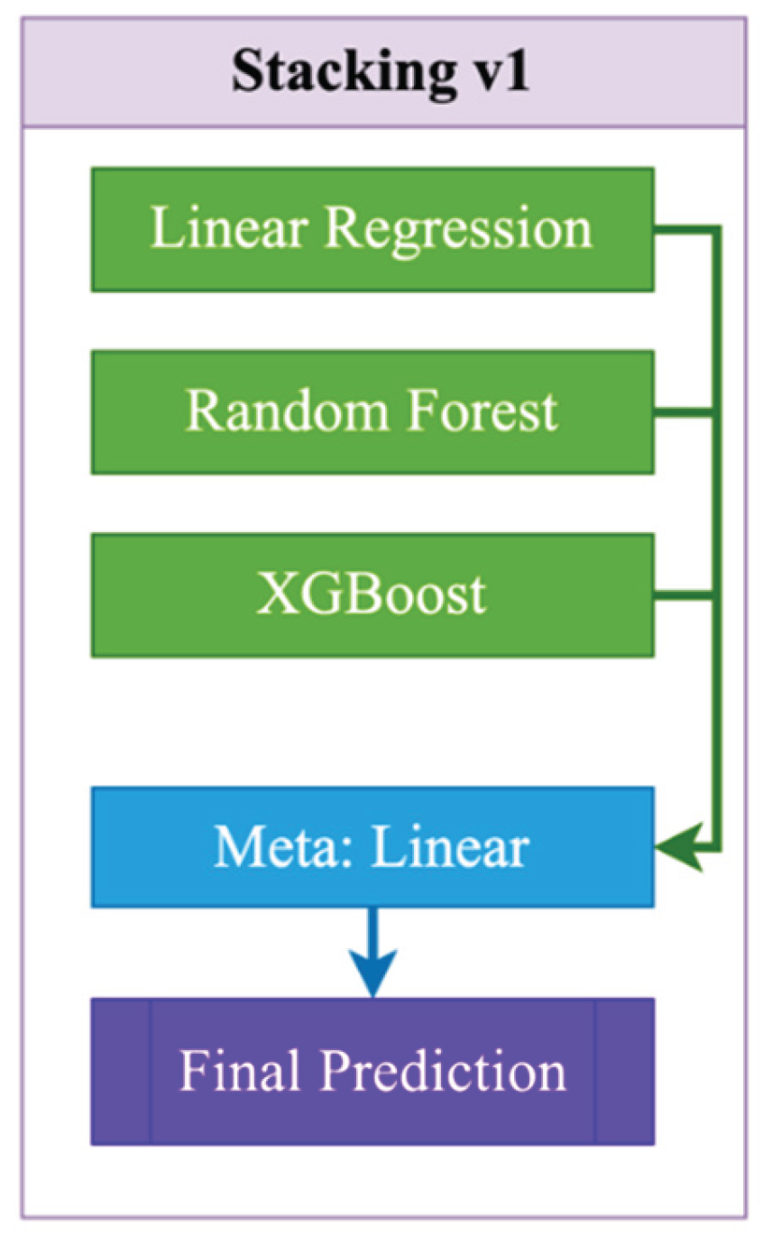
Figure 2.
Stacking v2 architecture.
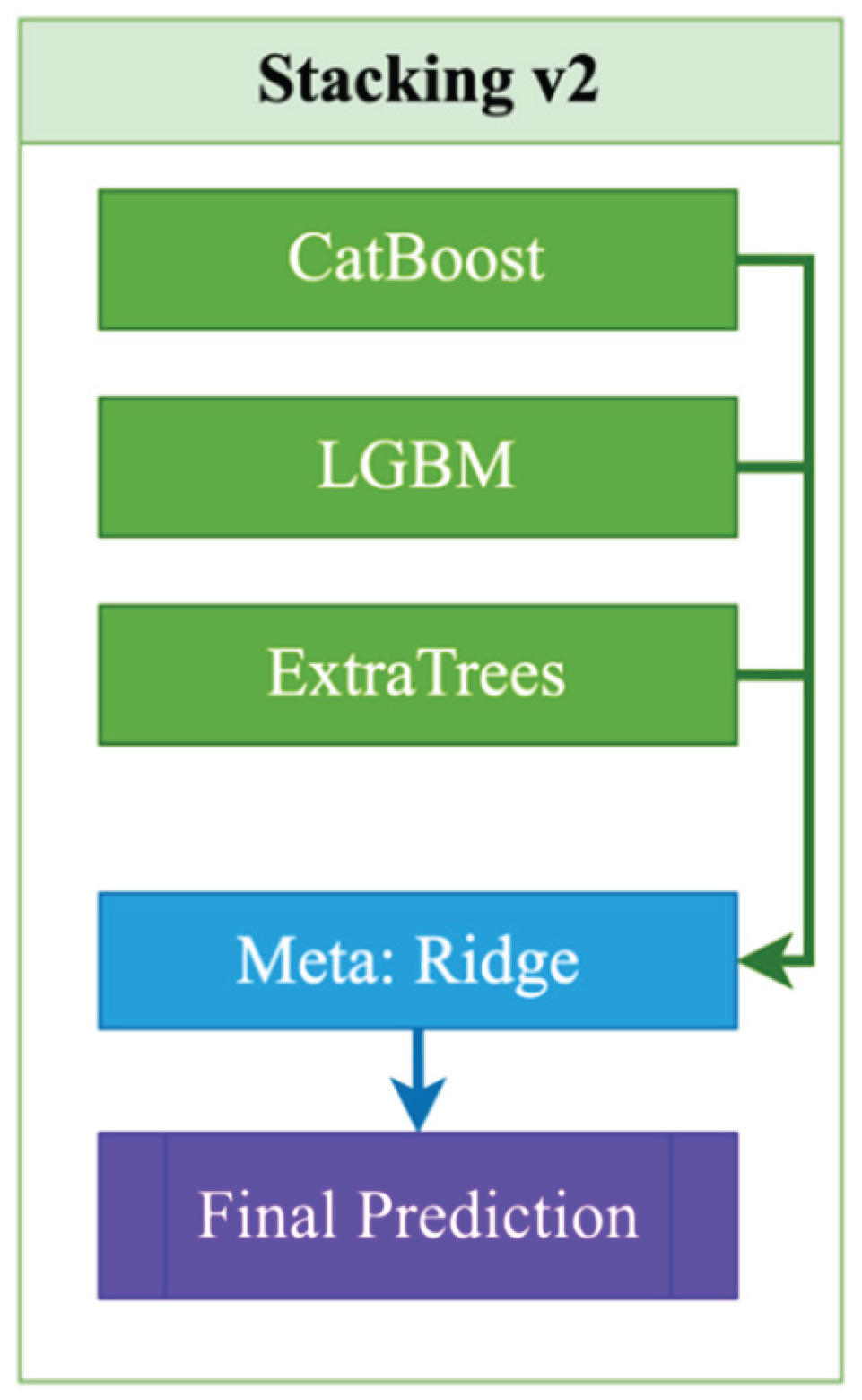
Figure 3.
Stacking v3 architecture.
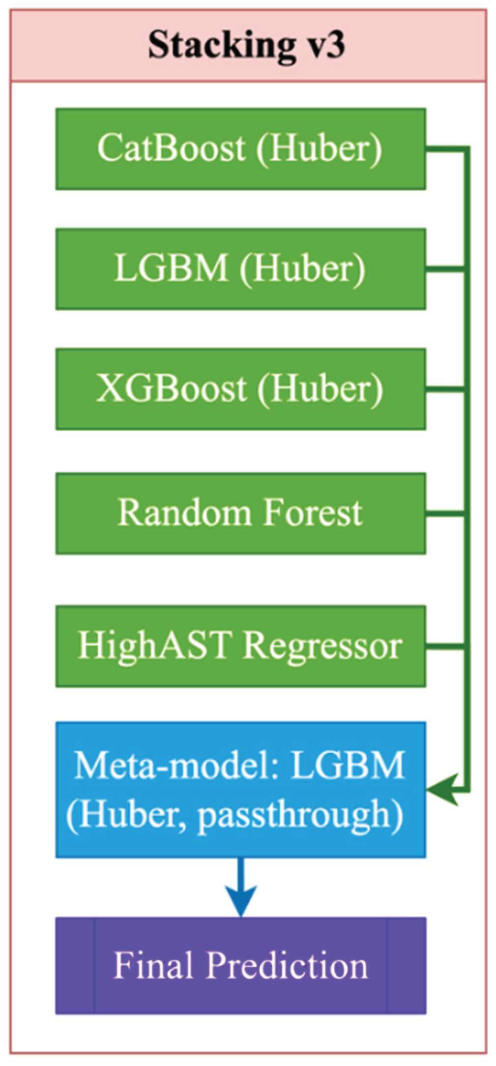
Figure 4.
An algorithm for constructing a prognostic model for aspartate aminotransferase (AST) levels.
Figure 4.
An algorithm for constructing a prognostic model for aspartate aminotransferase (AST) levels.
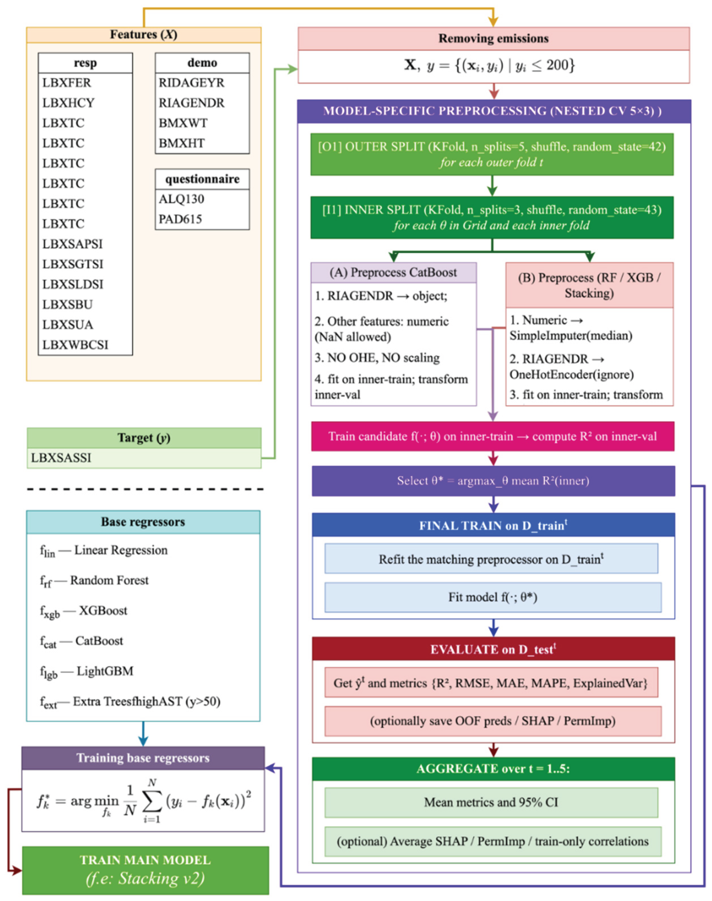
Figure 5.
Comparison of R² scores between full feature set and feature set without GGT/LDH for various models.
Figure 5.
Comparison of R² scores between full feature set and feature set without GGT/LDH for various models.
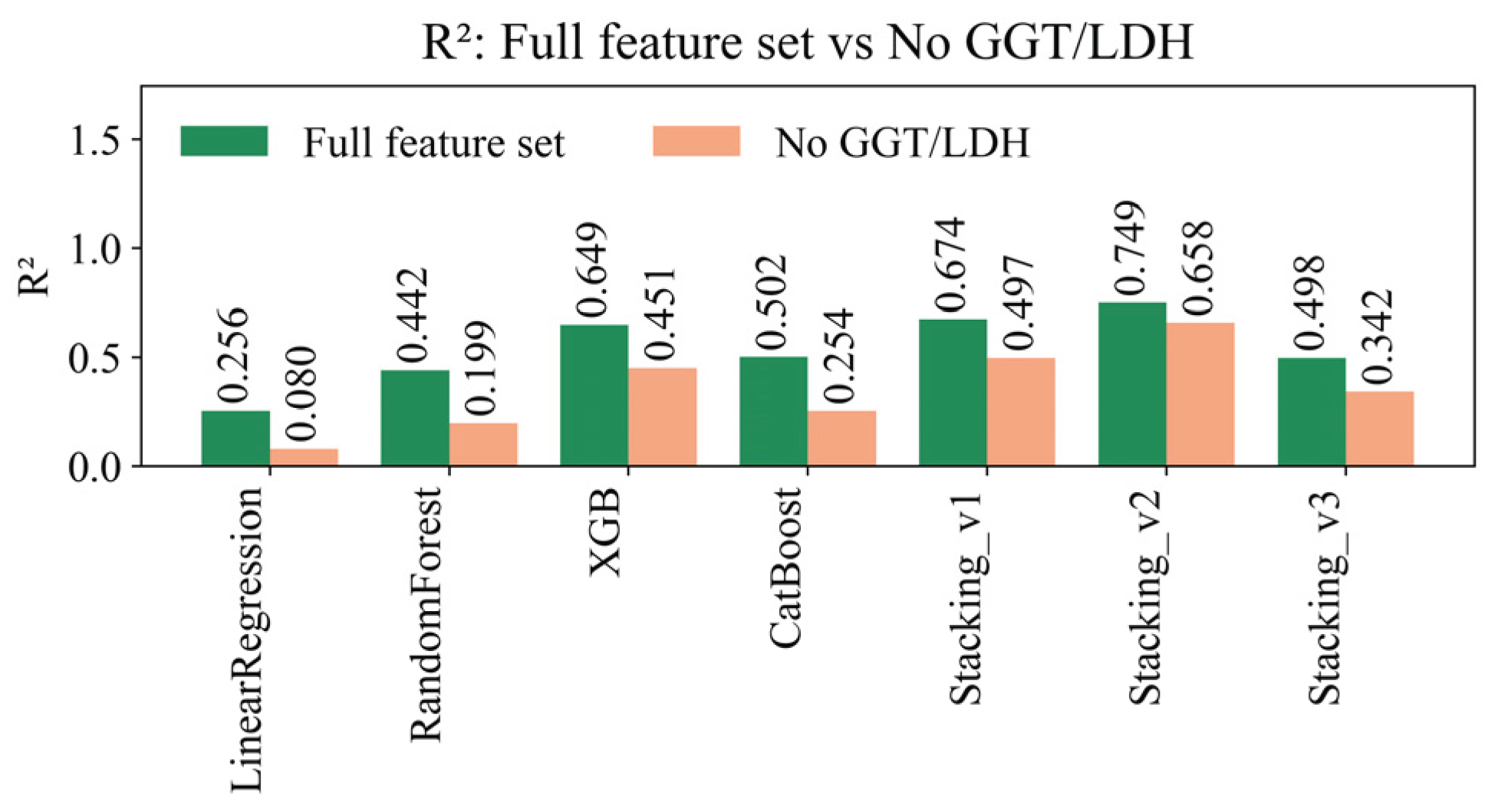
Figure 6.
RMSE comparison between full feature set and reduced set without GGT/LDH across models.
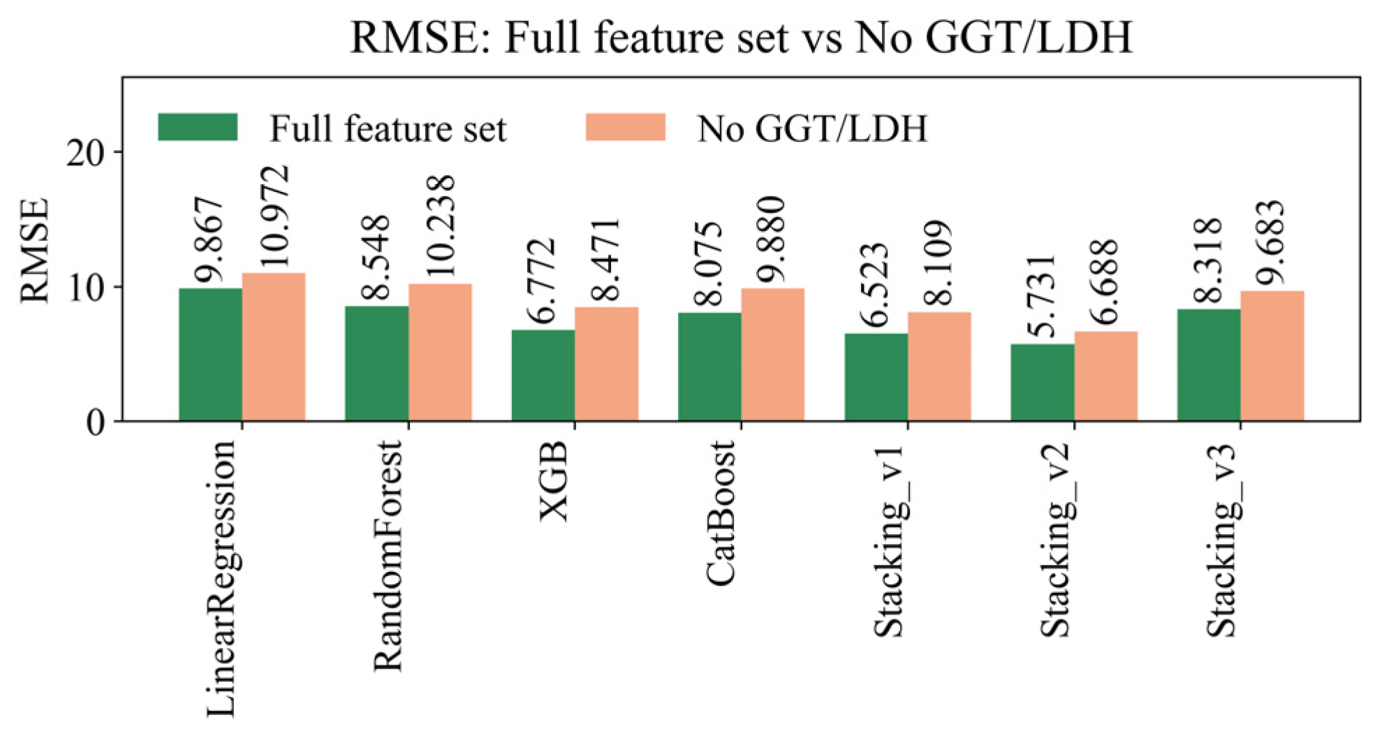
Figure 7.
Comparison of MAE for full feature set and exclusion of GGT/LDH across various regression models.
Figure 7.
Comparison of MAE for full feature set and exclusion of GGT/LDH across various regression models.
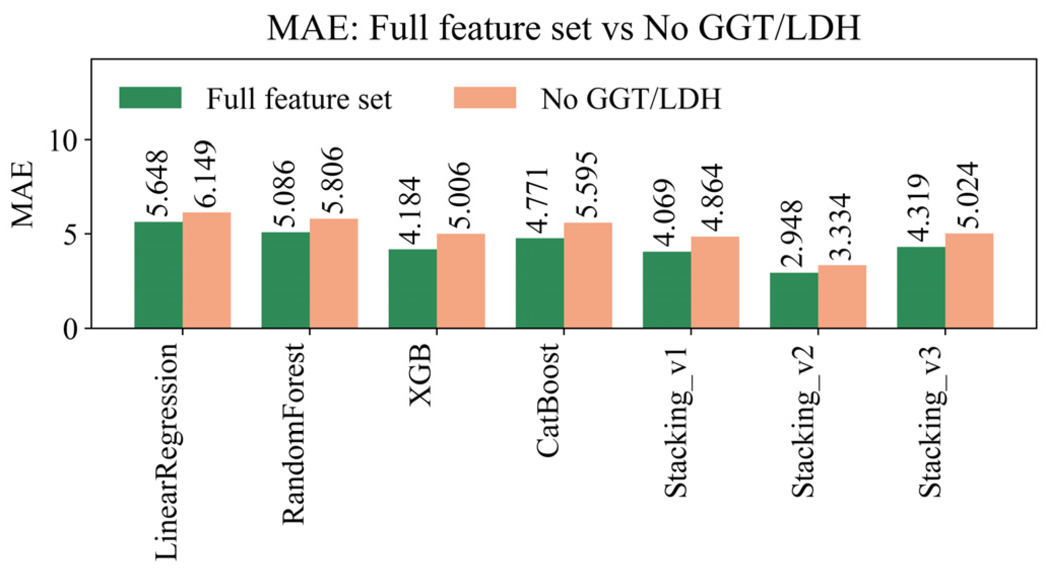
Figure 8.
Comparison of MAPE for full feature set and exclusion of GGT/LDH across various regression models.
Figure 8.
Comparison of MAPE for full feature set and exclusion of GGT/LDH across various regression models.
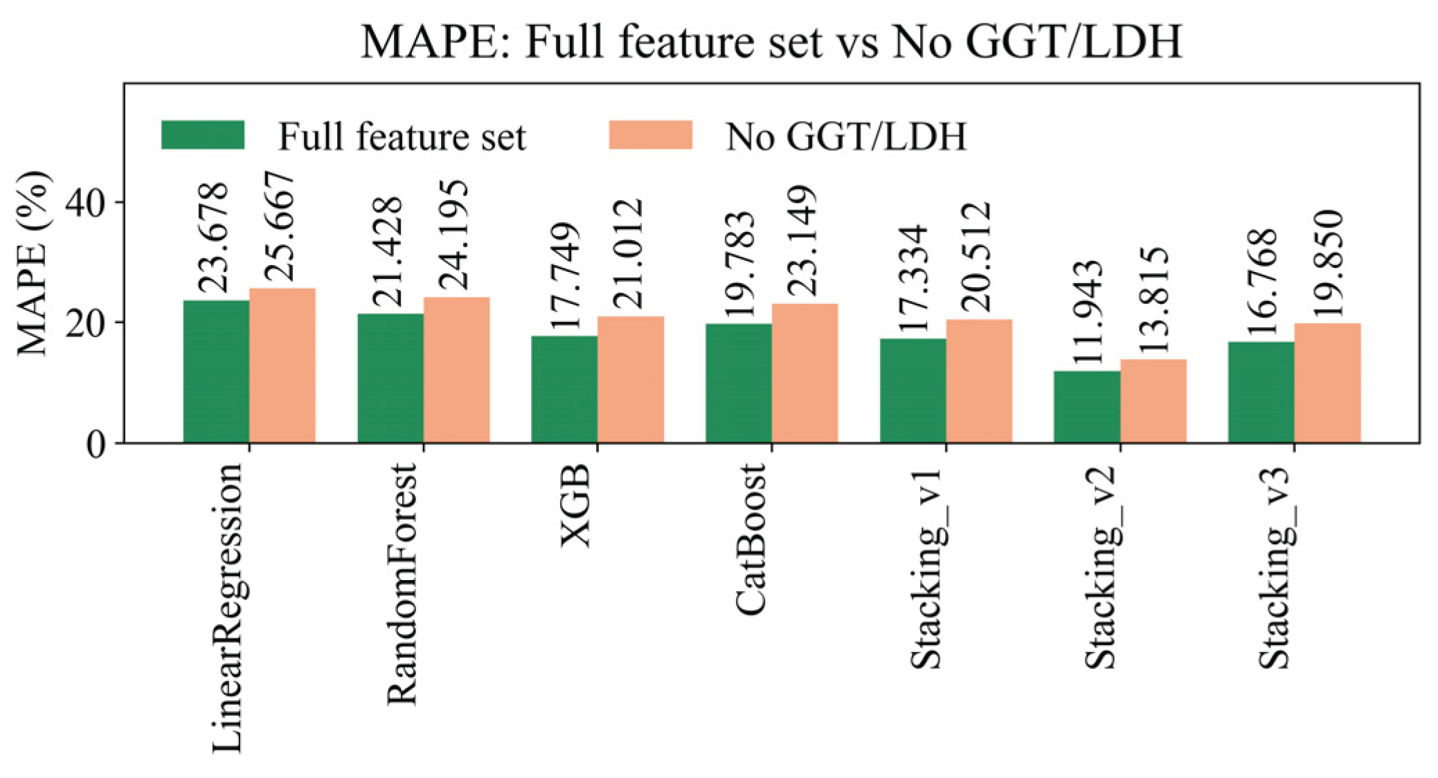
Figure 9.
Comparison of EV across models with full feature set and without GGT/LDH.
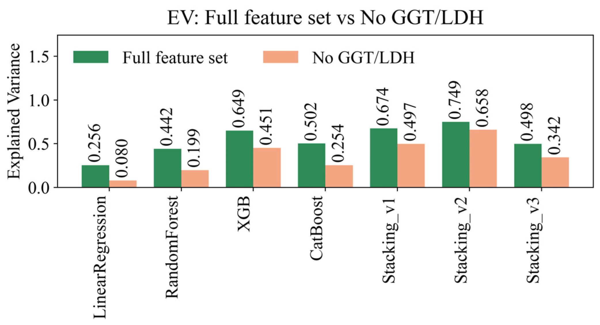
Figure 10.
Contribution of each feature to the prediction of the AST level using different methods (SHAP, Mutual Info, correlations).
Figure 10.
Contribution of each feature to the prediction of the AST level using different methods (SHAP, Mutual Info, correlations).
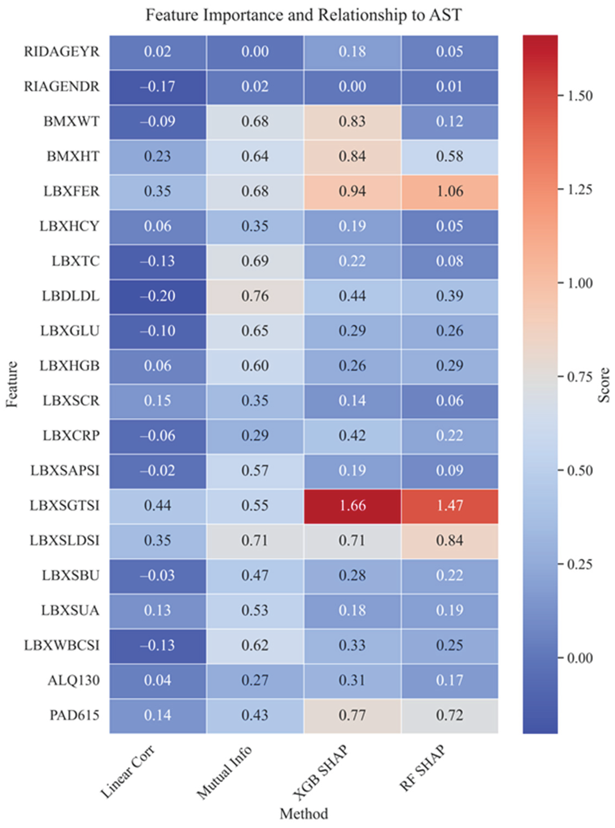
Figure 11.
SHAP Beeswarm - the contribution of each feature and the influence of values on the AST prediction.
Figure 11.
SHAP Beeswarm - the contribution of each feature and the influence of values on the AST prediction.
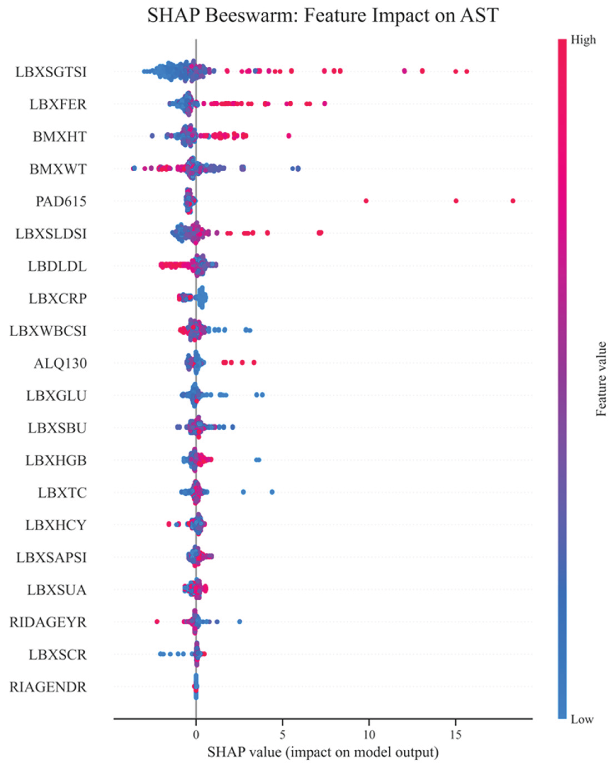
Figure 12.
Ranking features by mean absolute SHAP (XGBoost).
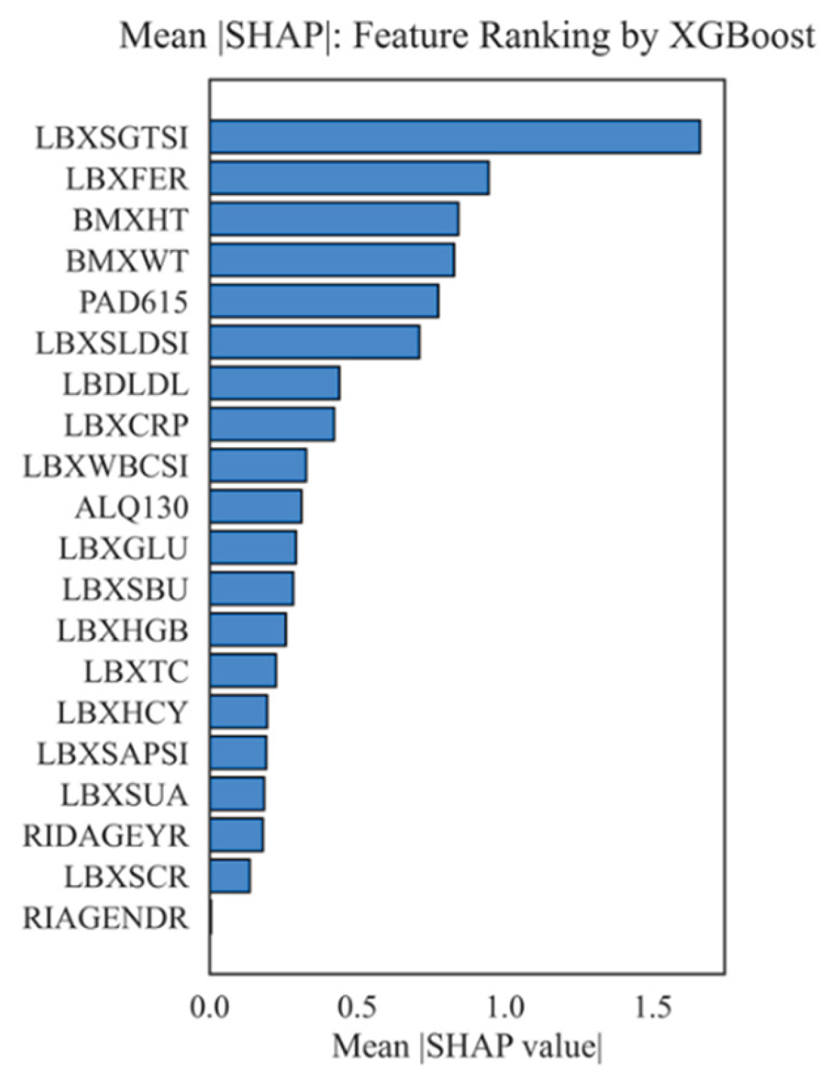
Figure 13.
Top 10 feature pairs with maximum interactions (SHAP interactions).
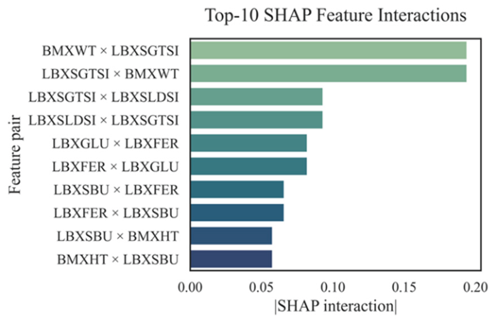
Figure 14.
Matrix of robust correlations between AST and biochemical markers.
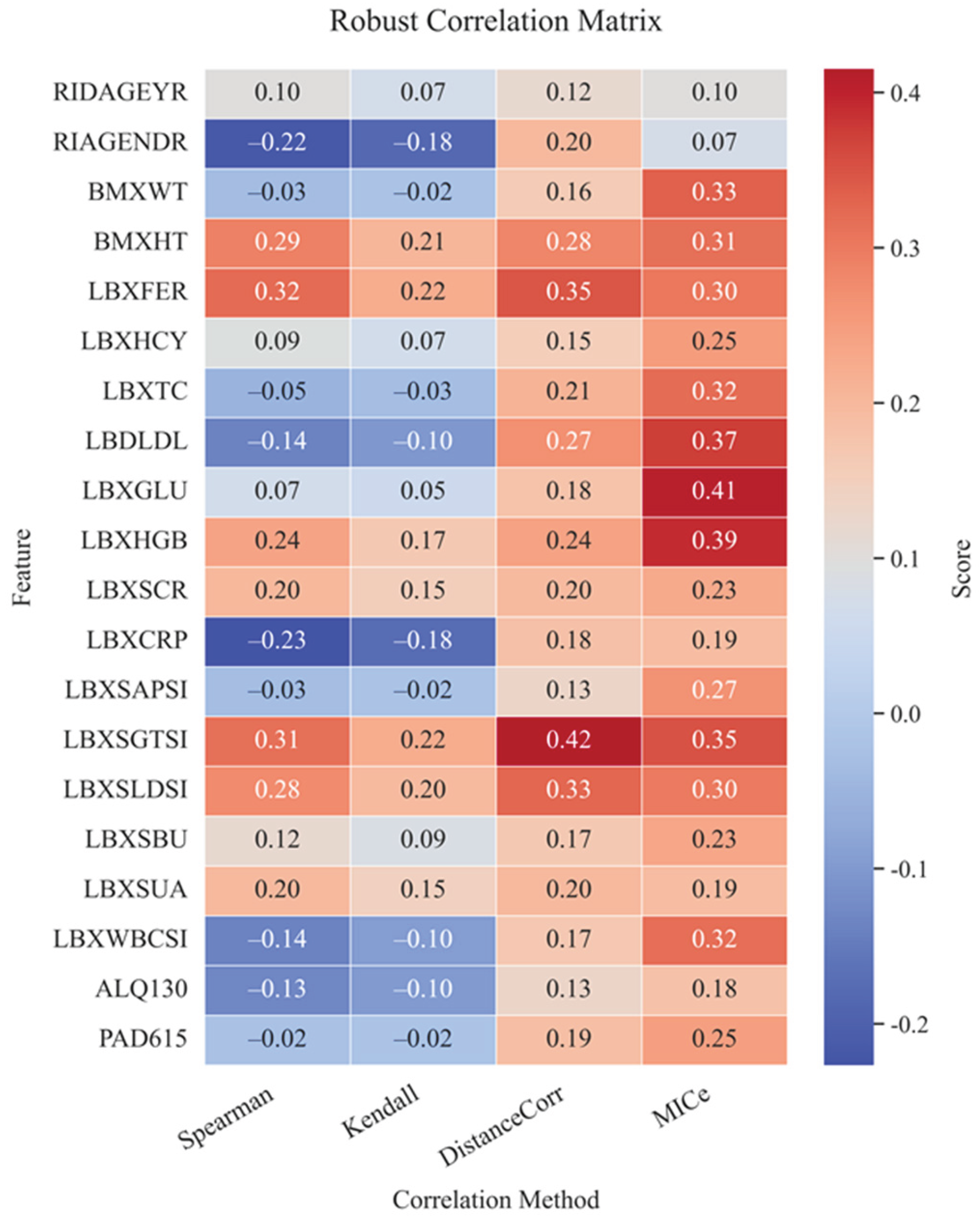
Figure 15.
Cluster structure of features and their grouping by similarity of contribution to AST.
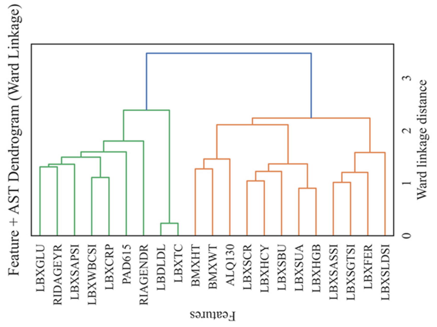
Figure 16.
Calibration of the LGBM model by prediction quantiles.
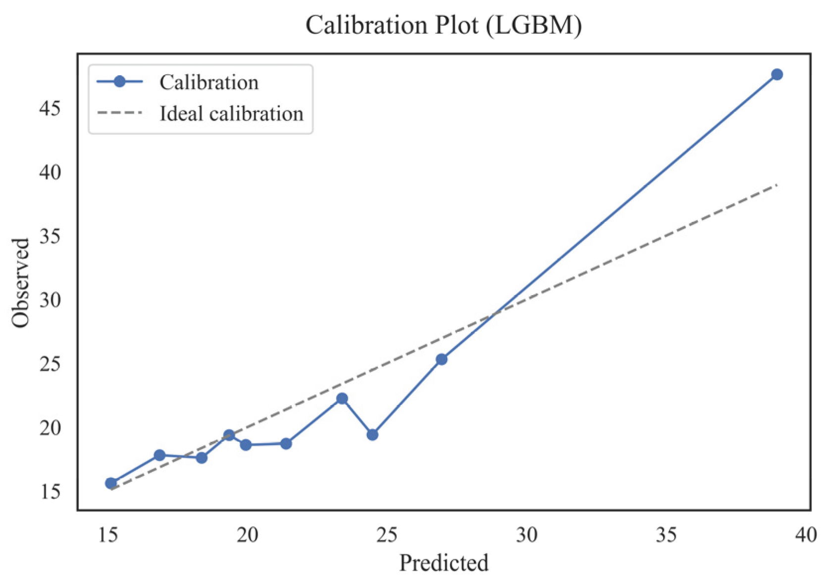
Figure 17.
Calibration comparison across models.
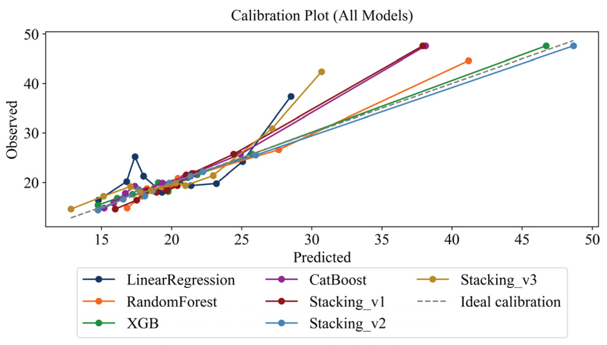
Figure 18.
ROC curve (AUC=1.000) – ability to identify patients with elevated AST.
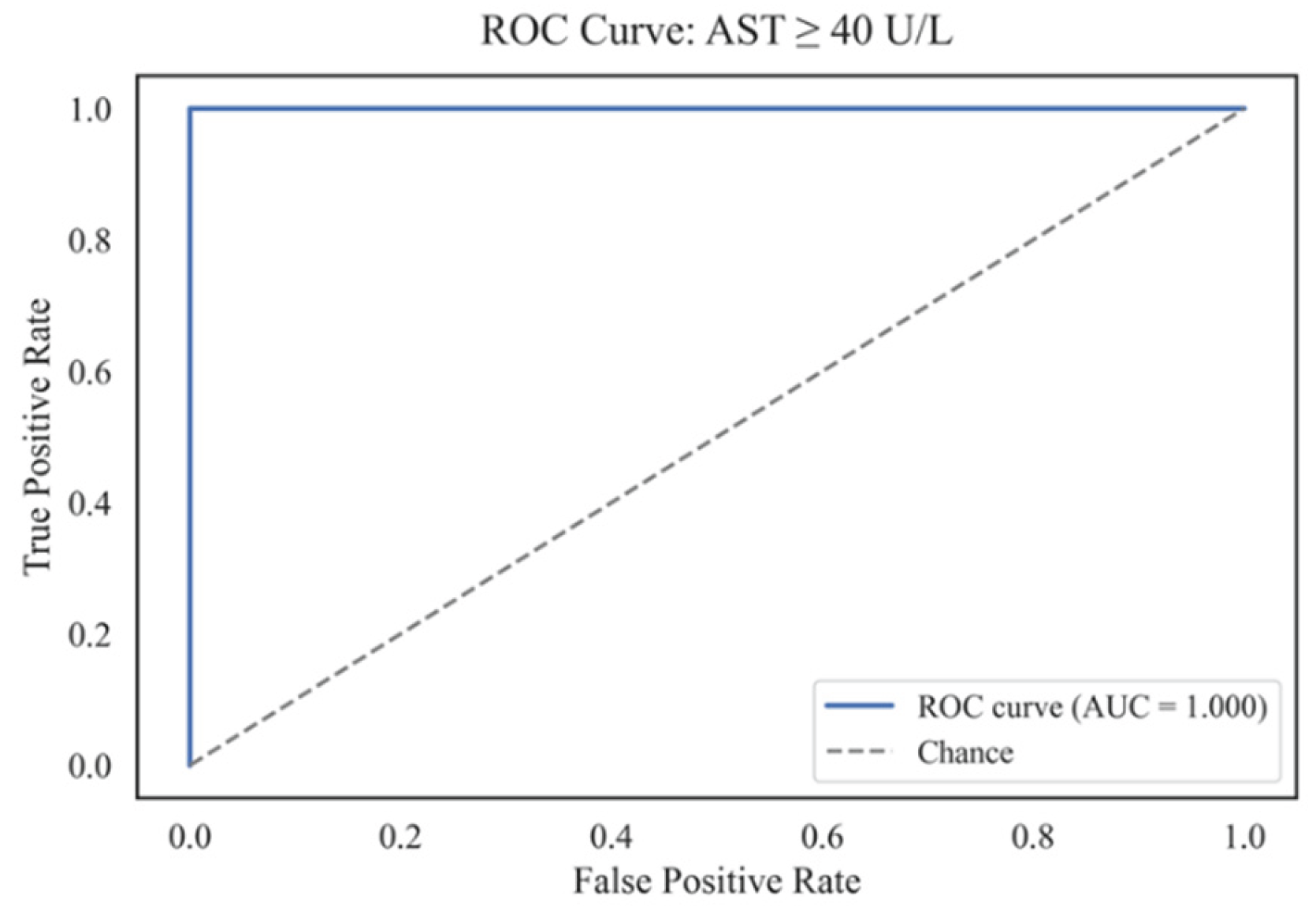
Figure 19.
Precision-Recall-curve (AP=1.000).
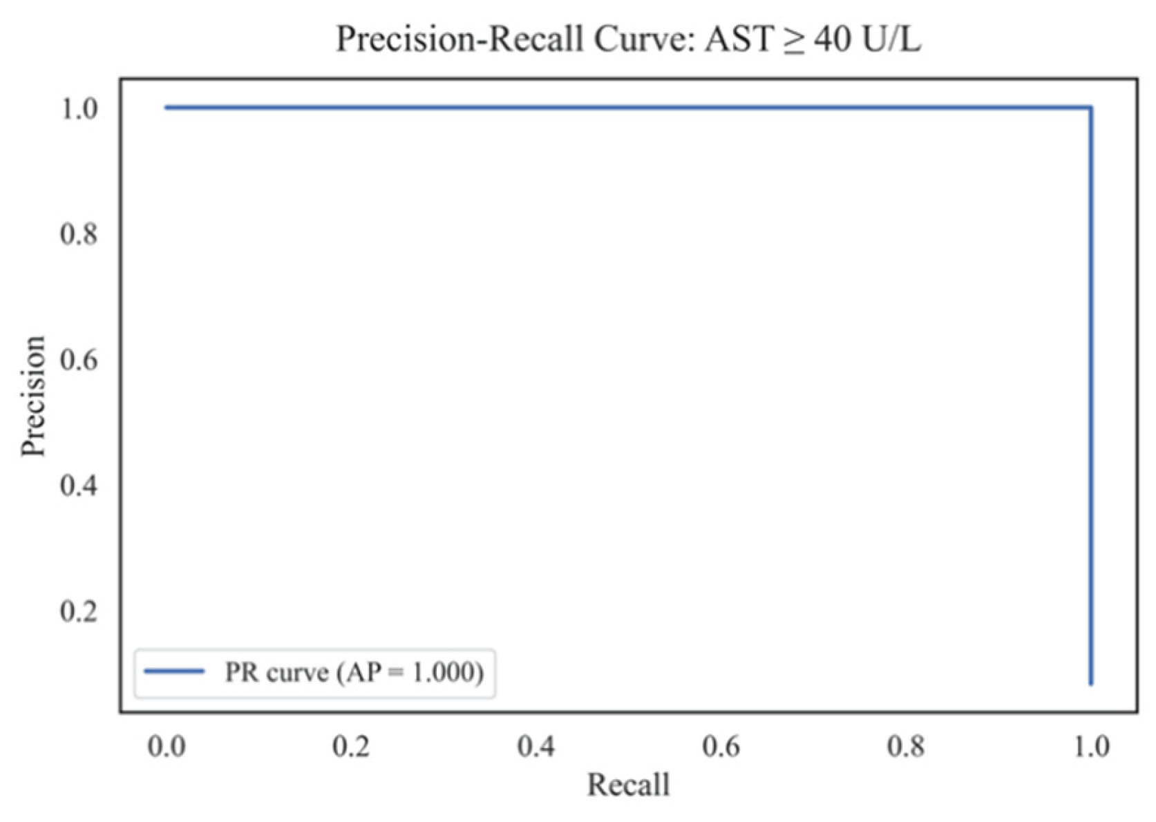
Figure 20.
Confusion matrices for all classification models.
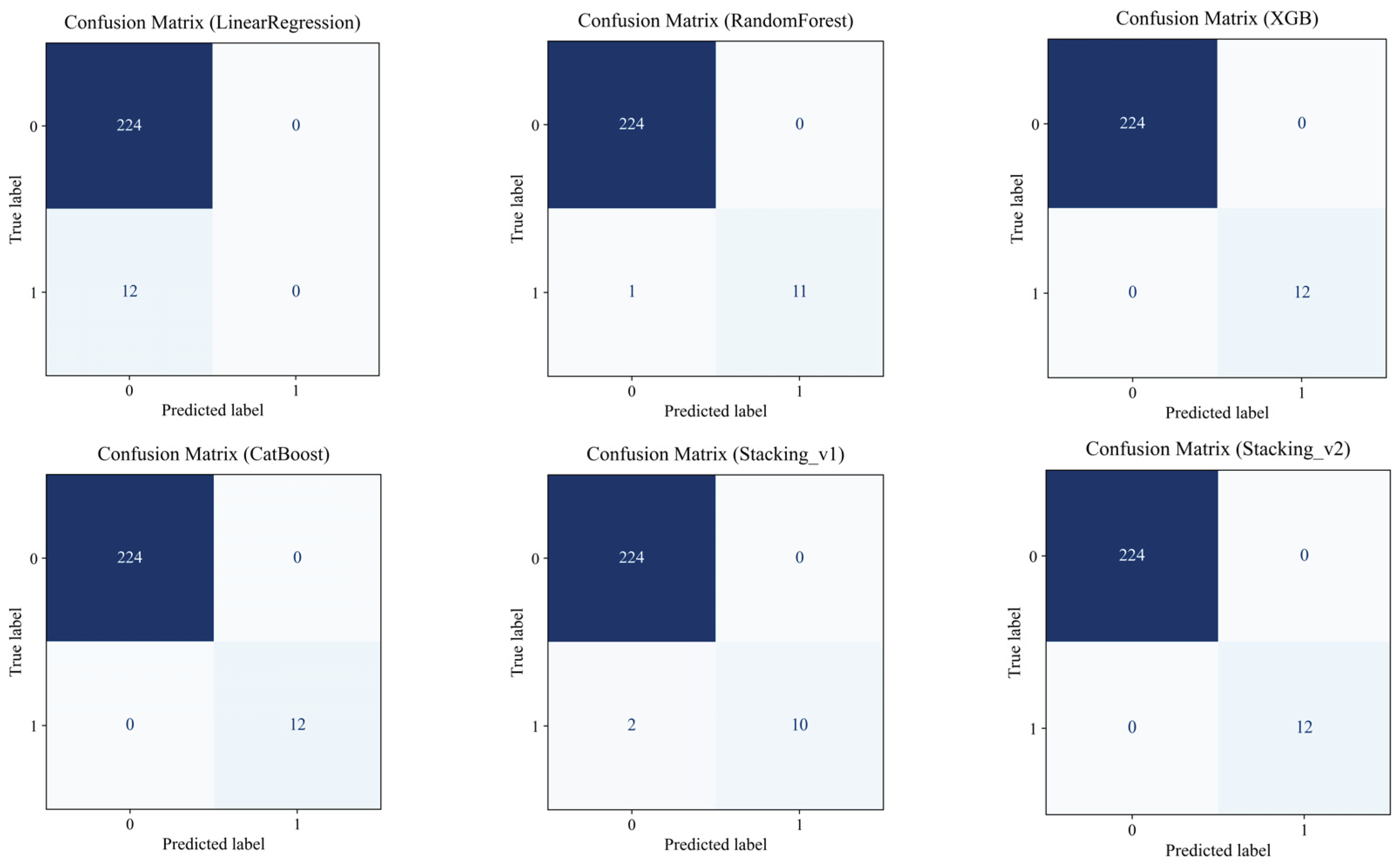
Table 1.
Comparative review of studies on the application of machine learning methods for disease prediction associated with biomarkers (including AST).
Table 1.
Comparative review of studies on the application of machine learning methods for disease prediction associated with biomarkers (including AST).
| Ref. | Study Focus | Methods | Key Findings | Identified Gaps |
|---|---|---|---|---|
| [16] | Predicting liver enzyme elevation in RA patients on methotrexate | Random Forest classifier on EHR data | The ML model accurately predicts transaminase elevation | Specific to RA patients, limited generalizability |
| [17] | ML models for MASLD prediction using demographic and clinical data | Comparison of 10 ML algorithms, including XGBoost and Random Forest | High accuracy in MASLD screening; accessible features | Did not focus on AST-specific prediction |
| [18] | ML with SHAP for NAFLD prediction | ML models with SHAP interpretability | Robust predictive tool for NAFLD; high accuracy and generalizability | Lacks longitudinal data and lifestyle factors |
| [19] | ML models for cardiovascular disease diagnosis using routine blood tests | Logistic Regression, Random Forest, SVM, XGBoost, DNN | Effective diagnosis using accessible blood data; SHAP for interpretation | Focused on cardiovascular diseases, not liver-specific |
| [20] | ML models in liver transplantation prognostication | A systematic review of ML applications | ML models outperform traditional scoring systems in predicting post-transplant complications. | Emphasis on transplantation, not general AST prediction |
| [21] | Early liver disease prediction using deep learning | Deep learning algorithms | A promising approach for rapid and accurate liver disease diagnosis | Requires further validation and integration into clinical practice |
| [22] | Comparison of ML models for liver disease detection using big data | Evaluation of three ML models on 32,000 records | Enhanced prediction and management of liver diseases | Specific models and features are not detailed |
| [23] | ML model to predict liver-related outcomes post-hepatitis B cure | ML-based risk prediction model | Accurate forecasting of liver-related outcomes after functional cure | Focused on hepatitis B, not general AST prediction |
| [24] | Comparative analysis of ensemble learning techniques for fatigue life prediction | Boosting, stacking, bagging vs. linear regression and KNN | Ensemble models outperform traditional methods in prediction tasks | Application in fatigue life; relevance to AST prediction, indirect |
Table 2.
Models and key hyperparameters used in the experiments (nested-CV 5x3 scheme).
| Model | Type/Role | Key Settings |
|---|---|---|
| Linear Regression | Basic reference point | fit_intercept=True |
| Random Forest | Ensemble of trees | n_estimators=300, max_depth=8, random_state=42 |
| XGBoost | Gradient Boosting | n_estimators=300, max_depth=8, learning_rate=0.05, objective="reg:squarederror", random_state=42 |
| CatBoost | Robust Boosting (Native Categories) | iterations=1200, depth=6, learning_rate=0.03, loss_function ∈ {Huber:δ=2.0, RMSE} — is selected in the internal CV |
| Stacking_v1 | Base: Linear + RF + XGB; meta: LinearRegression | passthrough=False |
| Stacking_v2 | Base: CatBoost + LGBM + ExtraTrees; Meta: Ridge | LGBM(n_estimators=2000, lr=0.015, subsample=0.8, colsample_bytree=0.7, reg_lambda=0.8); ExtraTrees(n_estimators=700, max_features="sqrt", min_samples_leaf=2); Ridge(alpha=1.0) |
| Stacking_v3 | Base: CatBoost(Huber) + LGBM(Huber) + XGB + RF + HighASTRegressor; Meta: LGBM(Huber) | HighASTRegressor: y>50, LGBM(objective="huber", n_estimators=400, num_leaves=32); meta: LGBM(objective="huber", n_estimators=400, num_leaves=32), passthrough=True |
Table 3.
Summary statistics for variables used in the final dataset (after filtering and merging).
| Variable | N | Min | 25% | Median | 75% | Max | IQR |
|---|---|---|---|---|---|---|---|
| RIDAGEYR | 201 850 | 0.00 | 17.00 | 34.00 | 57.00 | 90.00 | 40.00 |
| RIAGENDR | 201 850 | 1.00 | 1.00 | 2.00 | 2.00 | 2.00 | 1.00 |
| BMXWT | 199 811 | 21.80 | 61.20 | 72.90 | 86.50 | 371.00 | 25.30 |
| BMXHT | 200 050 | 118.50 | 159.00 | 166.00 | 173.50 | 206.50 | 14.50 |
| LBXFER | 145 110 | 1.04 | 28.40 | 61.00 | 133.00 | 3 234.00 | 104.60 |
| LBXHCY | 99 679 | 1.65 | 6.00 | 7.67 | 9.87 | 156.30 | 3.87 |
| LBXTC | 201 601 | 59.00 | 161.00 | 188.00 | 220.00 | 813.00 | 59.00 |
| LBDLDL | 89 515 | 9.00 | 88.00 | 111.00 | 138.00 | 629.00 | 50.00 |
| LBXGLU | 123 350 | 21.00 | 89.30 | 97.00 | 109.30 | 686.20 | 20.00 |
| LBXHGB | 200 863 | 4.95 | 13.00 | 14.02 | 15.10 | 19.90 | 2.10 |
| LBXSCR | 201 844 | 0.10 | 0.70 | 0.90 | 1.10 | 17.80 | 0.40 |
| LBXCRP | 177 089 | 0.01 | 0.13 | 0.21 | 0.41 | 29.60 | 0.28 |
| LBXSAPSI | 201 841 | 7.00 | 62.00 | 78.00 | 101.00 | 1 378.00 | 39.00 |
| LBXSGTSI | 185 105 | 1.00 | 13.00 | 19.00 | 29.00 | 2 274.00 | 16.00 |
| LBXSLDSI | 201 729 | 4.00 | 122.00 | 141.00 | 166.00 | 1 274.00 | 44.00 |
| LBXSBU | 201 848 | 1.00 | 10.00 | 12.00 | 16.00 | 122.00 | 6.00 |
| LBXSUA | 201 847 | 0.20 | 4.30 | 5.20 | 6.20 | 18.00 | 1.90 |
| LBXWBCSI | 200 867 | 1.40 | 5.70 | 6.90 | 8.40 | 400.00 | 2.70 |
| ALQ130 | 50 467 | 1.00 | 1.00 | 2.00 | 3.00 | 999.00 | 2.00 |
| PAD615 | 9 190 | 10.00 | 60.00 | 120.00 | 240.00 | 9 999.00 | 180.00 |
| LBXSASSI | 201 850 | 6.00 | 18.00 | 21.00 | 26.00 | 200.00 | 8.00 |
Table 4.
Main parameters of the models and the structure of the ensembles.
| Model | Brief Description | Key parameters |
|---|---|---|
| Linear Regression | Basic Interpretable Model | default |
| Random Forest | Decision Tree Ensemble | n_estimators=300, max_depth=8, random_state=42 |
| XGBoost | Gradient Boosting | n_estimators=300, max_depth=8, learning_rate=0.05, objective='reg:squared error, random_state=42 |
| CatBoost | Robust Gradient Boosting | iterations=1200, depth=6, learning_rate=0.03, loss_function='Huber:delta=2.0', random_state=42 |
| Stacking_v1 | Linear + RF + XGBoost | meta=Linear Regression |
| Stacking_v2 | CatBoost + LGBM + ExtraTrees | meta=Ridge Regression (alpha=1.0) |
| Stacking_v3 | CatBoost + LGBM + XGB + RF + high_AST | meta=LGBM (huber), passthrough=True, регрессoр “high_AST”: LGBM (objective='huber', n_estimators=400) |
| Advanced Stacking | Specialized regressor for high_AST | LGBM (separately on the subsample with high AST) |
Table 5.
Performance metrics of regression models using 5-fold cross-validation on the full feature set.
Table 5.
Performance metrics of regression models using 5-fold cross-validation on the full feature set.
| Metric | LinearRegression | RandomForest | XGB | CatBoost | Stacking_v1 | Stacking_v2 | Stacking_v3 |
|---|---|---|---|---|---|---|---|
| R2 (mean) | 0.215 | 0.629 | 0.728 | 0.759 | 0.690 | 0.916 | 0.612 |
| R2 (std) | 0.285 | 0.253 | 0.360 | 0.135 | 0.333 | 0.143 | 0.087 |
| RMSE (mean) | 6.813 | 4.389 | 3.234 | 3.648 | 3.668 | 2.274 | 5.150 |
| RMSE (std) | 0.976 | 1.084 | 1.898 | 0.832 | 1.675 | 0.925 | 1.634 |
| MAE (mean) | 4.923 | 3.198 | 1.369 | 1.916 | 2.241 | 1.303 | 2.779 |
| MAE (std) | 0.562 | 0.673 | 0.807 | 0.381 | 0.881 | 0.507 | 0.601 |
| MAPE (mean) | 22.96 | 15.14 | 6.47 | 8.26 | 10.72 | 6.564 | 10.84 |
| MAPE (std) | 2.02 | 3.67 | 4.18 | 2.01 | 4.89 | 2.863 | 1.77 |
| ExplainedVar (mean) | 0.217 | 0.659 | 0.744 | 0.771 | 0.716 | 0.926 | 0.633 |
| ExplainedVar (std) | 0.285 | 0.233 | 0.331 | 0.136 | 0.290 | 0.097 | 0.087 |
Table 6.
Comparison of model quality by Nested CV (mean±95% CI).
| Model | R² (±95% CI) | RMSE (±95% CI) | MAE (±95% CI) | MAPE (±95% CI) | EV (±95% CI) |
|---|---|---|---|---|---|
| LinearRegression | 0.2558 ± 0.0128 | 9.8675 ± 0.2617 | 5.6477 ± 0.0506 | 23.6785 ± 0.0871 | 0.2559 ± 0.0128 |
| RandomForest | 0.4416 ± 0.0075 | 8.5477 ± 0.2190 | 5.0857 ± 0.0524 | 21.4277 ± 0.1158 | 0.4416 ± 0.0075 |
| XGBoost | 0.6492 ± 0.0143 | 6.7716 ± 0.1559 | 4.1842 ± 0.0451 | 17.7494 ± 0.1199 | 0.6492 ± 0.0143 |
| CatBoost | 0.5017 ± 0.0071 | 8.0747 ± 0.2146 | 4.7712 ± 0.0474 | 19.7826 ± 0.1306 | 0.5017 ± 0.0071 |
| Stacking_v1 | 0.6743 ± 0.0174 | 6.5227 ± 0.1365 | 4.0688 ± 0.0450 | 17.3341 ± 0.1131 | 0.6743 ± 0.0174 |
| Stacking_v2 | 0.7491 ± 0.0065 | 5.7307 ± 0.2088 | 2.9480 ± 0.0396 | 11.9428 ± 0.0857 | 0.7491 ± 0.0065 |
| Stacking_v3 | 0.4982 ± 0.0041 | 8.318 ± 0.0490 | 4.319 ± 0.0176 | 16.768 ± 0.0407 | 0.4982 ± 0.0041 |
Table 7.
Results of mediator analysis of the influence of biomarkers and lifestyle factors on aspartate aminotransferase (AST) levels.
Table 7.
Results of mediator analysis of the influence of biomarkers and lifestyle factors on aspartate aminotransferase (AST) levels.
| Mediator | Path | Coef. | SE | p-Value | 95% CI (Low) | 95% CI (Upper) | Significance | Description of the Effect |
|---|---|---|---|---|---|---|---|---|
| LBXFER Ferritin |
Direct | 0.0231 | 0.0040 | 1.20e-8 | 0.0155 | 0.0309 | Yes | Major contribution via direct path (significant) |
| Indirect | -0.0003 | 0.0010 | 0.672 | -0.0026 | 0.0013 | No | The indirect effect is not significant. | |
| Total | 0.0229 | 0.0040 | 3.58e-8 | 0.0150 | 0.0309 | Yes | The overall effect remains | |
| LBXSGTSI Gamma-GT |
Direct | 0.0138 | 0.0041 | 9.42e-4 | 0.0057 | 0.0218 | Yes | Significant direct influence |
| Indirect | 0.0092 | 0.0027 | 0.000 | 0.0047 | 0.0154 | Yes | The indirect effect is statistically significant. | |
| Total | 0.0229 | 0.0040 | 3.58e-8 | 0.0150 | 0.0309 | Yes | Overall mediation effect | |
| BMXHT Height (cm) |
Direct | 0.0201 | 0.0042 | 2.55e-6 | 0.0119 | 0.0284 | Yes | Significant direct path |
| Indirect | 0.0028 | 0.0019 | 0.008 | 0.0004 | 0.0078 | Yes | The indirect effect is significant. | |
| Total | 0.0229 | 0.0040 | 3.58e-8 | 0.0150 | 0.0309 | Yes | The overall effect is maintained | |
| LBXSBU Urea (BUN) |
Direct | 0.0262 | 0.0042 | 1.97e-9 | 0.0179 | 0.0345 | Yes | The main effect is direct. |
| Indirect | -0.0033 | 0.0015 | 0.000 | -0.0071 | -0.0013 | Yes | The indirect effect is statistically significant. | |
| Total | 0.0229 | 0.0040 | 3.58e-8 | 0.0150 | 0.0309 | Yes | The final effect is confirmed | |
| LBXGLU Fasting glucose |
Direct | 0.0241 | 0.0040 | 7.70e-9 | 0.0162 | 0.0320 | Yes | The direct effect is clearly expressed. |
| Indirect | -0.0011 | 0.0007 | 0.008 | -0.0035 | -0.0002 | Yes | The indirect effect is expressed. | |
| Total | 0.0229 | 0.0040 | 3.58e-8 | 0.0150 | 0.0309 | Yes | The overall effect is confirmed | |
| LBXSLDSI |
Direct | 0.0198 | 0.0039 | 6.32e-7 | 0.0122 | 0.0274 | Yes | Significant direct contribution |
| Indirect | 0.0031 | 0.0019 | 0.004 | 0.0009 | 0.0082 | Yes | The indirect effect is statistically significant. | |
| Total | 0.0229 | 0.0040 | 3.58e-8 | 0.0150 | 0.0309 | Yes | The overall effect is expressed | |
| PAD615 activity in min | Direct | 0.0238 | 0.0040 | 8.59e-9 | 0.0159 | 0.0316 | Yes | The main contribution is direct. |
| Indirect | -0.0008 | 0.0008 | 0.240 | -0.0030 | 0.0003 | No | The indirect effect is insignificant. | |
| Total | 0.0229 | 0.0040 | 3.58e-8 | 0.0150 | 0.0309 | Yes | The final effect is confirmed. |
Disclaimer/Publisher’s Note: The statements, opinions and data contained in all publications are solely those of the individual author(s) and contributor(s) and not of MDPI and/or the editor(s). MDPI and/or the editor(s) disclaim responsibility for any injury to people or property resulting from any ideas, methods, instructions or products referred to in the content. |
© 2025 by the authors. Licensee MDPI, Basel, Switzerland. This article is an open access article distributed under the terms and conditions of the Creative Commons Attribution (CC BY) license (http://creativecommons.org/licenses/by/4.0/).
Copyright: This open access article is published under a Creative Commons CC BY 4.0 license, which permit the free download, distribution, and reuse, provided that the author and preprint are cited in any reuse.


