Submitted:
13 November 2025
Posted:
18 November 2025
You are already at the latest version
Abstract
Forest resources are among the most important ecosystems on the earth. The semantic segmentation and accurate positioning of ground objects in forest remote sensing (RS) imagery are crucial to the emergency treatment of forest natural disasters, especially forest fires. Currently, most existing methods for image semantic segmentation are built upon convolutional neural network (CNN). Nevertheless, these techniques face difficulties in directly accessing global contextual information and accurately detecting geometric transformations within the image’s target regions. This limitation stems from the inherent locality of convolution operations, which are restricted to processing data structured in Euclidean space and confined to square-shaped regions.Inspired by the Graph Convolution Network (GCN) with robust capabilities in processing irregular and complex targets, as well as Swin Transformers renowned for exceptional global context modeling, we present an innovative semantic segmentation framework for forest remote sensing imagery termed GSwin-Unet. This framework embeds GCN model into Swin-Unet architecture, and for the first time apply the method of combining GCN and Transformer in the domain of forest RS imagery analysis. GSwin-Unet features an innovative parallel dual-encoder architecture of GCN and Swin transformer. First, we integrate the Zero-DCE (Zero-Reference Deep Curve Estimation) algorithm into GSwin-Unet to enhance forest RS image feature representation. Second, a feature aggregation module (FAM) is proposed to bridge the dual encoders by fusing GCN-derived local aggregated features with Swin transformer-extracted features. Our study demonstrates that the GSwin-Unet significantly improves performance on the Forest Remote Sensing Dataset and exhibits good adaptability on GID dataset.
Keywords:
forest remote sensing
; graph convolutional network (GCN)
; semantic segmentation
; feature aggregation
1. Introduction
With the rapid advances in sensor and satellite remote sensing technologies, researchers can now readily obtain vast quantities of high-quality forest RS images, which not only reflect the status of forest ecological environments but also detect the natural disasters. Effectively filtering the information of interest and extracting knowledge from these images can offer robust support for the management of forest resource and the prevention and control of forest disasters such as fires, pests and diseases, and meteorological disasters. Semantic segmentation, a technique that classifies individual pixels in an image into distinct semantic classes, has garnered significant interest in the field of remote and computer vision.
In recent years, the rapid advancement of deep learning has catalyzed significant proress in semantic image segmentation. In particular, convolutional neural networks (CNNs) with an encoder-decoder architecture have played a vital role. For instance, the U-shaped network (UNet) [1] employs a decoder to capture spatial dependencies from corresponding encoding stages via skip connections. In this context, Transformer exhibits unique advantages and has emerged as a predominant backbone architectures in semantic image segmentation, particularly in medical imaging applications [2,3,4,5,6,7,8]. The self-attention mechanism confers upon the model an enhanced capacity to capture long-range contextual dependencies, thereby demonstrating the distinct advantages in feature extraction and capturing global image features. For example, SegFormer [9] introduces a hierarchical Transformer architecture that facilitates the concurrent extraction of high-resolution shallow features and low-resolution semantically rich features. Similarly, Swin-Unet employs a shifted-window Swin transformer as its contextual feature extraction encoder, paired with a symmetric decoder with Swin transformer backbone to progressively upsample feature maps.
Forest remote sensing images typically have rich texture features and complex interlaced scenes, with various categories embedded within each other, lacking fixed geometric shapes and clear boundaries. The particularities of forest ground objects —such as low brightness, small scale, mutual occlusion, and high similarity—pose challenges to semantic segmentation for forest RS images, as illustrated in Figure 1. The low brightness in forest RS images, caused by shadow effects, results in lower contrast of ground objects, often leading to semantic ambiguity.
CNNs demonstrate superiority in efficient local perception, however, they struggle to directly model contextual information and global semantic interactions due to the inherent locality of convolution operation [10]. Existing advanced networks [10,11,12,13,14,15] typically aggregate global information from locally extracted CNN features, rather than encoding global context directly. Consequently, this indirect paradigm hinders the acquisition of clear global scene information in RS images with complex backgrounds [16]. Transformer provides a completely new approach for modeling global relationships [17]. As the first pure Transformer-based encoder for semantic segmentation, SETR [18] abandons convolutional backbones and frames the task as a sequence-to-sequence reconstruction problem. Its strong capability in global context modeling is especially useful for handling long-range dependencies in large-scale images. Mask2Former [19] adopts a mask attention mechanism to dynamically focus on key areas, with strong multitasking adaptability and outstanding performance in complex scene segmentation and video tracking. Swin transformer [20] achieves a balance between performance and efficiency by introducing a layered architecture and sliding window mechanism. TransUNet [10] integrates Transformers and CNNs architectures to synergistically capture global semantics and local details, showing superior performance in medical image segmentation tasks including Computed Tomography (CT) and Magnetic Resonance Imaging (MRI) segmentation. Following the U-Net architectural paradigm, Cao et al. [4] introduced Swin-Unet, which integrates Swin transformer’s hierarchical window attention mechanism with skip connections for multi-scale feature fusion. Swin-Unet has shown superior segmentation performance on medical imaging tasks compared to conventional CNN-based models and Transformer-convolution hybrid approaches, particularly in modeling long-range spatial dependencies while maintaining computational efficiency.
However, Transformer-based models rely on global contextual information to make decisions, which may neglect the importance of local details and easily cause small-scale features to be discarded [10]. Additionally, CNN and Transformer can only be applied to Euclidean spatial data and square regions and cannot capture the geometric variations in the target area of the imagery, resulting in poor capturing ability for the same type of objects with different shapes. In forest remote sensing, ground objects in forest with same semantic categories may have different sizes and shapes, while different categories may exhibit analogous material and spectral properties, thereby impeding accurate discrimination between them. Therefore, more hierarchical details and effective processing capabilities are needed to fuse global and local contextual features for semantic reasoning.
In recent years, Graph Convolutional Networks (GCN) have emerged as a powerful paradigm for extracting local features (e.g., edges and textures) from irregular geometric objects by leveraging graph-structured data. As a deep learning framework, GCN performs convolution operations on graph nodes and their neighborhoods, enabling effective feature aggregation for tasks such as classification, clustering, and prediction. In 2019, Chen et al. [21] pioneered a multi-label image recognition approach that modeled label dependencies through graph structures, demonstrating the potential of GCN in semantic reasoning. Building on this, Jung et al. proposed SGCN [22], which integrated dual graph convolutions—spectral convolution with topology adaptiveness and spatial convolution with weighted node sampling—to capture node semantics in super-pixel graphs. This architectural innovation laid the groundwork for the Vision Graph Neural Network (VIG) [23], which has exhibited remarkable performance in processing complex scenes and irregularly shaped objects. While GCN-based models have achieved significant success in imagery recognition and object detection, their application in RS image segmentation remains underexplored.
In this article, to address the inherent limitations of Transformer in local feature modeling and CNN in handling irregular geometric objects, we propose GSwin-Unet, a novel framework that integrates Graph Convolution into Swin-Unet [4] for forest RS imagery’s semantic segmentation. The architecture adopts a parallel dual-encoder design: Swin transformer serves as the principal encoder, while Graph Convolution acts as an auxiliary encoder to capture geometric irregularities. A dedicated Feature Aggregation Module (FAM) is introduced to establish a unidirectional auxiliary-to-main encoder information propagation mechanism to enable effective feature fusion. This design synergizes the strengths of both modules, enhancing the segmentation of complex forest structures.
The self-learning semantic segmentation form of spectral, texture, and shape features extracted from forest remote sensing images through intelligent algorithms is used to mine the information of land targets, thus providing a good foundation for accurately obtaining the basic ground features distribution of forest ecological area.
2. Related Work
2.1. Vision Transformer
Initially proposed for machine translation [24], the standard Transformer architecture comprises three core components: multi-head self-attention (MSA), layer normalization (LN), and multilayer perceptron (MLP), as schematically shown in Figure 2. MSA is a critical component and enables the establishment of global dependencies between output- and input-sequences.
In 2020, Dosovitskiy et al. proposed the Vision Transformer model [17], which introduced Transformer into the field of computer vision. This model quickly achieved high performance in object classification, semantic segmentation, and instance segmentation, addressing the limitations of Recurrent Neural Network(RNN)’s in parallel computing and CNN’s in effectively learning global feature information. Researchers have since proposed a series of advanced architectures derived from Vision Transformer, including Segmentation Transformer (SETR) [18], Swin-Transformer [20], Visual Pyramid Transformer (PVT) [25], TNT [26], and Swin-Unet [4]. These models have demonstrated outstanding performance in the area of vision, particularly in the field of medical imagery segmentation.
SETR [18] pioneered the application of ViT to semantic segmentaion. The SETR model uses encoder with a pure Transformer architecture to replace CNN, altering the existing semantic segmentation model architecture. The multi-scale attention mechanism facilitates robust capture of long-range dependencies between distant structural regions, which is critical for semantic segmentation spanning the images. However, since transformers did not perform well in capturing low-level details and had computational complexity, many improvements were subsequently made. Wang et al.[25] integrated pyramid structure into ViT (PVT), mimicking CNN’s hierarchical design to generate multi-scale features. By strategically reducing sequence length via patch embedding layers, their approach dynamically adapts computational complexity while preserving feature granularity. Han et al. [26] proposed the TNT (Transformer-iN-Transformer) model, which effectively captures both local and global features through nested Transformer architecture, thereby generating richer representations. Yuan et al. [27] proposed a recursive token aggregation mechanism that progressively merges adjacent tokens to capture hierarchical local structures while reducing computational complexity through token count reduction.
Although the models mentioned above improved the feature capture capability, their complexity remains quadratic with respect to image size, a property that directly impairs training and inference speed when processing large-scale datasets. To mitigate this limitation, Liu et al. [20] developed the Swin transformer, a groundbreaking architecture that employs a shifted window strategy to confine multi-head self-attention (MSA) within local windows while enabling cross-window communication. This approach yields linear computational complexity relative to input size and achieves advanced performance across vision tasks such as image classification, object detection, and semantic segmentation. The Swin transformer replaces standard MSA with Window-based MSA (W-MSA) and Shifted Window-based MSA (SW-MSA) mechanisms, as illustrated in Figure 3. Wang et al. [28] enhanced PVT by introducing a linear-complexity attention mechanism and overlapping patch embedding, which reduced computational complexity from quadratic to linear while maintaining superior performance on fundamental vision tasks. Cao et al. [4] developed specialized U-shaped encoder-decoder architectures based on Swin transformer, optimized for precise segmentation tasks. Lin et al. [29] implemented a dual-encoder framework using Swin transformers with dual image scales to extract multi-semantic features.
In addition, hybrid ViT-Based architectures that harness the synergistic strengths of both ViTs and CNN have demonstrated superior performance across diverse downstream tasks. Chen et al. [10] first combined the global context modeling capability of ViT with the local discriminative feature preservation mechanism of U-Net (TransUnet), and achieved collaborative optimization of long-range dependencies and spatial details in medical imagery segmentation through an encoder decoder architecture. Zhang et al. [30] introduced a multi-scale cross modal Transformer architecture (TransFuse), which achieves feature-level fusion of camera and LiDAR data through dynamic attention mechanism, addressing the challenge of information alignment between heterogeneous sensors in autonomous driving scenarios. Khan et al. [31] proposed MaxViT-Unet, a hybrid vision transformer leveraging multi-axis self-attention to enhance medical image segmentation by integrating global context with local inductive biases. The model outperforms pure Transformers on small-object segmentation tasks like Monuseg18, demonstrating the effectiveness of hybrid architectures in medical imaging.
2.2. Vision GCN
Graph convolution is a deep learning method used for graph data, capable of handling complex data in irregular geometric spaces and spectrum bands of different quantities and configurations. Spatial-based GCN defines convolution operations on the spatial neighborhood of nodes and aggregates the features of neighboring nodes through convolution operations. Spectral-based GCN, on the other hand, is based on graph signal processing and spectral theory. It treats graph convolution as filtering of signals and defines convolution operations using the eigenvalues and their corresponding eigenvectors of the Laplacian matrix (which contains the topological structure of the nodes). Convolution operation is defined as transforming feature vectors and then inverting them back into the original space. This transformation utilizes the spectral information of feature vectors to capture the global and local structures of nodes in the graph.
In traditional convolutional neural networks, convolution operations are defined in Euclidean space and can only be applied to square regions, unable to capture geometric changes in the target area of the image. Therefore, GCNs are introduced into image processing to adapt to these changes and process complex data in irregular geometric spaces. Kipf et.al. [32] first proposed GCN, applying Convolutional Networks commonly used in the field of deep learning for images to graph data and enabling convolution operations to process complex data in irregular geometric spaces. Subsequently, GCN has achieved good results in pixel level image processing tasks [33,34,35,36,37,38,39,40,41,42,43]. Chen et al. [42] combined traditional convolutional neural network SegNet, attention mechanism, and graph convolution structure to construct SE-SegGCN semantic segmentation network, which improved the neural network’s receptive field and avoided the loss of local position information. Han et al. proposed ViG [23], a novel backbone network that represents images as graph-structured data, enabling Graph Neural Networks (GNNs) to tackle three classic Computer Vision tasks: semantic segmentation, image classification, and object detection. Validated through extensive experiments, ViG demonstrates performance on par with or superior to CNN, Transformer, and MLP architectures. GCN has also demonstrated superior performance within remote sensing image processing, with some outstanding models emerging such as AGCN [43], CNN-Enhanced-GCN [44], SCG-Net [45], OBIC-GCN [46], MSSG-UNet[47], KGGCN[48], MSCG-Net[49], KSPGAT[50], etc.
Building upon these seminal studies, we leverage an auxiliary encoder incorporating the VIG block to furnish local features to the Transformer-based main encoder. To the best of our knowledge, the proposed GSwin-Unet is the first to apply the VIG to the Forest RS image segmentation task. This approach addresses the limitations of pure Transformer and CNNs and improves the segmentation accuracy.
3. Materials and Method
3.1. Materials
3.1.1. Forest Dataset
The forest dataset is based on the existing publicly available Sentinel-2 remote sensing image data source. Sentinel-2A/B satellites feature a high-resolution multispectral imaging system, utilizing a Multi Spectral Imager (MSI) to support land environmental monitoring. These satellites deliver remote sensiing data for diverse land cover types, including vegetation, water bodies, soil, coastal regions, and inland waterways. This is of great significance for improving agricultural and forestry planting, biomass inversion, and monitoring of geological disasters. This article selects 17 cloud-free or low-cloud remote sensing images of national forest parks, forests, and surrounding areas in central and western Chinese cities such as Hunan, Hubei, Guangxi, and Sichuan from January 2024 to February 2025 as the foundational data for creating a forest land classification dataset. The dataset has patches of the same size (7840×7840) which are representative region cropped from the original image with size of 10980×10980, and two channel combinations, specifically, IR-R-G and R-G-B, which are all extracted from the 10-meter resolution spectral bands (B2, B3, B4 and B8). The dataset is annotated with six categories for semantic segmentation research: forest, agricultural land, buildings, water, bare land, and road. A total of 30 images of R-G-B and NIR-G-B were selected, with 8 of them used for testing and the remaining 22 for training. All the images were cropped to 224×224.
3.1.2. GID Dataset
To explore the adaptability of the improved network model, experiments were performed using the publicly available GID (Gaofen Image Dataset). This dataset, specifically designed for land use and land cover classification, comprises 150 Gaofen-2 satellite images covering 60 Chinese cities. Each image has a size of 6908×7300 pixels with a ground sampling distance (GSD) of approximately 0.8 meters. This collection encompasses a total geographic coverage exceeding 50,000 square kilometers, and the images in the GID dataset have low inter-class separability and high intra-class diversity. GID annotated six types of land use: farmland, forest land, buildings, water bodies, grasslands, and others. Thirty images with high forest coverage were selected, with 22 for model training and 8 for validation. These original imagery was cropped to 224×224.
3.2. Method
3.2.1. Network Structure
The GSwin-Unet network adopts a dual encoder structure for feature encoding of input patches. The main encoder is based on a pure Transformer model. It utilizes a layered Swin transformer with offset windows to extract contextual features. The auxiliary encoder consists of the Grapher and FFN module of the VIG model. The Grapher module uses graph convolution to aggregate neighbor node information and update feature representations, while the FFN module uses two linear layers to transform node features. Grapher module embeds the extracted local features into the main encoder through the Feature Aggregation Model (FAM) to improve the precision of segmenting small-scale and dense objects in forest remote sensing imagery.
Given a forest remote sensing image (with as spatial resolution and 3 for RGB bands), Zero-DCE module first adjusts image brightness and enhances ground object contrast by performing convolutional filtering without changing the thematic content. Then, ViG and ViT divide the image into non-overlapping patches, which serve as analogs to the “nodes” of graph and the “tokens” of sequence data. Next, the linear embedding layer flattens the spatial structure of these patches and then projects them into a unified feature space of dimension C through a learnable transformation. After this step, the patch tokens and nodes are fed into the main encoder (composed of Swin transformer blocks) and auxiliary encoder stacked by ViG blocks. Both the main and auxiliary encoders have three feature extraction layers, and the output of each layer is respectively represented as Sn and Gn (n=1, 2, 3). The Swin transformer block comprises two processing steps: shifted W-Trans (SW-Trans) and window-based transformer. The ViG block consists of two parts: GCN (graph convolution network) and FFN (feed forward network). The output resolution of lay n in both the main and auxiliary encoder is and the dimensions are . At each stage, Sn and Gn are fed into the FAM, and the fusion result is returned to the main encoder. The FAM module establishes the connection between the main and auxiliary encoders through channel attention mechanism and the deformable convolution.
After the above three coding stages, we obtain the feature , which is fed into the bottleneck layer to solve the convergence. In general, achieving convergence is difficult because the Transformer is too deep. Herein the bottleneck layer uses two consecutive Swin transformer blocks to further process the high-level semantic features from the encoder, while preserving the spatial resolution and channel dimensionality of the bottleneck layer.
The decoder uses a symmetric Transformer-based structure integrating Swin blocks and Patch extension layers. Compared to the patch merge layer, the patch extension layer is specifically designed for up-sampling to restore the spatial resolution of feature maps and reduce feature dimensions. It reshapes adjacent dimension feature maps into larger feature maps, achieving a resolution of 2× up-sampling. In the last patch extension layer, 4× up-sampling is performed to recover the spatial dimensions of the feature map to match those of the input image (W × H). In addition, contextual features derived from decoder-based up-sampling are concatenated with multi-scale encoder features via skip connections, mitigating spatial information loss incurred during down-sampling. Finally, a linear projection layer is employed to generate pixel-level segmentation predictions from these upscaled features.
The Architecture of GSwin-Unet is shown in Figure 4.
3.2.2. Swin Transformer Block
As mentioned in Section 2.1, the output sl of layer l in the standard transformer block can be described as follows:
Standard MSA computes global attention across all tokens, resulting in quadratic computational complexity relative to token count. This limitation restricts its applicability in dense prediction tasks and high-resolution image processing. To address this, the Swin transformer introduces Window-based Multi-head Self-Attention (W-MSA) with two partitioning schemes: regular window partitioning (W-MSA) and Shifted window partitioning (SW-MSA). Both configurations constrain self-attention to separate local windows of patches, but neglect cross-window token interactions. As illustrated in Figure 3, sequential Swin transformer blocks alternate between W-MSA and SW-MSA operations to establish inter-window connections.
W-MSA is represented as
SW-MSA is represented as
Here and represent the output feature of the l-th W-Trans block and the subsequent SW-Trans block, respectively.
3.2.3. VIG Block
The VIG block comprises two components: a Graph Convolution Network (Grapher) and a Feedforward Neural Network (FFN) (see Figure 5). The Grapher processes graph data by aggregating features from adjacent nodes through multi-head graph convolutions (Equation 7), where each head updates node features with different weights and concatenates outputs for diversified representation. Before convolution, a linear layer projects features into a unified domain to facilitate cross-head fusion, followed by nonlinear activation (Equation 8) to prevent layer collapse. The FFN, composed of multi-layer perceptron (MLP) layers, further transforms features while mitigating over-smoothing. Batch normalization is applied after each layer for stable training.
In the equation, denotes the updated feature vector, the k-th independent graph convolution head, and the update weight matrix of the k-th head.
Within the equation, , and denote the weights matrices of fully connected layers,represents the activation functions(such as ReLU and GeLU), and ignore biases.
The graph convolution operation is shown in Equation 9.
Within the equation, is the learnable aggregate weight and is the learnable update weight. In the aggregation operations, the node features are calculated by aggregating the features of adjacent nodes, which are further fused by update operating process.
3.2.4. Zero-Dice Model
Zero-DCE [51] is a real-time low light enhancement strategy that does not require reference data. The model automatically determines whether an image has “reasonable brightness” based on certain properties of the image itself, and adjusts the image through a brightness mapping curve fitted by deep learning. The entire calculation process is differentiable and can be easily optimized using gradient descent to achieve extremely fast inference speed. The model comprises three important components: illumination enhancement curve (LE Curve), parameter estimation network (DCE Net), and Non-reference loss function.
(1)Illumination Enhancement Curve (LE-Curve)
LE-Curve automatically maps a low light image to a normal light curve and its parameters for enhancement depend on the brightness of input images. It uses an iterative approach to perform High Order Curve enhancement and Pixel-wise Curve enhancement, and can be expressed as
where n represents iteration count, represents the curve parameters at each pixel position, and the formula of LEn(x) is as follows:
where x represents the pixel coordinate and is an enhanced version of the given input I(x). The trainable curve parameters α ∈ [−1,1] adjust the size of the LE curve and control the exposure level. Each input pixel is normalized to the range of [0,1], and all operations are carried out pixel by pixel (each color channel has a separate curve).
(2) Parameter estimation network(DCE-Net)
DCE-Net consists of stacked convolutions and activation functions, with skip connection layer used to reuse shallow features. It ultimately outputs parameter maps with domain values between [-1,1] through Tanh activation functions.
The network structure of DCE-Net is shown in Figure 6.
The backbone network of DCE-Net consists of seven convolution layers with symmetric skip connections. The first six convolution layers use Relu activation functions, while the seventh layer employs a tanh activation function. ALL convolutional layers feature a 3×3 kernel size and a stride of 1.
(3)Non-reference loss function
The loss function is the key to reference-free learning. Zero-DCE utilizes the optimization process through color consistency loss, spatial consistency loss, illumination smoothing loss , and exposure control loss function. This ensures that the generated images have good brightness and are closer to the original image.
Lsap-Spatial Consistency Loss ensure gradient consistency across adjacent regions of the input and its enhanced image (see equation 12).
where denotes the number of local areas, the four neighboring areas (left, right, top, bottom) centered around area i, the mean value of the corresponding region in the enhanced image, and the mean intensity value of the same region in the input version.
Lexp-Exposure Control Loss optimizes exposure by measuring local intensity deviations from the target level (E=0.6) (see equation 13).
where M denotes the count of non-overlapping 16×16 local regions, Y the mean intensity value of a local region in the enhance image.
Lcol-Color Constancy Loss measures deviations between RGB channels to ensure color balance (see equation 14).
where Jp and Jq represent the mean intensity value of the p and q channels in the enhanced image respectively, (p,q) a pair of color channels.
LtvA-Illumination Smoothness Loss ensures smoothness by maintaining pixel monotonicity (see equation 15).
where N is iterations count, horizontal gradient, vertical gradient, A network output for all channels and iterations.
With the, determined, the total variation loss can be calculated, as shown in Equation 16.
Here, the weights and serve to balance the contributions of the respective loss components.
3.2.5. Feature Aggregation Model
In forest remote sensing images, different ground objects are interwoven, and remote sensing features exhibit complex correlations. At the same time, agricultural land, forest and water have similar distribution patterns in different channels, which can lead to potential problems such as misclassification and unclear boundaries in classification results. In the GSwin-Unet network, the Transformer based main encoder effectively captures global spatial feature representation but exhibits limitations in modeling inter-channel relationships. Some methods have shown that encoding channel dimension dependencies can enhance the discriminative capability of features [20,23]. Therefore, we propose the Feature Aggregation Module (FAM), which serves as a bridge between the main and auxiliary encoders. The FAM extracts channel dependencies, emphasizing important and representative channels from the global features of the main encoder through channel attention mechanism, and integrates into them local features of irregular geometric image regions obtained from the auxiliary encoder.
Through the FAM, more globally discriminative and locally refined features can be extracted to enhance the discrimination accuracy of similar objects and irregular geometric image regions in forest remote sensing imagery. The detailed architecture of FAM is illustrated in Figure 7, where Sn and Gn represent the nth stage outputs of main encoder and auxiliary encoder, respectively. The output Gn from the auxiliary encoder is processed through the convolutional layer for dimension adjustment, resulting in the derived features , as shown in Equation 17.
where represents a 1×1 convolutional layer.
The output Sn of the main encoder is sent to the pooling layer to computer channel-wise statistical features. Considering each feature map channel as an independent feature detector [52], channel dependencies primarily capture the “meaningful content” of the image [53]. To enhance channel relationship modeling, we implement a combined pooling approach. Sn is simultaneously processed through a max-pooling layer and a soft-pooling layer with exponential weights. The statistical features and global weights output by the pooling layer are input into a shared fully connected layer, whose outputs are and , respectively. The calculation process is shown in the equations (18) and (19).
where is the ReLu function, fully connected layers whose size is reduced to mitigate the high computational load, the maximum pooling operation, and a weighted pooling operation.
The feature representation of each channel can be optimized by multiplying and , as shown in the equation (20):
where represents the sigmoid function, the fully connected layer with increased size, and element level multiplication.
The FAM module multiplies the channel dependency calculation result P as a weight with the output result of the auxiliary encoder convolution change to obtain refined features, which are connected to the residual structure to form the output features of FAM, as shown in equation (21).
4. Experiments
4.1. Implementation Details
4.1.1. Training Setting
Our implementation is based on Python 3.8, PyTorch 2.2, and CUDA 11.8. The model was trained using the SGD optimizer with a weight decay of 1e-4 and a momentum item of 0.9. In addition, we adopted the “Poly” decay strategy with an initial learning rate of 0.01. All experiments were conducted on an NVIDIA GeForce RTX 3080 16GB GPU with 16GB memory, using a batch size of 8 and a maximum of 110 training epochs.
4.1.2. Loss Function
The Forest and GID datasets demonstrate significant class imbalance, where certain categories are underrepresented, leading the model to disproportionately focus on the majority classes during training. To mitigate this issue, we propose a dual-loss supervision strategy: the first loss function (L1) jointly combines dice loss [54]and cross-entropy [1] (Equation 22), while the second loss function (L2) integrates dice loss with focal loss [55] (Equation 23). This approach aims to improve the model’s performance on minority classes by addressing the imbalance data distribution.
4.1.3. Evaluation Index
To comprehensively assess the model’s performance, we employed average F1 score (Ave. F1) and the mean Intersection over Union (MIoU). Both metrics are derived from the confusion matrix and contain four items: true negative (TN), false negative (FN), true positive (TP), and false positive (FP). The F1 score of each category was calculated as follows:
where precision is TP/(TP+FP) and recall is TP/(TP+FN).
For each category, IoU metric is formally defined as the ratio between the intersection area and union area of the predicted segmentation and ground truth, as mathematically expressed in equation 25.
Furthermore, Ave.F1 score and the MIoU are the average of F1 and IoU from all categories respectively.
The greater the IOU and F1 indices, the greater the overlap between the predicted area and the true annotated area, and the better the positioning or segmentation accuracy of the model. The greater the F1 score, the stronger the overall performance of the model in segmentation tasks, especially in scenarios where data is imbalanced and there is a need to balance the risks of false negatives and false positives.
4.1.4. Network Structure Parameter Settings
In the domain of computer vision,commonly used Transformers typically have isotropic structures (such as ViT and ResMLP), where the size of the model block’s features remains unchanged from start to finish. The feature map of the pyramid structure model gradually becomes smaller as the network deepens, and has been proven to be an effective performance improvement method by many visual transformers such as Swin [20], PVT v2[28], etc. In the experiments, both the main and auxiliary encoder in GSwin-Unet model adopted pyramid structure, and the model network architecture parameters are summarized in Table 1. The hidden layer dimension C was configured to 96, and the window size of the Swin transformer blocks was configured to .
4.2. Ablation Study
To assess the proposed network architecture’s performance, FAM modules, Zero-Dice modules, and loss function, we applied Swin-Unet as the baseline network to perform ablation experiments on the RGB Forest dataset. In GSwin-Unet, the main encoder employed Swin, complemented by a Pyramid VIG-Tiny auxiliary encoder with a hidden size of 48, 9ⅹ9 receptive fields, and a {2, 2, 6} layer configuration.
5. Results
5.1. Effect of Dual Encoder Structure
The results of the dual encoder structure are presented in the second row of Table 2. It demonstrates that the dual-encoder structure significantly enhances Swin-Unet segmentation performance through GCN integration. Through element-wise summation of main and auxiliary encoder features at each encoding stage, the semantic segmentation model increases the MIoU by 5.48% compared with baseline. It shows that hierarchically cascaded dual-encoders architecture can extract richer features conductive to semantic prediction, hereafter GSwinU for short.
5.2. Effect of Feature Aggregation Module
Table 2 also illustrates that the segmentation results increase by 2.23% for MIoU and 4.37% for Ave.F1 when the FAM was incorporated into the GSwinU framework. In particular, the ‘Water’ category exhibits the most significant segmentation accuracy improvement (+5.12% IoU), followed by ‘Road’ (+4.53%) and ‘Forest’ (+2.56%). Visual segmentation comparisons in Figure 8 further demonstrate these enhancements. In row 1, segmentation errors induced by skylight interference and illumination variations in forested areas are effectively mitigated through RAM implementation. In rows 2-3, road adjacent to the buildings, which is very similar to the “Building” category, and water surrounding agricultural land which is very similar to the “Agricultural land”, are still distinguished after using FAM. This demonstrates that FAM-enhanced local feature embedding improves segmentation accuracy for objects with high similarity.
5.3. Effect of Zero-Dice Module
As shown in the fourth row of Table 2, after using ZD, the model achieves improvements 0.51% in MioU and 0.5% in Ave.F1, verifying the effectiveness of ZD in our network. The low brightness and contrast in forest RS images increase the difficulty of feature extraction. After using ZD, the model’s performance increases by 1.32% in “Agricultural land” category, 1.28% in the “Bare land” category, 0.25% in the “Forest” category, and 0.24% in “Road”. As shown in row 1 of Figure 9, the darkness of the image blurs the texture features of the forest, causing the model to fail to judge the boundary of bare land in the forest and mistakenly recognize the bare land as forest. In the row 2, the visual similarity between ‘Forest’ and ‘Water’ categories—where water bodies are embedded within forested regions—poses inter-class discrimination challenges for the model. Figure 9(b) show that Zero-Dice (ZD) integration increases the distinction among objects with analogous features.
5.4. Effect of Loss Functions
Ablation studies on loss funtion efficacy were performed using the RGB forest dataset, with Figure 10 quantitatively demonstrating the results. Compared to L1 loss (CE+DICE), L2 loss (Dice+Focal) improves the segmentation result of “Forest” and “Bare land”, leading to an overall MioU improvement of 0.66%.
5.5. Comparison with Other Methods
We compared the proposed Gswin-Unet against several established segmentation methods: TransUNet [10], Swin-Unet [4], Unet [1], and Deeplab V3+ [56]. The first two methods leverage transformer architecture, while the latter two employ traditional CNN. Specifically, Swin-Unet implements a U-Net framework constructed with Swin transformer blocks, TransUnet employs a serial hybrid architecture integrating transformer and CNN modules, whereas our Gswin-Unet adopts a parallel mode of GCN and Swin transformer.
Unet, Deeplab V3+, and TransUnet employ ResNet50 (non-pretrained) as their backbone, Swin-Unet and Gswin-Unet utilizes Swin-Tiny (non-pretrained) for their main encoders, while Gswin-Unet use Pyramid ViG-Tiny as the auxiliary encoder.
5.5.1. Results on RGB Forest Dataset
We validated the effectiveness of the proposed Gswin-Unet on two forest datasets with different bands combinations. The numerical results of each semantic segmentation method on RGB Forest dataset are listed in Table 3. Our Gswin-Unet achieves 75.13% in MioU and 83.92% in Ave.F1, outperforming other methods. Deeplab V3+ with atrous spatial pyramid pooling module captures global context through expanding receptive field, and experimental data demonstrate that Deeplab V3+ with dilated convolution is inferior to Gswin-Unet in global context modeling. Unet achieves slightly better segmentation results than DeepLab V3+ by continuously integrating low-level spatial features via skip connections. Gswin-Unet surpasses Unet with 5.12% MioU and 1.72% Ave.F1 improvements. Compared to DeepLab V3+ and Unet, Swin-Unet delivers unsatisfactory performance despite utilizing a pure Swin Transformer backbone. Stacking Swin Transformer blocks proves insufficient for Forest RS images, even with excellent global modeling capability. TransUNet sequentially combines transformer and convolutional layers, achieving 6.25% MioU gain over Swin-Unet. Gswin-Unet outperforms TransUNet with 2.69% MioU and 3.69% Ave.F1 improvements, validating the efficacy of integrating GCN with Swin Transformer.
The segmentation results of the Table 3 methods are shown in Figure 11. Swin-Unet has limited ability to detect small targets, leading to a disregard for the categories with small proportion, such as bare land and buildings. Comparatively, Gswin-Unet reduces segmentation errors for geometrically complex and high-similarity features—including road, water in river, forest and agricultural land. In row 2, due to similar colors, other methods mistakenly identified “Agricultural land” as “Forest” and “water” as “forest”, while our Gswin-Unet made comparatively precise judgments.Furthermore, the example in row 4 shows that Gswin-Unet demonstrates superior efficacy in complex textured scenes and specific shaped ground objects, such as interwoven and nested forest, agricultural land, and roads.
5.5.2. Results on NIRRG Forest Dataset
Segmentation performance of each method on the NIRRG Forest dataset is reported in Table 4. GSwin-Unet achieves 72.92% MIoU and 84.3% Ave.F1, surpassing all other methods. Owing to distinct spectral compositions, segmentation accuracy on the NIRRG Forest dataset is slightly lower than that on the GRB Forest dataset. However, the mean IoUs of forest, water and road in the methods involved in Table 4 are 65.41%, 73.62% and 68.45% respectively, which are higher than those on the RGB dataset (65.19%, 67.24%, and 66.60 respectively). This demonstrates the advantages of near-infrared in vegetation and water recognition. It should be pointed out that Swin Unet is nevertheless inferior to CNN-based models, while TransUNet with hybrid structure has higher segmentation accuracy than CNN-based models in Table 4. This confirms that the ability to model both local details and global context is equally important for large-scale forest remote sensing images. Compared with Swin-Unet, GSwin-Unet increases MIoU by 6.79% and Ave.F1 by 4.72%. Compared with other methods, our GSwin-UNet improves segmentation performance for every category except for agricultural land and water: the segmentation performance of water is slightly lower than TransUnet, and the segmentation performance of agricultural land is lower than Unet and DeepLab V3+. This may be due to the limitation of the model in distinguishing local detail features.
Figure 12 visually presents the segmentation results. In rows 1-2, compared with corresponding rows in Figure 11,the methods mentioned in Table 4 can better distinguish “Agricultural land” and “Water” in the “Forest” due to the marked spectral discriminability between “Agricultural land” and “Water” in NIRRG imagery, and the contours recognized by the GSwin-Unet method are clearer. In row 3, “Forest” and “Agricultural land” have alike colors, and because of the specific angel of sunlight exposure, the “Forest” with high brightness is prone to be misclassification as “Agricultural land”. By aggregating discriminative features from both local neighbor nodes and global contextual texture features, GSwin-Unet maintains relatively accurate inference performance in this scenario. In row 4, our model better distinguishes between “Forest” and “Agricultural land”.
5.5.3. Efficiency Analysis
The parameters and inference speed of the methods for comprehensive comparisons are listed in Table 5. In the table, “Speed ”refers to the model’s image processing rate per second, measured in FPS (frames per second). Regarding speed (computational efficiency), models with pure CNN structures are generally faster than models with transformer or Swin transformer block. Specifically, our proposed GSwin-Unet achieves only 8 FPS on the RGB Forest dataset and 9 FPS on the NIRRG dataset. Furthermore, as GSwin-UNet adopts a parallel hybrid architecture combining UNet and Swin transformer, its parameter count exceeds that of other methods.
5.5.4. Exploration of the Adaptability of the GSwin-Unet to Fresh Datasets
To explore the adaptability of the proposed enhanced model to fresh datasets, we performed experiments on the publicly available RS GID-5 . The segmentation results are compared in Table 6.
It can be observed that the GSwin-Unet achieves a relatively ideal accuracy in identifying various categories in the GID dataset. In comparison to the TransUnet, the overall accuracy of the GSwin-Unet has increased by 2.44%, with significant improvements in the categories of forest, farmland and water, all of which have increased by 4%.
6. Discussion
The prediction results of the exploratory experiments demonstrate that the proposed improved model exhibits good adaptability to fresh datasets and is well-suited for sematic segmentation tasks in Forest RS images. The segmentation performance on the GID-5 dataset shows slightly lower than that of Sentinel-2 forest dataset. This is most likely because Sentinel-2 images have a larger field of view, can present a wider range of scenes or objects, and have richer texture and shape features. Additionally, the GID-5 dataset used in the experiment is a large-scale classification set, which is not precise enough for classifying land features. Although the two limitations—efficiency and parameter size—may restrict GSwin-Unet’s applicability in resource-constrained environments like compact mobile devices, it remains valuable for investigating GCN and Swin transformer’s potential in Forest RS semantic segmentation tasks.
There are many possibilities for improvement through various auxiliary functions: (1) optimize deep learning model through further exploring encoding methods for the small ground features embedded within predominant land cover types; (2) adopt a progressive segmentation method layer by layer by extracting different ground features step by step from different band combination images of the same area; (3) train specialized sub-models for different regions and seasons to avoid performance degradation caused by a one-size-fits-all approach; (4) implement more precise pixel level annotation and create refined forest land cover datasets; and (5) perform model compression to improve segmentation efficiency.
7. Conclusion
To obtain the global texture features and understand the complex relationships between different ground objects in forest RS imagery, and to enhance feature discriminability, we proposed and evaluated a semantic segmentation framework called GSwin-Unet. This framework features a dual encoder structure by combining GCN and Swin transformer, completely breaking away from CNN. It represents a new attempt at combining model frameworks. Specifically, the Zero-Dice module improves the brightness and contrast of forest remote sensing images, especially the details of texture feature of forest. The proposed Feature Aggregation Module (FAM) leverages local aggregation features to guide the main encoder in extracting more discriminative representations; a joint loss function combining Dice loss (LDice)and Focal loss (LFocal) is constructed to supervise the model to alleviate the problem caused by the imbalanced category proportions. Moreover, we constructed two forest datasets using different bands combinations and verified through comparative experiments that the NIRRG dataset has higher recognition accuracy in forest, water and road. In contrast, the RGB dataset is superior in distinguishing agricultural land, building, and bare land. By integrating the discriminative advantages of the two different band combination images, we can achieve higher overall accuracy. Although the proposed framework has certain limitations in performance, our research findings have significant implications in the domain of complex RS image segmentation.
Author Contributions
Conceptualization: G.Z. and P.L.; Methodology: P.L. and J.L.; Data Collection: P.L.; Formal Analysis: P.L. and J.L.; Writing—Original Draft: P.L.; Writing—Review & Editing: G.Z.; Funding Acquisition: G.Z. All authors have reviewed and approved the final manuscript.
Funding
This work was supported by the following grants: (1) Scientific Research Fund of Hunan Provincial Education Department (Grants 23B0244); (2) Science and Technology Innovation Platform and Talent Plan Project of Hunan Province (Grant 2017TP1022); (3) Natural Science Foundation of Hunan Province (Grant 2024JJ7645); and (4) Field Observation and Research Station of Dongting Lake Natural Resource Ecosystem, Ministry of Natural Resources.
Data Availability Statement
The data presented in this study are available on request from the corresponding author.
Acknowledgments
We thank the Mathematical Experiment Center of the School of Mathematics and Statistics at Central South University for their provision of support in data processing.
Conflicts of Interest
The authors declare no competing interests in relation to this study.
References
- Ronneberger, O.; Fischer, P.; Brox, T. U-net: Convolutional networks for biomedical image segmentation[C]//Medical image computing and computer-assisted intervention–MICCAI 2015: 18th international conference, Munich, Germany, October 5-9, 2015, proceedings, part III 18. Springer international publishing, 2015: 234-241.
- Hatamizadeh, A.; Tang, Y.; Nath, V.; et al. Unetr: Transformers for 3d medical image segmentation[C]//Proceedings of the IEEE/CVF winter conference on applications of computer vision. 2022: 574-584.
- Wang, W.; Chen, C.; Ding, M.; Yu, H.; Zha, S.; Li, J. TransBTS: Multimodal Brain Tumor Segmentation Using Transformer. In: Lecture Notes in Computer Science, Medical Image Computing and Computer Assisted Intervention – MICCAI 2021; De Bruijne, M., et al.; Springer: Cham, Switzerland, 2021; Volume 12901.
- Cao, H.; Wang, Y.; Chen, J.; et al. Swin-unet: Unet-like pure transformer for medical image segmentation[C]//European conference on computer vision. Cham: Springer Nature Switzerland, 2022: 205-218.
- Gong, Z.; French, A. P.; Qiu, G.; et al. CTranS: A Multi-Resolution Convolution-Transformer Network for Medical Image Segmentation[C]//2024 IEEE International Symposium on Biomedical Imaging (ISBI). IEEE, 2024: 1-5.
- Huang, X.; Deng, Z.; Li, D.; et al. Missformer: An effective medical image segmentation transformer[J]. arXiv preprint arXiv:2109.07162, 2021.
- Hatamizadeh, A.; Nath, V.; Tang, Y.; et al. Swin unetr: Swin transformers for semantic segmentation of brain tumors in mri images[C]//International MICCAI brainlesion workshop. Cham: Springer International Publishing, 2021: 272-284.
- Azad, R.; Jia, Y.; Aghdam, E. K.; et al. Enhancing medical image segmentation with TransCeption: A multi-scale feature fusion approach[J]. arXiv preprint arXiv:2301.10847, 2023.
- Xie, E.; Wang, W.; Yu, Z.; et al. SegFormer: Simple and efficient design for semantic segmentation with transformers[J]. Advances in neural information processing systems, 2021, 34: 12077-12090.
- Chen, J.; Lu, Y.; Yu, Q.; et al. Transunet: Transformers make strong encoders for medical image segmentation[J]. arXiv preprint arXiv:2102.04306, 2021.
- Fu, J.; Liu, J.; Tian, H.; et al. Dual attention network for scene segmentation[C]//Proceedings of the IEEE/CVF conference on computer vision and pattern recognition. 2019: 3146-3154.
- Huang, Z.; Wang, X.; Huang, L.; et al. Ccnet: Criss-cross attention for semantic segmentation[C]//Proceedings of the IEEE/CVF international conference on computer vision. 2019: 603-612.
- Zhao, B.; Hua, L.; Li, X.; et al. Weather recognition via classification labels and weather-cue maps[J]. Pattern Recognition, 2019, 95: 272-284. [CrossRef]
- Zhao, H.; Shi, J.; Qi, X.; et al. Pyramid scene parsing network[C]//Proceedings of the IEEE conference on computer vision and pattern recognition. 2017: 2881-2890.
- Xiao, T.; Liu, Y.; Zhou, B.; et al. Unified perceptual parsing for scene understanding[C]//Proceedings of the European conference on computer vision (ECCV). 2018: 418-434.
- Mou, L.; Hua, Y.; Zhu, X. X. Relation matters: Relational context-aware fully convolutional network for semantic segmentation of high-resolution aerial images[J]. IEEE Transactions on Geoscience and Remote Sensing, 2020, 58(11): 7557-7569. [CrossRef]
- Dosovitskiy, A.; Beyer, L.; Kolesnikov, A.; et al. An image is worth 16x16 words: Transformers for image recognition at scale[J]. arXiv preprint arXiv:2010.11929, 2020.
- Zheng, S.; Lu, J.; Zhao, H.; et al. Rethinking semantic segmentation from a sequence-to-sequence perspective with transformers[C]//Proceedings of the IEEE/CVF conference on computer vision and pattern recognition. 2021: 6881-6890.
- Cheng, B.; Misra, I.; Schwing, A. G.; et al. Masked-attention mask transformer for universal image segmentation[C]//Proceedings of the IEEE/CVF conference on computer vision and pattern recognition. 2022: 1290-1299.
- Liu, Z.; Lin, Y.; Cao, Y.; et al. Swin transformer: Hierarchical vision transformer using shifted windows[C]//Proceedings of the IEEE/CVF international conference on computer vision. 2021: 10012-10022.
- Chen, Z. M.; Wei, X. S.; Wang P, et al. Multi-label image recognition with graph convolutional networks[C]//Proceedings of the IEEE/CVF conference on computer vision and pattern recognition. 2019: 5177-5186.
- Jung, H.; Park, S. Y.; Yang, S.; et al. Superpixel-based graph convolutional network for semantic segmentation[J]. 2021.
- Han, K.; Wang, Y.; Guo, J.; et al. Vision gnn: An image is worth graph of nodes[J]. Advances in neural information processing systems, 2022, 35: 8291-8303.
- Vaswani, A.; Shazeer, N.; Parmar, N.; et al. Attention is all you need[J]. Advances in neural information processing systems, 2017, 30.
- Wang, W.; Xie, E.; Li, X.; et al. Pyramid vision transformer: A versatile backbone for dense prediction without convolutions[C]//Proceedings of the IEEE/CVF international conference on computer vision. 2021: 568-578.
- Han, K.; Xiao, A.; Wu, E.; et al. Transformer in transformer[J]. Advances in neural information processing systems, 2021, 34: 15908-15919.
- Yuan, L.; Chen, Y.; Wang, T.; et al. Tokens-to-token vit: Training vision transformers from scratch on imagenet[C]//Proceedings of the IEEE/CVF international conference on computer vision. 2021: 558-567.
- Wang, W.; Xie, E.; Li, X.; et al. Pvt v2: Improved baselines with pyramid vision transformer[J]. Computational visual media, 2022, 8(3): 415-424. [CrossRef]
- Lin, A.; Chen, B.; Xu, J.; et al. Ds-transunet: Dual swin transformer u-net for medical image segmentation[J]. IEEE Transactions on Instrumentation and Measurement, 2022, 71: 1-15. [CrossRef]
- Zhang, Y.; Liu, H.; Hu, Q. Transfuse: Fusing transformers and cnns for medical image segmentation[C]//Medical image computing and computer assisted intervention–MICCAI 2021: 24th international conference, Strasbourg, France, September 27–October 1, 2021, proceedings, Part I 24. Springer International Publishing, 2021: 14-24.
- Khan, A. R.; Khan, A. MaxViT-UNet: Multi-axis attention for medical image segmentation[J]. arXiv preprint arXiv:2305.08396, 2023.
- Kipf, T. N.; Welling, M. Semi-supervised classification with graph convolutional networks[J]. arXiv preprint arXiv:1609.02907, 2016.
- Wan, S.; Gong, C.; Zhong, P.; et al. Hyperspectral image classification with context-aware dynamic graph convolutional network[J]. IEEE Transactions on Geoscience and Remote Sensing, 2020, 59(1): 597-612. [CrossRef]
- Cai, Y.; Zhang, Z.; Cai, Z.; et al. Graph convolutional subspace clustering: A robust subspace clustering framework for hyperspectral image[J]. IEEE Transactions on Geoscience and Remote Sensing, 2020, 59(5): 4191-4202. [CrossRef]
- Liu, J.; Li, T,; Zhao, F.; et al. Dual Graph Convolutional Network for Hyperspectral Images with Spatial Graph and Spectral Multi-graph[J]. IEEE Geoscience and Remote Sensing Letters, 2024. [CrossRef]
- Hong, D.; Gao, L.; Yao, J.; et al. Graph convolutional networks for hyperspectral image classification[J]. IEEE Transactions on Geoscience and Remote Sensing, 2020, 59(7): 5966-5978. [CrossRef]
- Ding, Y.; Guo, Y.; Chong, Y.; et al. Global consistent graph convolutional network for hyperspectral image classification[J]. IEEE Transactions on Instrumentation and Measurement, 2021, 70: 1-16. [CrossRef]
- Cheng, J.; Zhang, F.; Xiang, D.; et al. PolSAR image classification with multiscale superpixel-based graph convolutional network[J]. IEEE Transactions on Geoscience and Remote Sensing, 2021, 60: 1-14. [CrossRef]
- Liu, H.; Zhu, T.; Shang, F.; et al. Deep fuzzy graph convolutional networks for PolSAR imagery pixelwise classification[J]. IEEE Journal of Selected Topics in Applied Earth Observations and Remote Sensing, 2020, 14: 504-514. [CrossRef]
- Ren, S.; Zhou, F. Semi-supervised classification for PolSAR data with multi-scale evolving weighted graph convolutional network[J]. IEEE Journal of Selected Topics in Applied Earth Observations and Remote Sensing, 2021, 14: 2911-2927. [CrossRef]
- Wu, D. Research on remote sensing image feature classification method based on graph neural[D]. Master Thesis, Shandong Jianzhu University, Jinan, 2022.
- Chen, X. Vehicle video object semantic segmentation method based on graph convolution[D]. Master Thesis, Beijing Jianzhu University, Beijing, 2022.
- Ma, F.; Gao, F.; Sun, J.; et al. Attention graph convolution network for image segmentation in big SAR imagery data[J]. Remote Sensing, 2019, 11(21): 2586. [CrossRef]
- Liu, Q.; Xiao, L.; Yang, J.; et al. CNN-enhanced graph convolutional network with pixel-and superpixel-level feature fusion for hyperspectral image classification[J]. IEEE Transactions on Geoscience and Remote Sensing, 2020, 59(10): 8657-8671. [CrossRef]
- Liu, Q.; Kampffmeyer, M.; Jenssen, R. Self-constructing graph convolutional networks for semantic labeling[C]//IGARSS 2020-2020 IEEE International Geoscience and Remote Sensing Symposium. IEEE, 2020: 1801-1804.
- Zhang, X.; Tan, X.; Chen, G.; et al. Object-based classification framework of remote sensing images with graph convolutional networks[J]. IEEE Geoscience and Remote Sensing Letters, 2021, 19: 1-5. [CrossRef]
- Liu, Q.; Xiao, L.; Yang, J.; et al. Multilevel superpixel structured graph U-Nets for hyperspectral image classification[J]. IEEE Transactions on Geoscience and Remote Sensing, 2021, 60: 1-15. [CrossRef]
- Bandara, W. G. C.; Valanarasu, J, M, J.; Patel, V. M. Spin road mapper: Extracting roads from aerial images via spatial and interaction space graph reasoning for autonomous driving[C]//2022 International Conference on Robotics and Automation (ICRA). IEEE, 2022: 343-350.
- Liu Q, Kampffmeyer M C, Jenssen R, et al. Multi-view self-constructing graph convolutional networks with adaptive class weighting loss for semantic segmentation[C]//Proceedings of the IEEE/CVF conference on computer vision and pattern recognition workshops. 2020: 44-45.
- Cui, W.; He, X.; Yao, M.; et al. Knowledge and spatial pyramid distance-based gated graph attention network for remote sensing semantic segmentation[J]. Remote Sensing, 2021, 13(7): 1312. [CrossRef]
- Guo, C.; Li, C.; Guo, J.; et al. Zero-reference deep curve estimation for low-light image enhancement[C]//Proceedings of the IEEE/CVF conference on computer vision and pattern recognition. 2020: 1780-1789.
- Zeiler, M. D.; Fergus, R. Visualizing and understanding convolutional networks[C]//Computer Vision–ECCV 2014: 13th European Conference, Zurich, Switzerland, September 6-12, 2014, Proceedings, Part I 13. Springer International Publishing, 2014: 818-833.
- Woo, S.; Park, J.; Lee, J. Y.; et al. Cbam: Convolutional block attention module[C]//Proceedings of the European conference on computer vision (ECCV). 2018: 3-19.
- Fidon, L.; Li, W.; Garcia-Peraza-Herrera, L. C.; et al. Generalised wasserstein dice score for imbalanced multi-class segmentation using holistic convolutional networks[C]//Brainlesion: Glioma, Multiple Sclerosis, Stroke and Traumatic Brain Injuries: Third International Workshop, BrainLes 2017, Held in Conjunction with MICCAI 2017, Quebec City, QC, Canada, September 14, 2017, Revised Selected Papers 3. Springer International Publishing, 2018: 64-76.
- Lin, T. Y.; Goyal, P.; Girshick, R.; et al. Focal loss for dense object detection[C]//Proceedings of the IEEE international conference on computer vision. 2017: 2980-2988.
- Chen L C, Zhu Y, Papandreou G, et al. Encoder-decoder with atrous separable convolution for semantic image segmentation[C]//Proceedings of the European conference on computer vision (ECCV). 2018: 801-818.
Figure 1.
Examples of the characteristics of Forest RS images. (a) (b) Water in the farmland has a similar appearance to “Farmland;” (c) Forest along the river has a similar appearance to water; (d) “Road” and “Bare land” have the same material; (e) “Road” is almost invisible in “Building;” and (f) Scattered bare land in the forest.
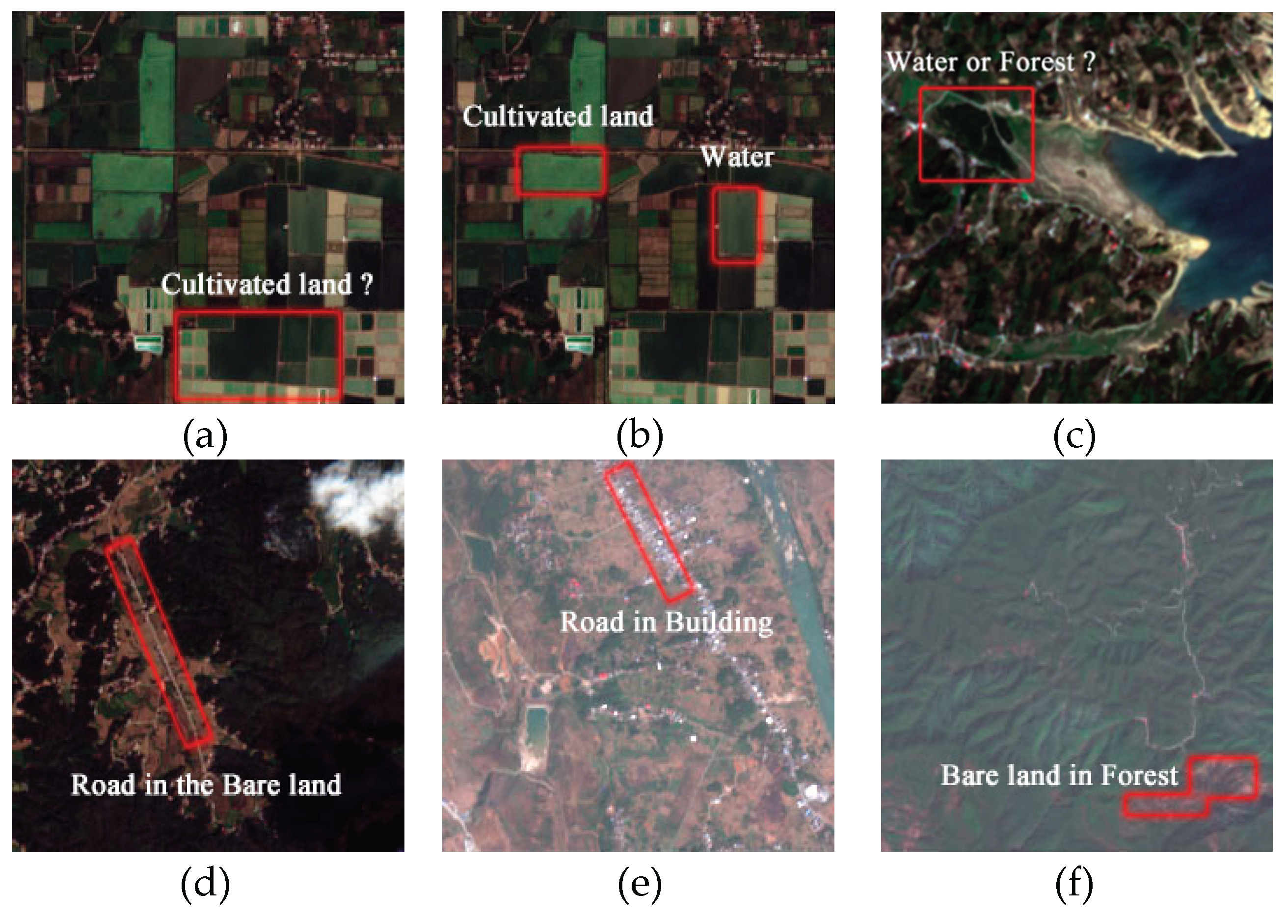
Figure 2.
Schematic architecture of the standard transformer block [17].
Figure 2.
Schematic architecture of the standard transformer block [17].
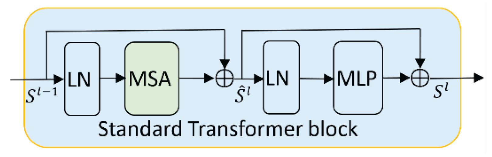
Figure 3.
Two consecutive Swin transformer blocks [20].
Figure 3.
Two consecutive Swin transformer blocks [20].
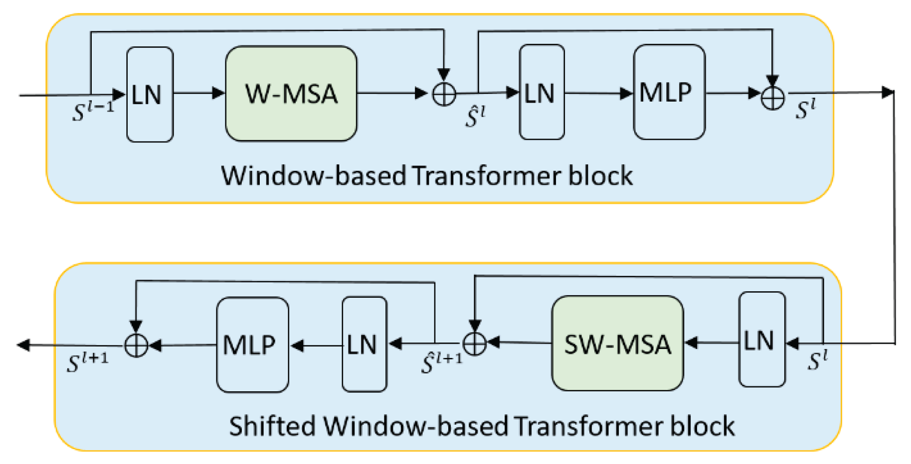
Figure 4.
Architecture of GSwin-Unet.
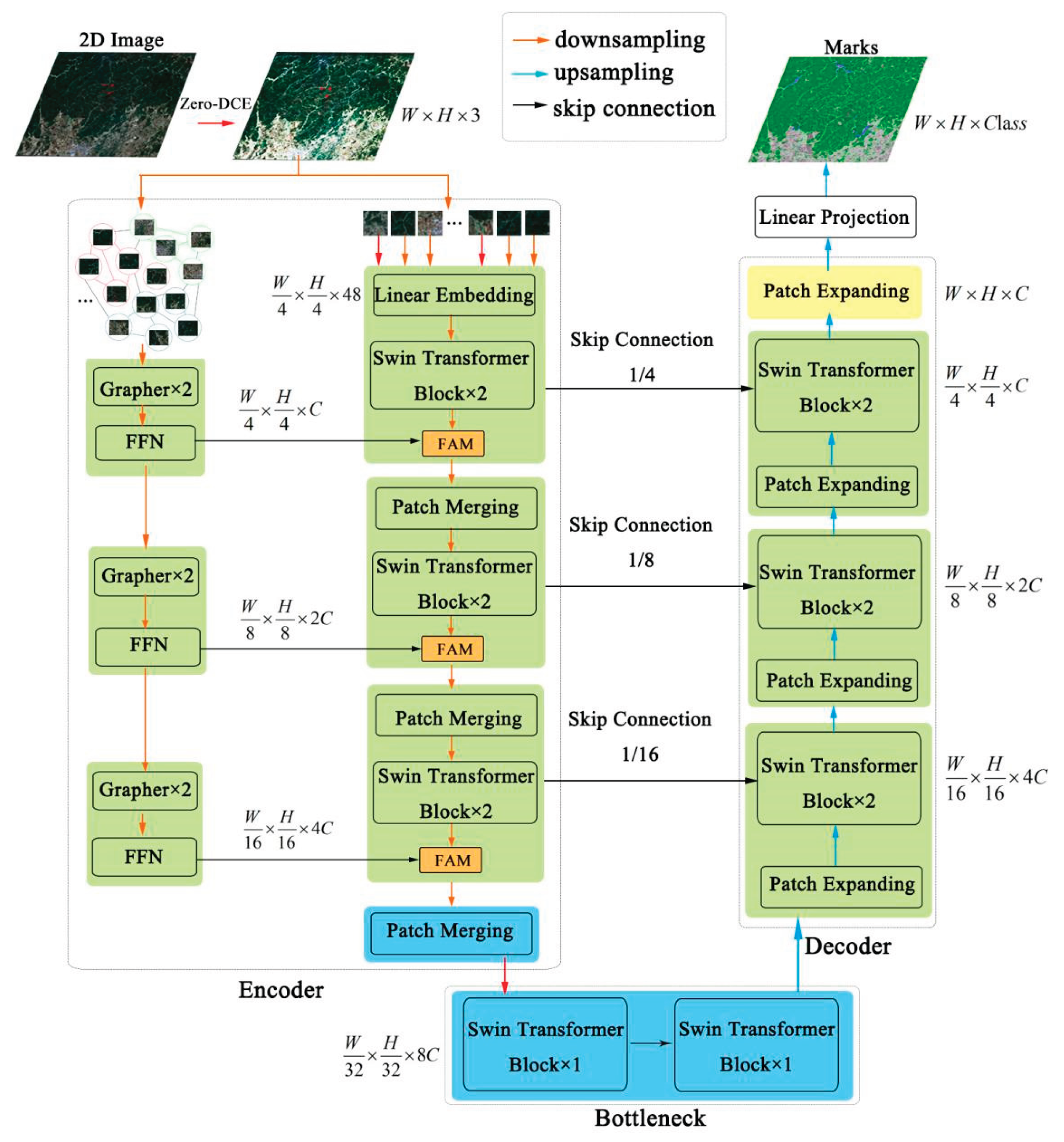
Figure 5.
VIG Block [23].
Figure 5.
VIG Block [23].
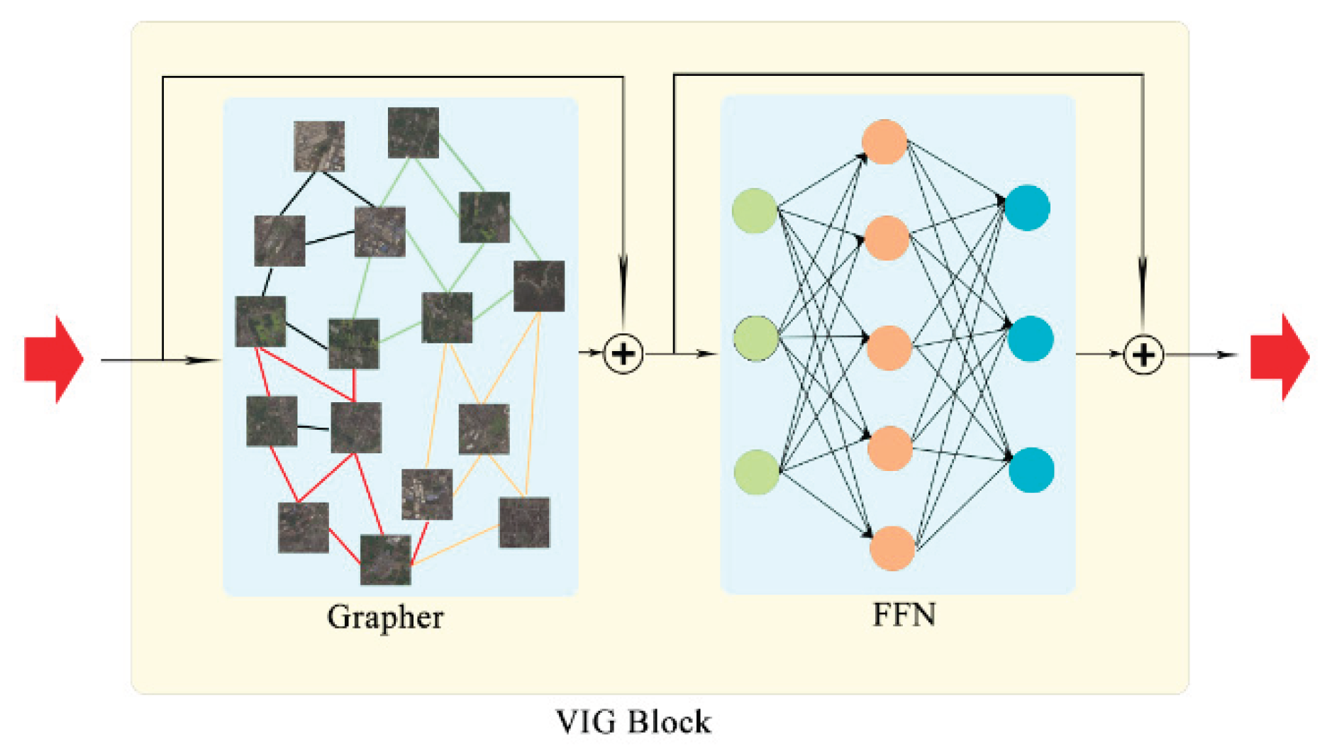
Figure 6.
The architecture of DCE-Net [72].
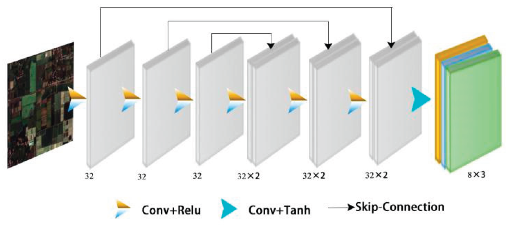
Figure 7.
Working mechanism of feature aggregation module. stands for matrix multiplication and stands for element-level addition.
Figure 7.
Working mechanism of feature aggregation module. stands for matrix multiplication and stands for element-level addition.
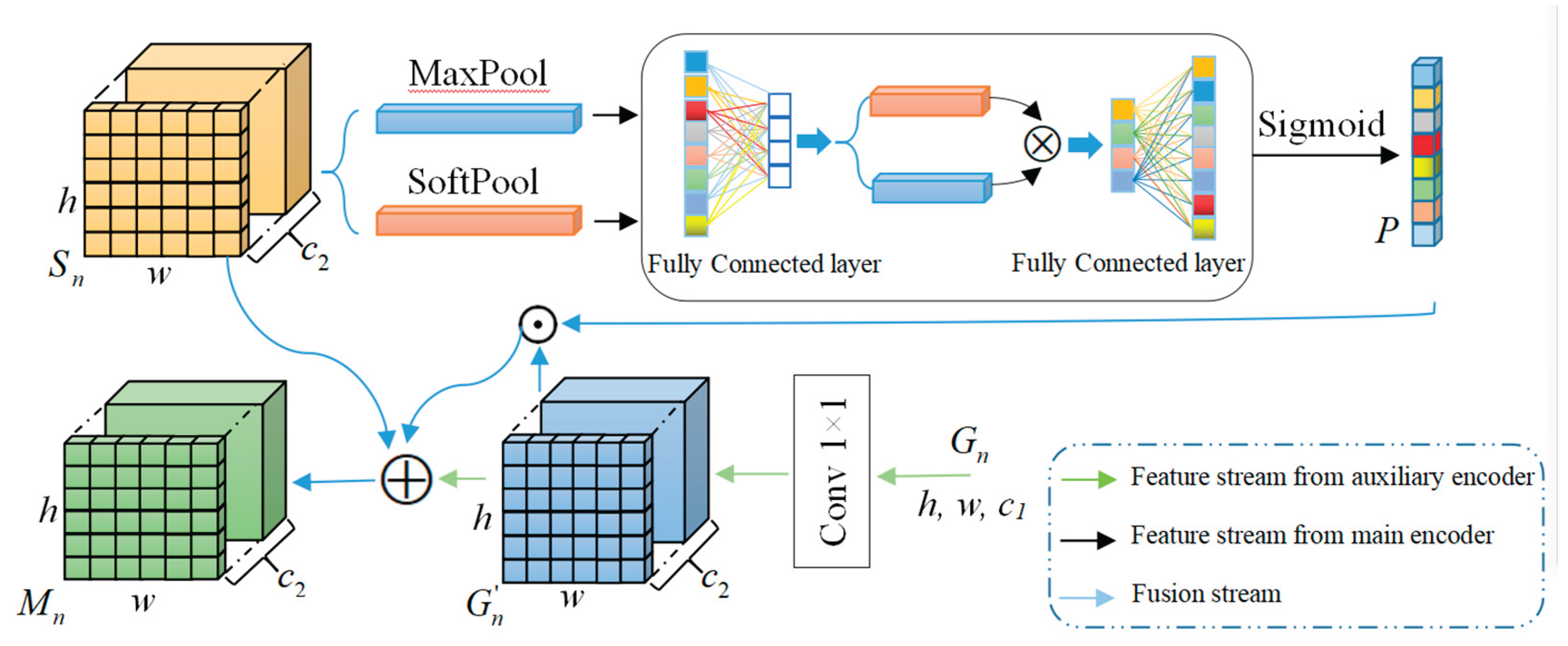
Figure 8.
Segmentation performance comparison: (a) GSwinU. (b) GswinU+FAM.
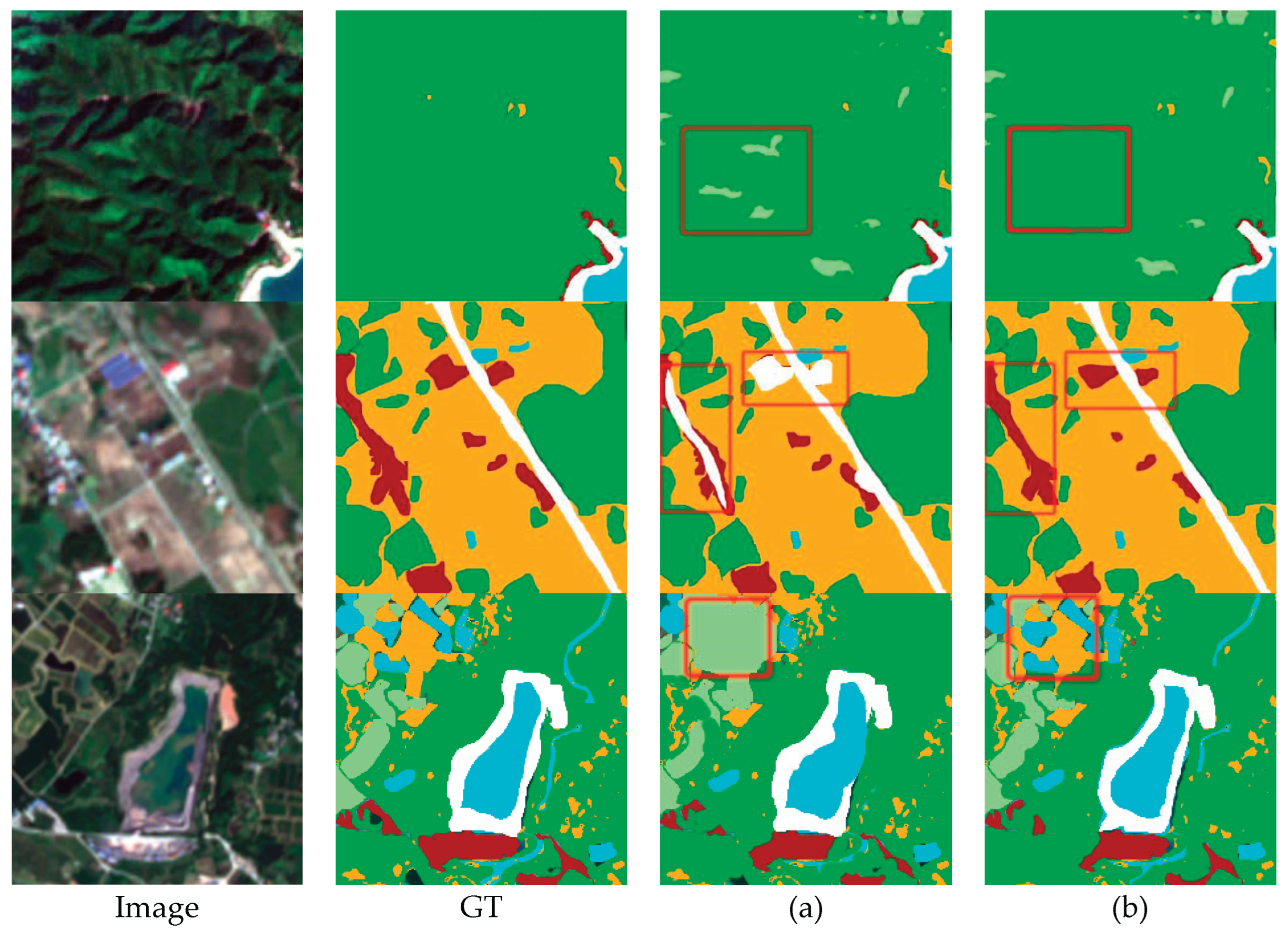
Figure 9.
Zero-Dice (ZD) Module Efficacy: (a) GSwinU+FAM. (b) GswinU+FAM+ZD.
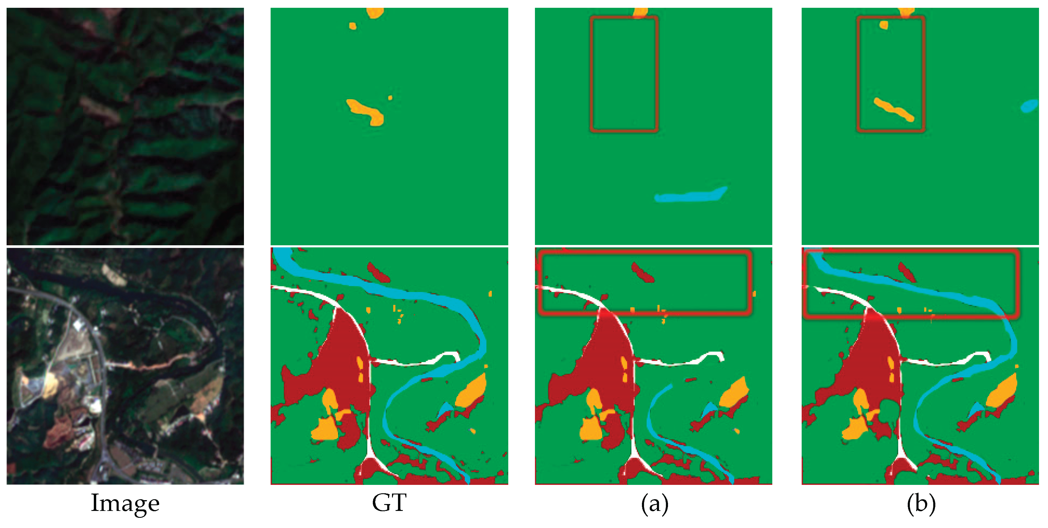
Figure 10.
Segmentation performance comparison across Loss-Functions.
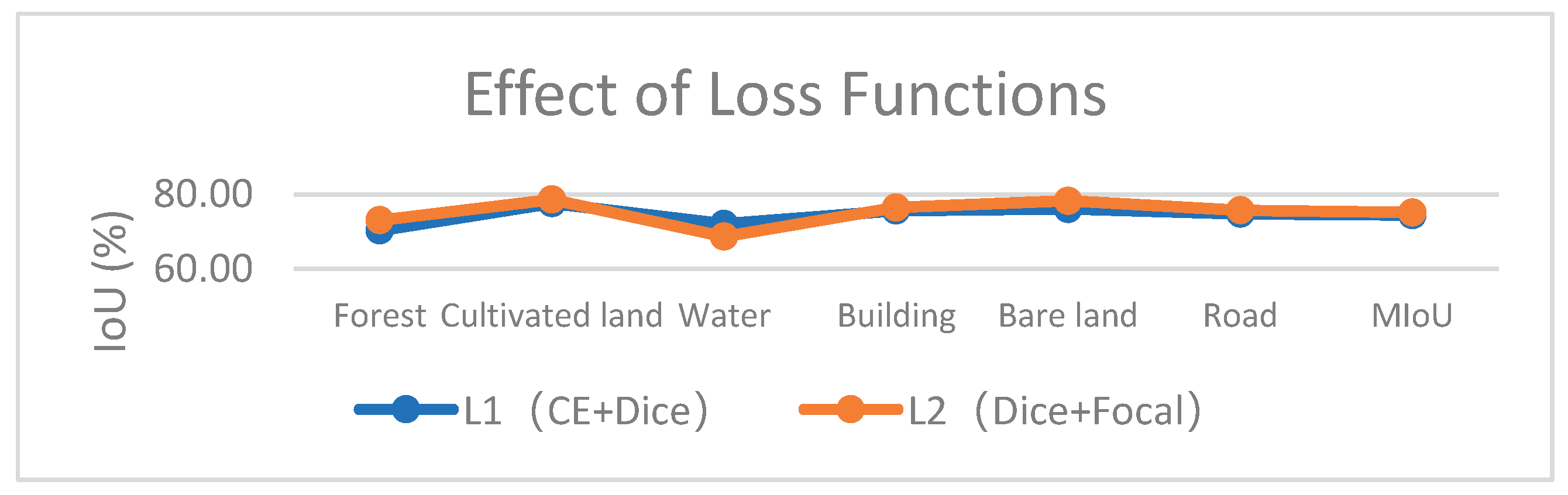
Figure 11.
Semantic segmentation instances on the RGB Forest dataset. (a) Deeplab V3+. (b) UNet. (c) Swin-UNet. (d) TransUnet. (d) GSwin-Unet.
Figure 11.
Semantic segmentation instances on the RGB Forest dataset. (a) Deeplab V3+. (b) UNet. (c) Swin-UNet. (d) TransUnet. (d) GSwin-Unet.
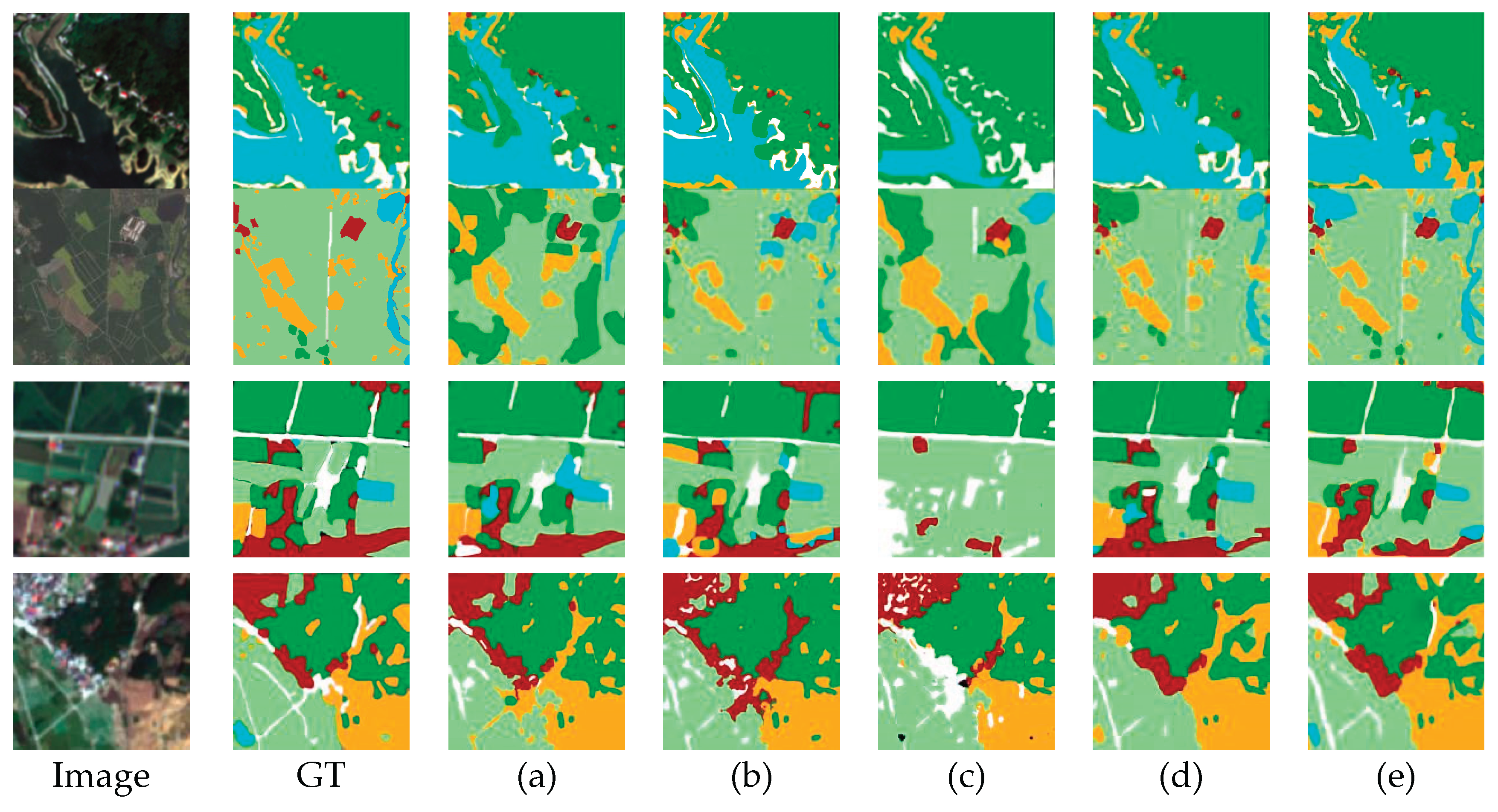
Figure 11.
Examples of semantic segmentation results on the NIRRG Forest dataset. (a) Deeplab V3+. (b) UNet. (c) Swin-UNet. (d) TransUnet. (d) GSwin-Unet.
Figure 11.
Examples of semantic segmentation results on the NIRRG Forest dataset. (a) Deeplab V3+. (b) UNet. (c) Swin-UNet. (d) TransUnet. (d) GSwin-Unet.
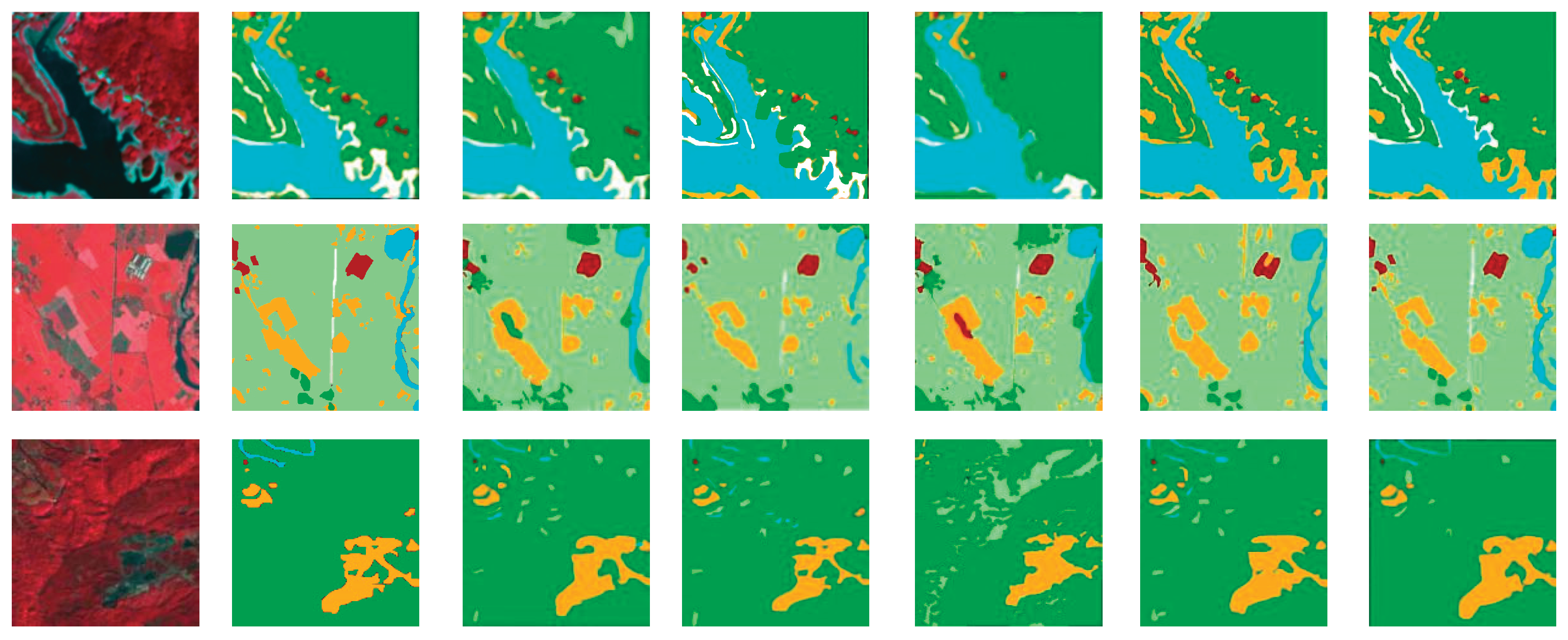
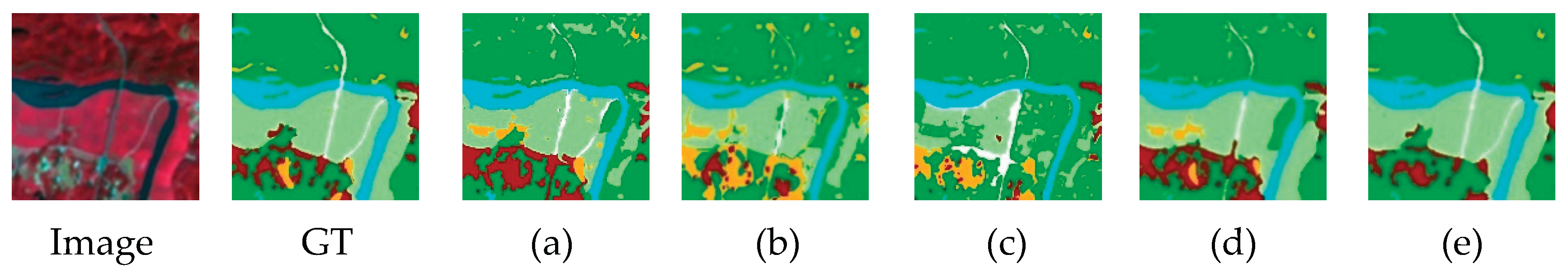

Table 1.
Network structure parameter settings.
| Stage | PyramidViG-Ti | Output size | Swin-transformer | Output size |
|---|---|---|---|---|
| Patch Partition | ||||
| Stem | Linear Embedding | |||
| Stage 1 | * | Swin-transformer Block×2 | ||
| Down sample | Patch Merging | |||
| Stage 2 | Swin-transformer Block×2 | |||
| Down sample | Patch Merging | |||
| Stage 3 | Swin-transformer Block×2 |
* D: Feature dimension (size); E: Ratio of hidden dimensions in FFN; K: Neighbors in GCN (Receptive field); H×W: Input image size.
Table 2.
Ablation Experiment of the Proposed Modules using the RGB Forest Dataset.
| Model Name | IoU (%) | Evaluation index | ||||||
| Forest | agricultural land | Water | Building | Bare land | Road | MIoU (%) | Ave.F1 (%) | |
| Swin-Unet | 67.23 | 70.63 | 67.26 | 66.67 | 62.83 | 62.50 | 66.19 | 79.62 |
| Swin-Unet+GCN+L1 | 67.23 | 76.03 | 66.95 | 74.14 | 75.65 | 70.00 | 71.67 | 80.43 |
| Swin-Unet+GCN+FAM+L1 | 70.09 | 76.27 | 72.07 | 75.63 | 74.79 | 74.53 | 73.90 | 84.80 |
| Swin-Unet+GCN+FAM+ZD+L1 | 70.34 | 77.59 | 72.07 | 75.63 | 76.07 | 74.77 | 74.41 | 85.30 |
| Swin-Unet+GCN+FAM+ZD+L2 | 73.04 | 78.63 | 68.64 | 76.47 | 78.26 | 75.70 | 75.13 | 85.96 |
Table 3.
Segmentation Results on the RGB Forest Dataset.
| Model Name | IoU (%) | Evaluation index | ||||||
| Forest | agricultural land | Water | Building | Bare land | Road | MioU (%) | Ave.F1(%) | |
| DeepLab V3+ | 57.60 | 68.66 | 61.67 | 78.38 | 78.07 | 63.96 | 68.06 | 80.73 |
| Unet | 61.67 | 73.17 | 70.54 | 79.46 | 73.17 | 62.07 | 70.01 | 82.20 |
| Swin-Unet | 67.23 | 70.63 | 67.26 | 66.67 | 62.83 | 62.50 | 66.19 | 79.62 |
| TransUnet | 66.39 | 75.21 | 68.10 | 76.52 | 79.65 | 68.75 | 72.44 | 80.23 |
| Gswin-Unet | 73.04 | 78.63 | 68.64 | 76.47 | 78.26 | 75.70 | 75.13 | 83.92 |
| MioU (%) | 65.19 | 73.26 | 67.24 | 75.5 | 74.40 | 66.60 | ||
Table 4.
Segmentation Results on the NIRRG Forest Dataset.
| Model Name | IoU (%) | Evaluation index | ||||||
|---|---|---|---|---|---|---|---|---|
| Forest | Agricultural land | Water | Building | Bare land | Road | MIoU (%) | Ave.F1 (%) | |
| DeepLab V3+ | 63.39 | 73.21 | 70.23 | 61.90 | 63.33 | 70.94 | 67.17 | 80.28 |
| Unet | 60.87 | 76.58 | 72.22 | 65.04 | 71.68 | 70.83 | 69.54 | 81.92 |
| Swin-Unet | 66.12 | 67.21 | 71.20 | 66.12 | 64.96 | 61.21 | 66.13 | 79.58 |
| TransUnet | 66.96 | 67.20 | 77.78 | 71.93 | 70.69 | 68.33 | 70.48 | 82.63 |
| GSwin-Unet | 69.72 | 69.67 | 76.67 | 74.14 | 76.36 | 70.94 | 72.92 | 84.30 |
| MIoU (%) | 65.41 | 70.77 | 73.62 | 67.83 | 69.40 | 68.45 | ||
Table 5.
Model Speed, Accuracy, and Parameters.
| Method | Parameters | RGB Forest | NIRRG Forest | ||
|---|---|---|---|---|---|
| Speed (FPS) | MIoU (%) | Speed (FPS) | MIoU (%) | ||
| UNet | 25.13 MB | 239 | 70.01 | 232 | 69.54 |
| Deeplab V3+ | 38.48MB | 76 | 68.06 | 74 | 67.17 |
| Swin-Unet | 25.89MB | 63 | 66.19 | 60 | 66.13 |
| TransUnet | 100.44 | 39 | 72.44 | 37 | 70.48 |
| GSwin-Unet | 160.97 | 9 | 75.13 | 8 | 72.92 |
Table 6.
Comparison Segmentation Result on the GID Dataset.
| Model Name | IoU (%) | Evaluation index | ||||||
|---|---|---|---|---|---|---|---|---|
| Forest | Farmland | Water | Building | Grass | Others | MIoU (%) | Ave.F1 (%) | |
| DeepLab V3+ | 57.48 | 70.00 | 64.71 | 78.57 | 76.32 | 63.96 | 67.17 | 80.28 |
| Unet | 61.67 | 72.13 | 67.83 | 79.46 | 73.17 | 62.93 | 69.54 | 81.92 |
| Swin-unet | 65.57 | 69.60 | 66.09 | 65.32 | 60.68 | 59.06 | 66.13 | 79.58 |
| TransUnet | 65.83 | 69.92 | 66.95 | 75.86 | 75.65 | 68.75 | 70.48 | 82.63 |
| GSwin-Unet | 71.30 | 74.79 | 71.43 | 73.33 | 73.55 | 72.90 | 72.92 | 84.30 |
Disclaimer/Publisher’s Note: The statements, opinions and data contained in all publications are solely those of the individual author(s) and contributor(s) and not of MDPI and/or the editor(s). MDPI and/or the editor(s) disclaim responsibility for any injury to people or property resulting from any ideas, methods, instructions or products referred to in the content. |
© 2025 by the authors. Licensee MDPI, Basel, Switzerland. This article is an open access article distributed under the terms and conditions of the Creative Commons Attribution (CC BY) license (http://creativecommons.org/licenses/by/4.0/).
Copyright: This open access article is published under a Creative Commons CC BY 4.0 license, which permit the free download, distribution, and reuse, provided that the author and preprint are cited in any reuse.


