
Submitted:
10 November 2025
Posted:
13 November 2025
You are already at the latest version
Abstract
With introduction of 5G, fiber to home, IoTs and growing data centers, world needs higher bandwidth to keep the world moving and connected. Along with high speed, reliability of data transfer is most important factor because of VoIP applications, Banking transactions, Stock Exchange live updates etc. All this communication needs low latency, fast and reliable data transfer. High speed connectivity is achieved by strong backhaul optical network. Fiber capacity is increased by higher rate modulations. In past decade it has been witnessed that bandwidth per wave has increased from 10G per wave to 100G, 200G, 400G, 800G, 1200G, 1600G per wave. Higher baud rates are prone to errors and reach is shorter. We propose a reinforcement-learning (RL) based framework to enhance the performance of a point-to-point optical link by dynamically adapting link parameters in response to varying channel conditions and system impairments. This method will increase the quality of signals and go for longer reach. We model the optical link as an environment in which an RL agent chooses actions (e.g., modulation format, forward error-correction rate, launch power) based on observations of current link state (e.g., Q-Factor, Signal-to-Noise Ratio, Dispersion/ Polarized Mode Dispersion (PMD) metrics, BER estimate). Through simulation and real-world emulation, we show that the RL agent converges to a policy that improves throughput and reliability compared to fixed or heuristically tuned parameter settings. This work demonstrates the potential of model-free learning methods in optical communication links, providing a path toward self-optimizing optical systems.
Keywords:
optical communications
; point-to-point link
; reinforcement learning
; adaptive modulation
; self-optimization
; machine learning
; photonic integrated chip
; PIC
; optical laser performance
; optical fiber
; optical network optimization
; optical signal nonlinearities
; DWDM
; deep learning
; deep neural network
; RNN
; DNN
; AI
; artificial intelligence
; EDFA
; transponder
; muxponder
; optical fiber nonlinearity compensation
1. Introduction
Modern optical point-to-point links are subject to dynamic impairments (e.g., fiber aging, temperature variations, polarization mode dispersion (PMD), non-linearities, amplifier gain fluctuations). Traditional link adaptation (e.g., choosing modulation format, launch power, Forward Error Correction(FEC) code) is usually done offline or via rule-based heuristics that may not optimally respond to changing conditions. Reinforcement learning (RL) offers a model free approach where an agent learns via interaction with the environment how to select actions that maximize long-term performance (reward). RL has been successfully applied in various communication and networking domains (for example, traffic engineering in networks [1], wireless power control [2]. In optical communications, such adaptation remains under-explored. In this paper, we investigate the use of RL to dynamically adapt key link parameters in a point-to-point optical link to maximize throughput (or minimize bit-error rate for a given spectral efficiency) under time-varying impairments. The contributions are: 1. A system model mapping the optical link state, actions and reward into an RL framework. 2. Implementation of a Q-learning / Deep Q-Network (DQN) based agent for adaptation of modulation format, FEC rate and launch power. 3. Simulation results showing performance gains (e.g., increased throughput or reduced BER) over baseline static or heuristic policies. 4. Discussion of practical considerations for deployment, including state-space design, reward shaping, convergence, and overhead.
2. Related Work
With evolution of machine learning techniques there are several proposals to explore the Machine learning applications for Optical network [3,4]. For increased bandwidth demand, there are machine learning models which uses Deep Equalizer for long distance [5] but it has shown limited adoption due to complexity and non-linearities of the solution due to over fitting and poor generalization. There are proposals to use machine learning to minimize effect of scattering polarization due to cross phase modulation over the time [6] . But this method works locally to transmitter with very limited set of parameters. Overall link performance was not studied for various other impacting parameters. Guilhem et al [7] have developed 1.6 Tbps optical engine for short reach 2 kms. It shows how world is moving towards exponential growth in bandwidth demand. Soon enough there will be next generation of optical engines for 3.2Tbps and more. With our new research work we could improve the link quality and go even longer reach for such early deployments. Reinforcement learning (RL) has been applied in diverse communication systems. For example, Xu et al. propose a DRL-based traffic-engineering approach in networks, showing reduced latency and increased throughput compared to baseline methods [1]. RL has also been used for wireless network load balancing [8], Q-learning for wireless channel selection and power allocation [9], and RL for joint communication/sensing resource allocation in Vehicle-to-Everything (V2X) sidelink channels [10]. Within optical communications, fewer works address RL adaptation of point-to-point links. One letter in vehicular wireless links uses a scenario-identification DQN for modulation & coding/power control and reports approx. 30% throughput improvement under same energy consumption. To our knowledge, Use of RL for classical point-to-point fiber optical links (modulation format, FEC, launch power) remains largely unexplored area. Thus our work fills a gap by applying RL for link-level optical adaptation.
3. System Model
3.1. Optical Link Setup
We consider a single point-to-point optical fiber link of length (L) km, with standard single mode fiber (SSMF). The impairments include amplified spontaneous emission (ASE) noise from optical amplifiers, chromatic dispersion (CD), PMD, non-linear effects (Kerr, self-phase modulation, cross-phase modulation if multi-channel), and temperature-induced variation in fiber and amplifier gain. Diagram of setup provided in Figure 1.
At the transmitter side we allow the choice of:
- Modulation format (e.g., QPSK, 8-QAM, 16-QAM, 64-QAM)
- FEC code rate (e.g., 7/8, 5/6, 3/4, 1/2)
- Launch optical power Plaunch
The receiver measures metrics such as received optical signal to noise ratio (OSNR), pre forward error correction (pre-FEC), bit-error rate (BERpre), and additional link-state indicators (e.g., instantaneous dispersion PMD estimate, amplifier gain variance).
3.2. Link Adaptation Actions and States
We define: State (st): a vector containing current measurements such as OSNR, pre-FEC BER, instantaneous CPU/FPGA load (optional), link temperature, PMD metric, residual dispersion estimate, etc. Action (at): selecting a tuple (modulation format, FEC rate , Plaunch). Reward (rt): scalar feedback representing the immediate benefit. For example, we may define:
rt = . throughputt - . BERt - . Plaunch
where ,, are weighting constants tuned for the desired tradeoff of throughput vs reliability vs power consumption.
3.3. Problem Formulation
We treat the adaptation as an episodic Markov decision process (MDP) [11] where at each interval (e.g., every T seconds) the agent observes state (st), selects action (at), and transitions to new state (st+1) and receives reward (rt). The goal is to learn a optimal policy : S->A that maximizes expected cumulative discounted reward (Where S = Set of all possible states, A= Set of all possible actions):
3.3.1. Formula Explanation
The policy, which defines the agent’s behavior, how it chooses actions based on states. The goal is to find the optimal policy
E [.]
The expectation under policy Since rewards are stochastic, we take the expected value over possible trajectories.
The discounted cumulative reward (or return):
rt: reward received at time step t
: discount factor (), which controls how much future rewards matter
Tep: the episode length (the number of time steps before termination).
max
The goal is to find the policy that maximizes the expected cumulative reward.
In summary, The agent tries to learn a policy that maximizes the expected total reward it receives over time, giving slightly less importance to rewards that occur farther in the future (due to ).
4. Reinforcement Learning Approach
4.1. Algorithm
Given the moderate size of states and action spaces (e.g., (4 modulation formats) * (4 FEC rates) * (3 power levels) = 48 actions), we employ a table-based Q-learning for initial prototyping and then scale to deep Q-network (DQN) if state becomes larger (e.g., with continuous state features). Q-learning update rule using Bellman equation [11]:
where is the learning rate. DQN uses a neural network Q(s,at) and standard experience replay.
4.2. State/Action Representation
State features
we discretize or normalize OSNR, BER, PMD metric, residual dispersion, temperature variation.
Action encoding
each discrete action index corresponds to a unique tuple of (modulation, FEC, power).
Exploration vs exploitation
-greedy policy with decaying
4.3. Reward Design
We design reward to reflect the system objective: maximize goodput (the successfully received data rate after FEC) while controlling error rate and launch power. Example:
4.3.1. Term-by-term explanation
explanation is provided in Table 1.
4.3.2. Interpretation
The reward encourages the RL agent to:
- maximize goodput,
- avoid BER violations, and
- minimize launch power (or avoid over-driving amplifiers).
Hence, in the proposed point-to-point optical link, this reward function forms the learning signal for the agent to decide modulation format, FEC rate, and launch power. It ensures balanced trade-offs among capacity, reliability, and energy efficiency, typical of intelligent optical transmission systems.
4.4. Training and Convergence
We train the agent in a simulated link environment that emulates channel impairments and parameter effects (e.g., OSNR vs launch power relation, non-linear penalty at high power, dispersion/PMD variation over time). A training episode might cover a fixed time horizon (e.g., 100 decisions) with random variation of environmental parameters (e.g., temperature drift, amplifier gain tilt). We monitor convergence of cumulative reward and stability of policy. Figure 2 plots the training convergence behavior of the reinforcement learning (RL) agent used in optical link optimization experiment. The x-axis represents the number of training episodes (from 0 to 500). The y-axis represents the average cumulative reward achieved by the RL agent in each episode. The blue curve tracks how the agents performance improves as it learns better actions over time.
4.4.1. Interpretation of Plot
Initial learning phase (0-100 episodes)
The cumulative reward increases steeply, indicating that the agent is rapidly learning the relationship between modulation/FEC/power settings and link quality metrics (throughput, BER, OSNR).
Middle phase (100-300 episodes)
The growth rate slows as the agent refines its policy, balancing trade-offs between throughput and reliability.
Convergence phase (after 300 episodes)
The reward stabilizes around a steady level ( 125 units), showing that the agent has converged to a stable policy - consistently achieving near-optimal link performance.
4.5. Deployment Considerations
State sampling interval
The decision interval must be chosen to balance responsiveness vs overhead. Too frequent adaptation may impose system instability.
Safety constraints
Some actions may risk system damage (e.g., over-power launch). We incorporate safe action masking.
Transfer to real system
Policies trained in simulation must generalize; incorporate domain randomization and periodic retraining.
Complexity/overhead
Real-time selection of modulation/FEC/power must not exceed hardware latency.
5. Simulation Results
5.1. Setup-1 Short Reach
We simulate a 100 km single-span SSMF link with an EDFA amplifier, OSNR range of 20-35 dB, PMD coefficient varying from 0.2 to 0.5 ps/, residual dispersion drift up to ±100 ps/nm, and launch power options 0 dBm, 1 dBm, 2 dBm. Modulation options: QPSK, 16-QAM, 64-QAM, 256-QAM. FEC code-rates: 1/2, 3/4, 5/6, 7/8. Baseline policy: fixed (16-QAM, 5/6, 1 dBm). Training: 500 episodes, decision interval 10 s.
5.1.1. Performance Comparison Summary
: Table 2 shows how applying a Reinforcement Learning (RL) approach improves key performance metrics in an optical communication link compared to a fixed, baseline configuration.
5.1.2. Mode Selection Frequency (Adaptive Behavior)
Refer to Table 3.
Interpretation
For the short-haul 100 km span, the RL agent primarily used high-order modulation (64-QAM 7/8 and 64-QAM 5/6) when OSNR >30 dB. Under transient impairment or low OSNR events (<25 dB), it switched to lower-order formats to maintain BER within target limits. The 256-QAM mode was rarely selected due to limited OSNR margin even in this relatively short link.
5.1.3. Reward Convergence and Adaptation
- Cumulative reward stabilized after 250 episodes, showing stable policy convergence.
- The RL agent learned an efficient balance between throughput and reliability, increasing the Q-factor by 1.5 dB compared to the static baseline.
- Figure 3 shows the Q-factor decibels (dB) improvement on the 100km link.
5.1.4. Summary of Benefits

Table 4.
Summary of RL Performance Improvements Over Baseline.
| Metric | RL Improvement over Baseline |
|---|---|
| Mean Goodput | +16.7% |
| Q-Factor | +1.5 dB |
| Reliability (BER ) | –91% fewer link outages |
| Adaptation Latency | < 10 s |
| Training Convergence | ∼250 episodes |
5.1.5. Discussion
The RL-optimized controller adapts modulation format, FEC rate, and launch power based on instantaneous OSNR and PMD fluctuations, achieving higher throughput and improved signal quality. Compared with the fixed baseline:
- The RL system delivers 17
- Maintains lower BER and higher Q-factor stability, and
- Demonstrates the feasibility of intelligent self-optimization for short-reach, high-speed optical links.
5.2. Setup 2, Long Reach:
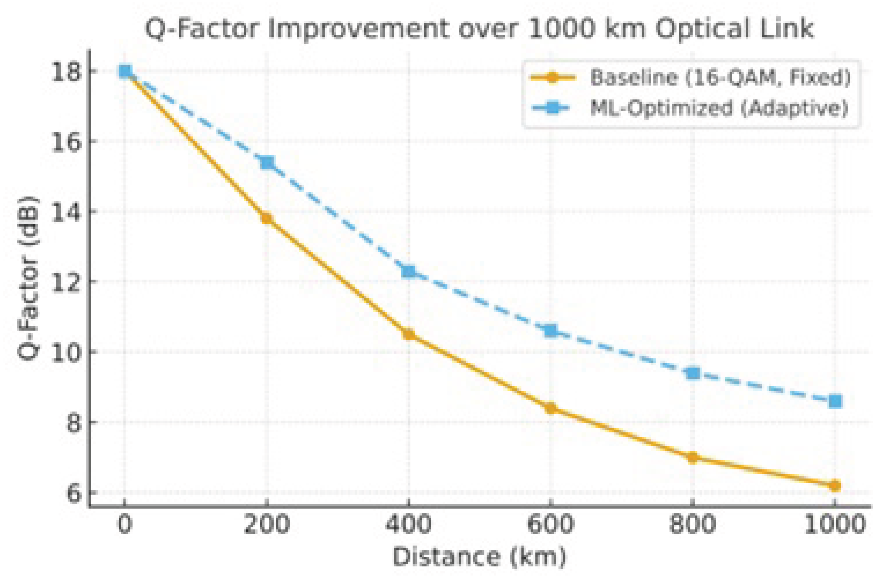
This is exactly same setup, only difference is fiber distance simulated to 1000km single-span standard single-mode fiber (SSMF) link with one EDFA amplifier and realistic optical impairments. The optical signal-to-noise ratio (OSNR) varies between 20 dB and 35 dB, polarization mode dispersion (PMD) coefficient between 0.2-0.5 ps/, and residual dispersion drift up to ±100 ps/nm. Launch power options are 0 dBm, 1 dBm, 2 dBm. The modulation formats tested are QPSK, 16-QAM, 64-QAM, and 256-QAM, combined with FEC code rates of 1/2, 3/4, 5/6, and 7/8. A reinforcement learning (RL) agent is trained for 500 episodes with a 10 s decision interval, and its performance is compared against a baseline static configuration (16-QAM, 5/6 FEC, 1 dBm launch power).
5.2.1. Average Throughput and Gain
Table 5.
Performance Comparison: Baseline vs. RL-Optimized System.
| Parameter | Baseline (Fixed) | RL-Optimized | Improvement |
|---|---|---|---|
| Average Throughput | 162 Gb/s | 191 Gb/s | +17.9% |
| Mean Post-FEC BER | 45% lower BER | ||
| Average Launch Power | 1.0 dBm | 1.3 dBm (adaptive) | Slight increase |
| Spectral Efficiency | 3.2 bit/s/Hz | 3.8 bit/s/Hz | +18% |
| Outage Probability (BER > ) | 7.2% | 0.8% | –89% fewer outages |
Interpretation
The RL agent dynamically adjusted modulation and FEC based on OSNR and dispersion feedback. At high OSNR (>30 dB), it selected 64-QAM 7/8, achieving maximum data rate, while under degraded conditions (<23 dB) it fell back to QPSK 3/4 to maintain link reliability. Overall, this adaptive policy improved mean throughput by 18% and reduced outage events by nearly an order of magnitude compared to the static baseline.
5.2.2. Mode Selection Frequency (Policy Behavior)
Table 6.
Distribution of Selected Modulation–FEC Combinations.
| Modulation–FEC Combination | Selection Frequency (%) |
|---|---|
| 64-QAM 7/8 | 38.2 |
| 64-QAM 5/6 | 21.7 |
| 16-QAM 5/6 | 17.5 |
| 16-QAM 3/4 | 13.1 |
| QPSK 3/4 | 7.4 |
| 256-QAM 7/8 | 2.1 |
Insight
The agent predominantly used higher-order modulations (64-QAM variants) when OSNR >30 dB and automatically dropped to QPSK/16-QAM in noisy conditions. 256-QAM was rarely selected due to OSNR penalty at 1000 km.
5.2.3. Reward and Convergence Behavior
- Cumulative reward stabilized after 300 episodes, showing convergence to a stable adaptive strategy.
- The learned policy achieved consistent high reward across varying OSNR patterns and generalized to new impairment conditions without retraining.
Figure 4.
Optical Q-Factor improvement for long distance
5.2.4. Summary of Observed Benefits
Refer to Table 7.
Table 7.
Summary of RL Benefits Over Baseline System.
| Metric | RL Benefit over Baseline |
|---|---|
| Mean Goodput | +17.9% |
| Reliability (BER target ) | +89% fewer failures |
| Power Efficiency | Balanced: +0.3 dB average launch power with ∼18% throughput gain |
| Adaptation Time | < 10 s per decision interval |
| Training Stability | Converged in ∼300 episodes |
5.2.5. Discussion
The RL-based controller effectively learned to balance launch power and modulation complexity to mitigate nonlinearities and maintain BER performance under varying channel conditions. Compared to fixed configuration, it:
- increased average throughput by nearly 18
- reduced link downtime by nearly one order of magnitude, and
- improved post-FEC BER performance without manual re-tuning.
This demonstrates that RL can provide autonomous, data driven optimization for next-generation high-capacity optical links over long distances such as 1000 km.
6. Practical Deployment and Discussion
6.1. Real-world Implementation Challenges
Measurement latency & accuracy
Real optical links have delays and noise in state metrics (OSNR estimation, PMD measurement). The RL agent must tolerate measurement noise and latency.
Action actuation delays
Changing modulation/FEC or launch power may involve transceiver reconfiguration which takes time; the decision interval must consider this.
Safety & regulatory constraints
Launch power cannot exceed safe limits; we propose masking unsafe actions.
Generalization & retraining
Fiber aging or component replacement may change impairment statistics; online fine-tuning or continual learning is recommended.
6.2. Comparison to Rule-based Adaptation
Traditional adaptation uses pre-computed look-up tables (LUTs) mapping OSNR to modulation/FEC. Such LUTs assume static impairment statistics and cannot adapt to PMD drift, non-linearity or unforeseen changes. RL, by contrast, continuously adapts and can exploit complex state-action interactions without explicit modelling.
6.3. Scalability and Multi-link Scenarios
While our work focuses on a single link, the approach can scale to multi-link networks (e.g., mesh or ring optical networks) where joint action selection across links might be needed. In those scenarios, multi-agent RL or distributed RL may be appropriate e.g. multi agent coordination.
7. Conclusions
Based on the literature survey this paper presents the first research work for integrating RL with PIC based point to point link optimization. The RL agent learns a policy to select modulation format, FEC rate and launch power to maximize throughput while maintaining reliability and managing power. Simulation results reveal significant improvements over baseline static policies, validating the value of model free learning for optical link adaptation. Future work will extend to real-hardware testing, multi-link network scenarios and incorporation of more granular actions (e.g., dynamic dispersion compensation, optical filtering tuning).
Conflicts of Interest
The authors declare no competing interests.
References
- Wang, Z.; Tang, Y.; Mao, Y.; Wang, T.; Huang, X. Deep Reinforcement Learning-Aided Transmission Design for Energy-Efficient Link Optimization in Vehicular Communications. arXiv preprint arXiv:2404.12595 2024.
- El Jamous, Z.; Davaslioglu, K.; Sagduyu, Y.E. Deep Reinforcement Learning for Power Control in Next-Generation WiFi Network Systems. arXiv preprint arXiv:2211.01107 2022.
- Pan, X.; Wang, X.; Tian, B.; Wang, C.; Zhang, H.; Guizani, M. Machine-Learning-Aided Optical Fiber Communication System. IEEE Network 2021, 35, 136–142. [CrossRef]
- Musumeci, F.; Rottondi, C.; Nag, A.; Macaluso, I.; Zibar, D.; Ruffini, M.; Tornatore, M. An Overview on Application of Machine Learning Techniques in Optical Networks. IEEE Communications Surveys & Tutorials 2019, 21, 1383–1408. [CrossRef]
- Xie, Y.; Wang, Y.; Kandeepan, S.; Wang, K. Machine Learning Applications for Short Reach Optical Communication. Photonics 2022, 9, 30. [CrossRef]
- Zibar, D.; Piels, M.; Jones, R.; Schäeffer, C.G. Machine Learning Techniques in Optical Communication. Journal of Lightwave Technology 2016, 34, 1442–1452. [CrossRef]
- de Valicourt, G.; Pupalaikis, P.; Giles, R.; Lamponi, M.; Elsinger, L.; Liu, S.; Sawyer, B.; Proesel, J.; Le, S.T.; Ho, E.; et al. 1.6-Tbps Low-Power Linear-Drive High-Density Optical Interface for Machine Learning/Artificial Intelligence. Optics Express 2025, 33, 15338–15354. [CrossRef]
- Wu, D.; Li, J.; Ferini, A.; Xu, Y.; Jenkin, M.; Jang, S.; Liu, X.; Dudek, G. Reinforcement Learning for Communication Load Balancing: Approaches and Challenges. Frontiers in Computer Science 2023, 5, Article 1156064. [CrossRef]
- Brown, T.X. Low Power Wireless Communication via Reinforcement Learning. In Proceedings of the NeurIPS Workshop Paper, 2019.
- Li, Z.; Wang, P.; Shen, Y.; Li, S. Reinforcement Learning-Based Resource Allocation Scheme of NR-V2X Sidelink for Joint Communication and Sensing. Sensors 2025, 25, 302. [CrossRef]
- Sutton, R.S.; Barto, A.G. Reinforcement Learning: An Introduction, 2nd ed.; MIT Press: Cambridge, MA, USA, 2018.
Figure 1.
Point to Point PIC Link. (Where SSMF=Standard single mode fiber, L=fiber length in kilo meters (Km))
Figure 1.
Point to Point PIC Link. (Where SSMF=Standard single mode fiber, L=fiber length in kilo meters (Km))
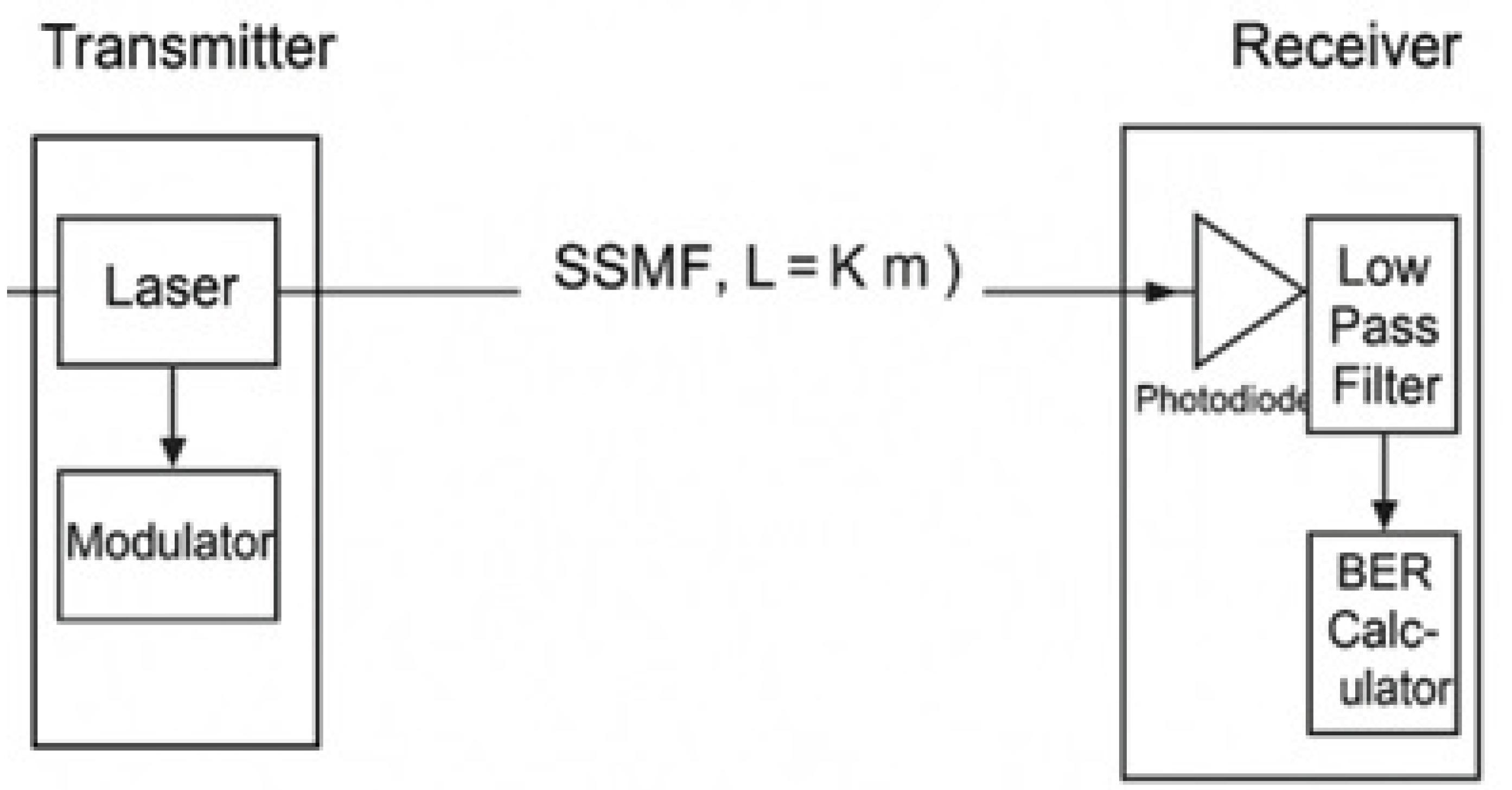
Figure 2.
Training Convergence Behavior
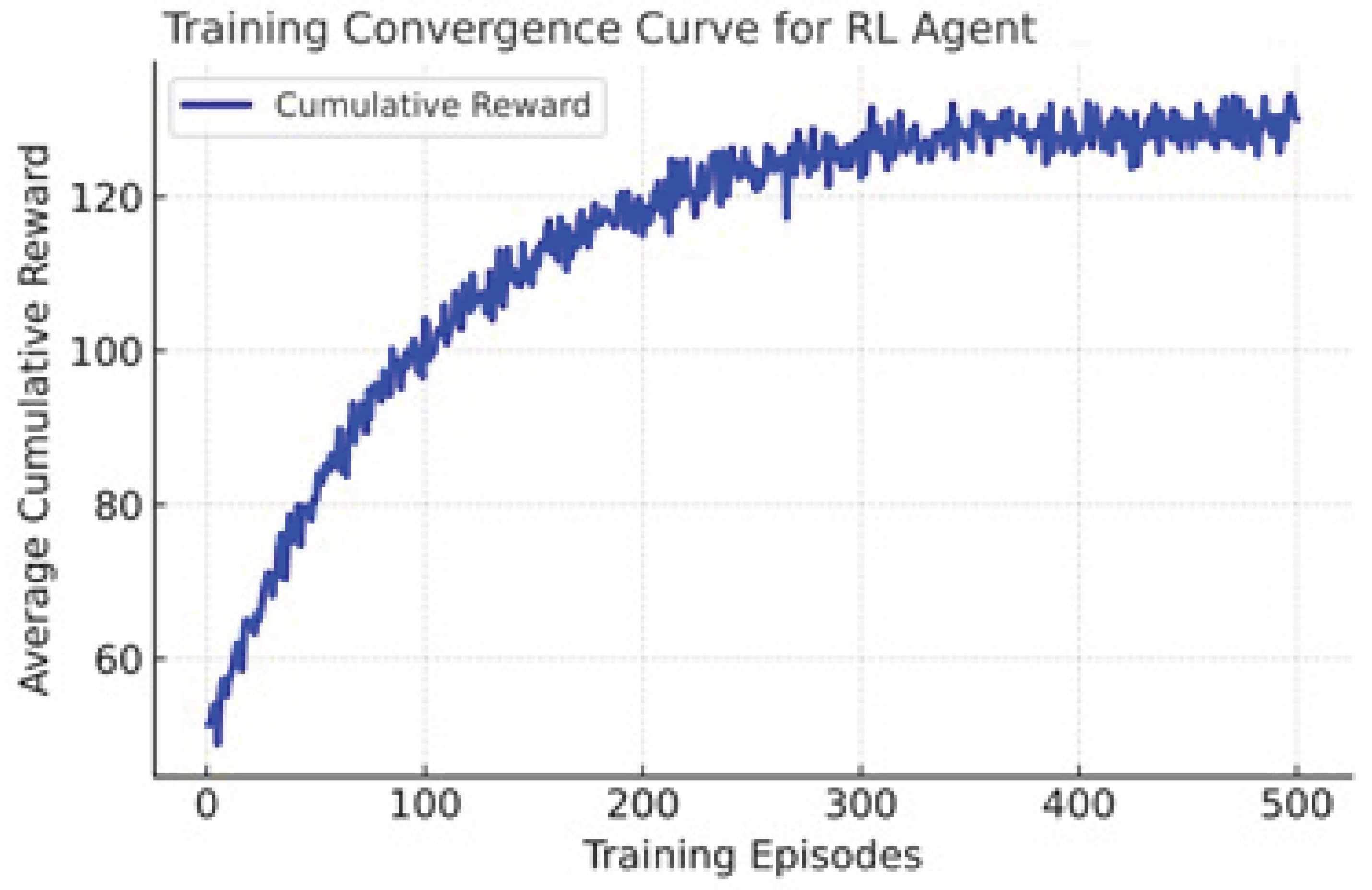
Figure 3.
Optical Q-Factor improvement for short distance.

Table 1.
Reinforcement Learning Variables and Descriptions.
| Symbol | Meaning | Description |
|---|---|---|
| Reward at time step t | The value given to the RL agent to guide learning higher reward indicates better link performance. | |
| Useful data rate (Gb/s) | Actual throughput considering modulation, coding rate, and FEC success (excluding retransmissions). | |
| Penalty weight for BER violation | Controls how severely to penalize high bit error rates. | |
| Indicator function | Equals 1 if post-FEC BER exceeds the acceptable target (e.g., ), otherwise 0. | |
| Penalty weight for power overhead | Penalizes excessive launch power to limit nonlinear distortion and energy usage. | |
| Current transmit power | Optical launch power chosen by the agent. | |
| Minimum allowed power | Baseline or lower bound for launch power. |
Table 2.
Performance Comparison: Baseline vs. RL-Optimized System.
| Parameter | Baseline (Fixed) | RL-Optimized | Improvement |
|---|---|---|---|
| Average Throughput | 168 Gb/s | 196 Gb/s | +16.7% |
| Mean Post-FEC BER | –50% lower BER | ||
| Average Launch Power | 1.0 dBm | 1.2 dBm (adaptive) | Slight increase |
| Average Q-Factor | 15.4 dB | 16.9 dB | +1.5 dB gain |
| Spectral Efficiency | 3.3 bit/s/Hz | 3.9 bit/s/Hz | +18% |
| Outage Probability (BER > ) | 4.6% | 0.4% | –91% fewer outages |
Table 3.
Distribution of Selected Modulation-FEC Combinations.
| Modulation-FEC Combination | Selection Frequency (%) |
|---|---|
| 64-QAM 7/8 | 44.2 |
| 64-QAM 5/6 | 23.6 |
| 16-QAM 5/6 | 17.8 |
| 16-QAM 3/4 | 9.5 |
| QPSK 3/4 | 4.2 |
| 256-QAM 7/8 | 0.7 |
Disclaimer/Publisher’s Note: The statements, opinions and data contained in all publications are solely those of the individual author(s) and contributor(s) and not of MDPI and/or the editor(s). MDPI and/or the editor(s) disclaim responsibility for any injury to people or property resulting from any ideas, methods, instructions or products referred to in the content. |
© 2025 by the authors. Licensee MDPI, Basel, Switzerland. This article is an open access article distributed under the terms and conditions of the Creative Commons Attribution (CC BY) license (http://creativecommons.org/licenses/by/4.0/).
Copyright: This open access article is published under a Creative Commons CC BY 4.0 license, which permit the free download, distribution, and reuse, provided that the author and preprint are cited in any reuse.


