
Submitted:
30 October 2025
Posted:
03 November 2025
You are already at the latest version
Abstract
Classical binomial interval methods often exhibit poor performance when applied to extreme conditions, such as rare-event scenarios or small-sample estimations. Recent frequentist and Bayesian approaches have improved coverage in small-samples and rare-events but typically rely on fixed error margins that do not scale with the magnitude of the proportion, thus distorting uncertainty quantification at the extremes. As an alternative method to reduce these boundary distortions, we propose a novel hybrid approach that blends Bayesian, frequentist, and approximation-based techniques to estimate robust and adaptive intervals. The variance incorporates sampling variability, Wilson score margin of error, a tuned credible level, and a gamma regularisation term that is inversely proportional to sample size. Extensive simulation studies and real-data applications demonstrate that the proposed method consistently achieves competitive or superior coverage proportions with narrower or more conservative interval widths compared to Jeffreys and Wilson score intervals, especially for rare and extreme events. Geometric analysis of the tuning curves reveals convex-to-linear transitions and mirrored symmetry across the rare-extreme spectrum, which underscores its boundary sensitivity and adaptivity. Our method offers a theoretically grounded, computationally efficient and practically robust estimation of rare-event intervals which has applications in safety-critical reliability, epidemiology, and early-phase clinical trials.
Keywords:
rare events
; adaptive variance
; bayesian interval
; credible-level tuning
1. Introduction
Rare event phenomena such as emerging disease outbreaks, earthquakes, and industrial defects are typically characterised by extremely low probability of occurrence. Estimation of binomial proportions for such events poses significant challenges, particularly due to the inadequacy of conventional confidence interval methods. Classical approaches, such as the Wald interval, frequently perform poorly for these events due to their reliance on asymptotic normality, which fails as the true proportion approaches the extreme boundaries of the binomial proportions (Wilson, 1927; Agresti and Coull, 1998). The Clopper-Pearson interval also tends to be overly conservative, thus producing wide intervals that result in statistical inefficiency (Clopper and Pearson, 1934). Conversely, asymptotic approximation methods such as the Wald interval may yield substantial under coverage probabilities when the event probability is small (Wilson, 1927).
Addressing the weaknesses of the traditional confidence intervals estimations under rare-event conditions, many frequentists alternative approaches (Newcombe 1998; Agresti and Gottard, 2007; Brown et al. 2001; Krishnamoorthy et al. 2017) and Bayesian alternatives (Lee 2006; Liu, Shao, and Yang 2025) have been proposed. Although these methods have demonstrated improvements in coverage probability, especially in small-samples or extreme and rare events, they are built under the assumption of fixed error margin, which are not plausible for events with proportions at the extreme ends of the probability spectrum (0 and 1). This is because such margins fail to scale with the magnitude of the proportion being estimated, which may lead to under- or overestimated uncertainties, depending on the location of the proportion within the parameter space (Blaker 2000). This results in inaccurate estimates because the intervals are either too wide to be practically useful or too narrow to be valid, depending on the sample size and the rarity of the event (Owen and Burke, 2024).
The incorporation of adaptive margins that scale with the magnitude of the proportion into existing classical methods has greatly improved the accuracy of both coverage probability and interval width of rare events (Owen and Burke 2024). Although alternative adaptive Bayesian methods such as the adaptive Huber’s ε-contamination model that assumes that the error margin (ε) is unknown and then adaptively estimate it has been shown to perform well in estimating probabilities on a continuous scale, but it tends to underperform in small-sample or rare-events (Luo and Gao 2024). Bayesian adaptive priors’ methods have also been proposed and shown to perform well in rare events, but require the correct scale parameter tuning, which may increase the credible width when incorrectly tuned or specified (Lyles et al. 2019). As an alternative, we introduce an adaptive Bayesian variance-blending calibration framework (hereafter known as the blended approach or method).
The proposed method offers several key advantages. It significantly improves coverage accuracy by integrating information from the beta distribution via Jeffrey’s prior, the Wilson score, and a credible level tuning parameter as well as a gamma regularization parameter which enables it to maintain the targeted nominal coverage more efficiently across a wide range of sample sizes and true proportions. The use of the beta distribution and logit transformations stabilizes estimates near the extremes; thus, our method is robust for small sample sizes and extreme proportions near 0 or 1 which provides more accurate and stable intervals. Additionally, by combining multiple sources of variability, the approach avoids overly conservative or overly optimistic interval widths, resulting in intervals that are reasonably narrow without sacrificing coverage. The method therefore strikes an optimal balance between precision and coverage. The incorporation of the gamma and the credible level parameters allows the intervals to adapt to the sample size and true proportions, which accounts for sampling uncertainty and potential overdispersion. Computationally, the proposed method is fully vectorizable and memory-efficient, thus enabling seamless integration into automated workflows and statistical software. Furthermore, its modular structure allows for rapid diagnostics and tuning, facilitating iterative refinement without computational bottlenecks.
The paper makes contributions to statistical theory of estimation by introducing a blended confidence interval method that inherits asymptotically desirable properties (consistency, efficiency, and asymptotic normality) of frequentist and model-based inferences. Specifically, as n→∞, the proposed interval exhibits consistency, asymptotic normality, and nominal coverage probability. The blending mechanism is theoretically grounded in logit-scale transformations and adaptive variance blending, ensuring that the method remains robust for small samples and across extreme events. Furthermore, the paper makes practical contributions in that it is robust and adaptive to extreme and rare events, as well as a small sample size to yield high coverage with competitively narrower width, thus making it more adaptable to problems in various fields of applications.
The rest of the paper is outlined below. The empirical literature is reviewed in section Two, while section three presents the theoretical framework. In section four, the estimation/simulation procedure and practical applications of the proposed method using COVID-19 data are presented, while the results and discussions follow in section five. The paper is then summarised in section six.
2. Review of the Literature
Interval estimation techniques for proportions have evolved significantly from simple frequentist methods to more robust model-based approaches. Historically, classical methods relied on point estimates using sample proportions and large-sample confidence intervals based on the normal approximation. However, these early methods often performed poorly, especially in small sample sizes or extreme proportions near 0 or 1. Improved frequentist methods such as the Wilson score, Agresti-Coull, and exact or Clopper-Pearson intervals were developed to offer better coverage properties. Bayesian methods have also gained prominence, allowing for the incorporation of prior knowledge which thus yielding credible intervals with intuitive probabilistic interpretations. These techniques have facilitated more flexible and accurate estimation of proportions across various fields such as epidemiology, polling, and machine learning. In this section, we review some of these methodologies.
Wilson (1927) introduced the score-based confidence interval for binomial proportions by inverting the score test which offers a more accurate alternative to the Wald interval. Designed to account for binomial asymmetry, the Wilson’s interval adjusts both the centre and width of the interval, yielding a closed-form expression that improves coverage and avoids zero-width bounds when extreme proportions are observed. It performs well across moderate sample sizes and proportions but may yield under coverage in small samples or rare event, particularly when no successes are observed. The absence of a continuity correction in its original form can further affect accuracy in discrete settings. These limitations have led to the adoption of more conservative methods, such as the exact and Bayesian intervals, for improved efficiency in rare events (Brown et.al 2001).
Clopper and Pearson (1934) introduced the exact binomial confidence interval which is grounded in the inversion of cumulative binomial tests using the equal-tail rule. The approach was designed to ensure that the true binomial proportion is contained within the interval with at least the nominal confidence level for all possible values of proportions and sample sizes. This method leverages the relationship between the binomial and beta distributions to derive interval bounds that are mathematically rigorous and distributionally valid, even in small samples. However, subsequent evaluations have shown that while the Clopper-Pearson interval maintains its nominal coverage, it is often overly conservative, particularly when the observed proportion is at the extreme ends of the probability scale or when the sample size is small. This conservatism results in wider intervals than necessary, which can reduce statistical power and limit practical applications (Brown et al. 2001).
Agresti and Coull (1998) introduced a practical and robust alternative to the traditional Wald confidence interval for estimating binomial proportions, known as the Agresti-Coull interval. Their method builds upon the Wilson score interval by adding two successes and two failures to the observed data, effectively increasing the sample size by four. This adjustment stabilizes the standard error, particularly in small samples or when the true proportion is near 0 or 1. Through extensive simulation studies, the results indicated that the proposed method achieves coverage probabilities much closer to the nominal level than both the Wald and Clopper-Pearson intervals, which tend to be either too narrow or overly conservative, respectively.
The foundational works of Clopper and Pearson (1934) & Agresti and Coull (1998) highlight the trade-off between interval accuracy and conservativeness, especially in rare event scenarios, which emphasizes the need for methods that are sensitive to rare events. In this pursuit, Blaker (2000) proposed confidence curves for discrete distributions, which offer a flexible and visually intuitive way to view coverage properties across different confidence levels. Unlike traditional fixed-level intervals that provide a single confidence range, confidence curves display the plausible parameter values across a continuum of confidence levels. One of the key strengths of the method is its ability to produce shorter and less conservative intervals than the classical Clopper-Pearson approach, while maintaining nominal coverage. This is particularly advantageous in small-sample sizes, where traditional methods often yield overly wide intervals that reduce precision. However, the algorithm is computationally intensive and can produce non-contiguous intervals in very small samples (it may exclude a narrow band of values in the middle), and the intervals may still be wide when data is extremely sparse or inherently uncertain.
Brown et al. (2001) conducted a comprehensive theoretical and empirical comparison of several binomial interval estimators. They argued that the Wald interval has an erratic coverage behaviour in small and even in large samples and then propose the use alternative methods such as the Wilson score interval, Jeffreys Bayesian interval, and Agresti-Coull interval. Using Edgeworth expansions and extensive simulations, the Wald interval was shown to significantly underperform, especially when the proportion is near 0 or 1. However, the Wilson interval was shown to perform well for small samples, while the Agresti-Coull method performed better for larger samples. Therefore, the authors recommended using the Wilson interval for small samples and the Agresti-Coull method for larger ones. Although the study provides a rigorous theoretical analysis for practical guidance, it did not address interval performance under rare-event conditions.
Seung-Chun (2006) revisited the problem of binomial proportion estimation by proposing a Bayesian interval estimator based on the weighted Polya posterior. This method blends Bayesian reasoning with frequentist properties, offering a practical alternative to traditional intervals like Wald and Agresti-Coull. The weighted Polya posterior approach yields intervals that are essentially equivalent to Agresti-Coull intervals for large samples but with improved behaviour in small-sample and skewed-distribution. Seung-Chun showed that this method maintains good coverage properties even when the sample size is small or the proportion is near 0 or 1; a condition under which many standard intervals break down. The study also discussed the link between the Polya posterior and noninformative Bayesian priors, emphasising its flexibility and ease of implementation. The findings suggest that the weighted Polya posterior is a reliable and computationally efficient method for binomial interval estimation, especially in practical applications where both robustness and simplicity are valued. However, the computational complexity and sensitivity of the method to prior specification may limit its accessibility for routine use, especially in applied settings where objective priors are preferred. The method also was applied to fixed margins, thus the need to assess how it performs under adaptive margins, which may provide opportunity for improving the accuracy of the estimates.
Ogura and Yanagimoto (2018) refined the Bayesian credible interval estimation for binomial proportions, targeting scenarios where the true proportion is small. The method’s innovation lies in the application of a logit transformation to the binomial proportion before constructing the highest posterior density (HPD) intervals. Using the transformed logit-scale, the method stabilises posterior densities and reduces the interval asymmetry which is commonly observed near the boundaries of the binomial domain. Simulation results demonstrate that the proposed transformation-based intervals yielded improved coverage and narrower width compared to traditional beta-based Bayesian intervals, especially when estimating proportions below 0.05 with modest sample sizes. The authors recommend this approach for rare-event analysis, since the logit transformation improves interpretability and numerical stability. However, the method uses a fixed-margin framework, with coverage and width derived from a static posterior formulation. It also assumes a continuous approximation and may complicate direct interpretation.
Castro et al. (2019) conducted a comparative study of interval estimation methods for binomial proportions using both Bayesian and frequentist frameworks. They evaluated the performance of equal-tailed and highest posterior density (HPD), Bayesian intervals constructed using Beta priors, alongside frequentist intervals such as Wald, Wilson, and Clopper–Pearson. Using extensive simulations across varying sample sizes and true proportions, the authors evaluated each method based on empirical coverage and expected interval width. Their results showed that Bayesian intervals-particularly HPD intervals, generally maintain better coverage stability and avoid boundary problems. In contrast, the Wald interval consistently underperforms, whereas Clopper–Pearson is too conservative. The study recommended Bayesian HPD intervals for small to moderate sample sizes and scenarios with skewed proportions. A notable strength of the method is its balanced comparison across events and samples; however, the study was limited by its reliance on noninformative priors and does not explore adaptive prior tuning or empirical Bayes approaches. This restricts the exploration of more data-responsive Bayesian intervals.
Liu et al. (2025) investigated interval estimation methods for extreme event proportions, where the binomial success probability is very low. The authors evaluate exact, approximate, and Bayesian intervals using both simulated and real-world data, including applications in environmental and reliability studies. Bayesian intervals, particularly those using noninformative or weakly informative priors, consistently outperform others in balancing coverage accuracy and interval width. The authors recommend Bayesian approaches for rare-event inference because of their flexibility and better performance. However, the study noted that theoretical justification for some Bayesian intervals is limited and that the results may be sensitive to prior choice, which could affect robustness in practice.
In contemporary times, efforts to improve estimates for coverage probabilities and interval widths have led to the shift from fixed error margins as used in traditional Bayesian and classical methods to adaptive error margins. For example, Owen and Burke (2024) focused on interval estimation for rare-event binomial proportions, where traditional methods often fail to provide more accurate estimates because of their overly wide intervals or failure to meet nominal coverages. To address these shortcomings, the authors introduced the concept of relative margin of error, which scales the interval width with the magnitude of the rare event proportion. This adjustment ensures that the interval remains accurate even when the proportion is of the order of 0.000006 to 0.1. Through simulations and analytical derivations, they showed that relative error-based criteria offer more interpretable and consistent intervals for rare events. The Wilson and Agresti-Coull intervals with adaptive margins performed better than Wald and Clopper-Pearson intervals, especially when the true proportion is close to zero. The authors recommended adopting relative margin of errors in rare event to avoid misleading conclusions. However, the study is limited to only four methods and does not explore Bayesian alternatives, nor does it address performance in moderate or large proportions, which may restrict its generalizability.
In the same year, Luo and Gao (2024) also theoretically investigated the construction of confidence intervals that are simultaneously robust and adaptive under Huber’s ε-contamination model, which allows for a small proportion of observations to deviate arbitrarily from an assumed parametric distribution. The authors established nontrivial lower bounds indicating that it is statistically infeasible to construct confidence intervals that adapt to unknown contamination levels without incurring significant inflation in interval width. Specifically, they showed that any attempt to achieve adaptive robustness-where inference remains valid across a continuum of possible model deviations-must pay an exponential price in the form of reduced efficiency. To address these limitations, the authors proposed a novel approach that relies on uniform control of uncertainty across all quantiles of the empirical distribution. Their method yielded confidence intervals with minimax-optimal coverage and near-optimal width, even when the contamination magnitude is unspecified. The construction is generalizable beyond the Gaussian location model and extends to other parametric location families and robust hypothesis testing contexts. Although the method is theoretically optimal under contamination, its dependence on distributional shape limits its application in discrete settings like binomial proportions, where contamination models are less standard. Thus, although powerful in continuous models, the approach may be less practical for binomial inference, especially in small-sample or rare-event contexts.
In the spirit of adaptive corrections of margins, Lyles et al. (2019) also explored calibrated Bayesian credible intervals methods for binomial proportions using Beta prior distributions that are adaptively tuned to control interval performance across the probability scale. The authors developed and evaluated a class of Beta priors (κ, 1−κ), where κ is a prior weight that varies depending on the target parameter, sample size and desired calibration result. Through simulation, they compare these calibrated intervals to standard Bayesian intervals and frequentist counterparts, focussing primarily on coverage probability and credible interval width. Their findings show that calibrated intervals maintain near-nominal coverage across a broad range of binomial parameters, outperforming conventional equal-tailed intervals in small sample or near-boundary probabilities. The strength of their study lies within its emphasis on empirical calibration and formal assessment of prior influence on interval behaviour. However, the method requires optimal selection of the tuning parameter, which may increase the credible width and reduce the coverage probability near the boundaries when incorrectly tunned or specified.
3. Theoretical Framework
In this section, we provide details of the traditional Bayesian interval estimation approach and then extend it to an adaptive version by incorporating our proposed margin correction and variance blending method. We also provide the methodology for the Wilson’s approach as well as methods for assessing the comparative performance of the three methods using coverage probability and confidence or credible widths. Accurate interval estimation of binomial proportions is fundamental in statistical inference. Bayesian methods offer probabilistically coherent intervals derived from the posterior distribution. When the data is binomially distributed, Bayesian updating with conjugate Beta priors produces Beta-distributed posteriors, facilitating straightforward credible interval computation. However, traditional credible intervals may be too conservative or too narrow, especially for small samples with extreme proportions. To address this, we introduce a blended variance calibration framework with tuned credible level within a Bayesian framework to enable adaptive uncertainty quantification.
3.1. Standard Bayesian Credible Interval Using the Beta Distribution and Jeffrey’s Prior
Consider n sample size (number of trials), k: number of successes, where and p, the true underlying success probability. The goal is to estimate using our proposed method and the benchmark methods, the Standard Bayesian method with Jeffrey’s prior and the Wilson’s score interval.
3.1.1. Formulation
Assume that p follows the prior distribution of Jeffrey (Jeffreys 1961) such that
By denoting and , and a credible level , then the credible interval is defined by equation (2) as
where is the inverse CDF (percent point function) of the Beta distribution. Given the posterior mean and variance of the as,
yield a credible width given by
This is a quantile-based width and, although it narrows as n→∞, it does not scale directly with posterior variance. Quantiles reflect cumulative distribution, not local spread. The standard Bayesian interval shrinks with sample size but does not scale proportionally to posterior variance but reflects fixed quantile spreads instead. The sensitivity analysis in the below explains why the standard Bayesian credible interval width does not scale proportionally with the variance.
3.1.2. Non-Proportionality Scaling of the Bayesian Credible Width with Variance
Let the quantile function be implicitly defined by:
The definition in equation (5) suggests that is the value such that the cumulative distribution function (CDF) equals q i.e. . Using the chain rule, we can write.
However, since, substitution leads to . Therefore
Substitution of equation (7) into equation (5) yields
Now, let be the central quantile and be an interval, then the lower and upper quantiles are define by and let the interval width be . Using a first-order Taylor expansion it can be shown that
Therefore, by subsequently substituting the quantile derivative, the interval width becomes
From the quantile derivative in (8)
Similarly,
The implications of these are that near the boundaries (0 and 1), the quantile function becomes extremely sensitive to small changes in q, especially when a < 1 or b < 1 leads to distorted interval widths in the tails. Therefore, the width behaves nonlinearly; more especially at the boundaries, given the quantile value .This explains why the intervals stretch in the tails and the width does not scale proportionally with variance.
3.2. Wilson Score Interval
Given , the Z-score for the confidence level and , where k and n as defined previously, the Wilson Score interval (Wilson 1927) is formulated as
3.3. Adaptive Bayesian-Logit-Scaled Variance-Blending Calibration Framework
Here we present a detailed formulation of our proposed Adaptive Bayesian-Logit-Scaled variance-blending calibration framework. We then prove its width’s proportionality to the margin of error and how the margin of error also adapts to the sample size by assessing its asymptotic properties.
3.3.1. Formulation
Using the same Jeffrey’s prior Beta posterior, we transform the lower and the upper limits of the confidence by first scaling it such that
where is the credibility multiplier, representing the coverage level and it determines how wide the interval is based on the desired confidence or credibility level. It therefore serves as a regularization parameter, and it allows calibration (via optimisation) to shrink extreme intervals to stabilize the estimates. Now let transform the interval on a logit scale as follows,
We now compute the centre and the Half-Width as
Definition 1. Given the sample variance, model-based variance and the Wilson variance approximation defined by
The blended variance and the corresponding standard error are given by,
Where is a correction factor that prevents division by zero.
The variance blending technique is informed by frequentist variance decomposition, Bayesian regularization via prior-informed penalty terms, and decision-theoretic risk aggregation (See Blei et al. 2017; Young et al. 2005; Bayarri et al. 2004 and Wilson 1927). The sampling variance captures the uncertainty arising purely from sampling, which is derived from the Fisher Information on logit scale. It becomes large when the estimate of the proportion is near 0 or 1 or when the sample size is small. The model-based variance, also known as the adaptive Gamma regularization, acts as a stabiliser that damps erratic behaviour in small samples or when the proportion is extreme. Regularization is further enhanced by tuning the credible level parameter to balance coverage probability and interval width. The Wilson margin penalty helps stabilize intervals near the boundaries and in low-proportion regions with more conservative width.
Now, substituting the blended standard error in definition 1 into the half-width in equation (12) yields the adaptive margin of error in equation (13) below.
We now adjust the logit interval on the probability scale to obtain the credible interval as
3.3.2. Proportionality Scaling of the Credible Width with the Variance
Let , the lower bound: and the upper bound:, then . The Beta quantile function is implicitly defined as
Applying first-order Taylor’s expansion to equation (15) yields
The quantile derivative function is obtained as
Therefore, after the substitution of , the width in equation (12) becomes,
Equation (18) implies that Width is proportional to , thus increasing reduces the interval width linearly. To further show that the width is proportional to posterior variance, we transform the interval to logit scale by letting
The application of the first-order Taylor’s expansion to yield
,
Where at
Therefore, by the substitution of and , the width on the logit scale becomes
By the definition of margin of error, our adjusted margin of error on the logit scale becomes
From equation (21), the logit scaled half-width is inversely proportional to (tail probability) hence it scales proportionally to the asymptotic variance or the uncertainty.
3.3.3. Asymptotic Properties
The margin of error of Jeffrey's prior (through the Bernstein–von Mises theorem), the model-based and Wilson's method are asymptotically normal, efficient and consistent, and thus, by default, our blended method exhibits these properties. Here, we assess these properties to establish the underlying asymptotic theoretical foundation of the blended method.
- (a)
- Asymptotic efficiency
From definition 1, the blended variance is obtained as
From this variance, as, each term behaves as follows: Sampling term∼ , Gamma term ∼ and Wilson term ∼. Therefore, following from the Hajek–Le Cam theorem of local asymptotic normality and influence functions (Le Cam 1986), as. Furthermore,hence
which implies that the subsequent interval width shrinks at rate confirming asymptotic efficiency.
- (b)
- Asymptotic consistency
By the Weak Law of Large Numbers,
Therefore, for any ,
Furthermore, since we have shown that asand is differentiable and Lipschitz on (0,1),
where , and . Thus, the interval converges to the true population proportion as .
- (c)
- Asymptotic Normality
Let
Since in probability and , the numerator behaves like the mean of i.i.d. terms (via beta posterior), so by the Central Limit Theorem, Hence,
This confirms asymptotic normality in logit space. From the blended variance definition 1, it can be shown from leading order analysis that
Therefore, following from the asymptotic normality of the observed
If we let and , by the Delta method if , then
Therefore,
From the results in equation (27), the unscaled interval limits exhibit asymptotic normality, converging in distribution to normality, which implies increasing concentration around the true parameter p as the sample size grows. This classical form of asymptotic behaviour confirms the consistency of the interval bounds and validates their use as efficient estimators. Moreover, it highlights that confidence intervals become progressively narrower and more accurate in large samples, reinforcing the appropriateness of normal approximations for inference, particularly in transformed parameter spaces such as the logit scale.
4. Simulation Design
4.1. Parameters and Design
Let denote the number of observed successes in a binomial trial of size , with estimated proportion , where is the true binomial probability. For each combination of and , we perform M simulation replications following a burn-in of B samples. Each replication consists of a Bernoulli trial with Jeffreys prior-based posterior inference and three interval construction methods.
For each and a combination of k and n
Step 1: Compute
Step 2: Compute the posterior shape parameters for the Jeffreys prior:
Then, construct centralposterior interval as
Step 3: Given , construct the Wilson interval score as follows.
Compute the centre
.
Then, construct the interval
Step 4: Construct the lower and upper bounds for the Logit margin of error as follows
Using the Jeffrey’s prior, compute the lower and upper bounds
Transform the bounds to logit scale
Note that at each iteration, is tunned as indicated in section 4.2.
Step 5: Computing the coverage probability and the credible width.
At each iteration M in Steps 2 to 3, calculate the coverage probability and
where is the indicator function defined by
and , represent the corresponding lower and upper credible intervals for each of the interval estimation method.
4.2. Tuning Procedure
For each configuration , the blend level ℓ is tuned using a grid search:
- Grid: For each ℓ, simulate intervals.
- Compute empirical coverage and average width.
- Select such that:
If quick validation (500-1000 trials) yields coverage < 0.95, override the tuned coverage level with ℓ=0.975. This ensures that coverages below 0.95 are minimised as much as possible.
5. Results and Discussion
The goal of this section is to estimate binomial proportion p using our proposed adaptive method to improve the coverage and precision of p for rare and extreme events that occur within the range (0.00001 and 0.99999). These ranges are typical for rare and extreme events in many sectors including healthcare, clinical trials & pharmacovigilance, psychology & behavioural economics and safety-critical engineering. The sample size range for consideration is 5 to 10000 which is typical for studies in different domains. For example, public health surveys often enrol more than 10,000 individuals to detect low-prevalence diseases.
5.1. Simulation Results
We simulate 5000 samples, where the first 1000 are use as burn-in samples to estimate proportions for rare and extreme events using our method and then compare its performance to Wilson and Jeffrey’s prior in terms of coverage probability and precision. The simulation results are summarised in Table 1, Table 2, Table 3, Table 4, Table 5 and Table 6 and Figure 1, Figure 2 and Figure 3.
5.1.1. Coverage Consistency
Across all regimes, from ultra-rare to extreme, the intervals of our blended method consistently maintain coverage probabilities close to or exceed the nominal 95% level. This is especially evident as sample size increases, where the blended method often matches or surpasses both Jeffrey’s and Wilson’s intervals. For instance, at p = 0.00001 and n = 10 000, the blended interval achieves 99.18% coverage, compared to the 90.36% under-coverages for Jeffrey and Wilson. Even in extreme tail scenarios (e.g., p = 0.99999), the blended method maintains coverage above 99% at moderate to large n, demonstrating robustness under boundary conditions. Jeffreys intervals tend to underperform at small n and extreme p, while Wilson’s intervals maintain coverage but often overcompensate with wider bounds. The results are visualized in Figure 1 below where the bleneded method tends to consistently stays above the 95% coverage probability.
5.1.2. Interval Width and Efficiency
From Table 1, Table 2, Table 3, Table 4, Table 5 and Table 6 and Figure 2, it is observed that the blended intervals tend to be wider at very small sample sizes (e.g., n = 5), which is expected due to the added gamma penalty and conservative tuning of the credible level. However, these widths remain practical and shrink rapidly as sample size increases. At n ≥ 100, the blended intervals are consistently narrower than both Jeffreys and Wilson’s intervals while preserving high coverage. For instance, at p = 0.001 and n = 1000, the blended interval width is 0.00378, compared to 0.00423 for Jeffrey and 0.00524 for Wilson. This improved efficiency reflects the adaptiveness of the blended method, which balances precision and coverage through dynamic tuning and variance blending.
5.1.3. Impact of True Probability (p)
At low true probabilities (e.g., p = 0.00001 to 0.001), the blended intervals outperform Jeffrey’s and Wilson’ intervals in both coverage and width. Jeffreys often fails to capture the true value at small n due to its symmetric prior, while Wilson’ interval maintains coverage but with inflated width. Our method, by contrast, adapts to the rarity of the event, ensuring that the interval expands appropriately to maintain coverage without excessive conservatism. As p increases to moderate levels (e.g., 0.05), all methods perform well, but the blended interval remains the most efficient. At high p (e.g., 0.99 and above), the blended method continues to excel, yielding narrower intervals and maintaining coverage even when Jeffrey’s interval begins to under-cover.
5.1.4. Sample Size Sensitivity
Smaller sample sizes (n = 5, 10) exhibit more variability and wider intervals across all methods as seen in Table 1 to 4 and Figure 2 and Figure 3. However, the blended approach maintains high coverage even under the small sample size, indicating robustness in small-sample data. For example, at p = 0.0001 and n = 10, the blended interval achieves 99.96% coverage with a width of 0.196, outperforming Jeffrey’s and Wilson’s intervals in both metrics. As sample size increases (n ≥ 100), all methods stabilize, but the blended interval consistently offers the narrowest bounds while preserving coverage. This scalability confirms that the method remains efficient across sample sizes and is particularly well-suited for large-sample studies or simulations. Notably, the Blend interval avoids the erratic discreteness-induced jumps seen in classical intervals when n is small, which is one of the strengths of the blended method.
5.1.5. Sensitivity and Robustness of the Tuning Parameter on Performance
The credible level determines the initial bounds of the Bayesian Beta interval within the blended method, before transformation and blending. Unlike fixed-level intervals, the blended approach dynamically tunes this level, typically within a range like 90% to 99.9% to achieve a target frequentist coverage (e.g., ≥95%) while minimizing interval width. This tuning is not cosmetic because it directly influences the shape, width, and efficiency of the final interval.
Coverage Calibration: The credible level is highly sensitive to the interplay between sample size and true proportion. For ultra-rare events (e.g., p = 0.00001), the method often selects a high credible level to compensate for sparse data and ensure that the interval expands enough to include the true value. Conversely, for moderate proportions and large sample sizes, the tuned level may drop to 90–93%, allowing the interval to shrink without sacrificing coverage. This sensitivity is a strength because it allows the method to self-correct based on empirical coverage feedback. If the initial tuning yields under-coverage, the method escalates the credible level (defaulting to 97.5%) to restore efficiency. This dynamic adjustment is what makes the blended method robust across different regimes where fixed-level intervals often fail.
Width Efficiency: Higher credible levels produce wider Bayesian bounds, which when transformed and blended lead to more conservative intervals. The tuning algorithm balances this trade-off by seeking the minimum credible level that still achieves the desired coverage. This ensures that the interval is not unnecessarily wide thus preserving statistical efficiency. This behaviour is evident in Table 1 to 4 and Figure 3. For example, at p = 0.00001 and n = 5, the tuned level is 98.86%, yielding a wide interval that still achieves 100% coverage. At p = 0.001 and n = 1000, the tuned level drops to 92.61%, resulting in a much narrower interval while still maintaining coverage above 97%.
Boundary Sensitivity: Near the boundaries (p ≈ 0 or p ≈ 1), the credible level tuning becomes more aggressive. This is because the logit transformation amplifies small differences near the extremes, and the method counteract this with wider initial bounds. The gamma penalty and Wilson variance blending help stabilize the interval, but the credible level remains the primary lever for controlling coverage.
The multi-panel plot in Figure 3 geometrically illustrates how the blended method balances robustness and sensitivity across extreme binomial regimes, with tuning curves that reveal deep structural responsiveness to both sample size and true proportion. For very rare and near-certain proportions, the credible levels begin conservatively high at small sample sizes, ensuring robustness against under-coverage. These curves exhibit steep initial slopes that gradually flatten, forming elongated arcs that transition from convex to nearly linear as sample size increases. This curvature reflects transformation dynamics, particularly on the logit scale, where differences near the extremes are amplified, resulting in inflated vertical displacement at low n. In contrast, mid-range proportions show gentle gradients and earlier flattening, indicating geometric stabilization and sensitivity to uncertainty. The smoothness of the curves and their alignment with the coverage probability confirm empirical responsiveness, while the mirrored trajectories across complementary proportions (e.g., p≈0.001 vs. p≈0.999) reinforce the symmetry of the transformation and principled adaptiveness. Collectively, the geometric features, steepness, curvature, flattening, and symmetry demonstrate how the method maintains high coverage while adaptively tuning credible levels across diverse regimes, independent of any fixed parameterization.
5.2. Practical Applications Using COVID-19 Data
To assess the performance of the blended method in comparison to the competing methods with applications to real life data, mortality and recovery rate for COVID-19 outbreak was used. Data from nine countries, Western Sahara, Ghana, South Africa, Australia, Brazil, Germany, France and the USA were used. These data were selected to mirror rare, extreme nature or small sample nature. The data was sourced from https://www.worldometers.info/coronavirus/. For each country, mortality and recovery rate were estimated using the blended method and the competing models. The results are reported in Table 5 to Table 6.
Across the countries, the mortality rate intervals for the blended method consistently achieved superior coverage, particularly in large samples and extremely low rates. For example, for Australia (true proportion = 0.00206), blended coverage reached 97.3%, exceeding the nominal 95% threshold and outperforming Jeffrey’s and Wilson. Similar patterns were observed for South Africa and Germany, where the blended intervals-maintained coverage above 97%. Although slightly wider in some mid-sized samples (e.g., Ghana), the blended method’s prioritization of coverage over smaller width appears justified in rare event where underestimation poses substantial epidemiological risk. In small samples such as Western Sahara (n = 10), the blended intervals preserved high coverage (98.7%) while achieving the narrowest bounds among the three methods. Jeffrey’s intervals remained stable, whereas Wilson’s intervals exhibited under coverage (92.9%), indicating sensitivity to small-sample size bias and boundary truncation.
Recovery rate estimation revealed good performance across all methods in large samples. However, blended intervals again demonstrated improved coverage exceeding 97% for Brazil and Germany. Interval widths converged across methods in large samples (width≤0.00006), yet the blended intervals retained a marginal advantage in coverage. For Ghana (true proportion = 0.90), Wilson coverage dropped to 92.7%, while blended and Jeffrey’s intervals maintained nominal levels, underscoring the blended method’s robustness near the boundary. The blended method’s adaptive tuning emerged as a key strength. This dynamic behaviour enables the method to maintain nominal coverage across heterogeneous epidemiological contexts without excessive conservatism.
The demonstrated efficiency of the blended interval method in both rare-event and boundary-extreme events supports its integration into public health surveillance systems, particularly for real-time estimation of mortality and recovery rates. Its capacity to preserve coverage in sparse data environments makes it suitable for early disease outbreak detection and low-incidence monitoring, while its stability in high-proportion contexts ensures accurate reporting of recovery rates of disease outbreaks. Adoption of the blended method in reporting frameworks could enhance the interpretability and credibility of epidemiological risks thus informing risk communication, resource allocation, and intervention prioritization. Moreover, its modular tuning architecture aligns with adaptive surveillance strategies which allows for calibration sensitivity in evolving epidemic outbreaks.
6. Conclusions
This study introduces an adaptive Bayesian variance-blending calibration framework method for estimating binomial proportions of rare and extreme events. The performance of the method in comparison with classical Jeffreys and Wilson Score intervals across different sample sizes (n=5 to 10,000) under different true proportions was assessed through extensive simulations and real data applications. The blended method was shown to be robust and adaptive across sample sizes and true probabilities. It consistently achieves or exceeds the nominal 95% coverage, particularly in small-sample, rare events and extreme events where traditional methods often struggle. For instance, at p=0.00001 and n=10,000, the blended interval attained 99.18% coverage, significantly outperforming Jeffrey’s and Wilson Score intervals. Even at small sample sizes (n=5), the method maintains high coverage and avoids the erratic behaviour typical of discrete classical intervals.
In terms of interval width, the blended method balances conservatism and efficiency through dynamic credible level tuning. While intervals are wider at small n due to conservative initialization, they shrink rapidly with increasing sample size. At moderate and large n, blended intervals are consistently narrower than Jeffreys and Wilson while preserving coverage. This adaptivity is driven by a tuning mechanism that adjusts the credible level based on the observed data and empirical coverage feedback. High credible levels are selected for ultra-rare events to ensure efficiency, while lower levels are used for moderate proportions to enhance precision. Geometric analysis of the tuning curves reveals steep, convex-to-linear transitions and mirrored symmetry across rare and extreme events spectrum which emphasizes the blended method’s adaptivity to sample sizes and events. These features reflect the method’s ability to stabilize estimates near boundaries through aggressive credible level tunning and variance blending.
Theoretically, the blended method bridges Bayesian and frequentist paradigms by using empirical feedback to calibrate credible levels to guarantee near or above nominal coverage with narrow or conservative width. Its adaptivity and boundary sensitivity offer a competitive alternative to fixed-level intervals, particularly in rare and extreme events. Practically, the method’s ability to adaptively shrink or expand based on sample size and true proportion makes it highly suitable for applications where sample size limitations and rare or extreme event proportions such as rare disease prevalence, safety-critical system reliability, and early-phase clinical trials renders conventional interval estimation inaccurate. Considering these findings, we recommend the use of the blended method for interval estimations of rare and extreme events, especially when sample sizes are limited or true proportions lie near the boundaries. Future work may extend this framework to multinomial or hierarchical settings, where adaptive tuning could further enhance inference under complex data structures.
Data Availability Statement
The data used in this study is publicly available.
Acknowledgments
The authors would like to acknowledge UCDP-Sol Plaatje who funded the research visit to Modern College of Business and Science which resulted in the writing of this paper.
Conflicts of Interest
The Authors declares no conflict of interest.
References
- Agresti A, Coull BA (1998), “Approximate is better than ‘exact’ for interval estimation of binomial proportions,” The American Statistician, 52(2), 119–126. [CrossRef]
- Agresti A, Gottard A (2007), “Nonconservative exact small sample inference for discrete data,” Computational Statistics & Data Analysis, 52(12), 6447–6458. [CrossRef]
- Bayarri MJ, Berger JO (2004), “The interplay of Bayesian and Frequentist analysis,” Statistical Science, 19(1), 58–80. [CrossRef]
- Blaker H (2000), “Confidence curves and improved exact confidence intervals for discrete distributions,” The Canadian Journal of Statistics, 28(4), 783–798. [CrossRef]
- Blei DM, Kucukelbir A, McAuliffe JD (2017), “Variational inference: A review for statisticians,” Journal of the American Statistical Association, 112(518), 859–877. [CrossRef]
- Brown LD, Cai TT, DasGupta A (2001), “Interval estimation for a binomial proportion,” Statistical Science, 16(2), 101–133. [CrossRef]
- Castro TP, Paulino CD, Singer JM (2019), “Comparison of interval estimation methods for a binomial proportion,” Boletim Científico da UFAM, 5(3), 1–15. https://www.ime.usp.br/~jmsinger/Textos/Castroetal2019.pdf.
- Clopper CJ, Pearson ES (1934), “The use of confidence or fiducial limits illustrated in the case of the binomial,” Biometrika, 26(4), 404–413. [CrossRef]
- Jeffreys H (1961), Theory of Probability (3rd ed.), Oxford University Press. ISBN: 9780198532019.
- Krishnamoorthy K, Lee M, Zhang D (2017), “Closed-form fiducial confidence intervals for some functions of independent binomial parameters with comparisons,” Statistical Methods in Medical Research, 26(1), 43–63. [CrossRef]
- Le Cam L (1986), Asymptotic Methods in Statistical Decision Theory, Springer-Verlag. [CrossRef]
- Liu J, Shao F, Yang J (2025), “Comparison of interval estimation for extreme event proportions based on exact, approximate and Bayesian approaches,” Biostatistics & Epidemiology, 9(1). [CrossRef]
- Luo Y, Gao C (2024), “Adaptive robust confidence intervals,” arXiv. https://arxiv.org/abs/2410.22647.
- Lyles RH, Weiss P, Waller LA (2019), “Calibrated Bayesian credible intervals for binomial proportions,” Journal of Statistical Computation and Simulation, 90(1), 75–89. [CrossRef]
- Newcombe RG (1998), “Two-sided confidence intervals for the single proportion: Comparison of seven methods,” Statistics in Medicine, 17(8), 857–872. [CrossRef]
- Ogura T, Yanagimoto T (2018), “Improvement of Bayesian credible interval for a small binomial proportion using logit transformation,” American Journal of Biostatistics, 8(1), 1–8. [CrossRef]
- Owen M, Burke K (2024), “Binomial confidence intervals for rare events: Importance of defining margin of error relative to magnitude of proportion,” The American Statistician, 78(4), 437–449. [CrossRef]
- Seung-Chun L (2006), “Interval estimation of binomial proportions based on weighted Polya posterior,” Computational Statistics & Data Analysis, 51(2), 1012–1021. [CrossRef]
- Wilson EB (1927), “Probable inference, the law of succession, and statistical inference,” Journal of the American Statistical Association, 22(158), 209–212. [CrossRef]
- Young GA, Smith RL (2005), Essentials of Statistical Inference, Cambridge University Press. ISBN: 9780521839716.
Figure 1.
Coverage probabilities across samples.
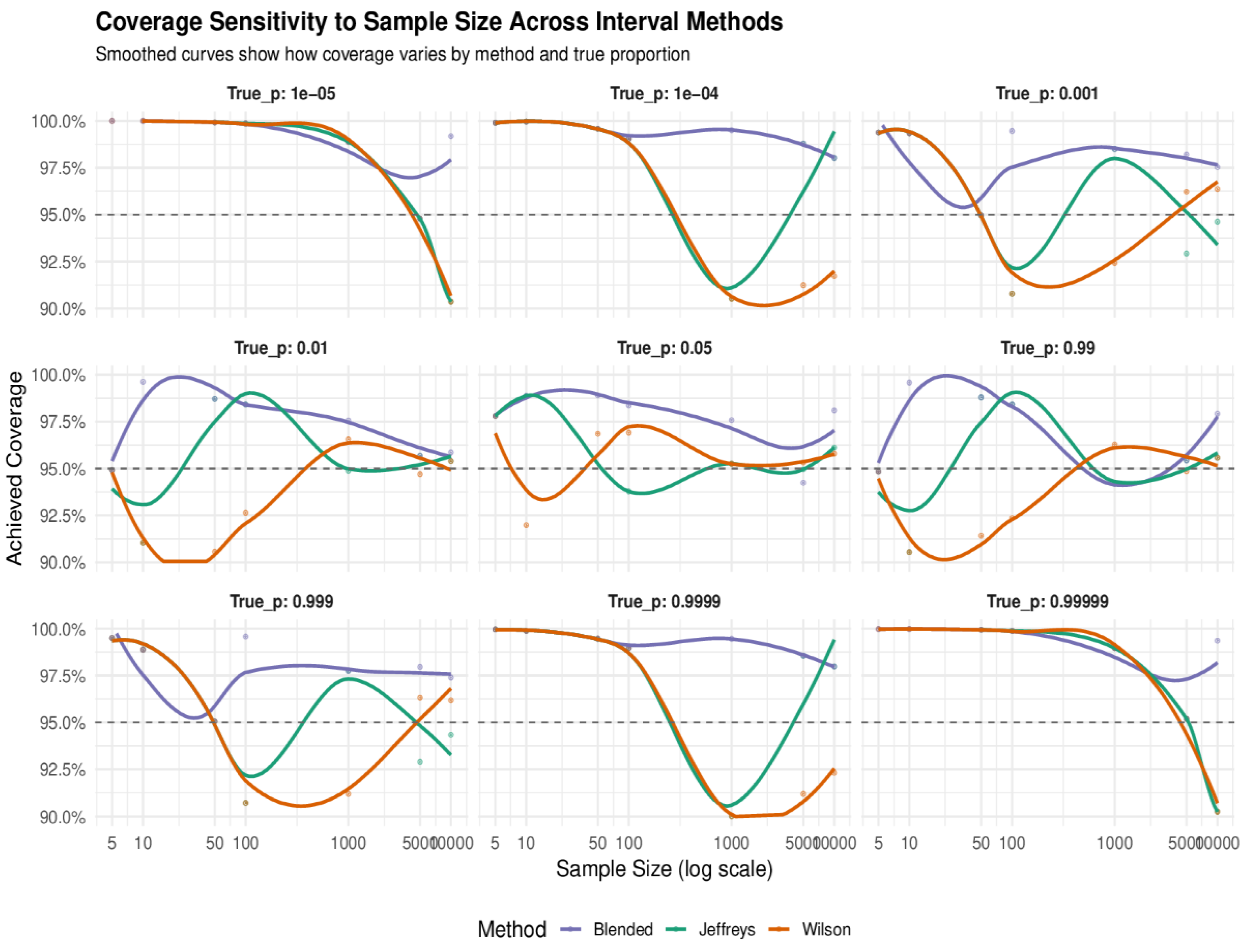
Figure 2.
Credible width across samples.
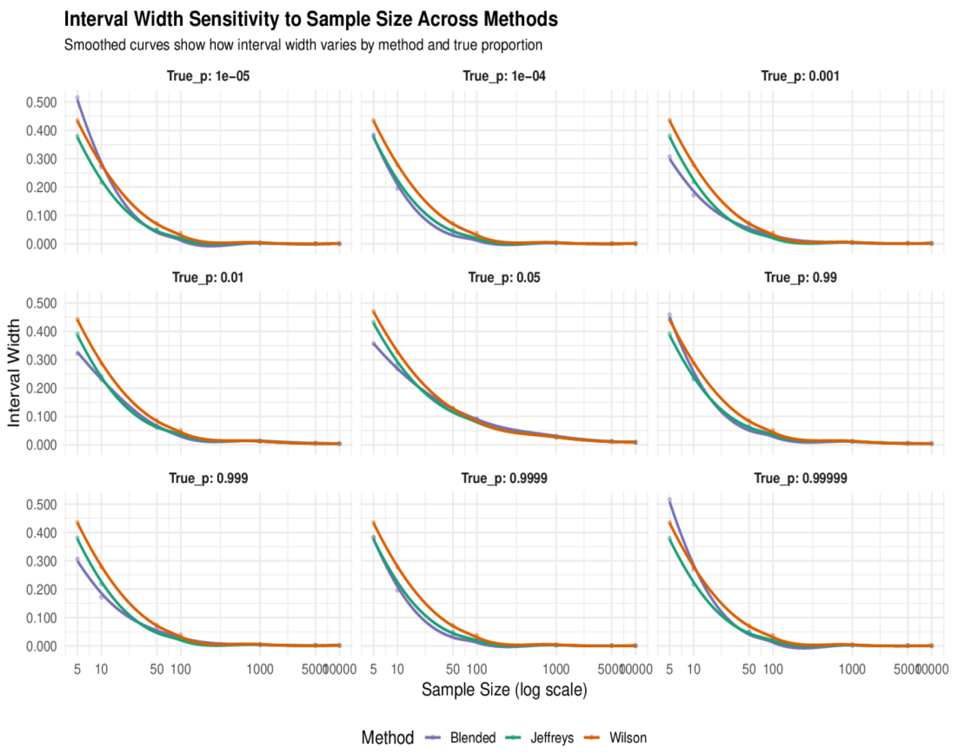
Figure 3.
Sensitivity of tunned credible levels.
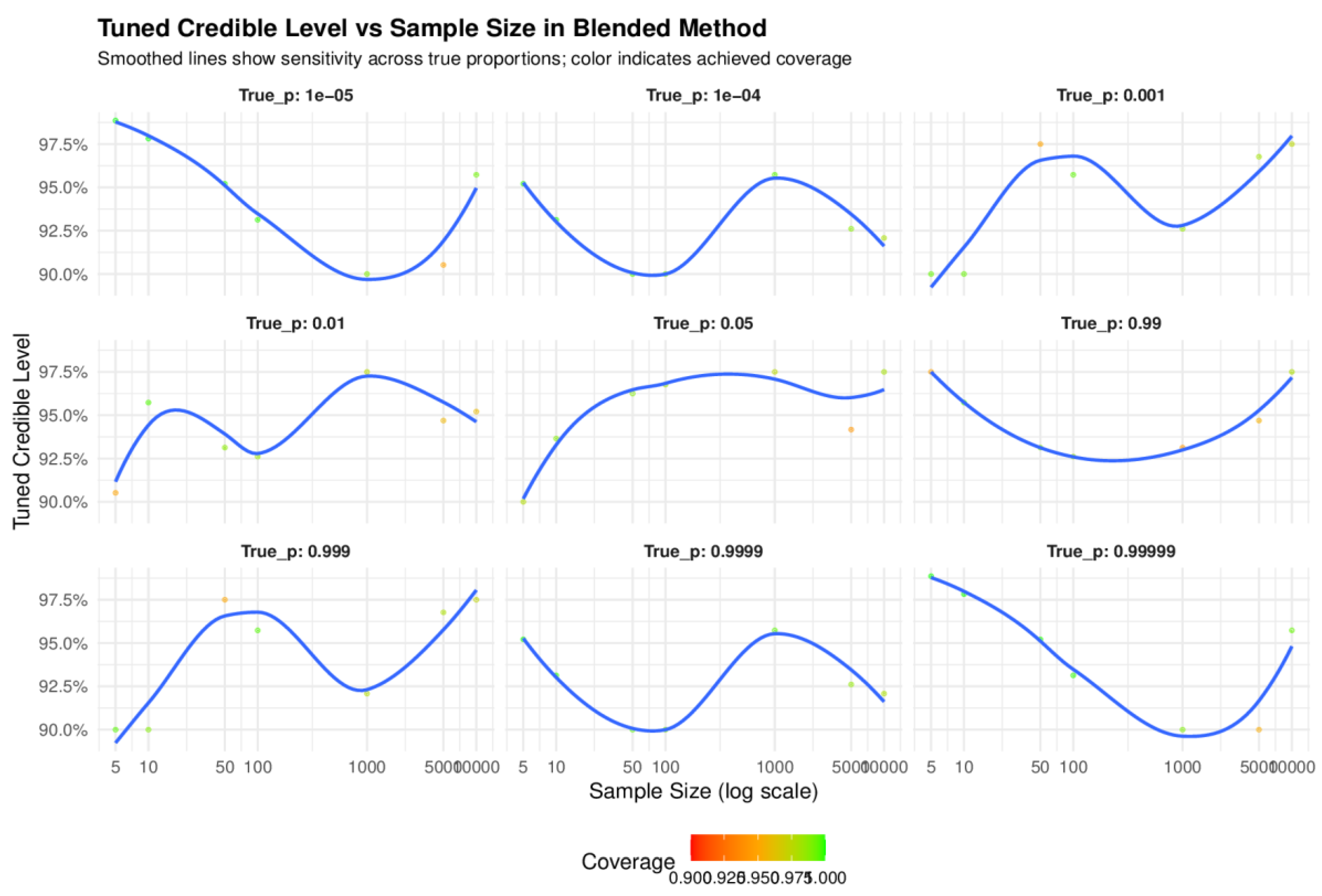

Table 1.
Ultra-Rare Events (True proportion ≤ 0.0001).
| Sample Size | Jeffreys Coverage | WS Coverage | Blend Coverage | Jeffreys Width | WS Width | Blend Width | Blend Level |
| p=0.00001 | |||||||
| 5 | 0.0000 | 1.0000 | 1.0000 | 0.37928 | 0.43448 | 0.51552 | 0.9886 |
| 10 | 0.0000 | 1.0000 | 1.0000 | 0.21715 | 0.27753 | 0.27072 | 0.9782 |
| 50 | 0.9992 | 0.9992 | 0.9992 | 0.04878 | 0.07137 | 0.04949 | 0.9521 |
| 100 | 0.9986 | 0.9986 | 0.9986 | 0.02477 | 0.03702 | 0.02210 | 0.9313 |
| 1000 | 0.9888 | 0.9888 | 0.9888 | 0.00253 | 0.00385 | 0.00194 | 0.9000 |
| 5000 | 0.9478 | 0.9478 | 0.9478 | 0.00052 | 0.00079 | 0.00041 | 0.9052 |
| 10000 | 0.9036 | 0.9036 | 0.9918 | 0.00027 | 0.00040 | 0.00029 | 0.9573 |
| p=0.0001 | |||||||
| 5 | 0.9990 | 0.9990 | 0.9990 | 0.37951 | 0.43464 | 0.38389 | 0.9521 |
| 10 | 0.9996 | 0.9996 | 0.9996 | 0.21721 | 0.27758 | 0.19600 | 0.9313 |
| 50 | 0.9958 | 0.9958 | 0.9958 | 0.04891 | 0.07147 | 0.03761 | 0.9000 |
| 100 | 0.9904 | 0.9904 | 0.9904 | 0.02493 | 0.03714 | 0.01913 | 0.9000 |
| 1000 | 0.9052 | 0.9052 | 0.9950 | 0.00271 | 0.00399 | 0.00285 | 0.9573 |
| 5000 | 0.9878 | 0.9124 | 0.9878 | 0.00069 | 0.00092 | 0.00061 | 0.9261 |
| 10000 | 0.9802 | 0.9172 | 0.9802 | 0.00043 | 0.00053 | 0.00038 | 0.9208 |
Table 2.
Rare Events (0.001 < True proportion ≤ 0.01).
| Sample Size | Jeffreys Coverage | WS Coverage | Blend Coverage | Jeffreys Width | WS Width | Blend Width | Blend Level |
| p=0.001 | |||||||
| 5 | 0.9938 | 0.9938 | 0.9938 | 0.38069 | 0.43544 | 0.30674 | 0.9000 |
| 10 | 0.9934 | 0.9934 | 0.9934 | 0.21816 | 0.27825 | 0.17152 | 0.9000 |
| 50 | 0.9496 | 0.9496 | 0.9496 | 0.05073 | 0.07289 | 0.06232 | 0.9750 |
| 100 | 0.9078 | 0.9078 | 0.9946 | 0.02666 | 0.03851 | 0.02804 | 0.9573 |
| 1000 | 0.9850 | 0.9242 | 0.9850 | 0.00423 | 0.00524 | 0.00378 | 0.9261 |
| 5000 | 0.9292 | 0.9622 | 0.9820 | 0.00177 | 0.00188 | 0.00194 | 0.9677 |
| 10000 | 0.9462 | 0.9636 | 0.9754 | 0.00125 | 0.00128 | 0.00143 | 0.9750 |
| p=0.01 | |||||||
| 5 | 0.9492 | 0.9492 | 0.9492 | 0.39088 | 0.44234 | 0.32265 | 0.9052 |
| 10 | 0.9104 | 0.9104 | 0.9962 | 0.23121 | 0.28753 | 0.24178 | 0.9573 |
| 50 | 0.9872 | 0.9056 | 0.9872 | 0.06687 | 0.08560 | 0.06080 | 0.9313 |
| 100 | 0.9842 | 0.9264 | 0.9842 | 0.04222 | 0.05113 | 0.03782 | 0.9261 |
| 1000 | 0.9488 | 0.9656 | 0.9756 | 0.01236 | 0.01273 | 0.01418 | 0.9750 |
| 5000 | 0.9568 | 0.9470 | 0.9568 | 0.00552 | 0.00555 | 0.00545 | 0.9469 |
| 10000 | 0.9540 | 0.9540 | 0.9586 | 0.00390 | 0.00391 | 0.00394 | 0.9521 |
Table 3.
Events (0.01 < True proportion ≤0.99).
| Sample Size | Jeffreys Coverage | WS Coverage | Blend Coverage | Jeffreys Width | WS Width | Blend Width | Blend Level |
| p=0.05 | |||||||
| 5 | 0.9780 | 0.9780 | 0.9780 | 0.43260 | 0.47068 | 0.35727 | 0.9000 |
| 10 | 0.9888 | 0.9198 | 0.9888 | 0.28586 | 0.32669 | 0.26848 | 0.9365 |
| 50 | 0.8922 | 0.9686 | 0.9890 | 0.11908 | 0.12887 | 0.12683 | 0.9625 |
| 100 | 0.9378 | 0.9692 | 0.9836 | 0.08451 | 0.08831 | 0.09252 | 0.9677 |
| 1000 | 0.9526 | 0.9526 | 0.9758 | 0.02699 | 0.02711 | 0.03087 | 0.9750 |
| 5000 | 0.9496 | 0.9532 | 0.9424 | 0.01209 | 0.01210 | 0.01167 | 0.9417 |
| 10000 | 0.9612 | 0.9580 | 0.9810 | 0.00854 | 0.00854 | 0.00977 | 0.9750 |
| p=0.99 | |||||||
| 5 | 0.9484 | 0.9484 | 0.9484 | 0.39115 | 0.44253 | 0.45849 | 0.9750 |
| 10 | 0.9054 | 0.9054 | 0.9958 | 0.23202 | 0.28811 | 0.24260 | 0.9573 |
| 50 | 0.9880 | 0.9142 | 0.9880 | 0.06617 | 0.08504 | 0.06013 | 0.9313 |
| 100 | 0.9842 | 0.9236 | 0.9842 | 0.04191 | 0.05088 | 0.03753 | 0.9261 |
| 1000 | 0.9420 | 0.9628 | 0.9420 | 0.01237 | 0.01273 | 0.01147 | 0.9313 |
| 5000 | 0.9544 | 0.9486 | 0.9544 | 0.00551 | 0.00554 | 0.00544 | 0.9469 |
| 10000 | 0.9558 | 0.9558 | 0.9792 | 0.00389 | 0.00391 | 0.00446 | 0.9750 |
Table 4.
Extreme Events (True proportion > 0.99).
| Sample Size | Jeffreys Coverage | WS Coverage | Blend Coverage | Jeffreys Width | WS Width | Blend Width | Blend Level |
| p=0.999 | |||||||
| 5 | 0.9950 | 0.9950 | 0.9950 | 0.38042 | 0.43525 | 0.30648 | 0.9000 |
| 10 | 0.9888 | 0.9888 | 0.9888 | 0.21888 | 0.27876 | 0.17219 | 0.9000 |
| 50 | 0.9506 | 0.9506 | 0.9506 | 0.05071 | 0.07287 | 0.06230 | 0.9750 |
| 100 | 0.9072 | 0.9072 | 0.9958 | 0.02665 | 0.03850 | 0.02803 | 0.9573 |
| 1000 | 0.9776 | 0.9120 | 0.9776 | 0.00430 | 0.00530 | 0.00377 | 0.9208 |
| 5000 | 0.9290 | 0.9632 | 0.9796 | 0.00176 | 0.00187 | 0.00193 | 0.9677 |
| 10000 | 0.9434 | 0.9618 | 0.9740 | 0.00124 | 0.00128 | 0.00143 | 0.9750 |
| p=0.9999 | |||||||
| 5 | 0.9996 | 0.9996 | 0.9996 | 0.37937 | 0.43454 | 0.38375 | 0.9521 |
| 10 | 0.9988 | 0.9988 | 0.9988 | 0.21733 | 0.27766 | 0.19612 | 0.9313 |
| 50 | 0.9946 | 0.9946 | 0.9946 | 0.04896 | 0.07151 | 0.03765 | 0.9000 |
| 100 | 0.9896 | 0.9896 | 0.9896 | 0.02495 | 0.03716 | 0.01914 | 0.9000 |
| 1000 | 0.9002 | 0.9002 | 0.9946 | 0.00272 | 0.00400 | 0.00286 | 0.9573 |
| 5000 | 0.9856 | 0.9120 | 0.9856 | 0.00069 | 0.00092 | 0.00061 | 0.9261 |
| 10000 | 0.9798 | 0.9232 | 0.9798 | 0.00043 | 0.00053 | 0.00038 | 0.9208 |
| p=0.99999 | |||||||
| 5 | 0.0000 | 0.9998 | 0.9998 | 0.37933 | 0.43451 | 0.51556 | 0.9886 |
| 10 | 0.0000 | 0.9998 | 0.9998 | 0.21718 | 0.27755 | 0.27075 | 0.9782 |
| 50 | 0.9994 | 0.9994 | 0.9994 | 0.04877 | 0.07137 | 0.04948 | 0.9521 |
| 100 | 0.9988 | 0.9988 | 0.9988 | 0.02476 | 0.03701 | 0.02209 | 0.9313 |
| 1000 | 0.9896 | 0.9896 | 0.9896 | 0.00253 | 0.00384 | 0.00194 | 0.9000 |
| 5000 | 0.9520 | 0.9520 | 0.9520 | 0.00052 | 0.00078 | 0.00040 | 0.9000 |
| 10000 | 0.9026 | 0.9026 | 0.9936 | 0.00027 | 0.00040 | 0.00029 | 0.9573 |
Table 5.
Performance of Interval Estimation Methods for COVID-19 mortality rates.
| Country | Sample size | True P | Jeffreys | Wilson | Blended | Jeffreys | Wilson | Blended |
| Coverage | Width | |||||||
| Western Sahara | 10 | 0.10000 | 0.98733 | 0.92967 | 0.98733 | 0.34371 | 0.36878 | 0.33176 |
| Ghana | 171 889 | 0.00851 | 0.94733 | 0.94633 | 0.97367 | 0.00087 | 0.00087 | 0.00099 |
| South Africa | 4 076 463 | 0.02517 | 0.94633 | 0.94633 | 0.97383 | 0.00030 | 0.00030 | 0.00035 |
| Australia | 11 853 144 | 0.00206 | 0.94550 | 0.94500 | 0.97333 | 0.00005 | 0.00005 | 0.00006 |
| Brazil | 38 743 918 | 0.01836 | 0.94983 | 0.94983 | 0.95150 | 0.00008 | 0.00008 | 0.00009 |
| Germany | 38 828 995 | 0.00471 | 0.94933 | 0.94933 | 0.97283 | 0.00004 | 0.00004 | 0.00005 |
| France | 40 138 560 | 0.00418 | 0.95283 | 0.95283 | 0.97533 | 0.00004 | 0.00004 | 0.00005 |
| USA | 111 820 082 | 0.01091 | 0.95050 | 0.95050 | 0.95267 | 0.00004 | 0.00004 | 0.00004 |
Table 6.
Performance of Interval Estimation Methods for COVID-19 Recovery Rates.
| Country | Sample size | True P | Jeffreys | Wilson | Blended | Jeffreys | Wilson | Blended |
| Coverage | Width | |||||||
| Western Sahara | 10 | 0.77778 | 0.98600 | 0.92683 | 0.98600 | 0.34513 | 0.36977 | 0.33316 |
| Ghana | 171 889 | 0.90000 | 0.95467 | 0.95317 | 0.95983 | 0.00087 | 0.00087 | 0.00090 |
| South Africa | 4 076 463 | 0.99148 | 0.95150 | 0.95150 | 0.95917 | 0.00038 | 0.00038 | 0.00039 |
| Australia | 11 853 144 | 0.95978 | 0.95267 | 0.95267 | 0.97583 | 0.00015 | 0.00015 | 0.00018 |
| Brazil | 38 743 918 | 0.93561 | 0.95067 | 0.95067 | 0.97783 | 0.00004 | 0.00004 | 0.00005 |
| Germany | 38 828 995 | 0.99529 | 0.95733 | 0.95717 | 0.96933 | 0.00004 | 0.00004 | 0.00004 |
| France | 40 138 560 | 0.99582 | 0.95067 | 0.95067 | 0.97383 | 0.00005 | 0.00005 | 0.00006 |
| USA | 111 820 082 | 0.98206 | 0.98600 | 0.92683 | 0.98600 | 0.00005 | 0.00005 | 0.00006 |
Disclaimer/Publisher’s Note: The statements, opinions and data contained in all publications are solely those of the individual author(s) and contributor(s) and not of MDPI and/or the editor(s). MDPI and/or the editor(s) disclaim responsibility for any injury to people or property resulting from any ideas, methods, instructions or products referred to in the content. |
© 2025 by the authors. Licensee MDPI, Basel, Switzerland. This article is an open access article distributed under the terms and conditions of the Creative Commons Attribution (CC BY) license (http://creativecommons.org/licenses/by/4.0/).
Copyright: This open access article is published under a Creative Commons CC BY 4.0 license, which permit the free download, distribution, and reuse, provided that the author and preprint are cited in any reuse.


