Fuzzy, Neutrosophic, and Plithogenic Approaches to Project Scheduling, Multischeduling, and Iterative Multischeduling

1. Preliminaries

This section introduces the fundamental concepts and definitions that underpin the discussions in this paper. Throughout, all sets are assumed to be finite.

1.1. Fuzzy Set and Neutrosophic Set

A fuzzy set assigns to each element a grade in the interval $[0,1]$, thereby representing uncertainty by degrees rather than by a strict binary split [1,2,3]. Related concepts include the Bipolar Fuzzy Set [4,5], the Spherical Fuzzy Set [6,7,8], the Picture Fuzzy Set [9,10], the Shadowed Set [11,12], and the m-polar Fuzzy Set [13]. Below we recall the relevant notions, together with their extensions.

Definition 1  

(Fuzzy Set). [1,14] Let Y be a nonempty universe. A fuzzy set on Y is a mapping $\tau :Y\to [0,1]$. A fuzzy relation on Y is a fuzzy subset $\delta :Y\times Y\to [0,1]$. We say that δ is a fuzzy relation onτ if, for all $y,z\in Y$,

$$\delta (y,z)\le min\left\{\tau \right(y),\tau (z\left)\right\}.$$

Example 1  

(Fuzzy set in project management: uncertain task duration). Let $Y={\mathbb{R}}_{\ge 0}$ denote possible durations (days) of a software testing task. Model the expert estimate “about 10 days, realistically between 8 and 14” by the triangular fuzzy set $\tau :Y\to [0,1]$ with

$$\tau \left(t\right)=\left\{\begin{array}{cc}0,\hfill & t<8,\hfill \\ {\displaystyle \frac{t-8}{10-8}},\hfill & 8\le t\le 10,\hfill \\ {\displaystyle \frac{14-t}{14-10}},\hfill & 10<t\le 14,\hfill \\ 0,\hfill & t>14.\hfill \end{array}\right.$$

Here $\tau \left(9\right)=0.5$ expresses a moderate plausibility of finishing in 9 days, while $\tau \left(12\right)=0.5$ quantifies a similar plausibility for 12 days. Such fuzzy durations can be propagated through a precedence network via Zadeh’s extension principle to compute fuzzy earliest/finish times and support time–cost tradeoffs under uncertainty.

Neutrosophic sets extend fuzzy sets by explicitly incorporating indeterminacy, thus covering statements that are neither entirely true nor entirely false, and offering a flexible representation of ambiguity [15,16,17,18]. Related concepts include the Bipolar Neutrosophic Set, the Hesitant Neutrosophic Set [19,20,21], Neutrosophic Rough Set [22,23,24], the Neutrosophic Cubic Set [25,26,27], the Complex Neutrosophic Set [28,29], and the Interval-Valued Neutrosophic Set [30,31,32]. Their formal specification is as follows.

Definition 2  

(Neutrosophic Set). [15,33] Let X be a nonempty set. A Neutrosophic Set (NS)A on X is determined by three functions

$$T_A:X\to [0,1],I_A:X\to [0,1],F_A:X\to [0,1],$$

where, for each $x\in X$, $T_A\left(x\right)$, $I_A\left(x\right)$, and $F_A\left(x\right)$ denote the degrees of truth, indeterminacy, and falsity, respectively. These values satisfy

$$0\le T_A\left(x\right)+I_A\left(x\right)+F_A\left(x\right)\le 3.$$

Example 2  

(Neutrosophic set in project management: on-time supplier delivery). Let $X=\{\mathrm{A},\mathrm{B}\}$ be two hardware suppliers and consider the statement “deliver the batch by Day 20.” Represent each supplier by a single-valued neutrosophic triple $(T,I,F)\in {[0,1]}^3$ capturing, respectively, the degrees of truth, indeterminacy, and falsity for that statement:

$$\mathit{Supplier}\mathrm{A}:(T,I,F)=(0.75,0.15,0.10),\mathit{Supplier}\mathrm{B}:(T,I,F)=(0.55,0.30,0.15).$$

Supplier A has stronger supporting evidence ($T=0.75$) and less conflict ($F=0.10$), with moderate ambiguity ($I=0.15$); Supplier B is less convincing and more ambiguous. These triples let the project manager rank or threshold suppliers while explicitly accounting for conflicting information and residual indeterminacy in the schedule risk assessment.

Neutrosophic Sets have been extensively studied in the field of project management [34,35,36,37,38,39,40]. These studies demonstrate how neutrosophic logic effectively models uncertainty, inconsistency, and incompleteness in project evaluation, scheduling, and decision-making processes.

1.2. Plithogenic Set

A plithogenic set [41,42,43,44,45,46] represents elements via membership driven by explicit attributes together with a contradiction mapping between attribute values, thereby subsuming and extending the frameworks of Fuzzy [1,47], Vague [48], Intuitionistic [49,50], Hesitant Fuzzy Set [51,52], and Neutrosophic sets [16,17,53].

Definition 3  

(Plithogenic Set). [41,54] Let S be a universe and $P\subseteq S$ a nonempty subset. A plithogenic set is a 5–tuple

$$PS=(P,v,Pv,pdf,pCF),$$

with the following ingredients:

• v — a chosen attribute;
• $Pv$ — the value domain of v;
• $pdf:P\times Pv\to {[0,1]}^s$ — the degree of appurtenance(DAF);1
• $pCF:Pv\times Pv\to {[0,1]}^t$ — the degree of contradiction(DCF).

For every $a,b\in Pv$, the DCF satisfies

$$\mathit{reflexivity}:pCF(a,a)=0,\mathit{symmetry}:pCF(a,b)=pCF(b,a).$$

Here $s,t\in \mathbb{N}$ are, respectively, the appurtenance and contradiction dimensions.

Example 3  

(Plithogenic set in project management: sprint plan under attribute contradiction). Let $P=\{{\mathit{Plan}}_1,{\mathit{Plan}}_2\}$ be two sprint plans for a six-week release. Choose the attribute $v=``\mathit{risk}\mathit{level}’’$ with value domain $Pv=\{\mathit{low},\mathit{medium},\mathit{high}\}$. Use a (scalar) degree-of-appurtenance $pdf:P\times Pv\to [0,1]$ to encode how strongly each plan fits “feasible within 6 weeks” under each risk value: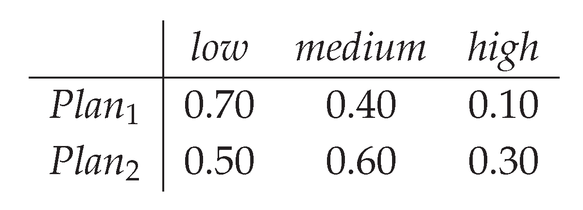

Specify a symmetric degree-of-contradiction $pCF:Pv\times Pv\to [0,1]$ with

$$pCF(\mathit{low},\mathit{low})=pCF(\mathit{medium},\mathit{medium})=pCF(\mathit{high},\mathit{high})=0,$$

$$pCF(\mathit{low},\mathit{medium})=0.30,pCF(\mathit{medium},\mathit{high})=0.60,pCF(\mathit{low},\mathit{high})=1.00,$$

and $pCF(a,b)=pCF(b,a)$. The pair $\left(pdf,pCF\right)$ constitutes a plithogenic description of feasibility: attributes with stronger mutual contradiction (e.g., “low” vs. “high” risk) are penalized more by the plithogenic aggregation. A manager can aggregate these values to obtain an effective feasibility for each plan that respects both membership strengths and inter-value contradictions, then select the plan with the higher effective feasibility.

1.3. Multi-Structure

A Multi-Structure replaces classical operations with maps from tuples to finite multisets, enabling multiple outputs per input tuple flexibly simultaneously [56,57,58,59].

Definition 4  

(Finite Multiset). (cf.[60,61,62,63]) Let H be a nonempty set. A finite multiset on H is a function

$$m:H⟶{\mathbb{N}}_0$$

with finite support $\{x\in H\mid m(x)>0\}$. We denote by $\mathcal{M}\left(H\right)$ the collection of all such finite multisets on H. Equivalently, an element of $\mathcal{M}\left(H\right)$ can be written as $\{x_1^{k_1},x_2^{k_2},\dots ,x_r^{k_r}\}$, where each $x_i\in H$ and $k_i=m\left(x_i\right)\in \mathbb{N}$.

Definition 5  

(MultiOperation). Let H be a nonempty set and fix an integer $m\ge 1$. A multi-operation of arity m on H is a map

$${\#}^{\left(m\right)}:H^m⟶\mathcal{M}\left(H\right),$$

$$(x_1,\dots ,x_m)\mapsto {\#}^{\left(m\right)}(x_1,\dots ,x_m)\in \mathcal{M}\left(H\right).$$

Thus, instead of producing a single element of H, a multi-operation assigns a finite multiset of elements of H.

Definition 6  

(MultiStructure). A MultiStructure is a pair

$$\mathcal{MS}=\left(H,{\{{\#}^{\left(m\right)}:H^m\to \mathcal{M}\left(H\right)\}}_{m\in \mathcal{I}}\right),$$

where H is a nonempty carrier set and $\mathcal{I}\subseteq {\mathbb{Z}}_{>0}$ indexes a family of multi-operations of various arities. No further axioms are imposed unless specified.

Example 4  

(Multi-Structure in everyday project planning: combining schedule proposals). Let $H={\mathbb{R}}_{\ge 0}^3$ denote start times (in days) for three tasks. Given two proposed schedules $x=(0,3,6)$ and $y=(1,4,5)$, define the binary multi-operation ${\#}^{\left(2\right)}:H^2\to \mathcal{M}\left(H\right)$ by three concrete combiners:

$$A_{min}(x,y)={min}_{\mathit{coord}}(x,y),A_{max}(x,y)={max}_{\mathit{coord}}(x,y),A_{\mathit{avg}}(x,y)=\frac{1}{2}(x+y).$$

Then

$${\#}^{\left(2\right)}(x,y)=\left\{A_{min}(x,y),A_{max}(x,y),A_{\mathit{avg}}(x,y)\right\}=\left\{(0,3,5),(1,4,6),(0.5,3.5,5.5)\right\}\in \mathcal{M}\left(H\right).$$

Thus a single pair of inputs produces a finite multiset of candidate schedules: an aggressive timeline (min), a conservative one (max), and a compromise ($\mathit{avg}$). This models a common meeting where two teams propose timelines and the planner keeps multiple viable variants simultaneously.

1.4. Iterative Multi-Structure

An Iterative Multi-Structure extends multiset operations across levels, combining multisets of multisets iteratively through k hierarchical stages in layered aggregation [64,65].

Definition 7  

(Iterative Multi-Structure of Order k). Let H be a nonempty set and fix an integer $k\ge 1$. Define iteratively the multiset powersets

$${\mathcal{M}}^0\left(H\right)=H,{\mathcal{M}}^{i+1}\left(H\right)=\mathcal{M}\left({\mathcal{M}}^i\left(H\right)\right),i=0,1,\dots ,k-1,$$

where $\mathcal{M}\left(X\right)$ denotes the collection of finite multisets on X (Definition 4). Let $\mathcal{I}\subseteq {\mathbb{Z}}_{>0}$ index a family of arities. An Iterative Multi-Structure of order kis a tuple

$${\mathcal{IMS}}^{\left(k\right)}=\left(H,{\left\{{\#}^{(m,i)}:{\left({\mathcal{M}}^i\left(H\right)\right)}^m⟶{\mathcal{M}}^{i+1}\left(H\right)\right\}}_{m\in \mathcal{I},0\le i<k}\right),$$

where for each $i=0,\dots ,k-1$ and each $m\in \mathcal{I}$,

$${\#}^{(m,i)}(x_1,\dots ,x_m)\in {\mathcal{M}}^{i+1}\left(H\right),x_j\in {\mathcal{M}}^i\left(H\right).$$

Thus ${\#}^{(m,0)}$ is an ordinary Multi-Structure operation on H, ${\#}^{(m,1)}$ combines multisets of multisets, and so on, up to level k.

Example 5  

(Iterative Multi-Structure in practice: two-level portfolio scheduling). Consider a company release involving two departments, Marketing (M) and Engineering (E). Let $H={\mathbb{R}}_{\ge 0}^2$ be start times for two key milestones. Each department supplies two proposals:

$$x_1^{\mathrm{M}}=(0,2),x_2^{\mathrm{M}}=(1,1.5),x_1^{\mathrm{E}}=(0.5,1.8),x_2^{\mathrm{E}}=(0.2,2.2).$$

Level 0 (within-department mixing).  Define ${\#}^{(2,0)}:H^2\to \mathcal{M}\left(H\right)$ using the three combiners from the previous example. For Marketing,

$$M_0={\#}^{(2,0)}\left(x_1^{\mathrm{M}},x_2^{\mathrm{M}}\right)=\left\{(0,1.5),(1,2),(0.5,1.75)\right\}\in \mathcal{M}\left(H\right).$$

For Engineering,

$$E_0={\#}^{(2,0)}\left(x_1^{\mathrm{E}},x_2^{\mathrm{E}}\right)=\left\{(0.2,1.8),(0.5,2.2),(0.35,2.0)\right\}\in \mathcal{M}\left(H\right).$$

Level 1 (cross-department aggregation).  Define ${\#}^{(2,1)}:{\left(\mathcal{M}\left(H\right)\right)}^2\to \mathcal{M}\left(\mathcal{M}\left(H\right)\right)$ by the combiner

$$A_{max}^{\left(1\right)}(M_0,E_0)=\left\{{max}_{\mathit{coord}}(m,e):m\in supp\left(M_0\right),e\in supp\left(E_0\right)\right\},$$

collecting every coordinatewise-feasible portfolio schedule. Hence

$${\#}^{(2,1)}(M_0,E_0)=\left\{A_{max}^{\left(1\right)}(M_0,E_0)\right\}\in \mathcal{M}\left(\mathcal{M}\left(H\right)\right),$$

which is a multiset of multisets(each inner multiset is a finite set of combined schedules). Flattening by Unnest (as defined elsewhere) yields a finite multiset of portfolio schedules in H. This two-level construction is an Iterative Multi-Structure of order $k=2$: level 0 mixes proposals within departments; level 1 aggregates department-level results into company-level candidates, reflecting a common real workflow in release planning.

1.5. Project Scheduling and Fuzzy Project Scheduling

Project scheduling assigns start/finish times to interdependent activities on a precedence network to optimize overall duration, cost, and resource usage [66,67,68,69,70,71]. Fuzzy project scheduling represents uncertain activity durations by fuzzy numbers, optimizing network objectives using expected values or credibility-constrained mathematical approaches [72,73,74,75,76,77,78].

Definition 8 (Project Scheduling (deterministic)). Let a project be represented by a directed acyclic graph $G=(V,A)$ with source 1 and sink $n+1$. Each arc $(i,j)\in A$ is an activity of deterministic duration $d_{ij}>0$ and cost $c_{ij}\ge 0$. For decision vector $x=(x_1,\dots ,x_n)$ (e.g., release/start or funding times), define node start times $T_i(x,d)$ by

$$T_1(x,d)=x_1,T_i(x,d)\ge x_i,T_i(x,d)\ge \underset{(k,i)\in A}{max}\left\{T_k(x,d)+d_{ki}\right\}(i=2,\dots ,n),$$

and project completion time

$$T(x,d)=\underset{(k,n+1)\in A}{max}\left\{T_k(x,d)+d_{k,n+1}\right\}.$$

If financing accrues at rate $r\ge 0$, the total cost is

$$C(x,d)=\sum _{(i,j)\in A}{c}_{ij}{(1+r)}^{\lceil T(x,d)-x_i\rceil }.$$

The (deterministic) project scheduling problem is

$$\underset{x}{min}C(x,d)\mathrm{s}.\mathrm{t}.T(x,d)\le T_0,x\ge 0\left(\mathit{integer}\mathit{or}\mathit{continuous}\mathit{as}\mathit{modeled}\right).$$

This captures the classical tradeoff between completion time and total cost.

Example 6  

(Project Scheduling in practice: office renovation with a critical path). Consider an office renovation with tasks arranged as a DAG $G=(V,A)$:

$$V=\{1,2,3,4,5\}(\mathit{source}1,\mathit{sin}\mathrm{k}5),A=\{(1,2),(2,3),(2,4),(3,5),(4,5)\}.$$

Interpretation: $(1,2)$ “permit approval”, $(2,3)$ “demolition”, $(2,4)$ “electrical & HVAC”, $(3,5)$ “finishes”, $(4,5)$ “inspection & handover”. Durations (days) and costs (k$) are deterministic:

$$d_{1,2}=4,c_{1,2}=100;d_{2,3}=3,c_{2,3}=120;d_{2,4}=2,c_{2,4}=80;d_{3,5}=2,c_{3,5}=150;d_{4,5}=5,c_{4,5}=90.$$

Choose start vector $x=(x_1,x_2,x_3,x_4)=(0,0,0,0)$. Then

$$T_2=max\{x_2,T_1+d_{1,2}\}=max\{0,0+4\}=4,T_3=max\{x_3,T_2+d_{2,3}\}=max\{0,4+3\}=7,$$

$$T_4=max\{x_4,T_2+d_{2,4}\}=max\{0,4+2\}=6,T(x,d)=max\{T_3+d_{3,5},T_4+d_{4,5}\}=max\{7+2,6+5\}=11.$$

Thus the critical path is $1\to 2\to 4\to 5$ with project completion time 11 days. If financing accrues at $r=0.05$, the total cost is

$$C(x,d)=\sum _{(i,j)\in A}{c}_{ij}{(1+r)}^{\lceil T(x,d)-x_i\rceil }={\left(1.05\right)}^{11}(100+120+80+150+90).$$

This mirrors a real renovation: parallel trades (demolition vs. MEP work) and a longer inspection stage determine the finish date and the capitalized cost.

Definition 9  

(Fuzzy Project Scheduling). Assume each activity duration is a fuzzy quantity ${\tilde{n}}_{ij}$ (e.g., a trapezoidal fuzzy number) on the same network $G=(V,A)$. Let $T_i(x,\tilde{n})$, $T(x,\tilde{n})$ and $C(x,\tilde{n})$ be the induced fuzzy start time, completion time, and cost. Using the credibility measure $Cr\{·\}$ and fuzzy expectation $\mathbb{E}[·]$, three concise formulations are standard:

$$\begin{array}{cccc}\hfill \left(\mathbf{EVM}\right)& \underset{x}{min}\mathbb{E}\left[C(x,\tilde{n})\right]\hfill & \hfill & \mathrm{s}.\mathrm{t}.\mathbb{E}\left[T(x,\tilde{n})\right]\le T_0,x\ge 0;\hfill \\ \hfill (\alpha -\mathbf{cost})& \underset{x,C_0}{min}{C}_0\hfill & \hfill & \mathrm{s}.\mathrm{t}.Cr\left\{C(x,\tilde{n})\le C_0\right\}\ge \alpha ,Cr\left\{T(x,\tilde{n})\le T_0\right\}\ge \beta ,x\ge 0;\hfill \\ \hfill \left(\mathbf{Credibility}\mathbf{max}\right)& \underset{x}{max}Cr\left\{C(x,\tilde{n})\le C_0\right\}\hfill & \hfill & \mathrm{s}.\mathrm{t}.Cr\left\{T(x,\tilde{n})\le T_0\right\}\ge \alpha ,x\ge 0.\hfill \end{array}$$

These formulations are widely used to balance time and cost under fuzzy activity times via credibility/chance constraints and fuzzy expectation.

Example 7  

(Fuzzy Project Scheduling in practice: software release under uncertain task times). Re-use the same network $G=(V,A)$ but model activity durations by triangular fuzzy numbers (TFNs):

$${\tilde{n}}_{1,2}=\mathit{TFN}(3.5,4,4.5),{\tilde{n}}_{2,3}=\mathit{TFN}(2.5,3,3.5),{\tilde{n}}_{2,4}=\mathit{TFN}(1.5,2,2.5),$$

$${\tilde{n}}_{3,5}=\mathit{TFN}(1.5,2,2.5),{\tilde{n}}_{4,5}=\mathit{TFN}(4.5,5,5.5).$$

These represent, for a software release, uncertain durations for “requirements approval”, “refactor legacy”, “infrastructure & CI”, “UI polish”, and “security review”. Using Zadeh’s extension principle, the fuzzy completion time $\tilde{T}(x,\tilde{n})$ is induced from path sums and the network max. For planning, apply centroid defuzzification $\mathit{cen}\left(\mathit{TFN}\right(a,b,c\left)\right)=(a+b+c)/3$ to approximate expected durations:

$$\mathbb{E}\left[{\tilde{n}}_{1,2}\right]=4,\mathbb{E}\left[{\tilde{n}}_{2,3}\right]=3,\mathbb{E}\left[{\tilde{n}}_{2,4}\right]=2,\mathbb{E}\left[{\tilde{n}}_{3,5}\right]=2,\mathbb{E}\left[{\tilde{n}}_{4,5}\right]=5.$$

Hence the expected path lengths are

$$\mathbb{E}[1\to 2\to 3\to 5]=4+3+2=9,\mathbb{E}[1\to 2\to 4\to 5]=4+2+5=11,$$

so the latter remains the (expected) critical path with $\mathbb{E}\left[\tilde{T}\right]=11$. If a budget accrual uses the same $r=0.05$, an expected-cost proxy is

$$\mathbb{E}\left[C(x,\tilde{n})\right]\approx {\left(1.05\right)}^{\mathbb{E}\left[\tilde{T}\right]}(100+120+80+150+90)={\left(1.05\right)}^{11}·540.$$

Decision-makers can also impose credibility constraints, e.g. require $Cr\{\tilde{T}\le T_0\}\ge \beta$, to certify release dates at a chosen confidence level while comparing candidate schedules.

2. Main Results

This section presents the main results of the paper.

2.1. Neutrosophic Project Scheduling

Neutrosophic Project Scheduling models activity durations as Single-Valued Neutrosophic Numbers (SVNNs), propagating truth, indeterminacy, and falsity through the project network under credibility and expectation constraints. Several research works have investigated the Neutrosophic Set from the perspective of Project Scheduling, highlighting its capability to handle incomplete, inconsistent, and uncertain temporal information in practical project management scenarios (cf.[79,80,81,82]).

(NPS)).Definition 10 (Neutrosophic Project Scheduling Let the project network be a finite DAG $G=(V,A)$ with source 1 and sink $n+1$. For each activity $(i,j)\in A$, its duration is modeled by a single-valued neutrosophic number

$${\tilde{n}}_{ij}=(T_{ij},I_{ij},F_{ij}),T_{ij},I_{ij},F_{ij}:{\mathbb{R}}_{\ge 0}\to [0,1],$$

where $T_{ij}\left(x\right)$, $I_{ij}\left(x\right)$, and $F_{ij}\left(x\right)$ denote the degrees of truth, indeterminacy, and falsity for the statement “the duration equals x”. For a decision vector $x=(x_1,\dots ,x_n)$ of planned release/start times, define the neutrosophic start times${\tilde{T}}_i(x,\tilde{n})$ and the neutrosophic completion time$\tilde{T}(x,\tilde{n})$ as single-valued neutrosophic numbers on ${\mathbb{R}}_{\ge 0}$ obtained by Zadeh’s extension principle applied componentwise to the operators $(u,v)\mapsto u+v$ and $(u,v)\mapsto max\{u,v\}$:

$${\tilde{T}}_1(x,\tilde{n})=\widetilde{x_1},{\tilde{T}}_i(x,\tilde{n})⪰\widetilde{x_i},{\tilde{T}}_i(x,\tilde{n})⪰\underset{(k,i)\in A}{max}\left({\tilde{T}}_k(x,\tilde{n})+{\tilde{n}}_{ki}\right),$$

$$\tilde{T}(x,\tilde{n})=\underset{(k,n+1)\in A}{max}\left({\tilde{T}}_k(x,\tilde{n})+{\tilde{n}}_{k,n+1}\right).$$

(Here “+” and “max” act via the extension principle on each of $T,I,F$; the symbol ⪰ indicates the induced partial order on neutrosophic numbers.) Let ${\mathit{Cr}}_{\mathrm{N}}$ be a neutrosophic credibility that assigns to each neutrosophic event E a value in $[0,1]$, and let ${\mathbb{E}}_{\mathrm{N}}[·]$ be a compatible neutrosophic expectation functional. Given targets $T_0>0$, $\alpha ,\beta \in (0,1]$, and a (possibly neutrosophic) cost functional $\tilde{C}(x,\tilde{n})$, the NPS problem is any of the following equivalent chance/expectation formulations:

$$\begin{array}{cccccc}\hfill (\mathbf{N}-\mathbf{cred})& \underset{x,C_0}{min}\hfill & \hfill & C_0\hfill & \hfill & \mathrm{s}.\mathrm{t}.{\mathit{Cr}}_{\mathrm{N}}\left\{\tilde{T}(x,\tilde{n})\le T_0\right\}\ge \beta ,{\mathit{Cr}}_{\mathrm{N}}\left\{\tilde{C}(x,\tilde{n})\le C_0\right\}\ge \alpha ,x\ge 0;\hfill \\ \hfill (\mathbf{N}-\mathbf{exp})& \underset{x}{min}\hfill & \hfill & {\mathbb{E}}_{\mathrm{N}}\left[\tilde{C}(x,\tilde{n})\right]\hfill & \hfill & \mathrm{s}.\mathrm{t}.{\mathbb{E}}_{\mathrm{N}}\left[\tilde{T}(x,\tilde{n})\right]\le T_0,x\ge 0.\hfill \end{array}$$

Example 8  

(Neutrosophic Project Scheduling — Hospital Renovation). A hospital renovates an operating theatre over three serial activities on a DAG $G=(V,A)$ with $V=\{1,2,3,4\}$ and $A=\left\{\right(1,2),(2,3),(3,4\left)\right\}$: demolition $(1,2)$, HVAC installation $(2,3)$, and inspection $(3,4)$. Each activity duration is modeled by a single–valued neutrosophic number ${\tilde{n}}_{ij}=(T_{ij},I_{ij},F_{ij})$ (time in days). For demolition,

$$T_{12}\left(x\right)=max\{0,1-|x-5\left|\right\},I_{12}\left(x\right)=0.2\mathit{for}x\in [4,6],0\mathit{elsewhere},F_{12}\left(x\right)=1-T_{12}\left(x\right),$$

so the most plausible duration is 5 days with small indeterminacy (permits, hidden pipes). Similarly,

$$T_{23}\left(x\right)=max\{0,1-|x-6\left|\right\},I_{23}\left(x\right)=0.15\mathit{on}[5,7],F_{23}\left(x\right)=1-T_{23}\left(x\right),$$

$$T_{34}\left(x\right)=max\{0,1-|x-3\left|\right\},I_{34}\left(x\right)=0.1\mathit{on}[2,4],F_{34}\left(x\right)=1-T_{34}\left(x\right).$$

Given planned releases $x=(x_1,x_2,x_3)$, neutrosophic node times ${\tilde{T}}_i(x,\tilde{n})$ and completion time

$$\tilde{T}(x,\tilde{n})={\tilde{T}}_3(x,\tilde{n})\oplus {\tilde{n}}_{34}$$

are obtained by the componentwise extension of + and max (sup–min for T and its duals for $I,F$). Management sets a target deadline $T_0=16$ days and requires

$${Cr}_{\mathrm{N}}\left\{\tilde{T}(x,\tilde{n})\le T_0\right\}\ge 0.80,$$

while minimizing a neutrosophic expected cost ${\mathbb{E}}_{\mathrm{N}}\left[\tilde{C}(x,\tilde{n})\right]$ (e.g., overtime penalties if the project extends). The scheduler chooses start times $x^{★}$ satisfying the credibility constraint and achieving the smallest ${\mathbb{E}}_{\mathrm{N}}\left[\tilde{C}(x,\tilde{n})\right]$, explicitly accounting for truth, indeterminacy, and falsity in each activity’s duration.

Theorem 1  

(NPS generalizes fuzzy project scheduling). Assume each fuzzy duration ${\tilde{n}}_{ij}^{\mathrm{F}}$ is given by a membership ${\mu }_{ij}:{\mathbb{R}}_{\ge 0}\to [0,1]$. Embed fuzzy numbers into neutrosophic numbers via

$${\iota }_{\mathrm{F}\to \mathrm{N}}:{\tilde{n}}_{ij}^{\mathrm{F}}\mapsto {\tilde{n}}_{ij}=\left(T_{ij},I_{ij},F_{ij}\right),T_{ij}={\mu }_{ij},I_{ij}\equiv 0,F_{ij}=1-{\mu }_{ij}.$$

Let ${\mathit{Cr}}_{\mathrm{N}}$ and ${\mathbb{E}}_{\mathrm{N}}$ reduce on such embeddings to the fuzzy credibility $\mathit{Cr}$ and the fuzzy expectation $\mathbb{E}$ computed from T (i.e. for any fuzzy event A, ${\mathit{Cr}}_{\mathrm{N}}\left(A^{\mathrm{N}}\right)=\mathit{Cr}\left(A\right)$ and ${\mathbb{E}}_{\mathrm{N}}\left[{\tilde{Z}}^{\mathrm{N}}\right]=\mathbb{E}\left[\tilde{Z}\right]$). Then, under the componentwise extension principle, the feasible set and optimal value of NPS coincide with those of the corresponding fuzzy project scheduling problem.

Proof. 

By construction, the T–components of ${\tilde{T}}_i(x,\tilde{n})$ and $\tilde{T}(x,\tilde{n})$ are exactly the fuzzy start/finish-time membership functions obtained by applying Zadeh’s extension principle to $(+,max)$ with inputs ${\mu }_{ij}$. Since $I\equiv 0$ and $F=1-T$ are preserved by the same principle on these embeddings, every neutrosophic event of the form $\{\tilde{Z}\le z\}$ produces T–marginals identical to the fuzzy event membership for $\{Z\le z\}$. By the reduction property of ${\mathit{Cr}}_{\mathrm{N}}$ and ${\mathbb{E}}_{\mathrm{N}}$, the chance and expectation constraints in (N-cred) and (N-exp) coincide with their fuzzy counterparts. Therefore the feasible region and objective values are the same in both models, proving that NPS strictly generalizes fuzzy project scheduling. □

2.2. Plithogenic Project Scheduling

Plithogenic Project Scheduling represents activity durations via attribute-driven memberships and contradiction degrees, aggregating to fuzzy or neutrosophic times for optimization.

(PPS)).Definition 11 (Plithogenic Project Scheduling Retain the network $G=(V,A)$. For each activity $(i,j)\in A$, let its duration be described by a plithogenic description

$${\tilde{p}}_{ij}=\left(pd{f}_{ij},pC{F}_{ij}\right),$$

where $pd{f}_{ij}:{\mathbb{R}}_{\ge 0}\times Pv\to {[0,1]}^s$ gives the degree(s) of appurtenance at duration x for each attribute value $a\in Pv$, and $pC{F}_{ij}:Pv\times Pv\to {[0,1]}^t$ is the degree of contradiction. Let ${\mathcal{A}}_{pCF}$ be a plithogenic aggregation operator that, for each x, merges $\{pd{f}_{ij}(x,a):a\in Pv\}$ into either:

(i) 

an effective fuzzy membership${\mu }_{ij}^{\mathit{eff}}\left(x\right)\in [0,1]$, or

(ii) 

an effective neutrosophic triple$(T_{ij}^{\mathit{eff}},I_{ij}^{\mathit{eff}},F_{ij}^{\mathit{eff}})\left(x\right)\in {[0,1]}^3$,

consistently across x and $(i,j)$.

• Fuzzy-aggregated PPS:If (i) is chosen, define fuzzy start/finish membership by the extension principle on $(+,max)$ using ${\mu }_{ij}^{\mathit{eff}}$, and solve the fuzzy chance/expectation model with credibility $\mathit{Cr}$ and expectation $\mathbb{E}$.
• Neutrosophic-aggregated PPS:If (ii) is chosen, define neutrosophic start/finish numbers via componentwise extension on $(+,max)$ using $(T_{ij}^{\mathit{eff}},I_{ij}^{\mathit{eff}},F_{ij}^{\mathit{eff}})$, and solve the NPS model with ${\mathit{Cr}}_{\mathrm{N}}$ and ${\mathbb{E}}_{\mathrm{N}}$.

In both cases, call the resulting optimization problem the PPS problem(with the chosen aggregation mode).

Example 9  

(Plithogenic Project Scheduling — Coastal Bridge Repair). A coastal bridge repair project faces attribute–dependent durations due to weather. Let the attribute be $v=\mathit{weather}$ with value domain $Pv=\{\mathit{dry},\mathit{stormy}\}$. For the critical activity “deck resurfacing” $(i,j)$ (hours), the plithogenic duration is

$${\tilde{n}}_{ij}=\left(pd{f}_{ij}(·;\mathit{dry}),pd{f}_{ij}(·;\mathit{stormy})\right),$$

with (componentwise) degrees of appurtenance

$$pd{f}_{ij}(x;\mathit{dry})=max\{0,1-|x-10|/2\},pd{f}_{ij}(x;\mathit{stormy})=max\{0,1-|x-14|/3\}.$$

Contradiction between weather values is encoded by

$$pCF(\mathit{dry},\mathit{stormy})=pCF(\mathit{stormy},\mathit{dry})=0.8,pCF(a,a)=0.$$

With t–norm $T(x,y)=min\{x,y\}$ and t–conorm $S(x,y)=max\{x,y\}$, the plithogenic aggregator for combining two steps with attribute values $a,b\in Pv$ uses

$$A_c(x,y)=(1-c)T(x,y)+cS(x,y),c=pCF(a,b).$$

Start/finish times and the project completion time are propagated by the plithogenic lifts of + and max using $A_c$, i.e. for U with carrier a and V with carrier b,

$${\mu }_{U\circ V}\left(z\right)=\underset{\circ (u,v)=z}{sup}{A}_{pCF(a,b)}\left({\mu }_U\left(u\right),{\mu }_V\left(v\right)\right),\circ \in \{+,max\}.$$

The planner enforces a deadline $T_0$ via a plithogenic credibility ${Cr}_{\mathrm{P}}\{\tilde{T}\le T_0\}\ge 0.85$ and minimizes a plithogenic expected cost ${\mathbb{E}}_{\mathrm{P}}\left[\tilde{C}\right]$ that includes weather-dependent crew premiums. Because $pCF$ is high, disagreement between “dry” and “stormy” pushes aggregation toward the t–conorm side, widening the effective duration and influencing the optimal start times and resource allocation under the bridge closure window.

Theorem 2  

(PPS generalizes FPS and NPS).

(a)

(FPS as a special case) Let $Pv=\left\{a^{★}\right\}$ be a singleton, $s=1$, and define $pd{f}_{ij}(x,a^{★})={\mu }_{ij}\left(x\right)$ with any $pC{F}_{ij}$. Choose ${\mathcal{A}}_{pCF}$ to return ${\mu }_{ij}^{\mathit{eff}}\left(x\right)=pd{f}_{ij}(x,a^{★})$. Then the fuzzy-aggregated PPS coincides with the fuzzy project scheduling problem.

(b)

(NPS as a special case) Let $Pv=\{T,I,F\}$ and $s=1$, and set

$$pd{f}_{ij}(x,T)=T_{ij}\left(x\right),pd{f}_{ij}(x,I)=I_{ij}\left(x\right),pd{f}_{ij}(x,F)=F_{ij}\left(x\right),$$

with any contradiction map $pC{F}_{ij}$ satisfying $pC{F}_{ij}(T,F)=1$ and $pC{F}_{ij}(T,T)=pC{F}_{ij}(I,I)=pC{F}_{ij}(F,F)=0$. Choose ${\mathcal{A}}_{pCF}$ to return the triple $(T_{ij}^{\mathit{eff}},I_{ij}^{\mathit{eff}},F_{ij}^{\mathit{eff}})=(pd{f}_{ij}(·,T),pd{f}_{ij}(·,I),pd{f}_{ij}(·,F))$ (i.e., identity aggregation). Then the neutrosophic-aggregated PPS coincides with NPS.

Proof. (a) With a single attribute value, the aggregation ${\mathcal{A}}_{pCF}$ yields ${\mu }_{ij}^{\mathit{eff}}={\mu }_{ij}$ pointwise, so the fuzzy forward/backward propagation via the extension principle and the resulting credibility/expectation constraints are exactly those of the fuzzy model. Hence PPS≡FPS.

(b) With $Pv=\{T,I,F\}$ and identity aggregation, the effective plithogenic description recovers the given neutrosophic triples $(T_{ij},I_{ij},F_{ij})$. Therefore the componentwise extension of $(+,max)$ and the neutrosophic chance/expectation constraints coincide with those of NPS by definition. Hence PPS≡NPS. □

2.3. Fuzzy Project MultiScheduling

The Fuzzy Project MultiScheduling model treats schedules as multisets, combines candidates via multi-operations, and selects a representative minimizing fuzzy cost.

(FPMS)).Definition 12 (Fuzzy Project MultiScheduling Let $G=(V,A)$ be a finite DAG with source 1 and sink $n+1$. For each activity $(i,j)\in A$, the duration is a fuzzy number ${\tilde{n}}_{ij}$ (arbitrary normal, convex fuzzy number on ${\mathbb{R}}_{\ge 0}$). A (single) schedule is a release/start vector $x=(x_1,\dots ,x_n)\in {\mathbb{R}}_{\ge 0}^n$. For any x, define the fuzzy node times ${\tilde{T}}_i(x,\tilde{n})$ and the fuzzy project completion time

$$\tilde{T}(x,\tilde{n})=\underset{(k,n+1)\in A}{max}\left({\tilde{T}}_k(x,\tilde{n})+{\tilde{n}}_{k,n+1}\right)$$

via Zadeh’s extension principle applied to $(u,v)\mapsto u+v$ and $(u,v)\mapsto max\{u,v\}$. Let $\tilde{C}(x,\tilde{n})$ be a fuzzy cost (e.g. time–cost accrual under fuzzy times). Fix a fuzzy expectation $\mathbb{E}[·]$ and a credibility measure $Cr\{·\}$.

MultiStructure of schedules.

Let $H{\mathbb{R}}_{\ge 0}^n$ be the set of all (single) schedules. For each arity $m\in \mathbb{N}$, fix a finite family of combiner maps

$${\mathcal{A}}_m=\left\{A_{m,1},\dots ,A_{m,q_m}\right\},A_{m,\ell }:H^m\to H,$$

and define the multi-operation ${\#}^{\left(m\right)}:H^m\to \mathcal{M}\left(H\right)$ by

$${\#}^{\left(m\right)}(x^{\left(1\right)},\dots ,x^{\left(m\right)})=\left\{A_{m,1}(x^{\left(1\right)},\dots ,x^{\left(m\right)}),\dots ,A_{m,q_m}(x^{\left(1\right)},\dots ,x^{\left(m\right)})\right\},$$

counting multiplicity when outputs coincide. Typical choices include

$$A_{m,\ell }(x^{\left(1\right)},\dots ,x^{\left(m\right)})\in \left\{{min}_{\mathit{coord}},{max}_{\mathit{coord}},\sum _{r=1}^m{\lambda }_r^{(\ell )}{x}^{\left(r\right)}\right\},{\lambda }^{(\ell )}\in {\Delta }_m\cap {\mathbb{Q}}^m,$$

which keep $A_{m,\ell }\left(H^m\right)\subseteq H$. Then

$$\mathcal{MS}\left(H,{\left\{{\#}^{\left(m\right)}\right\}}_{m\ge 1}\right)$$

is a MultiStructure in the sense $H^m\stackrel{{\#}^{\left(m\right)}}{\to }\mathcal{M}\left(H\right)$.

Reachable multischedules and selection.

Given a finite seed set$S_0\subset H$, let ${\mathit{Cl}}_{\mathcal{MS}}\left(S_0\right)$ be the smallest subset of H that contains $S_0$ and is closed under: (i) extraction of elements from any multiset in the image of ${\#}^{\left(m\right)}$, and (ii) repeated application of all ${\#}^{\left(m\right)}$ on tuples drawn from the current set. A multischedule is any finite multiset $M\in \mathcal{M}\left({\mathit{Cl}}_{\mathcal{MS}}\left(S_0\right)\right)$. A selector$\mathit{Sel}:\mathcal{M}\left(H\right)\to H$ picks a representative schedule, e.g.

$$\mathit{Sel}\left(M\right)\in arg\underset{x\in supp\left(M\right)}{min}\left\{\mathbb{E}\left[\tilde{C}(x,\tilde{n})\right]:Cr\{\tilde{T}(x,\tilde{n})\le T_0\}\ge \beta \right\}$$

(with deterministic tie–breaking).

Optimization model.

The FPMS problem (EVM form) is

$$\underset{M\in \mathcal{M}\left({\mathit{Cl}}_{\mathcal{MS}}\left(S_0\right)\right)}{min}\mathbb{E}\left[\tilde{C}\left(\mathit{Sel}\left(M\right),\tilde{n}\right)\right]\mathrm{s}.\mathrm{t}.\mathbb{E}\left[\tilde{T}\left(\mathit{Sel}\left(M\right),\tilde{n}\right)\right]\le T_0.$$

Equivalently (credibility form),

$$\underset{M,C_0}{min}{C}_0\mathrm{s}.\mathrm{t}.Cr\left\{\tilde{T}\left(\mathit{Sel}\left(M\right),\tilde{n}\right)\le T_0\right\}\ge \beta ,Cr\left\{\tilde{C}\left(\mathit{Sel}\left(M\right),\tilde{n}\right)\le C_0\right\}\ge \alpha .$$

Example 10 (Fuzzy Project MultiScheduling — Software Feature Rollout)A software team releases a feature via three serial activities on a DAG $G=(V,A)$ with $V=\{1,2,3,4\}$ and $A=\left\{\right(1,2),(2,3),(3,4\left)\right\}$: coding $(1,2)$, testing $(2,3)$, and deployment $(3,4)$. Activity durations (days) are triangular fuzzy numbers

$${\tilde{n}}_{12}=\mathit{TFN}(4,5,7),{\tilde{n}}_{23}=\mathit{TFN}(2,3,4),{\tilde{n}}_{34}=\mathit{TFN}(1,2,3).$$

Two candidate (single) schedules on $H={\mathbb{R}}_{\ge 0}^3$ are $x^{\left(A\right)}=(0,0,0)$ (earliest starts) and $x^{\left(B\right)}=(0,1,1)$ (smoothed). The multi-operation of arity $m=2$ produces a multischedule $M=\{x^{\left(A\right)},x^{\left(B\right)},\frac{1}{2}{x}^{\left(A\right)}+\frac{1}{2}{x}^{\left(B\right)}=(0,0.5,0.5)\}$. For a serial chain, the fuzzy completion time with $x^{\left(A\right)}$ is

$$\tilde{T}(x^{\left(A\right)},\tilde{n})={\tilde{n}}_{12}\oplus {\tilde{n}}_{23}\oplus {\tilde{n}}_{34}=\mathit{TFN}(7,10,14),$$

whose centroid ${\displaystyle \frac{7+10+14}{3}}=10.\overline{3}$ satisfies the target $\mathbb{E}\left[\tilde{T}\right]\le T_0=12$. Let the fuzzy project cost be $\tilde{C}=\tilde{T}+\tilde{P}$, where $\tilde{P}$ penalizes burst staffing implied by tight starts. The selector $\mathit{Sel}$ chooses, among the support of M,

$$\mathit{Sel}\left(M\right)\in argmin\left\{\mathbb{E}\left[\tilde{C}(x,\tilde{n})\right]:\mathbb{E}\left[\tilde{T}(x,\tilde{n})\right]\le 12\right\}.$$

Because $x^{\left(B\right)}$ and the blend $(0,0.5,0.5)$ reduce $\tilde{P}$ without worsening $\tilde{T}$ for these durations, $\mathit{Sel}\left(M\right)$ returns a smoothed option (typically the blend), illustrating how multi-scheduling aggregates candidate plans and picks a representative under fuzzy expectation and deadline.

Example 11 (Fuzzy Project MultiScheduling — University Data-Center Migration)A university IT office must migrate services from an on-premise data center to a new hybrid cloud. The migration project is modeled by a serial DAG

$$G=(V,A),V=\{1,2,3,4,5\},A=\left\{\right(1,2),(2,3),(3,4),(4,5\left)\right\},$$

with activities: (1,2) “network backbone reconfiguration,” (2,3) “VM image export,” (3,4) “database switchover,” (4,5) “service validation.” Because each activity depends on staff availability and vendor coordination, durations are fuzzy.

Let the activity durations (in hours) be triangular fuzzy numbers:

$${\tilde{n}}_{1,2}=\mathit{TFN}(3,4,6),{\tilde{n}}_{2,3}=\mathit{TFN}(5,6,8),{\tilde{n}}_{3,4}=\mathit{TFN}(2,3,4),{\tilde{n}}_{4,5}=\mathit{TFN}(1,2,3).$$

Two realistic single schedules on $H={\mathbb{R}}_{\ge 0}^4$ are prepared:

$$x^{\left(D\right)}=(0,0,0,0)(``\mathit{dense}’’:\mathit{do}\mathit{all}\mathit{as}\mathit{early}\mathit{as}\mathit{possible}),$$

$$x^{\left(O\right)}=(0,1,2,3)(``\mathit{off}-\mathit{peak}’’:\mathit{shift}\mathit{DB}\mathit{and}\mathit{validation}\mathit{to}\mathit{off}-\mathit{hours}).$$

Define, for arity $m=2$, the multi-operation

$${\#}^{\left(2\right)}(x^{\left(1\right)},x^{\left(2\right)})=\left\{{min}_{\mathit{coord}}(x^{\left(1\right)},x^{\left(2\right)}),{max}_{\mathit{coord}}(x^{\left(1\right)},x^{\left(2\right)}),\frac{1}{2}\left(x^{\left(1\right)}+x^{\left(2\right)}\right)\right\},$$

so that from $(x^{\left(D\right)},x^{\left(O\right)})$ we obtain the multischedule

$$M=\left\{(0,0,0,0),(0,1,2,3),(0,0.5,1,1.5)\right\}.$$

For a serial chain, the fuzzy completion time for a schedule x is

$$\tilde{T}(x,\tilde{n})={\tilde{n}}_{1,2}\oplus {\tilde{n}}_{2,3}\oplus {\tilde{n}}_{3,4}\oplus {\tilde{n}}_{4,5},$$

so, for $x^{\left(D\right)}$, by summing TFNs componentwise,

$$\tilde{T}(x^{\left(D\right)},\tilde{n})=\mathit{TFN}\left(3+5+2+1,4+6+3+2,6+8+4+3\right)=\mathit{TFN}(11,15,21).$$

Its centroid is $(11+15+21)/3=15.67$ hours. Suppose the university wants

$$\mathbb{E}\left[\tilde{T}(x,\tilde{n})\right]\le T_0=16\mathit{and}Cr\{\tilde{T}(x,\tilde{n})\le 18\}\ge 0.85.$$

Let the fuzzy cost be $\tilde{C}(x,\tilde{n})=\tilde{T}(x,\tilde{n})+\tilde{O}\left(x\right)$, where $\tilde{O}\left(x\right)$ is a fuzzy “overtime or off-peak premium” that is higher for schedules starting at 0 and lower for off-peak/shifted schedules.

The selector

$$\mathit{Sel}\left(M\right)\in arg\underset{x\in supp\left(M\right)}{min}\left\{\mathbb{E}\left[\tilde{C}(x,\tilde{n})\right]:Cr\{\tilde{T}(x,\tilde{n})\le 18\}\ge 0.85\right\}$$

will typically pick the blended schedule $(0,0.5,1,1.5)$, because it satisfies the time requirement (the chain is still about 16 hours in expectation) while reducing the fuzzy off-peak premium compared with the dense schedule. This shows how fuzzy project multischeduling keeps several candidate plans and then picks the best under fuzzy expectation and credibility.

Proposition 1 (Schedule space is a MultiStructure)The pair $\mathcal{MS}=\left(H,{\left\{{\#}^{\left(m\right)}\right\}}_{m\ge 1}\right)$ defined above is a MultiStructure: for every m and every $(x^{\left(1\right)},\dots ,x^{\left(m\right)})\in H^m$, ${\#}^{\left(m\right)}(x^{\left(1\right)},\dots ,x^{\left(m\right)})$ is a finite multiset in $\mathcal{M}\left(H\right)$.

Proof. Each ${\mathcal{A}}_m$ is finite, hence the image $\{A_{m,\ell }(x^{\left(1\right)},\dots ,x^{\left(m\right)}):\ell =1,\dots ,q_m\}$ is a finite subset of H; counting duplicates yields an element of $\mathcal{M}\left(H\right)$ by Definition of finite multiset. Thus ${\#}^{\left(m\right)}:H^m\to \mathcal{M}\left(H\right)$ is well-defined for all m, which is precisely the MultiStructure axiom. □

Theorem 3 (FPMS generalizes fuzzy project scheduling)Let $S_0=H$ and take the degenerate MultiStructure given by

$${\mathcal{A}}_1=\left\{\mathit{Id}\right\},{\mathcal{A}}_m=⌀(m\ge 2),\mathit{so}{\#}^{\left(1\right)}\left(x\right)=\left\{x\right\},{\#}^{\left(m\right)}\mathit{undefined}.$$

Let $\mathit{Sel}$ be the identity on singletons: $\mathit{Sel}\left(\right\{x\left\}\right)=x$. Then the feasible set of FPMS equals the set of (single) schedules H, and FPMS reduces exactly to the classical fuzzy project scheduling problem (in either EVM or credibility form).

Proof. With $S_0=H$ and only ${\#}^{\left(1\right)}\left(x\right)=\left\{x\right\}$ available, closure adds nothing: ${\mathit{Cl}}_{\mathcal{MS}}\left(S_0\right)=H$. Any admissible multischedule M must be a finite multiset of elements of H generated solely by identity, hence every singleton $\left\{x\right\}$ with $x\in H$ is feasible and $\mathit{Sel}\left(\right\{x\left\}\right)=x$. The FPMS objective and constraints then read

$$\underset{x\in H}{min}\mathbb{E}\left[\tilde{C}(x,\tilde{n})\right]\mathrm{s}.\mathrm{t}.\mathbb{E}\left[\tilde{T}(x,\tilde{n})\right]\le T_0,$$

or, in credibility form,

$$\underset{x,C_0}{min}{C}_0\mathrm{s}.\mathrm{t}.Cr\{\tilde{T}(x,\tilde{n})\le T_0\}\ge \beta ,Cr\{\tilde{C}(x,\tilde{n})\le C_0\}\ge \alpha ,$$

which are exactly the standard fuzzy project scheduling formulations. Hence FPMS strictly contains (and therefore generalizes) fuzzy project scheduling. □

Neutrosophic Project MultiScheduling

The Neutrosophic Project MultiScheduling framework aggregates multisets of schedules under truth–indeterminacy–falsity durations and selects representatives optimizing expectation and credibility criteria.

Definition 13 (Neutrosophic Project MultiScheduling (NPMS))Let the project be a finite DAG $G=(V,A)$ with source 1 and sink $n+1$. For each activity $(i,j)\in A$, the duration is a single–valued neutrosophic number(SVNN)

$${\tilde{n}}_{ij}=(T_{ij},I_{ij},F_{ij}),T_{ij},I_{ij},F_{ij}:{\mathbb{R}}_{\ge 0}\to [0,1],$$

interpreting, for $x\ge 0$, the degrees that “$d_{ij}=x$” is true($T_{ij}\left(x\right)$), indeterminate($I_{ij}\left(x\right)$), and false($F_{ij}\left(x\right)$). A (single) schedule is a vector $x=(x_1,\dots ,x_n)\in H{\mathbb{R}}_{\ge 0}^n$.

Neutrosophic time propagation.

Write $\mathsf{E}$ for Zadeh’s extension principle applied componentwise to the scalar maps $(u,v)\mapsto u+v$ and $(u,v)\mapsto max\{u,v\}$: for neutrosophic numbers $U=(T_U,I_U,F_U)$ and $V=(T_V,I_V,F_V)$ and an operation $\circ \in \{+,max\}$,

$$\begin{array}{cc}\hfill T_{U\circ V}\left(z\right)& =\underset{\circ (u,v)=z}{sup}min\left\{T_U\left(u\right),T_V\left(v\right)\right\},\hfill \\ \hfill I_{U\circ V}\left(z\right)& =\underset{\circ (u,v)=z}{sup}min\left\{I_U\left(u\right),I_V\left(v\right)\right\},\hfill \\ \hfill F_{U\circ V}\left(z\right)& =\underset{\circ (u,v)=z}{inf}max\left\{F_U\left(u\right),F_V\left(v\right)\right\}.\hfill \end{array}$$

(Any continuous t–norm/s–norm pair yields an equivalent formulation.) Define neutrosophic node times recursively by

$${\tilde{T}}_1(x,\tilde{n})=\widetilde{x_1},{\tilde{T}}_i(x,\tilde{n})⪰\widetilde{x_i},{\tilde{T}}_i(x,\tilde{n})⪰\underset{(k,i)\in A}{\bigvee }\left({\tilde{T}}_k(x,\tilde{n})\oplus {\tilde{n}}_{ki}\right),$$

where ⊕ (resp. ∨) denotes $\mathsf{E}$–lift of + (resp. max), and ⪰ is the product order on SVNNs. The neutrosophic completion time is

$$\tilde{T}(x,\tilde{n})=\underset{(k,n+1)\in A}{\bigvee }\left({\tilde{T}}_k(x,\tilde{n})\oplus {\tilde{n}}_{k,n+1}\right).$$

MultiStructure of schedules.

Let $\mathcal{M}\left(H\right)$ denote the set of finite multisets on H. For each arity $m\ge 1$ choose a finite family of combiner maps

$${\mathcal{A}}_m=\{A_{m,1},\dots ,A_{m,q_m}\},A_{m,\ell }:H^m\to H,$$

and define the multi–operation ${\#}^{\left(m\right)}:H^m\to \mathcal{M}\left(H\right)$ by

$${\#}^{\left(m\right)}(x^{\left(1\right)},\dots ,x^{\left(m\right)})=\left\{A_{m,1}\left(\overrightarrow{x}\right),\dots ,A_{m,q_m}\left(\overrightarrow{x}\right)\right\}\in \mathcal{M}\left(H\right),\overrightarrow{x}=(x^{\left(1\right)},\dots ,x^{\left(m\right)}).$$

Typical choices include coordinatewise $min/max$ and rational convex combinations $A_{m,\ell }\left(\overrightarrow{x}\right)={\sum }_{r=1}^m{\lambda }_r^{(\ell )}{x}^{\left(r\right)}$ with ${\lambda }^{(\ell )}\in {\Delta }_m\cap {\mathbb{Q}}^m$. Then

$$\mathcal{MS}=\left(H,{\left\{{\#}^{\left(m\right)}\right\}}_{m\ge 1}\right)$$

is a MultiStructure.

Reachable multischedules, selection, and cost.

Given a finite seed set $S_0\subset H$, let ${\mathit{Cl}}_{\mathcal{MS}}\left(S_0\right)$ be the smallest subset of H that contains $S_0$ and is closed under taking elements of any ${\#}^{\left(m\right)}(·)$–image and under repeated applications of all ${\#}^{\left(m\right)}$. A multischedule is any $M\in \mathcal{M}\left({\mathit{Cl}}_{\mathcal{MS}}\left(S_0\right)\right)$. Let $\mathit{Sel}:\mathcal{M}\left(H\right)\to H$ select a representative schedule (e.g. by neutrosophic optimization below). Let the (possibly neutrosophic) project cost be an SVNN $\tilde{C}(x,\tilde{n})$ obtained from $\tilde{T}(·)$ by $\mathsf{E}$–lifting a scalar cost model (e.g. time–cost accrual).

2.4. Neutrosophic optimization.

Let ${Cr}_{\mathrm{N}}$ be a neutrosophic credibility and ${\mathbb{E}}_{\mathrm{N}}[·]$ a neutrosophic expectation. Two canonical NPMS formulations are:

$$\begin{array}{cccc}\hfill (\mathbf{NPMS}–\mathbf{EVM})& \underset{M\in \mathcal{M}\left({\mathit{Cl}}_{\mathcal{MS}}\left(S_0\right)\right)}{min}{\mathbb{E}}_{\mathrm{N}}\left[\tilde{C}\left(\mathit{Sel}\left(M\right),\tilde{n}\right)\right]\hfill & \hfill & \mathrm{s}.\mathrm{t}.{\mathbb{E}}_{\mathrm{N}}\left[\tilde{T}\left(\mathit{Sel}\left(M\right),\tilde{n}\right)\right]\le T_0;\hfill \\ \hfill (\mathbf{NPMS}–\mathbf{Cred})& \underset{M,C_0}{min}{C}_0\hfill & \hfill & \mathrm{s}.\mathrm{t}.{Cr}_{\mathrm{N}}\left\{\tilde{T}\left(\mathit{Sel}\left(M\right),\tilde{n}\right)\le T_0\right\}\ge \beta ,{Cr}_{\mathrm{N}}\left\{\tilde{C}\left(\mathit{Sel}\left(M\right),\tilde{n}\right)\le C_0\right\}\ge \alpha .\hfill \end{array}$$

Example 12 (Neutrosophic Project MultiScheduling — City Vaccination Pods)  A city opens pop-up vaccination pods through three serial activities on $G=(V,A)$: site preparation $(1,2)$, cold-chain delivery $(2,3)$, and station setup $(3,4)$. Each duration is a single-valued neutrosophic number ${\tilde{n}}_{ij}=(T_{ij},I_{ij},F_{ij})$ (hours). For delivery,

$$T_{23}\left(x\right)=max\{0,1-|x-6|/2\},I_{23}\left(x\right)=0.25\mathit{on}[5,7],0\mathit{else},F_{23}\left(x\right)=1-T_{23}\left(x\right).$$

Analogous triples are specified for $(1,2)$ centered at 4 and for $(3,4)$ centered at 3. Two seed schedules are $x^{\left(F\right)}=(0,0,0)$ (fast) and $x^{\left(B\right)}=(0,0.5,1)$ (with buffers). The multi-operation yields the multischedule $M=\{x^{\left(F\right)},x^{\left(B\right)},\frac{1}{2}(x^{\left(F\right)}+x^{\left(B\right)})\}$. Neutrosophic node/finish times use the componentwise extension of + and max (sup–min on $T,I$ and the standard dual on F). The health department imposes

$${Cr}_{\mathrm{N}}\left\{\tilde{T}(x,\tilde{n})\le T_0=14\right\}\ge 0.85,$$

and minimizes ${\mathbb{E}}_{\mathrm{N}}\left[\tilde{C}(x,\tilde{n})\right]$ (overtime and spoilage risk). Evaluating the support of M, the buffered plan (or its blend) typically raises the credibility of meeting $T_0$ while controlling expected cost, so $\mathit{Sel}\left(M\right)$ returns the buffered option, exemplifying neutrosophic multi-scheduling under truth–indeterminacy–falsity.

Example 13 (Neutrosophic Project MultiScheduling — Emergency Shelter Deployment)  A municipal disaster office needs to deploy an emergency shelter after a typhoon. The project is a DAG $G=(V,A)$ with

$$V=\{1,2,3,4\},A=\left\{\right(1,2),(1,3),(2,4),(3,4\left)\right\},$$

representing two parallel activity lines: $(1,2)$ “site preparation,” $(1,3)$ “supplies reception,” and finally $(2,4)$ and $(3,4)$ “setup and opening.” Because information after a disaster is incomplete, each duration is a single-valued neutrosophic number (SVNN).

Durations (hours) are specified as follows. For site preparation $(1,2)$:

$$T_{12}\left(x\right)=max\{0,1-|x-4|/1.5\},I_{12}\left(x\right)=0.25\mathit{on}[3,5],F_{12}\left(x\right)=1-T_{12}\left(x\right).$$

For supplies reception $(1,3)$:

$$T_{13}\left(x\right)=max\{0,1-|x-5|/2\},I_{13}\left(x\right)=0.30\mathit{on}[4,6],F_{13}\left(x\right)=1-T_{13}\left(x\right).$$

For the two final activities $(2,4)$ and $(3,4)$ we take SVNNs centered at 3 hours with $0.2$ indeterminacy.

Two seed schedules on $H={\mathbb{R}}_{\ge 0}^3$ (for nodes $2,3,4$) are

$$x^{\left(E\right)}=(0,0,0)(\mathit{emergency}:\mathit{open}\mathit{as}\mathit{soon}\mathit{as}\mathit{each}\mathit{branch}\mathit{is}\mathit{done}),$$

$$x^{\left(S\right)}=(0,1,1)(\mathit{staggered}:\mathit{allow}1\mathrm{h}\mathit{buffer}\mathit{for}\mathit{late}\mathit{supplies}).$$

Define the neutrosophic multi-operation of arity 2 by

$${\#}^{\left(2\right)}(x^{\left(1\right)},x^{\left(2\right)})=\left\{{min}_{\mathit{coord}}(x^{\left(1\right)},x^{\left(2\right)}),{max}_{\mathit{coord}}(x^{\left(1\right)},x^{\left(2\right)}),\frac{1}{2}(x^{\left(1\right)}+x^{\left(2\right)})\right\},$$

so that we obtain the multischedule

$$M=\left\{(0,0,0),(0,1,1),(0,0.5,0.5)\right\}.$$

Neutrosophic start/finish times are computed by the componentwise extension of + and max, so the neutrosophic completion time for $(0,0,0)$ is

$$\tilde{T}(x^{\left(E\right)},\tilde{n})=\left({\tilde{T}}_2(x^{\left(E\right)},\tilde{n})\oplus {\tilde{n}}_{24}\right)\vee \left({\tilde{T}}_3(x^{\left(E\right)},\tilde{n})\oplus {\tilde{n}}_{34}\right),$$

where ⊕ and ∨ are the neutrosophic lifts. The disaster office requires

$${Cr}_{\mathrm{N}}\left\{\tilde{T}(x,\tilde{n})\le 10\right\}\ge 0.80\mathit{and}{\mathbb{E}}_{\mathrm{N}}\left[\tilde{C}(x,\tilde{n})\right]\mathit{minimal},$$

where $\tilde{C}$ includes neutrosophic penalties for staff overtime (which increases falsity if staff is overstretched) and for late opening (which increases I).

Define the selector

$$\mathit{Sel}\left(M\right)\in arg\underset{x\in supp\left(M\right)}{min}\left\{{\mathbb{E}}_{\mathrm{N}}\left[\tilde{C}(x,\tilde{n})\right]:{Cr}_{\mathrm{N}}\{\tilde{T}(x,\tilde{n})\le 10\}\ge 0.80\right\}.$$

The pure emergency schedule $(0,0,0)$ opens fastest but may have higher indeterminacy in the final setup because supplies can still be in flux; the staggered schedule $(0,1,1)$ reduces indeterminacy in the last step. In many parameter settings the selector chooses the blended $(0,0.5,0.5)$, which balances truth (feasibility), indeterminacy (delays still possible), and falsity (overtime not too high). This illustrates neutrosophic project multischeduling in an emergency context.

Proposition 2 (The schedule space is a MultiStructure)  For every $m\ge 1$ and $\overrightarrow{x}\in H^m$, ${\#}^{\left(m\right)}\left(\overrightarrow{x}\right)\in \mathcal{M}\left(H\right)$ is finite. Hence $\mathcal{MS}=(H,{\left\{{\#}^{\left(m\right)}\right\}}_{m\ge 1})$ is a MultiStructure.

Proof. Each ${\mathcal{A}}_m$ is finite; therefore ${\left\{A_{m,\ell }\left(\overrightarrow{x}\right)\right\}}_{\ell =1}^{q_m}$ is a finite subset of H. Counting duplicates gives a finite multiset in $\mathcal{M}\left(H\right)$, which is precisely the MultiStructure requirement. □

Theorem 4 (NPMS generalizes Neutrosophic Project Scheduling)Let $S_0=H$, take the degenerate MultiStructure with ${\mathcal{A}}_1=\left\{\mathit{Id}\right\}$ and ${\mathcal{A}}_m=⌀$ for $m\ge 2$, hence ${\#}^{\left(1\right)}\left(x\right)=\left\{x\right\}$, and define $\mathit{Sel}\left(\right\{x\left\}\right)=x$. Then NPMS–EVM (resp. NPMS–Cred) reduces exactly to the neutrosophic project scheduling model (EVM, resp. credibility form).

Proof. With only ${\#}^{\left(1\right)}$ as identity, ${\mathit{Cl}}_{\mathcal{MS}}\left(S_0\right)=H$ and every feasible M can be chosen as a singleton $\left\{x\right\}$. Because $\mathit{Sel}\left(\right\{x\left\}\right)=x$, the NPMS objectives/constraints become

$$\underset{x\in H}{min}{\mathbb{E}}_{\mathrm{N}}\left[\tilde{C}(x,\tilde{n})\right]\mathrm{s}.\mathrm{t}.{\mathbb{E}}_{\mathrm{N}}\left[\tilde{T}(x,\tilde{n})\right]\le T_0,$$

or, respectively,

$$\underset{x,C_0}{min}{C}_0\mathrm{s}.\mathrm{t}.{Cr}_{\mathrm{N}}\{\tilde{T}(x,\tilde{n})\le T_0\}\ge \beta ,{Cr}_{\mathrm{N}}\{\tilde{C}(x,\tilde{n})\le C_0\}\ge \alpha ,$$

which are precisely the standard neutrosophic scheduling formulations. □

Theorem 5 (NPMS generalizes Fuzzy Project MultiScheduling)  Suppose each fuzzy duration ${\tilde{n}}_{ij}^{\mathrm{F}}$ has membership ${\mu }_{ij}:{\mathbb{R}}_{\ge 0}\to [0,1]$. Embed fuzzy numbers into SVNNs via

$${\iota }_{\mathrm{F}\to \mathrm{N}}:{\tilde{n}}_{ij}^{\mathrm{F}}\mapsto {\tilde{n}}_{ij}=(T_{ij},I_{ij},F_{ij}),T_{ij}={\mu }_{ij},I_{ij}\equiv 0,F_{ij}=1-{\mu }_{ij}.$$

Assume ${Cr}_{\mathrm{N}}$ and ${\mathbb{E}}_{\mathrm{N}}$ reduce on such embeddings to the fuzzy credibility Cr and fuzzy expectation $\mathbb{E}$: for any fuzzy event/value Z, ${Cr}_{\mathrm{N}}\left(Z^{\mathrm{N}}\right)=Cr\left(Z\right)$ and ${\mathbb{E}}_{\mathrm{N}}\left[{\tilde{Z}}^{\mathrm{N}}\right]=\mathbb{E}\left[\tilde{Z}\right]$. Let the MultiStructure $\mathcal{MS}$ be the same one used in the FPMS model and keep the same selector $\mathit{Sel}$. Then NPMS–EVM/NPMS–Cred coincide with FPMS (EVM/credibility).

Proof. Under ${\iota }_{\mathrm{F}\to \mathrm{N}}$, the T–components of all constructed SVNNs (node times, completion time, cost) are exactly the fuzzy memberships obtained by Zadeh’s extension principle, because our componentwise lifting uses the same sup–min (for T) as in the fuzzy case. Since $I\equiv 0$ and $F=1-T$ are preserved by the componentwise lift, the T–marginal of any neutrosophic event $\{\tilde{Z}\le z\}$ equals the fuzzy membership of $\{Z\le z\}$. By reduction, ${Cr}_{\mathrm{N}}$ and ${\mathbb{E}}_{\mathrm{N}}$ return Cr and $\mathbb{E}$ on these embeddings. Because $\mathcal{MS}$ and $\mathit{Sel}$ are unchanged, the feasible multischedules and the selected representatives coincide with those in FPMS, and the objectives/constraints evaluate to the same real values. Hence the NPMS formulations are identical to FPMS. □

2.5. Plithogenic Project MultiScheduling

The Plithogenic Project MultiScheduling model integrates memberships and contradiction functions, forms multisets, and selects representatives optimizing expectation and credibility criteria.

Definition 14 (Plithogenic Project MultiScheduling (PPMS))Let the project network be a finite DAG $G=(V,A)$ with source 1 and sink $n+1$. A (single) schedule is a vector $x=(x_1,\dots ,x_n)\in H{\mathbb{R}}_{\ge 0}^n$. Fix a plithogenic attribute v with value domain $Pv$ and a degree of contradiction $pCF:Pv\times Pv\to [0,1]$ (reflexive and symmetric). For each activity $(i,j)\in A$ we are given a plithogenic duration

$${\tilde{n}}_{ij}={\left(pd{f}_{ij}(·;a_{ij})\right)}_{a_{ij}\in Pv},pd{f}_{ij}(·;a):{\mathbb{R}}_{\ge 0}\to {[0,1]}^s,$$

where $s\in \mathbb{N}$ is the (fixed) appurtenance dimension and $a_{ij}\in Pv$ is the activity’s attribute value. For $z\ge 0$ and component $r=1,\dots ,s$, write $pd{f}_{ij}^{\left(r\right)}(z;a)$ for the rth coordinate.

Plithogenic lift of + and max. Let $T,S:{[0,1]}^2\to [0,1]$ be a fixed t–norm/t–conorm (e.g. $T(x,y)=min\{x,y\}$, $S(x,y)=max\{x,y\}$). Given two plithogenic numbers U with carrier attribute $a\in Pv$ and V with carrier attribute $b\in Pv$, set $cpCF(a,b)\in [0,1]$ and define the plithogenic aggregator

$$A_c(x,y)=(1-c)T(x,y)+cS(x,y),x,y\in [0,1].$$

For a binary operation $\circ \in \{+,max\}$, the componentwise plithogenic extension ${\mathsf{E}}_{\mathrm{P}}$ is

$$\begin{array}{c}\hfill {\mu }_{U\circ V}^{\left(r\right)}\left(z\right)=\underset{\circ (u,v)=z}{sup}{A}_c\left({\mu }_U^{\left(r\right)}\left(u\right),{\mu }_V^{\left(r\right)}\left(v\right)\right),r=1,\dots ,s,\end{array}$$

with carrier attribute propagated by a chosen rule, e.g. $a(U\circ V)\in \{a,b\}$ (any fixed policy suffices for the results below).

Node times and completion time. Let $\widetilde{x_i}$ be the degenerate plithogenic number concentrated at $x_i$ (all coordinates equal to 1 at $x_i$ and 0 elsewhere). Define ${\tilde{T}}_i(x,\tilde{n})$ as the least family of plithogenic numbers (w.r.t. componentwise order on ${[0,1]}^s$) satisfying

$${\tilde{T}}_1(x,\tilde{n})=\widetilde{x_1},{\tilde{T}}_i(x,\tilde{n})⪰\widetilde{x_i},{\tilde{T}}_i(x,\tilde{n})⪰{\bigvee }_{\mathrm{P}}\left\{{\tilde{T}}_k(x,\tilde{n}){\oplus }_{\mathrm{P}}{\tilde{n}}_{ki}:(k,i)\in A\right\},$$

where ${\oplus }_{\mathrm{P}}$ and ${\vee }_{\mathrm{P}}$ are the ${\mathsf{E}}_{\mathrm{P}}$–lifts of + and max, respectively, and ⪰ denotes the product order on ${[0,1]}^s$–valued membership functions. The plithogenic completion time is

$$\tilde{T}(x,\tilde{n})={\bigvee }_{\mathrm{P}}\left\{{\tilde{T}}_k(x,\tilde{n}){\oplus }_{\mathrm{P}}{\tilde{n}}_{k,n+1}:(k,n+1)\in A\right\}.$$

Let $\tilde{C}(x,\tilde{n})$ be a plithogenic cost obtained by ${\mathsf{E}}_{\mathrm{P}}$–lifting a scalar cost model (e.g. time–cost accrual).

MultiStructure of schedules.For each arity $m\ge 1$, choose a finite family of combiner maps

$${\mathcal{A}}_m=\{A_{m,1},\dots ,A_{m,q_m}\},A_{m,\ell }:H^m\to H,$$

and define the multi–operation ${\#}^{\left(m\right)}:H^m\to \mathcal{M}\left(H\right)$ by

$${\#}^{\left(m\right)}\left(x^{\left(1\right)},\dots ,x^{\left(m\right)}\right)=\left\{A_{m,1}\left(\overrightarrow{x}\right),\dots ,A_{m,q_m}\left(\overrightarrow{x}\right)\right\},\overrightarrow{x}=(x^{\left(1\right)},\dots ,x^{\left(m\right)}).$$

Typical choices include coordinatewise $min/max$ and rational convex blends $A_{m,\ell }\left(\overrightarrow{x}\right)={\sum }_{r=1}^m{\lambda }_r^{(\ell )}{x}^{\left(r\right)}$ with ${\lambda }^{(\ell )}\in {\Delta }_m\cap {\mathbb{Q}}^m$. Set

$$\mathcal{MS}=\left(H,{\left\{{\#}^{\left(m\right)}\right\}}_{m\ge 1}\right).$$

Reachable multischedules and selection. Given a finite seed set $S_0\subset H$, let ${\mathit{Cl}}_{\mathcal{MS}}\left(S_0\right)$ be the smallest subset of H containing $S_0$ that is closed under taking elements of ${\#}^{\left(m\right)}$–images and under repeated applications of all ${\#}^{\left(m\right)}$. A multischedule is any $M\in \mathcal{M}\left({\mathit{Cl}}_{\mathcal{MS}}\left(S_0\right)\right)$. A selector $\mathit{Sel}:\mathcal{M}\left(H\right)\to H$ picks a representative schedule (e.g. one minimizing an evaluation below).

Plithogenic optimization.Let ${\mathbb{E}}_{\mathrm{P}}$ be a plithogenic expectation and ${Cr}_{\mathrm{P}}$ a plithogenic credibility that reduce to classical counterparts under the embeddings stated later. We consider the canonical PPMS formulations:

$$\begin{array}{cccc}\hfill (\mathbf{PPMS}–\mathbf{EVM})& \underset{M\in \mathcal{M}\left({\mathit{Cl}}_{\mathcal{MS}}\left(S_0\right)\right)}{min}{\mathbb{E}}_{\mathrm{P}}\left[\tilde{C}\left(\mathit{Sel}\left(M\right),\tilde{n}\right)\right]\hfill & \hfill & \mathrm{s}.\mathrm{t}.{\mathbb{E}}_{\mathrm{P}}\left[\tilde{T}\left(\mathit{Sel}\left(M\right),\tilde{n}\right)\right]\le T_0;\hfill \\ \hfill (\mathbf{PPMS}–\mathbf{Cred})& \underset{M,C_0}{min}{C}_0\hfill & \hfill & \mathrm{s}.\mathrm{t}.{Cr}_{\mathrm{P}}\left\{\tilde{T}\left(\mathit{Sel}\left(M\right),\tilde{n}\right)\le T_0\right\}\ge \beta ,{Cr}_{\mathrm{P}}\left\{\tilde{C}\left(\mathit{Sel}\left(M\right),\tilde{n}\right)\le C_0\right\}\ge \alpha .\hfill \end{array}$$

Example 14 (Plithogenic Project MultiScheduling — Offshore Turbine Maintenance)An offshore turbine maintenance campaign has attribute-dependent durations due to sea state. Let the attribute be $v=\mathit{sea}$ with values $Pv=\{\mathit{calm},\mathit{rough}\}$ and contradiction $pCF(\mathit{calm},\mathit{rough})=0.7$, $pCF(a,a)=0$. For the hoist operation $(2,3)$ (hours),

$$pd{f}_{23}(x;\mathit{calm})=max\{0,1-|x-8|/2\},pd{f}_{23}(x;\mathit{rough})=max\{0,1-|x-12|/3\}.$$

The plithogenic aggregator for combining steps with attribute values $a,b$ is

$$A_c(x,y)=(1-c)min\{x,y\}+cmax\{x,y\},c=pCF(a,b).$$

Two feasible (single) schedules are $x^{\left(T\right)}=(0,0,0)$ (tight window) and $x^{\left(R\right)}=(0,1,2)$ (robust slack). The arity-2 multi-operation produces $M=\{x^{\left(T\right)},x^{\left(R\right)},\frac{1}{2}(x^{\left(T\right)}+x^{\left(R\right)})\}$. Start/finish and completion times propagate via the plithogenic lifts of + and max using $A_c$. The planner requires

$${Cr}_{\mathrm{P}}\left\{\tilde{T}(x,\tilde{n})\le 18\right\}\ge 0.80$$

and minimizes a plithogenic expected cost ${\mathbb{E}}_{\mathrm{P}}\left[\tilde{C}(x,\tilde{n})\right]$ that includes vessel standby premiums under rough seas. Because large $pCF$ drives aggregation toward the t–conorm side, rough/calm disagreements inflate effective durations; the selector therefore chooses the robust schedule (or its blend) from the support of M, demonstrating plithogenic multi-scheduling with attribute-driven uncertainty and contradiction.

Example 15 (Plithogenic Project MultiScheduling — Smart-City Streetlight Retrofit)  A smart-city team upgrades streetlights in one district. Each block requires two activities: $(1,2)$ “install LED and controller,” $(2,3)$ “integrate with IoT platform.” However, the duration of integration depends on a plithogenic attribute

$$v=``\mathit{network}\mathit{condition}’’,Pv=\{\mathit{fiber}-\mathit{ok},4\mathrm{G}-\mathit{limited},5\mathrm{G}-\mathit{spotty}\}.$$

For the integration activity $(2,3)$ (in hours), define the appurtenance functions

$$pd{f}_{23}(x;\mathit{fiber}-\mathit{ok})=max\{0,1-|x-2|/0.5\},$$

$$pd{f}_{23}(x;4\mathrm{G}-\mathit{limited})=max\{0,1-|x-3.5|/1\},$$

$$pd{f}_{23}(x;5\mathrm{G}-\mathit{spotty})=max\{0,1-|x-4.5|/1.2\}.$$

Contradiction between attribute values is encoded by

$$pCF(\mathit{fiber}-\mathit{ok},4\mathrm{G}-\mathit{limited})=0.4,pCF(\mathit{fiber}-\mathit{ok},5\mathrm{G}-\mathit{spotty})=0.8,pCF(4\mathrm{G}-\mathit{limited},5\mathrm{G}-\mathit{spotty})=0.6,$$

and $pCF(a,a)=0$. The plithogenic aggregator for combining two steps with attribute values $a,b$ is

$$A_{pCF(a,b)}(x,y)=(1-pCF(a,b))min\{x,y\}+pCF(a,b)max\{x,y\}.$$

Two crews propose two single schedules for three consecutive blocks. Let $H={\mathbb{R}}_{\ge 0}^3$ represent start times of the “integration” activity for blocks 1,2,3.

$$x^{\left(F\right)}=(0,2,4)(\mathit{fast}\mathit{crew},\mathit{assuming}\mathit{fiber}-\mathit{ok}\mathit{everywhere}),$$

$$x^{\left(R\right)}=(0,3,6)(\mathit{robust}\mathit{crew},\mathit{assuming}\mathit{some}4\mathrm{G}-\mathit{limited}\mathit{areas}).$$

Define the arity-2 multi-operation on schedules by

$${\#}^{\left(2\right)}(x^{\left(1\right)},x^{\left(2\right)})=\left\{\underset{\mathit{coord}}{min}(x^{\left(1\right)},x^{\left(2\right)}),\underset{\mathit{coord}}{max}(x^{\left(1\right)},x^{\left(2\right)}),\frac{2}{3}{x}^{\left(1\right)}+\frac{1}{3}{x}^{\left(2\right)},\frac{1}{3}{x}^{\left(1\right)}+\frac{2}{3}{x}^{\left(2\right)}\right\}.$$

From $(x^{\left(F\right)},x^{\left(R\right)})$ we obtain the multischedule

$$M=\left\{(0,2,4),(0,3,6),(0,\frac{7}{3},\frac{14}{3}),(0,\frac{8}{3},\frac{16}{3})\right\}.$$

Plithogenic node and completion times are propagated by the plithogenic lifts of + and max using $A_{pCF(a,b)}$. Suppose the city wants the retrofit of all three blocks to be plithogenically completed within $T_0=10$ hours with credibility

$${Cr}_{\mathrm{P}}\{\tilde{T}(x,\tilde{n})\le 10\}\ge 0.85,$$

and they minimize a plithogenic expected cost ${\mathbb{E}}_{\mathrm{P}}\left[\tilde{C}(x,\tilde{n})\right]$ that includes: (i) night-work premium (higher when the schedule is earlier), (ii) rework premium (higher when $pCF$ is large because mixing fiber-ok with 5G-spotty inflates duration).

Define the selector

$$\mathit{Sel}\left(M\right)\in arg\underset{x\in supp\left(M\right)}{min}\left\{{\mathbb{E}}_{\mathrm{P}}\left[\tilde{C}(x,\tilde{n})\right]:{Cr}_{\mathrm{P}}\{\tilde{T}(x,\tilde{n})\le 10\}\ge 0.85\right\}.$$

If the actual district has a mix of fiber-ok and 5G-spotty, the high contradiction $pCF(\mathit{fiber}-\mathit{ok},5\mathrm{G}-\mathit{spotty})=0.8$ pushes the aggregated durations upward for the very fast schedule $(0,2,4)$, potentially violating the deadline. One of the blended schedules, for example $(0,\frac{7}{3},\frac{14}{3})$, better balances attribute contradiction and allows the city to keep the credibility constraint while avoiding high night-work premiums. Thus, the plithogenic project multischeduling model selects a representative schedule that is not only time-feasible but also attribute-consistent under explicit contradiction management.

Proposition 3 (The schedule space is a MultiStructure)For every $m\ge 1$ and $\overrightarrow{x}\in H^m$, the image ${\#}^{\left(m\right)}\left(\overrightarrow{x}\right)$ is a finite multiset in $\mathcal{M}\left(H\right)$. Hence $\mathcal{MS}=(H,{\left\{{\#}^{\left(m\right)}\right\}}_{m\ge 1})$ is a MultiStructure.

Proof. Each ${\mathcal{A}}_m$ is finite; therefore ${\left\{A_{m,\ell }\left(\overrightarrow{x}\right)\right\}}_{\ell =1}^{q_m}$ is a finite subset of H. Counting duplicates yields an element of $\mathcal{M}\left(H\right)$. □

Theorem 6 (PPMS generalizes Plithogenic Project Scheduling)Let $S_0=H$, take the degenerate MultiStructure with ${\mathcal{A}}_1=\left\{\mathit{Id}\right\}$ and ${\mathcal{A}}_m=⌀$ for $m\ge 2$, so that ${\#}^{\left(1\right)}\left(x\right)=\left\{x\right\}$, and set $\mathit{Sel}\left(\right\{x\left\}\right)=x$. Then PPMS–EVM (resp. PPMS–Cred) reduces exactly to single–schedule plithogenic project scheduling (EVM, resp. credibility form).

Proof. With only the identity multi–operation, ${\mathit{Cl}}_{\mathcal{MS}}\left(S_0\right)=H$ and every feasible multischedule can be taken as a singleton $\left\{x\right\}$. Because $\mathit{Sel}\left(\right\{x\left\}\right)=x$, both PPMS formulations reduce to optimizing a single $x\in H$ under the plithogenic propagation ${\mathsf{E}}_{\mathrm{P}}$ and the chosen ${\mathbb{E}}_{\mathrm{P}}$/${Cr}_{\mathrm{P}}$, i.e. to the standard plithogenic scheduling model. □

Theorem 7 (PPMS generalizes Fuzzy Project MultiScheduling)  Embed each fuzzy duration ${\tilde{n}}_{ij}^{\mathrm{F}}$ (membership ${\mu }_{ij}:{\mathbb{R}}_{\ge 0}\to [0,1]$) as a plithogenic duration with

$$s=1,Pv=\{*\},pCF\equiv 0,pd{f}_{ij}(·;*)={\mu }_{ij}.$$

Fix $T=min$, $S=max$, hence $A_{c=0}(x,y)=min\{x,y\}$. Assume the reductions${\mathbb{E}}_{\mathrm{P}}=\mathbb{E}$ and ${Cr}_{\mathrm{P}}=Cr$ on this embedding. With the same MultiStructure $\mathcal{MS}$ and selector $\mathit{Sel}$ as in FPMS, PPMS–EVM/PPMS–Cred coincide with FPMS (EVM/credibility).

Proof. Since $Pv$ is a singleton and $pCF\equiv 0$, the plithogenic aggregator becomes $A_0=min$. Therefore the ${\mathsf{E}}_{\mathrm{P}}$–lift of + and max equals Zadeh’s extension with t–norm min and t–conorm max, i.e. the standard fuzzy propagation of durations along paths. By reduction, ${\mathbb{E}}_{\mathrm{P}}$ and ${Cr}_{\mathrm{P}}$ return the fuzzy expectation and credibility. Because $\mathcal{MS}$ and $\mathit{Sel}$ are unchanged, feasible multischedules and the selected representative schedules are identical to FPMS, and objective/constraints take the same values. □

Theorem 8 (PPMS generalizes Neutrosophic Project MultiScheduling)  Embed each single–valued neutrosophic duration ${\tilde{n}}_{ij}^{\mathrm{N}}=(T_{ij},I_{ij},F_{ij})$ as plithogenic with

$$s=3,Pv=\{*\},pCF\equiv 0,pd{f}_{ij}(·;*)=\left(T_{ij},I_{ij},F_{ij}\right).$$

Let ${\mathsf{E}}_{\mathrm{P}}$ act componentwise with $A_0=min$ (for truth/indeterminacy) and dual choice for falsity, matching the neutrosophic lift used in NPMS. Assume ${\mathbb{E}}_{\mathrm{P}}$ and ${Cr}_{\mathrm{P}}$ reduce to the neutrosophic expectation ${\mathbb{E}}_{\mathrm{N}}$ and credibility ${Cr}_{\mathrm{N}}$ on this embedding. With the same MultiStructure $\mathcal{MS}$ and selector $\mathit{Sel}$ as in NPMS, PPMS–EVM/PPMS–Cred coincide with NPMS.

Proof. With $Pv$ singleton and $pCF\equiv 0$, the plithogenic aggregator reduces componentwise to the neutrosophic propagation rules (sup–min for T/I and the standard dual for F). Hence node/finish times and costs produced by ${\mathsf{E}}_{\mathrm{P}}$ coincide with those of NPMS. By reduction, ${\mathbb{E}}_{\mathrm{P}}={\mathbb{E}}_{\mathrm{N}}$ and ${Cr}_{\mathrm{P}}={Cr}_{\mathrm{N}}$ on the embedding. Keeping $\mathcal{MS}$ and $\mathit{Sel}$ fixed implies the feasible multischedules and the chosen representative schedules match NPMS exactly, yielding identical optimization problems. □

2.6. Fuzzy Project Iterative MultiScheduling

We formalize an iterative, hierarchical version of fuzzy project multischeduling in which schedules are combined across several levels by MultiStructure operators; feasibility and optimality are judged after flattening the hierarchy and selecting a representative schedule for fuzzy evaluation.

Notation 1 (Project and fuzzy times)  Let $G=(V,A)$ be a finite DAG with source 1 and sink $n+1$. A (single) schedule is a vector $x=(x_1,\dots ,x_n)\in H{\mathbb{R}}_{\ge 0}^n$. Each activity $(i,j)\in A$ has a fuzzy duration ${\tilde{n}}_{ij}$ (e.g. a normal, convex fuzzy number on ${\mathbb{R}}_{\ge 0}$). For $x\in H$, define fuzzy node times ${\tilde{T}}_i(x,\tilde{n})$ and the fuzzy project completion time

$$\tilde{T}(x,\tilde{n})=\underset{(k,n+1)\in A}{max}\left({\tilde{T}}_k(x,\tilde{n})+{\tilde{n}}_{k,n+1}\right),$$

by Zadeh’s extension principle applied to $(u,v)\mapsto u+v$ and $(u,v)\mapsto max\{u,v\}$. Let $\tilde{C}(x,\tilde{n})$ be a fuzzy total cost built from x and $\tilde{T}(·)$ (e.g. time–cost accrual). Fix a fuzzy expectation $\mathbb{E}[·]$ and a fuzzy credibility $Cr\{·\}$.

Notation 2 (Multiset towers)  Let $\mathcal{M}\left(X\right)$ denote the set of finite multisets on X (Definition 4). Define the multiset towers

$${\mathcal{M}}^0\left(H\right)=H,{\mathcal{M}}^{i+1}\left(H\right)=\mathcal{M}\left({\mathcal{M}}^i\left(H\right)\right)(i\ge 0).$$

Definition 15 (Iterative MultiStructure on schedules of order k)Fix a depth $k\in \mathbb{N}$. An Iterative MultiStructure of order k on His a family of multi-operations

$${\mathcal{IMS}}^{\left(k\right)}=\left(H,{\left\{{\#}^{(m,i)}:{\left({\mathcal{M}}^i\left(H\right)\right)}^m\to {\mathcal{M}}^{i+1}\left(H\right)\right\}}_{m\in \mathcal{I},0\le i<k}\right),$$

where $\mathcal{I}\subseteq {\mathbb{Z}}_{>0}$ is a set of arities. For each level i and arity m, fix a finite family of combiners ${\mathcal{A}}_m^{\left(i\right)}=\{A_{m,1}^{\left(i\right)},\dots ,A_{m,q_{m,i}}^{\left(i\right)}\}$ with $A_{m,\ell }^{\left(i\right)}:{\left({\mathcal{M}}^i\left(H\right)\right)}^m\to {\mathcal{M}}^i\left(H\right)$ (e.g. coordinatewise $min/max$ and rational convex combinations when $i=0$, or their natural multiset lifts for $i\ge 1$), and set

$${\#}^{(m,i)}(X^{\left(1\right)},\dots ,X^{\left(m\right)})=\left\{A_{m,1}^{\left(i\right)}\left(\overrightarrow{X}\right),\dots ,A_{m,q_{m,i}}^{\left(i\right)}\left(\overrightarrow{X}\right)\right\}\in {\mathcal{M}}^{i+1}\left(H\right),\overrightarrow{X}=(X^{\left(1\right)},\dots ,X^{\left(m\right)}).$$

Definition 16 (Flattening (unnesting) operators)For $M\in \mathcal{M}\left(\mathcal{M}\right(X\left)\right)$, define the flattening multiset $Unnest\left(M\right)\in \mathcal{M}\left(X\right)$ by multiplicity aggregation:

$$\forall x\in X:m_{Unnest\left(M\right)}\left(x\right)=\sum _{A\in \mathcal{M}\left(X\right)}{m}_M\left(A\right)·m_A\left(x\right).$$

Recursively define $Unnes{t}^0={\mathit{id}}_{\mathcal{M}\left(H\right)}$ and $Unnes{t}^{i+1}=Unnest\circ Unnes{t}^i$ as maps ${\mathcal{M}}^{i+2}\left(H\right)\to \mathcal{M}\left(H\right)$.

Definition 17 (Reachable iterative multischedules and selector)Fix a finite seed set $S_0\subset H$. Let ${Cl}_{\mathcal{IMS}}^{\left(0\right)}\left(S_0\right)$ be the smallest subset of ${\mathcal{M}}^0\left(H\right)=H$ containing $S_0$ that is closed under taking members of any ${\#}^{(m,0)}$-image and under applications of all ${\#}^{(m,0)}$. Inductively for $i=0,1,\dots ,k-1$, define ${Cl}_{\mathcal{IMS}}^{(i+1)}\left(S_0\right)\subseteq {\mathcal{M}}^{i+1}\left(H\right)$ as the smallest set containing ${\#}^{(m,i)}\left((Z^{\left(1\right)},\dots ,Z^{\left(m\right)})\right)$ for all $Z^{\left(r\right)}\in {Cl}_{\mathcal{IMS}}^{\left(i\right)}\left(S_0\right)$ and all $m\in \mathcal{I}$, and closed under taking elements of multisets. An iterative multischedule of depth kis any $M^{\left(k\right)}\in {\mathcal{M}}^k\left(H\right)$ that belongs to ${Cl}_{\mathcal{IMS}}^{\left(k\right)}\left(S_0\right)$. Let $\mathit{Sel}:\mathcal{M}\left(H\right)\to H$ be a deterministic level–1 selector (e.g. the lowest expected fuzzy cost over the support, with fixed tie–breaking). Define the derived selector for depth k by

$${\mathit{Sel}}^{\downarrow k}\left(M^{\left(k\right)}\right)=\mathit{Sel}\left(Unnes{t}^{k-1}\left(M^{\left(k\right)}\right)\right)\in H,$$

i.e. flatten down to level 1 and then pick a representative schedule.

Definition 18 (Fuzzy Project Iterative MultiScheduling (FPiMS))Fix $k\in \mathbb{N}$, an order-k Iterative MultiStructure ${\mathcal{IMS}}^{\left(k\right)}$ on H, a seed set $S_0\subset H$, and a level–1 selector $\mathit{Sel}:\mathcal{M}\left(H\right)\to H$. The FPiMS problem of order kis the optimization over depth-k iterative multischedules:

$$\begin{array}{cc}\hfill (\mathbf{FPiMS}–\mathbf{EVM})& \underset{M^{\left(k\right)}\in {Cl}_{\mathcal{IMS}}^{\left(k\right)}\left(S_0\right)}{min}\mathbb{E}\left[\tilde{C}\left({\mathit{Sel}}^{\downarrow k}\left(M^{\left(k\right)}\right),\tilde{n}\right)\right]\hfill \\ \hfill & s.t.\mathbb{E}\left[\tilde{T}\left({\mathit{Sel}}^{\downarrow k}\left(M^{\left(k\right)}\right),\tilde{n}\right)\right]\le T_0,\hfill \end{array}$$

and, in credibility form,

$$\begin{array}{cc}\hfill (\mathbf{FPiMS}–\mathbf{Cred})& \underset{M^{\left(k\right)},C_0}{min}{C}_0\hfill \\ \hfill & s.t.Cr\left\{\tilde{T}\left({\mathit{Sel}}^{\downarrow k}\left(M^{\left(k\right)}\right),\tilde{n}\right)\le T_0\right\}\ge \beta ,Cr\left\{\tilde{C}\left({\mathit{Sel}}^{\downarrow k}\left(M^{\left(k\right)}\right),\tilde{n}\right)\le C_0\right\}\ge \alpha .\hfill \end{array}$$

Example 16 (Fuzzy Project Iterative MultiScheduling — Global Product Launch)  A consumer–electronics firm plans a three–task pipeline on a chain DAG $G=(V,A)$ with $A=\left\{\right(1,2),(2,3),(3,4\left)\right\}$: design $(1,2)$, assembly $(2,3)$, QA $(3,4)$. Task durations (days) are triangular fuzzy numbers

$${\tilde{n}}_{12}=\mathit{TFN}(5,6,8),{\tilde{n}}_{23}=\mathit{TFN}(3,4,6),{\tilde{n}}_{34}=\mathit{TFN}(2,3,4),$$

so the serial completion time at earliest starts is $\tilde{T}=\mathit{TFN}(10,13,18)$ with centroid $13.67$.

Level 0 (teams).Two regions propose candidate (single) schedules $x\in H={\mathbb{R}}_{\ge 0}^3$. For EMEA: $x_A^E=(0,0,0)$ and $x_B^E=(0,1,1)$; for AMER: $x_A^A=(0,0,0)$ and $x_B^A=(0,1,2)$.

Level 1 (department).A multi–operation ${\#}^{(2,0)}$ combines any pair by outputting the finite multiset $\{x^{(\ell )},x^{\left({\ell }^{\prime }\right)},{\displaystyle \frac{1}{2}}(x^{(\ell )}+x^{\left({\ell }^{\prime }\right)})\}$. Thus each region forms a multischedule, e.g. $M_{\mathit{EMEA}}^{\left(1\right)}=\{x_A^E,x_B^E,(0,0.5,0.5)\}$ and $M_{\mathit{AMER}}^{\left(1\right)}=\{x_A^A,x_B^A,(0,0.5,1)\}$.

Level 2 (corporate).A level–1 combiner ${\#}^{(2,1)}$ maps any pair of level–1 multischedules to a level–2 multiset of coordinatewise–max merges of their members, producing $M^{\left(2\right)}$.

Flatten via $Unnes{t}^1$ to level–1 and select a representative schedule $x^{★}=\mathit{Sel}\left(Unnes{t}^1\left(M^{\left(2\right)}\right)\right)$ that minimizes $\mathbb{E}\left[\tilde{C}(x,\tilde{n})\right]$ subject to $\mathbb{E}\left[\tilde{T}(x,\tilde{n})\right]\le T_0$. Under a deadline $T_0=15$, $\mathit{Sel}$ typically prefers a blended plan (e.g. $(0,0.5,1)$), which lowers staffing penalty while keeping fuzzy completion feasible.

Example 17 (Fuzzy Project Iterative MultiScheduling for Seasonal Retail Rollout)Consider a retail company that must roll out a new point-of-sale (POS) subsystem to stores across three regions (North, Central, South) over the next two quarters. The project manager plans several iterations(I1 = pilot, I2 = partial rollout, I3 = full rollout) and several parallel workstreams: (1) hardware delivery, (2) POS software configuration, (3) staff training, and (4) payment-gateway integration.

However, each task duration is imprecise because it depends on fuzzy factors such as “supplier responsiveness,” “availability of trainers,” and “store traffic”. For example:

$${\mu }_{\mathit{fast}\mathit{Supplier}}\left(\mathit{North}\right)=0.8,{\mu }_{\mathit{fast}\mathit{Supplier}}\left(\mathit{Central}\right)=0.5,{\mu }_{\mathit{fast}\mathit{Supplier}}\left(\mathit{South}\right)=0.3.$$

Similarly, the training effort has fuzzy availability:

$${\mu }_{\mathit{trainer}\mathit{available}}\left(\mathit{week}3\right)=0.6,{\mu }_{\mathit{trainer}\mathit{available}}\left(\mathit{week}4\right)=0.9.$$

The project schedule for each iteration is therefore not a single crisp Gantt chart but a fuzzy family of feasible schedules:

$${\mathcal{S}}_{\mathrm{I}k}=\{s\left(\mathit{schedule}\right)\mid {\mu }_{\mathit{feasible}}\left(s\right)>0\},$$

where ${\mu }_{\mathit{feasible}}$ aggregates fuzzy task durations, fuzzy resource availability, and fuzzy regional readiness by a chosen fuzzy operator (e.g. min, product, or a bounded t-norm).

After iteration I1 (pilot in North) is completed, real execution data are collected (actual delivery time, actual training time, actual weekend traffic). The manager then updates the fuzzy membership functions (e.g. narrowing the support of the delivery-time fuzzy number for North) and re-runs the multischeduling for iteration I2. Thus the project becomes an iterative fuzzy multischeduling process:

$$\mathit{Plan}\to \mathit{Execute}\to \mathit{Update}\mathit{Fuzzy}\mathit{Params}\to \mathit{Reschedule},$$

where at each step multiple regions and multiple workstreams are co-scheduled under fuzzy uncertainty about time and resource usage.

Proposition 4 (Schedule carrier is an Iterative MultiStructure)  For every depth $k\ge 1$, the tuple

$${\mathcal{IMS}}^{\left(k\right)}=\left(H,{\left\{{\#}^{(m,i)}:{\left({\mathcal{M}}^i\left(H\right)\right)}^m\to {\mathcal{M}}^{i+1}\left(H\right)\right\}}_{m\in \mathcal{I},0\le i<k}\right)$$

is an Iterative MultiStructure of order k in the sense of Definition 7.

Proof. Each index set ${\mathcal{A}}_m^{\left(i\right)}$ is finite; hence, for any input $(X^{\left(1\right)},\dots ,X^{\left(m\right)})\in {\left({\mathcal{M}}^i\left(H\right)\right)}^m$, the image ${\#}^{(m,i)}(X^{\left(1\right)},\dots ,X^{\left(m\right)})$ is a finite multiset of elements of ${\mathcal{M}}^i\left(H\right)$ and thus lies in ${\mathcal{M}}^{i+1}\left(H\right)$. This is exactly the typing requirement in Definition 7. □

Theorem 9 (FPiMS generalizes Fuzzy Project MultiScheduling)Let $k=1$. Choose the degenerate level-0 MultiStructure with ${\mathcal{A}}_1^{\left(0\right)}=\left\{\mathit{Id}\right\}$ and ${\mathcal{A}}_m^{\left(0\right)}=⌀$ for $m\ge 2$, so that ${\#}^{(1,0)}\left(x\right)=\left\{x\right\}$ for all $x\in H$. Set $S_0=H$ and $\mathit{Sel}\left(\right\{x\left\}\right)=x$. Then FPiMS–EVM(resp.FPiMS–Cred) reduces exactly to the Fuzzy Project MultiScheduling model (EVM, resp. credibility form).

Proof. With $k=1$ we optimize over depth-1 objects $M^{\left(1\right)}\in {Cl}_{\mathcal{IMS}}^{\left(1\right)}\left(S_0\right)\subseteq \mathcal{M}\left(H\right)$. Because the only active multi-operation is ${\#}^{(1,0)}\left(x\right)=\left\{x\right\}$ and $S_0=H$, the closure adds nothing: ${Cl}_{\mathcal{IMS}}^{\left(1\right)}\left(S_0\right)=\mathcal{M}\left(H\right)$ with all singletons $\left\{x\right\}$ ($x\in H$) admissible. Flattening is vacuous: $Unnes{t}^0={\mathit{id}}_{\mathcal{M}\left(H\right)}$, hence ${\mathit{Sel}}^{\downarrow 1}\left(M^{\left(1\right)}\right)=\mathit{Sel}\left(M^{\left(1\right)}\right)$ and, in particular, $\mathit{Sel}\left(\right\{x\left\}\right)=x$. Consequently, FPiMS–EVM reads

$$\underset{M^{\left(1\right)}\in \mathcal{M}\left(H\right)}{min}\mathbb{E}\left[\tilde{C}\left(\mathit{Sel}\left(M^{\left(1\right)}\right),\tilde{n}\right)\right]\mathrm{s}.\mathrm{t}.\mathbb{E}\left[\tilde{T}\left(\mathit{Sel}\left(M^{\left(1\right)}\right),\tilde{n}\right)\right]\le T_0.$$

Since any optimal multiset can be chosen as a singleton $\left\{x\right\}$ (the evaluation depends only on the selected representative), this is equivalent to

$$\underset{x\in H}{min}\mathbb{E}\left[\tilde{C}(x,\tilde{n})\right]\mathrm{s}.\mathrm{t}.\mathbb{E}\left[\tilde{T}(x,\tilde{n})\right]\le T_0,$$

which is exactly the FPMS (EVM) formulation. The same argument with events $\{\tilde{T}(·)\le T_0\}$ and $\{\tilde{C}(·)\le C_0\}$ shows that FPiMS–Cred reduces to FPMS (credibility form). □

2.7. Neutrosophic Project iterative MultiScheduling

Neutrosophic Project Iterative MultiScheduling constructs hierarchical multisets with truth– indeterminacy–falsity durations, iteratively combines and flattens candidates, optimizing neutrosophic expectation and credibility.

Notation 3 (Network, schedules, and neutrosophic times)  Let $G=(V,A)$ be a finite DAG with source 1 and sink $n+1$, and let $H{\mathbb{R}}_{\ge 0}^n$ be the set of (single) schedules $x=(x_1,\dots ,x_n)$. For each $(i,j)\in A$, the activity duration is a single–valued neutrosophic number ${\tilde{n}}_{ij}=(T_{ij},I_{ij},F_{ij})$ on ${\mathbb{R}}_{\ge 0}$. Write $\mathsf{E}$ for the componentwise extension principle on the scalar maps $(u,v)\mapsto u+v$ and $(u,v)\mapsto max\{u,v\}$ introduced earlier. For $x\in H$, the neutrosophic node times ${\tilde{T}}_i(x,\tilde{n})$ and the project completion time $\tilde{T}(x,\tilde{n})$ are obtained by applying $\mathsf{E}$ to + and max along the precedence constraints. Let $\tilde{C}(x,\tilde{n})$ be a (single–valued) neutrosophic project cost derived from $\tilde{T}(·)$ via $\mathsf{E}$–lifting of a scalar cost model. Let ${Cr}_{\mathrm{N}}$ and ${\mathbb{E}}_{\mathrm{N}}$ denote a neutrosophic credibility and a neutrosophic expectation, respectively.

Notation 4 ((Recall) Multiset towers and flattening)  Let $\mathcal{M}\left(X\right)$ be the set of finite multisets on a set X (Definition 4). Define the multiset towers ${\mathcal{M}}^0\left(H\right)=H$ and ${\mathcal{M}}^{i+1}\left(H\right)=\mathcal{M}\left({\mathcal{M}}^i\left(H\right)\right)$ for $i\ge 0$. For $M\in \mathcal{M}\left(\mathcal{M}\right(X\left)\right)$, let $Unnest\left(M\right)\in \mathcal{M}\left(X\right)$ be the flattening that sums multiplicities. Recursively set $Unnes{t}^0={\mathit{id}}_{\mathcal{M}\left(H\right)}$ and $Unnes{t}^{i+1}=Unnest\circ Unnes{t}^i$.

Definition 19 ((Recall) Reachable iterative multischedules and selector)Let $S_0\subset H$ be finite. Define ${Cl}_{\mathcal{IMS}}^{\left(0\right)}\left(S_0\right)$ as the smallest subset of H that contains $S_0$ and is closed under taking elements of ${\#}^{(m,0)}$–images and under repeated applications of all ${\#}^{(m,0)}$. For $i=0,1,\dots ,k-1$, define ${Cl}_{\mathcal{IMS}}^{(i+1)}\left(S_0\right)\subseteq {\mathcal{M}}^{i+1}\left(H\right)$ as the smallest set containing all ${\#}^{(m,i)}(Z^{\left(1\right)},\dots ,Z^{\left(m\right)})$ with $Z^{\left(r\right)}\in {Cl}_{\mathcal{IMS}}^{\left(i\right)}\left(S_0\right)$ and closed under taking elements of multisets. An iterative multischedule of depth kis any $M^{\left(k\right)}\in {Cl}_{\mathcal{IMS}}^{\left(k\right)}\left(S_0\right)$. Let $\mathit{Sel}:\mathcal{M}\left(H\right)\to H$ be a deterministic selector on level 1. Define the derived selector on depth k by

$${\mathit{Sel}}^{\downarrow k}\left(M^{\left(k\right)}\right)=\mathit{Sel}\left(Unnes{t}^{k-1}\left(M^{\left(k\right)}\right)\right)\in H.$$

Definition 20 (Neutrosophic Project Iterative MultiScheduling (NPiMS))Fix $k\in \mathbb{N}$, an order–k Iterative MultiStructure ${\mathcal{IMS}}^{\left(k\right)}$ on H, a seed set $S_0\subset H$, and a selector $\mathit{Sel}:\mathcal{M}\left(H\right)\to H$. The NPiMS problem of order kis the optimization over depth–k iterative multischedules $M^{\left(k\right)}\in {Cl}_{\mathcal{IMS}}^{\left(k\right)}\left(S_0\right)$:

$$\begin{array}{cc}\hfill (\mathbf{NPiMS}–\mathbf{EVM})& \underset{M^{\left(k\right)}\in {Cl}_{\mathcal{IMS}}^{\left(k\right)}\left(S_0\right)}{min}{\mathbb{E}}_{\mathrm{N}}\left[\tilde{C}\left({\mathit{Sel}}^{\downarrow k}\left(M^{\left(k\right)}\right),\tilde{n}\right)\right]\hfill \\ \hfill & s.t.{\mathbb{E}}_{\mathrm{N}}\left[\tilde{T}\left({\mathit{Sel}}^{\downarrow k}\left(M^{\left(k\right)}\right),\tilde{n}\right)\right]\le T_0;\hfill \\ \hfill (\mathbf{NPiMS}–\mathbf{Cred})& \underset{M^{\left(k\right)},C_0}{min}{C}_0\hfill \\ \hfill & s.t.{Cr}_{\mathrm{N}}\left\{\tilde{T}\left({\mathit{Sel}}^{\downarrow k}\left(M^{\left(k\right)}\right),\tilde{n}\right)\le T_0\right\}\ge \beta ,\hfill \\ \hfill & {Cr}_{\mathrm{N}}\left\{\tilde{C}\left({\mathit{Sel}}^{\downarrow k}\left(M^{\left(k\right)}\right),\tilde{n}\right)\le C_0\right\}\ge \alpha .\hfill \end{array}$$

Example 18 (Neutrosophic Project Iterative MultiScheduling — Emergency Field Hospitals)  A city deploys field hospitals through $(1,2)$ tent erection, $(2,3)$ power, $(3,4)$ equipment. Each duration is a single–valued neutrosophic number ${\tilde{n}}_{ij}=(T_{ij},I_{ij},F_{ij})$ (hours). For power delivery, for instance, $T_{23}$ peaks at 6, $I_{23}$ is $0.3$ on $[5,7]$, and $F_{23}=1-T_{23}$ outside that range.

Level 0 (wards).Ward w proposes two schedules $x_A^w,x_B^w\in H={\mathbb{R}}_{\ge 0}^3$ (fast vs. buffered).Level 1 (districts).A multi–operation ${\#}^{(m,0)}$ applied to each district’s ward set outputs the multiset of all candidates and their rational convex blends. This yields district multischedules $M_d^{\left(1\right)}$.Level 2 (city).${\#}^{(2,1)}$ merges district multischedules by taking feasible coordinatewise–max pairings to avoid crew conflicts, producing a city–level $M^{\left(2\right)}$.

Flatten via $Unnes{t}^1$ and choose $x^{★}=\mathit{Sel}\left(Unnes{t}^1\left(M^{\left(2\right)}\right)\right)$ to

$$min{\mathbb{E}}_{\mathrm{N}}\left[\tilde{C}(x,\tilde{n})\right]\mathrm{s}.\mathrm{t}.{Cr}_{\mathrm{N}}\left\{\tilde{T}(x,\tilde{n})\le 14\right\}\ge 0.85,$$

where times propagate by the componentwise neutrosophic lift of + and max. Buffered options increase credibility while controlling expected overtime, so $\mathit{Sel}$ typically returns a blended buffered plan.

Example 19 (Neutrosophic Project Iterative MultiScheduling for University Digitalization)A university is digitalizing student services (admission, course registration, tuition payment, and student support). The project is divided into four iterations: I1 = admission portal, I2 = course registration, I3 = payment, I4 = student support. For each iteration, tasks must be aligned with three stakeholder groups: (IT department, Registrar office, External vendor). Because policies may change suddenly (e.g. new compliance from the Ministry), some activities are not purely uncertain but truly indeterminate.

For task “Integrate Admission Portal with Legacy DB” in I1, the project office assigns a neutrosophic duration triplet

$$(T_d,I_d,F_d)=(0.55,0.30,0.15),$$

meaning: 55% truth that the task can be finished within 2 weeks, 30% indeterminacy because of unclear legacy documentation, and 15% falsity due to a known risk of vendor delay. Similarly, stakeholder approval for the Registrar office in I2 is modeled as

$$(T_a,I_a,F_a)=(0.40,0.45,0.15),$$

indicating a high indeterminate part: requirements are not yet fixed.

The neutrosophic multischeduling at iteration k seeks a schedule $S_k$ that maximizes the overall neutrosophic feasibility

$$\mathsf{NF}\left(S_k\right)=\left(T\left(S_k\right),I\left(S_k\right),F\left(S_k\right)\right),$$

subject to resource and precedence constraints over multiple concurrent subprojects (admission, course, payment). After each iteration is executed, the university observes which parts were really blocked (by policy) and which parts were simply delayed by workload. This observation is then used to update the indeterminacy component$I(·)$ for future iterations, for example:

$$I_{k+1}\left(\mathit{Registrar}\mathit{approval}\right):=0.25\mathit{if}\mathrm{clarifications}\mathit{were}\mathit{received}\mathit{in}\mathit{iteration}k.$$

In this way, the project evolves by repeatedly (1) scheduling several subprojects in parallel, (2) measuring truth/indeterminacy/falsity of completion, and (3) re-scheduling with reduced indeterminacy.

Proposition 5 (The schedule carrier of NPiMS is an Iterative MultiStructure)  For every $k\ge 1$, the tuple

$${\mathcal{IMS}}^{\left(k\right)}=\left(H,{\left\{{\#}^{(m,i)}:{\left({\mathcal{M}}^i\left(H\right)\right)}^m\to {\mathcal{M}}^{i+1}\left(H\right)\right\}}_{m\in \mathcal{I},0\le i<k}\right)$$

is an Iterative MultiStructure of order k in the sense of Definition 7.

Proof. Each level–i family of combiners is finite; thus, for any $(X^{\left(1\right)},\dots ,X^{\left(m\right)})\in {\left({\mathcal{M}}^i\left(H\right)\right)}^m$, the image ${\#}^{(m,i)}(X^{\left(1\right)},\dots ,X^{\left(m\right)})$ is a finite multiset of elements of ${\mathcal{M}}^i\left(H\right)$, i.e. an element of ${\mathcal{M}}^{i+1}\left(H\right)$. This is precisely the typing requirement in Definition 7. □

Theorem 10 (NPiMS generalizes Neutrosophic Project MultiScheduling)Let $k=1$. Take the degenerate level–0 MultiStructure with ${\mathcal{A}}_1^{\left(0\right)}=\left\{\mathit{Id}\right\}$ and ${\mathcal{A}}_m^{\left(0\right)}=⌀$ for $m\ge 2$, hence ${\#}^{(1,0)}\left(x\right)=\left\{x\right\}$ for all $x\in H$. Let $S_0=H$ and $\mathit{Sel}\left(\right\{x\left\}\right)=x$. Then NPiMS–EVM(resp.NPiMS–Cred) reduces exactly to the Neutrosophic Project MultiScheduling model (EVM, resp. credibility form).

Proof. With $k=1$, feasible objects are $M^{\left(1\right)}\in \mathcal{M}\left(H\right)$ generated by ${\#}^{(1,0)}\left(x\right)=\left\{x\right\}$. Thus ${Cl}_{\mathcal{IMS}}^{\left(1\right)}\left(S_0\right)=\mathcal{M}\left(H\right)$ and every singleton $\left\{x\right\}$ is admissible. Flattening is vacuous: $Unnes{t}^0=\mathit{id}$, so ${\mathit{Sel}}^{\downarrow 1}\left(M^{\left(1\right)}\right)=\mathit{Sel}\left(M^{\left(1\right)}\right)$ and $\mathit{Sel}\left(\right\{x\left\}\right)=x$. Therefore NPiMS–EVM becomes ${min}_{x\in H}{\mathbb{E}}_{\mathrm{N}}\left[\tilde{C}(x,\tilde{n})\right]$ subject to ${\mathbb{E}}_{\mathrm{N}}\left[\tilde{T}(x,\tilde{n})\right]\le T_0$, and NPiMS–Cred becomes ${min}_{x,C_0}{C}_0$ subject to the neutrosophic credibility constraints on $\tilde{T}$ and $\tilde{C}$. These are exactly the NPMS formulations previously introduced. □

Theorem 11 (NPiMS generalizes Fuzzy Project Iterative MultiScheduling)  Embed each fuzzy duration ${\tilde{n}}_{ij}^{\mathrm{F}}$ (membership ${\mu }_{ij}$) as an SVNN by

$${\iota }_{\mathrm{F}\to \mathrm{N}}:{\tilde{n}}_{ij}^{\mathrm{F}}\mapsto {\tilde{n}}_{ij}=(T_{ij},I_{ij},F_{ij}),T_{ij}={\mu }_{ij},I_{ij}\equiv 0,F_{ij}=1-{\mu }_{ij}.$$

Assume that ${Cr}_{\mathrm{N}}$ and ${\mathbb{E}}_{\mathrm{N}}$ reduce on such embeddings to the fuzzy credibility Cr and fuzzy expectation $\mathbb{E}$. Let ${\mathcal{IMS}}^{\left(k\right)}$, $S_0$, and $\mathit{Sel}$ be the same as in the FPiMS model. Then NPiMS–EVM and NPiMS–Cred coincide with the corresponding FPiMS formulations.

Proof. Under ${\iota }_{\mathrm{F}\to \mathrm{N}}$, the T–components of all constructed neutrosophic quantities (node times, completion time, and cost) are exactly the fuzzy memberships obtained by Zadeh’s extension principle, because $\mathsf{E}$ acts componentwise and uses the same sup–min mechanism for T as in the fuzzy case; $I\equiv 0$ and $F=1-T$ are preserved by the same lift. Hence for any event of the form $\{\tilde{Z}\le z\}$, its T–marginal equals the fuzzy membership of $\{Z\le z\}$. By the reduction property, ${Cr}_{\mathrm{N}}$ and ${\mathbb{E}}_{\mathrm{N}}$ return Cr and $\mathbb{E}$ on these embeddings. Since ${\mathcal{IMS}}^{\left(k\right)}$, $S_0$, and $\mathit{Sel}$ are unchanged, the feasible depth–k multischedules, their flattenings $Unnes{t}^{k-1}$, and the selected representatives ${\mathit{Sel}}^{\downarrow k}$ coincide with those in FPiMS; consequently the objectives and constraints evaluate to the same real values. □

2.8. Plithogenic Project Iterative MultiScheduling

Plithogenic Project Iterative MultiScheduling integrates attribute memberships and contradiction, forms multisets, iteratively combines and flattens schedules, optimizing expectation and credibility.

Notation 5 (Plithogenic durations and propagation)Retain the project network $G=(V,A)$ and the schedule space $H={\mathbb{R}}_{\ge 0}^n$. For each $(i,j)\in A$, let ${\tilde{n}}_{ij}$ be a plithogenic duration as in the Plithogenic Project MultiScheduling (PPMS)section, with the plithogenic lift ${\mathsf{E}}_{\mathrm{P}}$ of + and max induced by the aggregator $A_c$ (based on a fixed t–norm/t–conorm and a contradiction degree). Write ${\tilde{T}}_i(x,\tilde{n})$ and $\tilde{T}(x,\tilde{n})$ for the plithogenic node and completion times computed via ${\mathsf{E}}_{\mathrm{P}}$, and let $\tilde{C}(x,\tilde{n})$ be the plithogenic total cost. Denote by ${\mathbb{E}}_{\mathrm{P}}$ and ${Cr}_{\mathrm{P}}$ a plithogenic expectation and credibility, respectively, consistent with the chosen plithogenic model.

Notation 6 (Iterative MultiStructure, flattening, closure, and selection)  Let ${\mathcal{IMS}}^{\left(k\right)}$ be an Iterative MultiStructure of order k on H as in Definition 7, acting levelwise on the multiset tower ${\left\{{\mathcal{M}}^i\left(H\right)\right\}}_{i\ge 0}$. Use the flattening operators $Unnes{t}^{\ell }$ and the closure families ${Cl}_{\mathcal{IMS}}^{\left(i\right)}\left(S_0\right)$ built from a finite seed set $S_0\subset H$ as in Definition 17. Let $\mathit{Sel}:\mathcal{M}\left(H\right)\to H$ be a deterministic level–1 selector and let the derived selector be

$${\mathit{Sel}}^{\downarrow k}\left(M^{\left(k\right)}\right)=\mathit{Sel}\left(Unnes{t}^{k-1}\left(M^{\left(k\right)}\right)\right)\in H.$$

Definition 21 (Plithogenic Project Iterative MultiScheduling (PPiMS))Fix $k\in \mathbb{N}$, an order-k Iterative MultiStructure ${\mathcal{IMS}}^{\left(k\right)}$ on H, a finite seed $S_0\subset H$, and a level–1 selector $\mathit{Sel}$. The PPiMS problem of order kis the following optimization over depth-k iterative multischedules $M^{\left(k\right)}\in {Cl}_{\mathcal{IMS}}^{\left(k\right)}\left(S_0\right)$:

$$\begin{array}{cc}\hfill (\mathbf{PPiMS}--\mathbf{EVM})& \underset{M^{\left(k\right)}\in {Cl}_{\mathcal{IMS}}^{\left(k\right)}\left(S_0\right)}{min}{\mathbb{E}}_{\mathrm{P}}\left[\tilde{C}\left({\mathit{Sel}}^{\downarrow k}\left(M^{\left(k\right)}\right),\tilde{n}\right)\right]\hfill \\ \hfill & s.t.{\mathbb{E}}_{\mathrm{P}}\left[\tilde{T}\left({\mathit{Sel}}^{\downarrow k}\left(M^{\left(k\right)}\right),\tilde{n}\right)\right]\le T_0,\hfill \end{array}$$

and, in credibility form,

$$\begin{array}{cc}\hfill (\mathbf{PPiMS}--\mathbf{Cred})& \underset{M^{\left(k\right)},C_0}{min}{C}_0\hfill \\ \hfill & s.t.{Cr}_{\mathrm{P}}\left\{\tilde{T}\left({\mathit{Sel}}^{\downarrow k}\left(M^{\left(k\right)}\right),\tilde{n}\right)\le T_0\right\}\ge \beta ,{Cr}_{\mathrm{P}}\left\{\tilde{C}\left({\mathit{Sel}}^{\downarrow k}\left(M^{\left(k\right)}\right),\tilde{n}\right)\le C_0\right\}\ge \alpha .\hfill \end{array}$$

Example 20 (Plithogenic Project Iterative MultiScheduling — Offshore Wind Maintenance)  A maintenance campaign’s durations depend on the attribute $v=\mathit{sea}\mathit{state}$ with values $Pv=\{\mathit{calm},\mathit{rough}\}$ and contradiction $pCF(\mathit{calm},\mathit{rough})=0.6$, $pCF(a,a)=0$. For the hoist $(2,3)$ (hours),

$$pd{f}_{23}(x;\mathit{calm})=max\{0,1-|x-8|/2\},pd{f}_{23}(x;\mathit{rough})=max\{0,1-|x-12|/3\}.$$

The plithogenic aggregator for combining steps with attribute values $a,b$ is $A_c(x,y)=(1-c)min\{x,y\}+cmax\{x,y\}$ with $c=pCF(a,b)$.

Level 0 (turbines).Each turbine t offers two feasible schedules $x_A^t,x_B^t\in H={\mathbb{R}}_{\ge 0}^3$.Level 1 (arrays).Apply ${\#}^{(m,0)}$ to turbine sets to form array multischedules $M_{\mathit{arr}}^{\left(1\right)}$ that include candidates and convex blends. Durations propagate via the plithogenic lifts of + and max using $A_c$.Level 2 (farm).${\#}^{(2,1)}$ merges array multischedules into a farm–level $M^{\left(2\right)}$ (coordinatewise–max to respect shared vessel availability).

Flatten with $Unnes{t}^1$ and select $x^{★}=\mathit{Sel}\left(Unnes{t}^1\left(M^{\left(2\right)}\right)\right)$ to

$$min{\mathbb{E}}_{\mathrm{P}}\left[\tilde{C}(x,\tilde{n})\right]\mathrm{s}.\mathrm{t}.{Cr}_{\mathrm{P}}\left\{\tilde{T}(x,\tilde{n})\le 18\right\}\ge 0.80.$$

Because large contradiction drives aggregation toward the t–conorm side under mixed sea states, robust/blended schedules dominate, and the selector chooses a plan with deliberate slack.

Example 21 (Plithogenic Project Iterative MultiScheduling for Smart-Home Product Line)A technology company is developing a smart-home product line consisting of (1) smart hub, (2) energy monitor, (3) security camera, (4) AI-based mobile app. All four components must be released in a coordinated manner, but each task has multiple attributes that may agree or contradict:

• cost priority (low, medium, high),
• security level (basic, advanced),
• time-to-market urgency (urgent, normal),
• integration complexity (simple, complex).

For the task “Implement end-to-end encryption in camera module”, the team assigns a plithogenic membership

$${\mu }_{\mathit{plitho}}(\mathit{task}\mid \mathit{sec}\mathit{urity}=\mathit{advanced})=0.9,$$

but with a contradiction degree

$$\mathit{Contr}(\mathit{sec}\mathit{urity}=\mathit{advanced},\mathit{cos}\mathrm{t}=\mathit{low})=0.7,$$

because advanced security typically raises cost. Similarly, for “Develop mobile AI features”, the attributes “time-to-market = urgent” and “integration complexity = complex” have a contradiction degree $0.6$.

In plithogenic project iterative multischeduling, the schedule for an iteration (I1 = core hub; I2 = camera + energy; I3 = unified mobile app) is obtained by aggregating tasks’ plithogenic memberships with respect to the dominant attribute of that iteration. For example, in I1 the dominant attribute is “time-to-market = urgent”, so tasks whose attribute set contradicts this (e.g. high complexity, high cost) receive a lower aggregated membership in the schedule. Formally, for a task x with attribute value v and dominant attribute value $v_d$,

$${\mu }^{*}\left(x\right)=\mathit{PlithoAgg}\left(\mu (x\mid v),\mathit{Contr}(v,v_d)\right),$$

where the aggregation reduces $\mu (x\mid v)$ proportionally to the contradiction.

After executing I1, the company observes market feedback: customers accept a slightly higher price but insist on advanced security. This changes the dominant attribute for I2 to “security = advanced”, thereby lowering the contradiction for camera-related tasks and raising their plithogenic membership in the next multischeduling run. Thus, at every iteration the project office:

• re-evaluates attribute dominance from market/manager feedback;
• re-computes contradiction degrees with respect to the new dominant attribute;
• re-runs the multischeduling over parallel component teams;
• locks the next release window.

This captures a realistic situation where several product components are co-developed, but attribute-level contradictions (cost vs. security vs. speed) must be negotiated iteratively in the schedule.

Proposition 6 (Schedule carrier of PPiMS is an Iterative MultiStructure)  If, for each level i and arity m, the combiner family defining ${\#}^{(m,i)}$ is finite, then

$${\mathcal{IMS}}^{\left(k\right)}=\left(H,{\left\{{\#}^{(m,i)}:{\left({\mathcal{M}}^i\left(H\right)\right)}^m\to {\mathcal{M}}^{i+1}\left(H\right)\right\}}_{m\in \mathcal{I},0\le i<k}\right)$$

is an Iterative MultiStructure of order k in the sense of Definition 7.

Proof. For any $(X^{\left(1\right)},\dots ,X^{\left(m\right)})\in {\left({\mathcal{M}}^i\left(H\right)\right)}^m$, the finite combiner family produces a finite set of outputs in ${\mathcal{M}}^i\left(H\right)$; counting multiplicities yields an element of ${\mathcal{M}}^{i+1}\left(H\right)$. This verifies the typing requirement at every level i and arity m. □

Theorem 12 (PPiMS generalizes PPMS)Let $k=1$, take the degenerate level-0 structure with ${\#}^{(1,0)}\left(x\right)=\left\{x\right\}$ and no higher-arity operators, set $S_0=H$, and choose $\mathit{Sel}\left(\right\{x\left\}\right)=x$. Then(PPiMS–EVM)(resp.(PPiMS–Cred)) reduces exactly to the single-level Plithogenic Project MultiScheduling model (EVM, resp. credibility form).

Proof. With $k=1$, the feasible objects are $M^{\left(1\right)}\in \mathcal{M}\left(H\right)$ and flattening is vacuous: ${\mathit{Sel}}^{\downarrow 1}\left(M^{\left(1\right)}\right)=\mathit{Sel}\left(M^{\left(1\right)}\right)$. Because any optimum can be taken at a singleton $\left\{x\right\}$ and $\mathit{Sel}\left(\right\{x\left\}\right)=x$, both formulations reduce to optimizing a single schedule x under the plithogenic propagation ${\mathsf{E}}_{\mathrm{P}}$ with ${\mathbb{E}}_{\mathrm{P}}$ and ${Cr}_{\mathrm{P}}$, i.e., to PPMS. □

Theorem 13 (PPiMS generalizes Fuzzy Project Iterative MultiScheduling)  Embed each fuzzy duration ${\tilde{n}}_{ij}^{\mathrm{F}}$ (membership ${\mu }_{ij}$) as a plithogenic duration with

$$s=1,Pv=\{*\},pCF\equiv 0,pd{f}_{ij}(·;*)={\mu }_{ij},$$

and fix t–norm $T=min$, t–conorm $S=max$, so $A_{c=0}=min$. Assume reductions ${\mathbb{E}}_{\mathrm{P}}=\mathbb{E}$ and ${Cr}_{\mathrm{P}}=Cr$ on this embedding. Use the same Iterative MultiStructure ${\mathcal{IMS}}^{\left(k\right)}$, seed $S_0$, and selector $\mathit{Sel}$ as in Fuzzy Project Iterative MultiScheduling(FPiMS). Then(PPiMS–EVM/Cred)coincides with FPiMS(EVM/credibility).

Proof. With $Pv$ a singleton and $pCF\equiv 0$, the plithogenic lift ${\mathsf{E}}_{\mathrm{P}}$ reproduces Zadeh’s extension (sup–min for + and max). Hence the propagated node/finish times and costs match the fuzzy ones. By reduction, expectations and credibilities agree. Because ${\mathcal{IMS}}^{\left(k\right)}$, $S_0$, and $\mathit{Sel}$ are unchanged, feasible (iterative) multischedules and their selected representatives are identical in both models, yielding identical optimization problems. □

Theorem 14 (PPiMS generalizes Neutrosophic Project Iterative MultiScheduling)  Embed each single–valued neutrosophic duration ${\tilde{n}}_{ij}^{\mathrm{N}}=(T_{ij},I_{ij},F_{ij})$ as plithogenic with

$$s=3,Pv=\{*\},pCF\equiv 0,pd{f}_{ij}(·;*)=\left(T_{ij},I_{ij},F_{ij}\right),$$

and let ${\mathsf{E}}_{\mathrm{P}}$ act componentwise so that, for T and I, $A_0=min$ (with the standard dual for F), thereby reproducing the neutrosophic lift used in Neutrosophic Project iterative MultiScheduling. Assume reductions ${\mathbb{E}}_{\mathrm{P}}={\mathbb{E}}_{\mathrm{N}}$ and ${Cr}_{\mathrm{P}}={Cr}_{\mathrm{N}}$ on this embedding. Use the same ${\mathcal{IMS}}^{\left(k\right)}$, $S_0$, and $\mathit{Sel}$ as in the neutrosophic model. Then (PPiMS–EVM/Cred) coincides with Neutrosophic Project iterative MultiScheduling (EVM/credibility).

Proof. Under the stated embedding and componentwise aggregation, the plithogenic propagation of + and max produces the same node/finish times and costs as the neutrosophic extension. Reductions of expectation/credibility transfer objective and constraints verbatim. Keeping ${\mathcal{IMS}}^{\left(k\right)}$, $S_0$, and $\mathit{Sel}$ fixed preserves the feasible iterative multischedules and selected representatives, so the optimization problems are identical. □

References

- Zadeh, L.A. Fuzzy sets. Information and control 1965, 8, 338–353. [Google Scholar] [CrossRef]
- Zadeh, L.A. Biological application of the theory of fuzzy sets and systems. In Proceedings of the The Proceedings of an International Symposium on Biocybernetics of the Central Nervous System. Little, Brown and Comp. London, 1969, pp. 199–206.
- Mordeson, J.N.; Nair, P.S. Fuzzy graphs and fuzzy hypergraphs; Vol. 46, Physica, 2012.
- Zhang, W.R. Bipolar fuzzy sets and relations: a computational framework for cognitive modeling and multiagent decision analysis. NAFIPS/IFIS/NASA ’94. Proceedings of the First International Joint Conference of The North American Fuzzy Information Processing Society Biannual Conference. The Industrial Fuzzy Control and Intellige 1994, pp. 305–309.
- Akram, M. Bipolar fuzzy graphs. Information sciences 2011, 181, 5548–5564. [Google Scholar] [CrossRef]
- PA, F.P.; John, S.J.; et al. On spherical fuzzy soft expert sets. In Proceedings of the AIP conference proceedings. AIP Publishing, 2020, Vol. 2261. 2020. [Google Scholar]
- Akram, M.; Saleem, D.; Al-Hawary, T. Spherical fuzzy graphs with application to decision-making. Mathematical and Computational Applications 2020, 25, 8. [Google Scholar] [CrossRef]
- Kutlu Gündoğdu, F.; Kahraman, C. Spherical fuzzy sets and spherical fuzzy TOPSIS method. Journal of intelligent & fuzzy systems 2019, 36, 337–352. [Google Scholar]
- Cuong, B.C.; Kreinovich, V. Picture fuzzy sets-a new concept for computational intelligence problems. In Proceedings of the 2013 third world congress on information and communication technologies (WICT 2013). IEEE; 2013; pp. 1–6. [Google Scholar]
- Das, S.; Ghorai, G.; Pal, M. Picture fuzzy tolerance graphs with application. Complex & Intelligent Systems 2022, 8, 541–554. [Google Scholar]
- Pedrycz, W. Shadowed sets: representing and processing fuzzy sets. IEEE Transactions on Systems, Man, and Cybernetics, Part B (Cybernetics) 1998, 28, 103–109. [Google Scholar] [CrossRef]
- Cattaneo, G.; Ciucci, D. Shadowed sets and related algebraic structures. Fundamenta Informaticae 2003, 55, 255–284. [Google Scholar]
- Chen, J.; Li, S.; Ma, S.; Wang, X. m-Polar fuzzy sets: an extension of bipolar fuzzy sets. The scientific world journal 2014, 2014, 416530. [Google Scholar] [CrossRef] [PubMed]
- Zadeh, L.A. Fuzzy logic, neural networks, and soft computing. In Fuzzy sets, fuzzy logic, and fuzzy systems: selected papers by Lotfi A Zadeh; World Scientific, 1996; pp. 775–782.
- Smarandache, F. A unifying field in Logics: Neutrosophic Logic. In Philosophy; American Research Press, 1999; pp. 1–141.
- Wang, H.; Smarandache, F.; Zhang, Y.; Sunderraman, R. Single valued neutrosophic sets; Infinite study, 2010.
- Broumi, S.; Talea, M.; Bakali, A.; Smarandache, F. Single valued neutrosophic graphs. Journal of New theory 2016, 10, 86–101. [Google Scholar]
- Smarandache, F. Neutrosophic Overset, Neutrosophic Underset, and Neutrosophic Offset. Similarly for Neutrosophic Over-/Under-/Off-Logic, Probability, and Statistics; Infinite Study, 2016.
- Chen, Y.; Xie, Q.; Ma, X.; Li, Y. Optimizing site selection for construction and demolition waste resource treatment plants using a hesitant neutrosophic set: a case study in Xiamen, China. Engineering Optimization.
- Saha, A.; Deli, I.; Broumi, S. Hesitant triangular neutrosophic numbers and their applications to MADM. Neutrosophic Sets and Systems 2020, 35, 269–298. [Google Scholar]
- Zheng, Y.; Zhang, L. A Novel Image Segmentation Algorithm Based on Hesitant Neutrosophic and Level Set. In Proceedings of the 2021 International Conference on Electronic Information Technology and Smart Agriculture (ICEITSA). IEEE; 2021; pp. 370–373. [Google Scholar]
- Chen, R.; Liu, Q.; Zhang, Y.; Weng, W. A probabilistic plithogenic neutrosophic rough set for uncertainty-aware food safety analysis. Neutrosophic Sets and Systems 2025, 90, 59. [Google Scholar]
- Bo, C.; Zhang, X.; Shao, S.; Smarandache, F. Multi-Granulation Neutrosophic Rough Sets on a Single Domain and Dual Domains with Applications. Symmetry 2018, 10, 296. [Google Scholar] [CrossRef]
- Broumi, S.; Smarandache, F.; Dhar, M. Rough neutrosophic sets. Infinite Study 2014, 32, 493–502. [Google Scholar]
- Cui, W.H.; Ye, J. Logarithmic similarity measure of dynamic neutrosophic cubic sets and its application in medical diagnosis. Computers in Industry 2019, 111, 198–206. [Google Scholar] [CrossRef]
- Jun, Y.B.; Smarandache, F.; Kim, C.S. Neutrosophic cubic sets. New mathematics and natural computation 2017, 13, 41–54. [Google Scholar] [CrossRef]
- Ali, M.; Deli, I.; Smarandache, F. The theory of neutrosophic cubic sets and their applications in pattern recognition. Journal of intelligent & fuzzy systems 2016, 30, 1957–1963. [Google Scholar]
- Ali, M.; Smarandache, F. Complex neutrosophic set. Neural Computing and Applications 2016, 28, 1817–1834. [Google Scholar] [CrossRef]
- Ali, M.; Dat, L.Q.; Son, L.H.; Smarandache, F. Interval Complex Neutrosophic Set: Formulation and Applications in Decision-Making. International Journal of Fuzzy Systems 2017, 20, 986–999. [Google Scholar] [CrossRef]
- yu Zhang, H.; qiang Wang, J.; hong Chen, X. An outranking approach for multi-criteria decision-making problems with interval-valued neutrosophic sets. Neural Computing and Applications 2016, 27, 615–627. [Google Scholar] [CrossRef]
- Ye, J.; Du, S. Some distances, similarity and entropy measures for interval-valued neutrosophic sets and their relationship. International Journal of Machine Learning and Cybernetics 2017, 10, 347–355. [Google Scholar] [CrossRef]
- Broumi, S.; Talea, M.; Bakali, A.; Smarandache, F. Interval valued neutrosophic graphs. Critical Review, XII 2016, 2016, 5–33. [Google Scholar]
- Smarandache, F. Neutrosophy: neutrosophic probability, set, and logic: analytic synthesis & synthetic analysis 1998.
- Yan, R.; Han, Y.; Hao, L. An efficient neutrosophic weighted sum approach with insights into engineering project management performance assessment. Neutrosophic Sets and Systems 2025, 78, 452–469. [Google Scholar]
- Cizmecioglu, N.; Kilic, H.S.; Kalender, Z.T.; Tuzkaya, G. Selection of the Best Software Project Management Model via Interval-Valued Neutrosophic AHP. In Proceedings of the International Conference on Intelligent and Fuzzy Systems. Springer; 2021; pp. 388–396. [Google Scholar]
- Kungumaraj, E.; et al. An Evaluation of Triangular Neutrosophic PERT Analysis for Real-Life Project Time and Cost Estimation. Neutrosophic Sets and Systems 2024, 63, 5. [Google Scholar]
- Secretariat, B.A.; Pradesh, A. Solving neutrosophic critical path problem using Python. Journal of information & optimization sciences 2024, 45, 897–911. [Google Scholar]
- Pinda Guanolema, B.; Castro Morales, L.G.; Peña Suárez, D.; Cabezas Arellano, M.J. Design of a Model for the Evaluation of Social Projects Using Neutrosophic AHP and TOPSIS. Neutrosophic Sets and Systems 2021, 44, 19. [Google Scholar]
- Soltaninia, A.H.; Ravanshadnia, M.; Ghanbari, M. Identification and quantitative analysis of occupational health and safety risks in sustainable construction projects under Neutrosophic space. Industrial Management Studies 2024, 22, 271–312. [Google Scholar]
- Kumar, R.; et al. Critical Path Method and Project Evaluation and Review Technique under Uncertainty: A State-of-Art Review. International Journal of Neutrosophic Science (IJNS) 2023, 21. [Google Scholar]
- Smarandache, F. Plithogenic set, an extension of crisp, fuzzy, intuitionistic fuzzy, and neutrosophic sets-revisited; Infinite study, 2018.
- Sultana, F.; Gulistan, M.; Ali, M.; Yaqoob, N.; Khan, M.; Rashid, T.; Ahmed, T. A study of plithogenic graphs: applications in spreading coronavirus disease (COVID-19) globally. Journal of ambient intelligence and humanized computing 2023, 14, 13139–13159. [Google Scholar] [CrossRef] [PubMed]
- Smarandache, F. Extension of HyperGraph to n-SuperHyperGraph and to Plithogenic n-SuperHyperGraph, and Extension of HyperAlgebra to n-ary (Classical-/Neutro-/Anti-) HyperAlgebra; Infinite Study, 2020.
- Alkhazaleh, S. Plithogenic soft set; Infinite Study, 2020.
- Xu, L.; Peng, N. Plithogenic-Neutrosophic Rough Number for Reimagining Rural Education: Quality Evaluation of Early Childhood Programs. Neutrosophic Sets and Systems 2025, 87, 1073–1082. [Google Scholar]
- Smarandache, F.; Martin, N. Plithogenic n-super hypergraph in novel multi-attribute decision making; Infinite Study, 2020.
- Al-Hawary, T. Complete fuzzy graphs. International Journal of Mathematical Combinatorics 2011, 4, 26. [Google Scholar]
- Bustince, H.; Burillo, P. Vague sets are intuitionistic fuzzy sets. Fuzzy sets and systems 1996, 79, 403–405. [Google Scholar] [CrossRef]
- Atanassov, K.T. Circular intuitionistic fuzzy sets. Journal of Intelligent & Fuzzy Systems 2020, 39, 5981–5986. [Google Scholar] [CrossRef]
- Akram, M.; Davvaz, B.; Feng, F. Intuitionistic fuzzy soft K-algebras. Mathematics in Computer Science 2013, 7, 353–365. [Google Scholar] [CrossRef]
- Xu, Z. Hesitant fuzzy sets theory; Vol. 314, Springer, 2014.
- Torra, V.; Narukawa, Y. On hesitant fuzzy sets and decision. In Proceedings of the 2009 IEEE international conference on fuzzy systems. IEEE; 2009; pp. 1378–1382. [Google Scholar]
- Hadi, M.H.; Al-Swidi, L. The Neutrosophic Axial Set theory. Neutrosophic Sets and Systems, vol. 51/2022: An International Journal in Information Science and Engineering 2022, p. 295.
- Smarandache, F. Plithogeny, plithogenic set, logic, probability, and statistics. arXiv preprint arXiv:1808.03948, arXiv:1808.03948 2018.
- Sudha, S.; Martin, N.; Smarandache, F. Applications of Extended Plithogenic Sets in Plithogenic Sociogram; Infinite Study, 2023.
- Fujita, T. HyperDimensional, SuperHyperDimensional, MultiDimensional, and Iterative MultiDimensional Space. Authorea Preprints 2025. [Google Scholar]
- Fujita, T. Introduction for Structure, HyperStructure, SuperHyperStructure, MultiStructure, Iterative MultiStructure, TreeStructure, and ForestStructure 2025.
- Fujita, T. Iterative multistructure and curried iterative multistructure: Graph, function, chemical structure, and beyond 2025.
- Fujita, T. HyperMatrix, SuperHyperMatrix, MultiMatrix, Iterative MultiMatrix, MetaMatrix, and Iterated MetaMatrix 2025.
- Shinoj, T.; John, S.J. Intuitionistic fuzzy multisets and its application in medical diagnosis. World academy of science, engineering and technology 2012, 6, 1418–1421. [Google Scholar]
- Ejegwa, P. New operations on intuitionistic fuzzy multisets. Journal of Mathematics and Informatics 2015, 3, 17–23. [Google Scholar]
- Girish, K.; John, S.J. Rough Multisets and Information Multisystems. Advances in Decision sciences 2011. [Google Scholar] [CrossRef]
- Girish, K.; John, S.J. On rough multiset relations. International Journal of Granular Computing, Rough Sets and Intelligent Systems 2014, 3, 306–326. [Google Scholar] [CrossRef]
- Takaaki, F.; Mehmood, A. Iterative MultiFuzzy Set, Iterative MultiNeutrosophic Set, Iterative Multisoft set, and MultiPlithogenic Sets. Neutrosophic Computing and Machine Learning 2025, 41, 1–30. [Google Scholar]
- Fujita, T. Exploring a unified expression of many types of philosophies and structures 2025.
- Herroelen, W.; Leus, R. Robust and reactive project scheduling: a review and classification of procedures. International Journal of Production Research 2004, 42, 1599–1620. [Google Scholar] [CrossRef]
- Herroelen, W. Project scheduling-Theory and practice. Production and operations management 2005, 14, 413–432. [Google Scholar] [CrossRef]
- Demeulemeester, E.L.; Herroelen, W.S. Project scheduling: a research handbook; Springer, 2002.
- Herroelen, W.; De Reyck, B.; Demeulemeester, E. Resource-constrained project scheduling: A survey of recent developments. Computers & Operations Research 1998, 25, 279–302. [Google Scholar] [CrossRef]
- Mubarak, S.A. Construction project scheduling and control; John Wiley & Sons, 2015.
- Weglarz, J. Project scheduling: recent models, algorithms and applications; Vol. 14, Springer Science & Business Media, 2012.
- Hapke, M.; Jaszkiewicz, A.; Slowinski, R. Fuzzy project scheduling system for software development. Fuzzy sets and systems 1994, 67, 101–117. [Google Scholar] [CrossRef]
- Wang, J. A fuzzy project scheduling approach to minimize schedule risk for product development. Fuzzy sets and systems 2002, 127, 99–116. [Google Scholar] [CrossRef]
- Soltani, A.; Haji, R. A project scheduling method based on fuzzy theory. Journal of Industrial and Systems Engineering 2007, 1, 70–80. [Google Scholar]
- Ammar, M.A.; Abd-ElKhalek, S.I. Criticality measurement in fuzzy project scheduling. International Journal of Construction Management 2022, 22, 252–261. [Google Scholar] [CrossRef]
- Hapke, M.; Jaszkiewicz, A.; Slowinski, R. Fuzzy project scheduling with multiple criteria. In Proceedings of the Proceedings of 6th International Fuzzy Systems Conference. IEEE, 1997, Vol. 3, pp. 1277–1282.
- Khalaf, W.S. Solving the fuzzy project scheduling problem based on a ranking function. Australian Journal of Basic and Applied Sciences 2013, 7, 806–811. [Google Scholar]
- Yousefli, A.; Ghazanfari, M.; Shahanaghi, K.; Heydari, M. A new heuristic model for fully fuzzy project scheduling. Journal of Uncertain Systems 2008, 2, 75–80. [Google Scholar]
- Dash, P.; Mohanta, K.K. Enhancing project scheduling with neutrosophic sets: New solution approaches for solving neutro-sophic CPM/PERT. Uncertainty Discourse and Applications 2025, 2, 111–123. [Google Scholar]
- Pratyusha, M.N.; Kumar, R. Advancements in critical path method using neutrosophic theory: a review. Uncertainty discourse and applications 2024, 1, 73–78. [Google Scholar]
- Abdel-Basset, M.; Ali, M.; Atef, A. Resource levelling problem in construction projects under neutrosophic environment. Journal of supercomputing 2020, 76. [Google Scholar]
- Dey, A.; Broumi, S.; Kumar, R.; et al. Critical path method & project evaluation and review technique: a neutrosophic review. Neutrosophic sets and systems 2024, 67, 9. [Google Scholar]
- Li, W. A Plithogenic Upside-Down Neutrosophic Framework for Psychological Assessment: A Case Study on College Vocal Music Majors. Neutrosophic Sets and Systems 2025, 93, 77–87. [Google Scholar]
- Smarandache, F. Upside-Down Logics: Falsification of the Truth and Truthification of the False; Infinite Study, 2024.
- Lou, J.; Zhang, D.; Mo, Y. Upside-Down Neutrosophic Multi-Fuzzy Ideals for IT-Enhanced College Dance Teaching Quality Assessment. Neutrosophic Sets and Systems 2025, 93, 370–380. [Google Scholar]
- Paraskevas, A.; Madas, M.; Smarandache, F.; Fujita, T. Utility-Based Upside-Down Logic: A Neutrosophic Decision-Making Framework Under Uncertainty. Journal of Decisions and Operations Research 2025. [Google Scholar]
- Al Tahan, M.; Davvaz, B. Weak chemical hyperstructures associated to electrochemical cells. Iranian Journal of Mathematical Chemistry 2018, 9, 65–75. [Google Scholar]
- Davvaz, B.; Dehghan Nezhad, A.; Benvidi, A. Chemical hyperalgebra: Dismutation reactions. Match-Communications in Mathematical and Computer Chemistry 2012, 67, 55. [Google Scholar]
- Vougiouklis, T. Hyperstructures and their representations; Hadronic Press, 1994.
- Davvaz, B. Weak algebraic hyperstructures as a model for interpretation of chemical reactions. Iranian Journal of Mathematical Chemistry 2016, 7, 267–283. [Google Scholar]
- Lucchetti, R. Hypertopologies and applications. Recent Developments in Well-Posed Variational Problems 1995, pp. 193–209.
- Smarandache, F. Foundation of SuperHyperStructure & Neutrosophic SuperHyperStructure. Neutrosophic Sets and Systems 2024, 63, 21. [Google Scholar]
- Diestel, R. Graph theory; Springer (print edition); Reinhard Diestel (eBooks), 2024.
- Berge, C. Hypergraphs: combinatorics of finite sets; Vol. 45, Elsevier, 1984.
- Bretto, A. Hypergraph theory. An introduction. Mathematical Engineering. Cham: Springer 2013, 1. [Google Scholar]
- Smarandache, F. Introduction to the n-SuperHyperGraph-the most general form of graph today; Infinite Study, 2022.
- Hamidi, M.; Smarandache, F.; Davneshvar, E. Spectrum of superhypergraphs via flows. Journal of Mathematics 2022, 2022, 9158912. [Google Scholar] [CrossRef]
- Jun, Y.B.; Hur, K.; Lee, K.J. Hyperfuzzy subalgebras of BCK/BCI-algebras. Annals of Fuzzy Mathematics and Informatics 2017. [Google Scholar]
- Ghosh, J.; Samanta, T.K. Hyperfuzzy sets and hyperfuzzy group. Int. J. Adv. Sci. Technol 2012, 41, 27–37. [Google Scholar]
- Song, S.Z.; Kim, S.J.; Jun, Y.B. Hyperfuzzy ideals in BCK/BCI-algebras. Mathematics 2017, 5, 81. [Google Scholar] [CrossRef]