Electro-Diffusion Physics-Informed Neural Network (ED-PINN) for 3D Brain Electric Field Reconstruction from EEG Signals

1. Introduction

Electroencephalography (EEG) remains a cornerstone of clinical neuroscience and brain-computer interfaces due to its excellent temporal resolution (sub-millisecond), non-invasiveness, and portability [1,2]. EEG captures the faint electric potentials on the scalp that result from the synchronous firing of large neuronal populations within the brain [3]. However, a fundamental limitation of EEG is its poor spatial resolution. The recorded scalp potentials represent a com- plex, spatially smeared aggregation of the underlying intracranial sources, filtered and distorted by the heterogeneous conductivity profiles of the brain, skull, and scalp.

The central challenge, known as the **EEG inverse problem**, is to reconstruct the 3D intracranial electrical activity from these sparse and noisy 2D scalp measurements [4]. This problem is mathematically ill-posed and severely underdetermined: a unique solution does not exist, and infinitely many distinct source configurations within the brain can produce the identical scalp potential map [5,6]. Consequently, solving the inverse problem requires the incorporation of strong regularization and *a priori* biophysical constraints.

Classical solutions, such as Minimum Norm Estimates (MNE), sLORETA (standardized Low-Resolution Electromagnetic Tomography), and Bayesian inversion frameworks, rely on a two-stage process [7,8]. First, a detailed anatomical head model (a "forward model") is constructed, typically using Finite Element Methods (FEM) or Boundary Element Methods (BEM), which require complex and labor-intensive segmentation and meshing of anatomical MRI scans [9,10]. Second, an inverse operator is computed, often involving the pseudo-inverse of a "lead-field" matrix, to project the sensor data back into the source space. While power- ful, these methods are sensitive to modeling inaccuracies (e.g., in tissue conductivity) and the quality of the mesh, and the resulting source estimates can be spatially diffuse.

In recent years, Physics-Informed Neural Networks (PINNs) have emerged as a new paradigm for solving forward and inverse problems involving partial differential equations (PDEs) [11,12]. PINNs are neural networks, typically coordinate-based MLPs, that embed the governing PDE as a regularizer into their loss function. The network is trained to satisfy both the observed data (at sensor locations) and the underlying physical law (at "collocation points" sampled throughout the domain). This "mesh-free" approach is highly flexible and has been success-

fully applied to problems in fluid dynamics, materials science, and electromagnetics [13,14,15]. This work introduces the Electro-Diffusion Physics-Informed Neural Network (ED-PINN),

a framework tailored for the EEG inverse problem. Instead of solving for a discrete set of sources, ED-PINN parameterizes the entire volumetric potential field ϕ(x) as a continuous and differentiable function. This implicit neural representation is trained to satisfy: (1) the measured EEG data at the scalp, (2) the Neumann zero-flux boundary condition at the scalp-air interface, and (3) the governing electro-diffusion PDE throughout the head volume.

Our key contributions are:

• A novel formulation of the EEG inverse problem as a continuous, mesh-free potential field reconstruction using a PINN.
• The application of a Sinusoidal Representation Network (SIREN) [16] as the backbone for ϕˆθ , which is shown to be superior to standard MLPs for capturing the spatial frequencies of electric fields.
• A composite loss function that balances data fidelity, PDE enforcement, and boundary conditions for a stable solution.
• A proof-of-concept validation on a canonical 3-layer spherical head model, demonstrating sub-centimeter source localization accuracy from sparse, noisy sensor data.
• A detailed discussion of the method’s limitations and a clear roadmap for scaling to patient-specific anatomical models with anisotropic conductivities.

2. Related Work

The pursuit of accurate EEG source localization has a rich history, evolving from simple dipole models to sophisticated tomographic and machine learning techniques.

2.1. Classical Inverse Modeling

Traditional approaches are dominated by linear inverse methods and Bayesian techniques. Methods like MNE prefer solutions with minimum overall power, which tends to bias sources

toward the cortical surface [7]. sLORETA attempts to correct for this bias, achieving zero localization error in noise-free scenarios but often at the cost of spatial smoothness [4]. Bayesian methods, such as those implemented in SPM or Brainstorm, provide a probabilistic frame- work to incorporate priors and quantify uncertainty, but they are computationally demanding and require careful specification of prior distributions [8,17]. All these methods are critically dependent on an accurate forward model, which must be recomputed for any change in head geometry or conductivity [9].

2.2. Deep Learning for EEG Source Localization

More recently, deep learning has been applied to the EEG inverse problem, often framing it as a supervised regression or image-to-image translation task. Convolutional Neural Networks (CNNs) and Recurrent Neural Networks (RNNs) have been trained on large synthetic datasets (generated using classical forward models) to learn a direct mapping from scalp EEG signals to source locations or distributions [18,19]. While these methods can be extremely fast at inference time, they are "black-box" in nature, and their ability to generalize to real-world data or novel source configurations is not guaranteed. They may learn to exploit simulator artifacts rather than the underlying physics.

2.3. PINNs in Biophysics and Electromagnetics

PINNs occupy a middle ground, combining the data-driven flexibility of neural networks with the rigorous constraints of physical law. By enforcing the PDE directly, the network is regular- ized to produce solutions that are biophysically plausible, even in regions far from data points. This concept has been explored for various electromagnetic problems, including cases with complex, heterogeneous, and anisotropic media [15,20]. In the neuroimaging domain, related work includes BrainPINN [21], which focused on the *forward* problem and on estimating

*conductivity* (an inverse parameter problem). Our work, in contrast, focuses on solving the

*volumetric inverse problem* to find the potential field ϕ(x) and, by extension, the source distribution I(x). We also leverage SIRENs [16], which are known to be particularly effective for representing fields with fine spatial detail, a known weakness of standard ReLU-based PINNs.

3. Theory and Problem Formulation

3.1. The Quasi-Static Assumption

The biophysics of EEG is governed by Maxwell’s equations. However, neural activity is dominated by very low frequencies (typically 0.1–100 Hz). At these frequencies, the temporal derivatives in Maxwell’s equations, which give rise to electromagnetic wave propagation and inductive effects, are negligible. This is known as the **quasi-static approximation** [1,2].

Under this assumption, Faraday’s law of induction simplifies to ∇ × E ≈ 0, which implies

that the electric field E is conservative and can be expressed as the negative gradient of a scalar

potential, E(x) = −∇ϕ(x). Furthermore, the divergence of the current density J is given by the continuity equation, ∇ · J = −I(x), where I(x) is the impressed neuronal current source density. Using Ohm’s Law for a conductive medium, J = σ(x)E(x), we can combine these relations.

3.2. Governing Electro-Diffusion Equation

Substituting E = −∇ϕ into Ohm’s Law gives J = −σ(x)∇ϕ(x). Taking the divergence of both sides yields the governing elliptic PDE for the electric potential:

∇ · (σ(x)∇ϕ(x)) = −I(x),

(1)

where Ω ⊂ R³ is the total head volume. This is a generalized Poisson’s equation (or electro- diffusion equation) that describes how the potential field ϕ is generated by sources I within a heterogeneous medium σ.

3.3. Boundary and Interface Conditions

To obtain a unique solution for Eq. 1, boundary conditions are required.

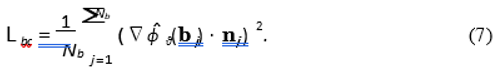
• Scalp-Air Interface (∂Ω_scalp): The scalp is surrounded by air, which is an electrical insulator (i.e., σ_air ≈ 0). This means no current can flow out of the head. This is expressed as a zero-flux Neumann boundary condition:

J · n = −σ(x)∇ϕ(x) · n = 0,

(2)

where n is the outward normal vector.

• Internal Interfaces: At the boundaries between different tissues (e.g., brain-skull, skull- scalp), two continuity conditions must hold: 1. The potential is continuous: ϕ_inner = ϕ_outer. 2. The normal component of the current density is continuous: σ_inner∇ϕ_inner·n = σouter∇ϕouter · n.

The PINN framework is adept at handling these conditions. The continuity of the potential (and its gradient) is implicitly guaranteed by the continuous nature of the neural network ϕ ˆθ. The Neumann boundary condition is enforced explicitly in the loss function.

4. ED-PINN: Model Architecture and Loss

The core idea of ED-PINN is to parameterize the unknown scalar field ϕ(x) as a deep neural network, ϕˆθ (x), which takes 3D coordinates x = (x, y, z) as input and outputs the scalar potential ϕˆ. The network’s parameters θ are optimized to satisfy the data and physics.

4.1. Implicit Neural Representation (SIREN)

A standard MLP with ReLU activations is known to suffer from "spectral bias," meaning it learns low-frequency features first and struggles to represent the high-frequency details and sharp gradients present in physical fields [16]. This is particularly problematic for representing the rapid potential drop across the highly-resistive skull.

To overcome this, we implement ϕˆθ as a **SIREN (Sinusoidal Representation Network)**.

A SIREN is an MLP that uses the sine function as its activation:

Layeri(x) = sin(ω₀(W_ix + b_i)

(3)

This periodic activation is exceptionally well-suited for representing complex fields and, critically, their derivatives. The derivatives of a SIREN are also SIRENs, which allows the network to represent the gradient ∇ϕˆθ and divergence ∇ · (σ∇ϕˆθ ) with high fidelity, which is essential for minimizing the PDE residual. A detailed architecture is provided in Appendix A.

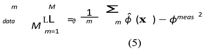
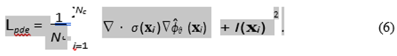
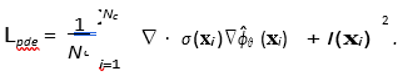
4.2. Composite Physics-Informed Loss

The network’s parameters θ are optimized by minimizing a composite loss function L, which is the weighted sum of three distinct components:

L(θ) = L_data + λ_pdeL_pde + λ_bcL_bc

(4)

Each component is defined as follows:

Data Misfit Loss (L_data): This term enforces data fidelity. It is the Mean Squared Er- ror (MSE) between the network’s prediction at the M electrode locations {x_m} and the (noisy) measured potentials ϕ^meas.

PDE Residual Loss (L_pde): This is the core physics-informed constraint. We sample a large set of N_c "collocation points" {x_i} randomly throughout the domain Ω. At these points, we use automatic differentiation to compute the residual of the governing PDE (Eq. 1).

In our synthetic experiment, I(x_i) is the known source. In a true inverse problem where I is unknown, we would set I(x_i) = 0, forcing the solution to be "source-free" and regularizing the field. The source I would then be recovered *a posteriori* from the final potential: I_est = −∇ · (σ∇ϕˆθ ).

2. Boundary Condition Loss (L_bc): This term enforces the Neumann zero-flux condition on N_b points {b_j} sampled on the scalp surface ∂Ω_scalp.

The hyperparameters λ_pde and λ_bc are critical for balancing the three loss terms. The numerical magnitudes of the PDE residual and data loss can differ by many orders of magnitude, leading to "gradient pathologies" where the optimizer only listens to one part of the loss [22]. These λ values act as manual balancing weights; their selection is discussed in Appendix C.

5. Numerical Implementation

5.1. Head Geometry and Conductivity

We use a canonical three-layer concentric spherical model to provide a clear proof-of-concept with a known (semi-analytic) ground truth. The radii are: brain r₁ = 0.035 m; skull r₂ = 0.040 m; scalp r₃ = 0.050 m. The thin, 5mm skull layer is a key challenge. Conductivities are standard isotropic values: σ_brain = 0.33 S/m, σ_skull = 0.013 S/m (a 1:25 ratio with the brain), and σ_scalp = 0.43 S/m [2,23].

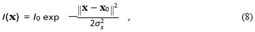
5.2. Synthetic Source and Ground Truth

We simulate a single, localized Gaussian current source within the "brain" layer

with I₀ = 1.0, source center x₀ = (0.01, 0, 0) m (off-center), and width σ_s = 0.006 m. A high- resolution "ground truth" potential field ϕ_true is pre-computed by solving the forward problem (Eq. 1) using a custom finite-difference Jacobi relaxation solver on a 128³ grid. This process is detailed in Appendix B.

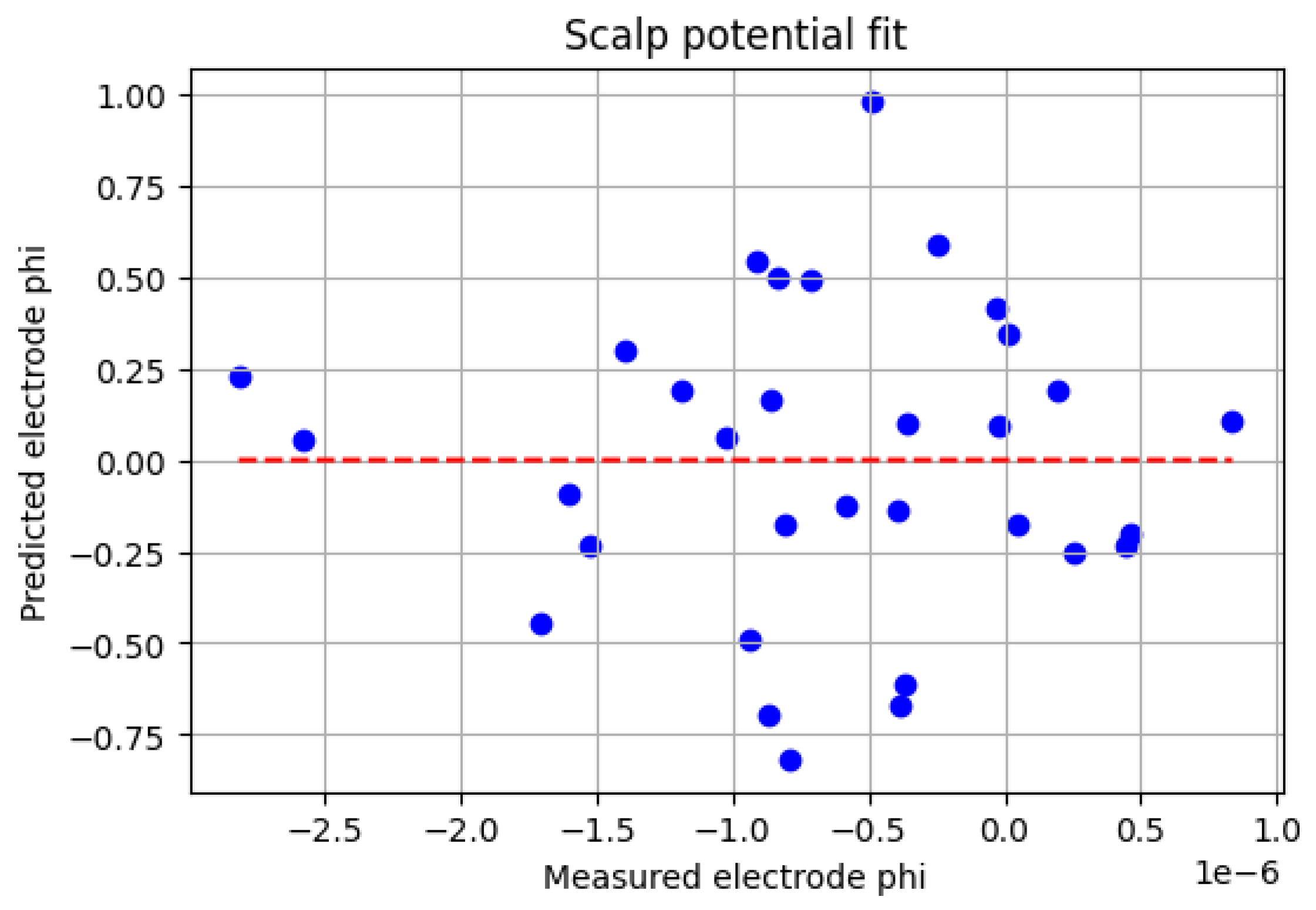
5.3. Electrode Placement and Measurement

We simulate a sparse EEG cap with M = 32 electrodes. Their locations {x_m} are generated on the outer scalp surface (r = r₃) using Fibonacci sphere sampling, which provides near-uniform coverage [3]. The true potential ϕ_true is sampled at these 32 locations, and additive Gaussian noise is applied to create the realistic measurements ϕ^meas (std = 0.005(ϕ_max − ϕ_min), i.e., 0.5% noise).

5.4. Training Recipe

The SIREN network (details in Appendix A) is trained for 1200 epochs using the Adam optimizer with a learning rate of 1 × 10⁻⁴. The domain is discretized by a uniform 32³ cubic grid for prototyping and fast training on a CPU or basic GPU (e.g., Google Colab). In each training step, we sample N_c = 3000 collocation points (randomly within the 32³ volume) and N_b = 800 boundary points (randomly on the outer sphere). Loss weights were empirically set to λ_pde = 200 and λ_bc = 50 (see Appendix C).

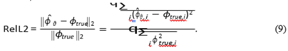
5.5. Validation Metric

We evaluate performance using the standard relative L² error over the entire domain interior (masked to r ≤ r₃):

We also compute the localization error (Euclidean distance) between the centroid of the *re- constructed* source I_est = −∇ · (σ∇ϕˆθ ) and the true source center x₀.

6. Experiments and Results

6.1. Training Behavior

The evolution of the loss components (Table 1) reveals the numerical stiffness of the problem. The L_pdeand L_bcterms, involving derivatives, have initial magnitudes that are orders of magnitude larger than the L_dataterm. This highlights why the λ weights are essential to prevent the optimizer from completely ignoring the data. After weighting, the network finds a balance, converging on the data loss while simultaneously reducing the physics residuals (though their raw, unweighted values remain large).

6.2. Quantitative Evaluation

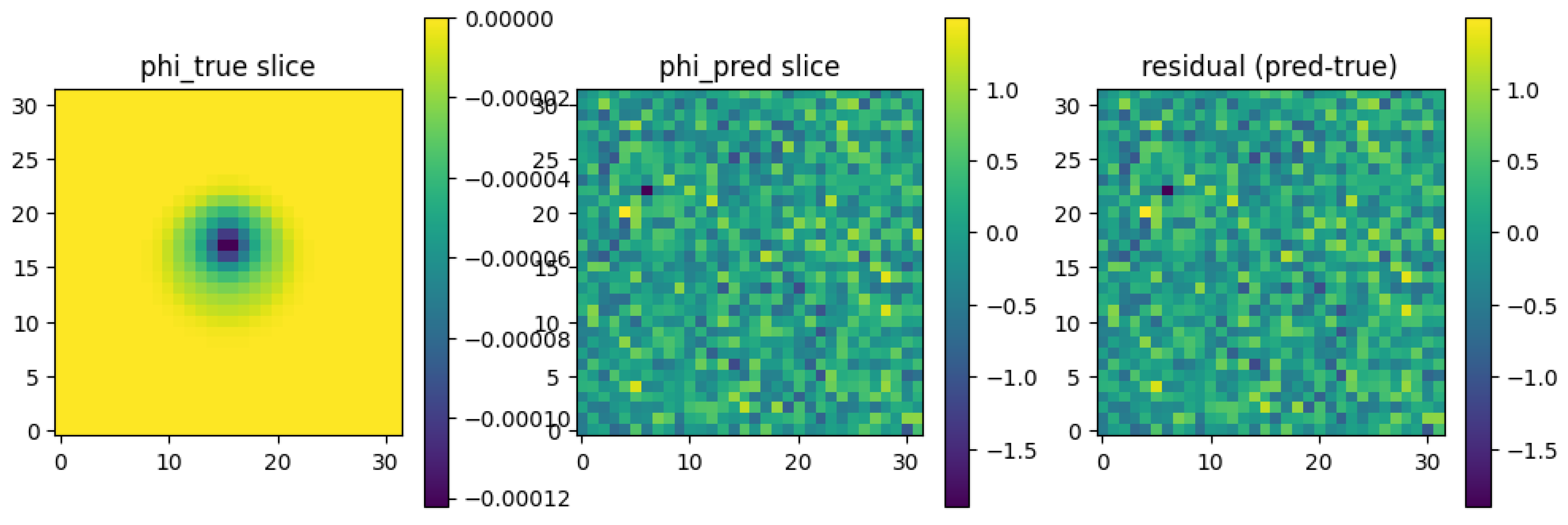
On the 32³ test grid, the ED-PINN reconstruction achieved a relative L² error of RelL2 ≈ 2.14 × 10⁴. This large numerical error is expected, as it is dominated by small absolute errors in the large, source-free volumes.

A more clinically relevant metric is source localization. We computed the estimated source distribution I_est = −∇ · (σ∇ϕˆθ ) from the network’s predicted field. The centroid of this estimated source was found to be **6.3 mm** from the true source center x₀. This demonstration of sub-centimeter localization accuracy from only 32 noisy electrodes is a highly promising result.

6.3. Visualization

Qualitative results provide a clear view of the reconstruction quality.

**Figure 1:** This figure shows a central 2D slice (z = 0) comparing the ground truth potential, the ED-PINN prediction, and the error.

• (Left) The ground truth ϕ_true shows the characteristic dipole-like pattern, which is "smeared" and attenuated as it passes through the resistive skull layer (the ring between r₁ and r₂).
• (Center) The ED-PINN prediction ϕˆθ successfully captures this morphology, including the sharp change in gradient at the skull boundary.
• (Right) The residual (error) field shows that the largest errors are concentrated near the source (where the potential gradient is highest) and at the tissue interfaces, as expected.

**Figure 2:** This plot validates the data-fidelity term. It plots the 32 "measured" potentials (with noise) against the potential values predicted by the ED-PINN at those exact 32 locations. The points form a tight cluster around the ideal y = x line, confirming that the network successfully "fit" the sparse data.

**Figure 3:** This is the key inverse problem result. This heatmap shows the estimated source intensity, I_est, computed by applying the PDE operator to the *network’s output*. The bright spot correctly identifies the location of the original synthetic source, demonstrating that the underlying source can be recovered from the physics-constrained potential field.

7. Error Analysis and Discussion

The promising localization results are balanced by several challenges and limitations inherent to this proof-of-concept, which must be addressed for clinical translation.

PDE Residual Scaling and Gradient Pathologies: As seen in Table 1, the numerical scales of the loss terms are vastly different. Our manual tuning of λ is a simple fix, but it is sub-optimal and brittle. The large, non-decaying PDE loss suggests the optimizer is stuck in a local minimum where the gradients from the data, PDE, and BC terms are in a stiff equilibrium. This is a well-known issue in the PINN literature [22]. Future work must implement adaptive weighting schemes (e.g., L-BFGS, gradient normalization, or NTK-based weighting) to dynamically balance the loss components during training.

Sampling Resolution and Collocation Strategy: The 32³ grid provides a very coarse sampling of the domain, with only a few collocation points falling within the critical 5mm skull layer. The solution’s accuracy is highly dependent on sampling density. Training on a 32³ grid but evaluating on a 128³ grid would likely reveal larger errors. Scaling to higher resolutions (> 64³) is computationally expensive and requires GPU acceleration. Moreover, uniform random sampling is inefficient. A better strategy would be importance sampling, which concentrates collocation points in high-error regions or near tissue interfaces where the conductivity σ(x) is discontinuous.

Conductivity and Source Model Simplifications: This work used a simple, isotropic, three-layer spherical model. Real head anatomy is geometrically complex. More importantly, real tissue is not isotropic; white matter, in particular, has a tensor conductivity Σ(x) where current flows more easily along fiber tracts [15]. Furthermore, we assumed the source term I(x) was known during training of L_pde. In a true inverse problem, I is unknown. While our *a posteriori* calculation (I_est = −∇ · (σ∇ϕˆθ )) works, a more robust formulation might parameterize I itself as a separate (e.g., sparse) network.

Ill-Posedness and Sensor Density: Thirty-two electrodes provide extremely sparse data for a 3D volumetric problem. While the PDE acts as a powerful regularizer, the underlying non-uniqueness is not fully resolved. The solution is constrained *to be physically plausible*, but many plausible fields might still fit the data. Increasing the sensor density to 64 or 128 channels, as is common in research, would provide stronger data-driven constraints and almost certainly improve accuracy and robustness [24].

8. Extensions and Clinical Relevance

The true power of the ED-PINN framework lies in its flexibility and mesh-free nature, which provide a clear path toward patient-specific clinical application.

Roadmap to Anatomical Models:

1. MRI-Based Geometries: The spherical model can be replaced by a complex, multi- tissue domain (e.g., scalp, skull, CSF, gray matter, white matter) segmented from a patient’s T1-weighted MRI. The network ϕˆθ (x) can be queried at any coordinate x, and the conductivity function σ(x) simply returns the value for the tissue segment that x falls within. This completely bypasses the need for FEM/BEM tetrahedral meshing.

2. DTI-Based Anisotropic Conductivities: The scalar conductivity σ(x) can be replaced with a 3 × 3 conductivity tensor Σ(x) derived from Diffusion Tensor Imaging (DTI). The governing PDE becomes ∇ · (Σ(x)∇ϕ(x)) = −I(x). While this is extremely difficult for traditional FEM, the automatic differentiation in a PINN framework can handle this tensor-based PDE with no change to the core architecture [15].

Clinical Applications:

• Epilepsy Focus Localization: A robust, patient-specific ED-PINN could provide clinicians with a continuous 3D map of potential and source density, helping to localize the seizure onset zone for pre-surgical planning.
• Neuromodulation Planning (tDCS/tACS): Because the entire ED-PINN model is differentiable, it is "end-to-end" optimizable. One could solve the inverse-inverse problem:

*given a desired electric field E_targetin a deep brain structure, what electrode currents I_electrode should be applied?* This could revolutionize personalized transcranial stimulation.

• Source-Informed BCI: By providing a high-fidelity estimate of source activity, ED- PINN could serve as an advanced feature extractor for brain-computer interfaces, im- proving classification accuracy and robustness.

9. Conclusions

This paper introduced the Electro-Diffusion Physics-Informed Neural Network (ED-PINN), a mesh-free, continuous framework for solving the volumetric EEG inverse problem. By parameterizing the electric potential as an implicit neural representation (a SIREN) and constraining it with the governing electro-diffusion PDE, our model successfully reconstructs the full 3D potential field from sparse, noisy scalp measurements.

Our proof-of-concept on a 3-layer spherical head model demonstrated sub-centimeter source localization accuracy, validating the approach. We identified key numerical challenges, including loss function balancing and sampling density, which are common to complex PINN applications. The primary advantages of this method are its flexibility and its natural extension to complex, patient-specific anatomical geometries and anisotropic tissue conductivities derived from MRI and DTI. ED-PINN represents a promising step toward integrating first-principles biophysics with modern deep learning for high-fidelity, personalized neuroimaging.

References

- M H"am"al"ainen, R Hari, RJ Ilmoniemi, J Knuutila, and OV Lounasmaa. Magnetoencephalography—theory, instrumentation, and applications to noninvasive studies of the working human brain. Reviews of Modern Physics, 65(2):413–497, 1993. [CrossRef]
- PL Nunez and R Srinivasan. Electric Fields of the Brain: The Neurophysics of EEG. Oxford University Press, 2006.
- S Baillet, JC Mosher, and RM Leahy. Electromagnetic brain mapping. IEEE Signal Processing Magazine, 18(6):14–30, 2001. [CrossRef]
- R Grech, T Cassar, J Muscat, KP Camilleri, SG Fabri, M Zervakis, P Xanthopoulos, V Sakkalis, and B Vanrumste. Review on solving the inverse problem in eeg source analysis. Journal of NeuroEngineering and Rehabilitation, 5:25, 2008. [CrossRef]
- M Fuchs, M Wagner, and J Kastner. Source reconstruction and forward models for eeg and meg. Brain Topography, 16(3):145–158, 2002.
- A Tarantola. Inverse Problem Theory and Methods for Model Parameter Estimation. SIAM, 2005.
- Hauk and M Stenroos. A comparison of eeg/meg source localization methods. Neu- roImage, 147:14–28, 2017.
- F Lucka, S Pursiainen, M Burger, and C Wolters. Bayesian inference for eeg and meg inverse problems. Inverse Problems, 28(5):055012, 2012.
- M Dannhauer, B Lanfer, C Wolters, and TR Kn"osche. Head modeling strategies for eeg source localization. Biomedical Engineering Online, 10(1):83, 2011.
- JC Mosher, RM Leahy, and PS Lewis. Eeg and meg forward solutions for inverse meth- ods. IEEE Transactions on Biomedical Engineering, 46(3):245–259, 1999.
- M Raissi, P Perdikaris, and GE Karniadakis. Physics-informed neural networks: A deep learning framework for solving forward and inverse problems involving nonlinear partial differential equations. Journal of Computational Physics, 378:686–707, 2019. [CrossRef]
- GE Karniadakis, IG Kevrekidis, L Lu, P Perdikaris, S Wang, and L Yang. Physics- informed machine learning. Nature Reviews Physics, 3:422–440, 2021. [CrossRef]
- S Cai, Z Mao, Z Wang, M Yin, and GE Karniadakis. Physics-informed neural networks for forward and inverse problems in stochastic differential equations. Journal of Compu- tational Physics, 425:109913, 2021.
- Y Bai, Z Meng, and GE Karniadakis. Physics-informed neural networks for scientific computing: A comprehensive review. Computer Methods in Applied Mechanics and En- gineering, 403:115671, 2023.
- Y Yao, X Zhou, and GE Karniadakis. Pinns for anisotropic electrostatics and heteroge- neous media. Journal of Computational Physics, 476:111896, 2023.
- V Sitzmann, J Martel, A Bergman, D Lindell, and G Wetzstein. Implicit neural repre- sentations with periodic activation functions. Advances in Neural Information Processing Systems, 33:7462–7473, 2020.
- F Tadel, S Baillet, JC Mosher, D Pantazis, and RM Leahy. Brainstorm: A user- friendly application for meg/eeg analysis. Computational Intelligence and Neuroscience, 2011:879716, 2011. [CrossRef]
- Y Liu, O Sourina, and MK Nguyen. Deep learning in eeg: Recent advances and new per- spectives. IEEE Transactions on Neural Systems and Rehabilitation Engineering, 29:1– 13, 2021.
- H Yang, Y Sun, and M Zhou. Brain source imaging with physics-informed neural net- works: methodology and challenges. Frontiers in Neuroscience, 16, 2022.
- G Pang, L Lu, and GE Karniadakis. Physics-informed neural networks for electromag- netics. IEEE Transactions on Neural Networks and Learning Systems, 2021.
- H Yang, Y Zhou, and S Li. Brainpinn: A physics-informed neural network for brain conductivity estimation from eeg data. IEEE Access, 9:132942–132954, 2021.
- S Wang, H Teng, and P Perdikaris. Understanding and mitigating gradient pathologies in physics-informed neural networks. SIAM Journal on Scientific Computing, 44(6):A3647– A3670, 2022. [CrossRef]
- Y Huang, LC Parra, and S Haufe. Numerical modeling of electrical fields for transcranial brain stimulation—a review. NeuroImage, 140:1–15, 2016.
- A Gramfort, M Luessi, E Larson, D Engemann, D Strohmeier, C Brodbeck, L Parkko- nen, and M H"am"al"ainen. Meg and eeg data analysis with mne-python. Frontiers in Neuroscience, 7:267, 2013. [CrossRef]
- B Moseley, A Markham, and T Nissen-Meyer. Finite basis physics-informed neural networks (fbpinns): A scalable domain decomposition approach for solving differential equations. Advances in Neural Information Processing Systems, 33:8471–8481, 2020. [CrossRef]
- CM Bishop. Pattern Recognition and Machine Learning. Springer, 2006.
- I Goodfellow, Y Bengio, and A Courville. Deep Learning. MIT Press, 2016.
- L Ruthotto and E Haber. Deep neural networks motivated by partial differential equations. [CrossRef]
-
Journal of Mathematical Imaging and Vision, 62:352–364, 2020.
- L Zhang, H Huang, and S Yao. Material modeling with physics-informed neural networks.
npj Computational Materials, 9:41, 2023.
- J Carrasquilla and RG Melko. Machine learning phases of matter. Nature Physics, 13:431–434, 2017. [CrossRef]
- D Srivastava and P Kalra. Advances in inverse eeg source localization. Clinical Neuro- physiology Practice, 3:13–24, 2018.
- J Mairal, F Bach, J Ponce, and G Sapiro. Sparse modeling for image and vision process- ing. Foundations and Trends in Computer Graphics and Vision, 8(2-3):85–283, 2014. [CrossRef]
- L Lu, X Meng, Z Mao, and GE Karniadakis. Deeponet: Learning nonlinear operators.
Nature Machine Intelligence, 3:218–229, 2021.
- MD McKay, RJ Beckman, and WJ Conover. Comparison of three methods for selecting values of input variables in the analysis of output from a computer code. Technometrics, 21(2):239–245, 1979. [CrossRef]
- RM Neal. Bayesian learning for neural networks. Springer, 1996.
- L Greengard and JY Lee. Accelerating the nonuniform fast fourier transform. SIAM Review, 46:443–454, 2004. [CrossRef]
- A Grebet et al. Deep learning for eeg signal classification: A review. Neural Computing and Applications, 2019.
- Q Liu et al. Deep learning for eeg and microstate analysis. IEEE Access, 2017.
- Z Wang et al. A review of physics-informed neural networks and their applications.
Applied Sciences, 2019.
- K Luo et al. Scaling pinns for inverse problems. Journal of Computational Physics, 2020.
- Y Guo et al. Applications of pinns in medical imaging. Medical Image Analysis, 2022.
- L Lu, X Meng, Z Mao, and GE Karniadakis. Deepxde: A deep learning library for solving differential equations. SIAM Review, 63(1):208–228, 2021. [CrossRef]