
Submitted:
25 January 2026
Posted:
26 January 2026
You are already at the latest version
Abstract
Ground-level building damage assessment captures critical structural details that remain invisible in satellite imagery, yet this perspective remains severely underexplored in current research. We address this gap by introducing the first war damage dataset for ground-level building segmentation, comprising high-resolution side-view images of war-affected Ukrainian buildings with pixel-wise annotations across six semantic classes: Other, Building, Roof, Damage, Damaged Roof, and Broken Window. To preserve original image resolution while enabling efficient deep learning, we employ a patch-based strategy that divides each image into fixed-size regions, generating thousands of training samples from the original dataset. We propose an embedding-enhanced U-Net framework that enriches each patch with global ConvNeXt-Large embeddings and positional encodings to provide scene-level context and spatial awareness. We systematically evaluate six encoder architectures(ResNet-50, SwinV2-Large, ConvNeXt-Large, YOLO11x-seg, DINOv2, and SegFormer-b5) across 48 configurations, testing both simplified three-class and complex six-class segmentation tasks with and without embedding integration and Felzenszwalb superpixel post-processing. Results demonstrate substantial performance gains from embedding integration: ResNet-50 achieved +7.81 pp IoU improvement, reaching 0.7743 IoU and 0.8982 F1-score for three-class segmentation, while DINOv2 attained optimal six-class performance with 0.4711 IoU and 0.7462 F1-score, representing a +4.65 pp IoU gain.
Keywords:
semantic segmentation
; building damage
; ground-level imagery
; U-Net
; embeddings
; ResNet
; SwinV2
; ConvNeXt
; DINOv2
; Felzenszwalb superpixels
1. Introduction
Nowadays, cities are growing fast, and the consequences of damage from war, earthquakes, and other disasters are becoming more serious and frequent. As a result, it is crucial to inspect the condition of buildings promptly after such events. A fast and accurate assessment enables emergency services to respond more effectively, plan repairs, and utilize resources more efficiently.
Manual inspections are generally accurate, but they require a significant amount of time, can be subjective, and pose risks in unsafe areas. Automated systems that use image analysis, especially deep learning methods, provide a faster and more consistent way to assess damage. Until now, most such systems have used images from satellites or drones to check large areas. However, many important types of building damage, such as cracks in walls, broken windows, or parts of the building falling, can only be seen clearly from ground level. For this reason, systems that analyze ground-level photos are crucial for understanding the actual situation in cities, especially in areas where buildings are partially obscured or difficult to see from above.
Most current research on building damage segmentation focuses on the use of satellite imagery. Many of such systems perform multiclass segmentation where each pixel is labeled according to the severity of the structural damage [1,2]. Some approaches combine pre-disaster and post-disaster images, along with auxiliary geospatial data, to improve segmentation results [3]. Another study introduces a damage segmentation system designed explicitly for war-affected areas in Syria [4]. A notable event in this field is the xView2 challenge [5], which uses the xBD dataset [6] and aims to identify buildings and rate the damage amount. This dataset contains around 850.000 annotated buildings spanning 45,000 square kilometers of satellite imagery and serves as a benchmark for damage classification from space.
There are also researches based on aerial imagery captured by drones. For example, [7] presents a segmentation dataset that includes various damage classes for buildings, along with road, vegetation, and other contextual features. This study also evaluates a set of segmentation models. Similarly, [8] compares different segmentation methods using post-earthquake aerial images to assess how well they perform in real-world disaster conditions.
However, the task of building damage assessment from ground-level imagery remains significantly underexplored compared to aerial approaches. Ground-level facade analysis has primarily focused on undamaged buildings, with research addressing various architectural elements and structural patterns.
Several studies have developed segmentation systems for building facades using street-view imagery. [9] introduced a dataset of 1057 annotated images from 104 countries, focusing on irregular and non-regular facades with six classes, including background, plant, wall, window, door, and fence. The study evaluated multiple CNN architectures including U-Net [10], DeepLabv3+[11], SegNeXt [12], HRNet [13], and PSPNet [14] on images resized to 512×512 pixels. [15] collected 997 high-resolution side-view building images from a single city in England, implementing a two-stage approach where one U-Net model segments large objects like walls and roofs, while another focuses on smaller elements such as windows, doors, and chimneys after object detection-based cropping. [16] presented a street-view dataset of 500 images with five facade classes, combining DeepLabV3 segmentation with R-CNN-based [17] detection to improve boundary accuracy through quadrilateral refinement of detected objects. Recent advances in transformer-based architectures have also been applied to facade segmentation. [18] developed a dataset of 602 high-resolution street-view images, employing Vision Transformer [19] architectures including Segmenter [20] with ViT-B/16 and ViT-L/16 backbones. The study incorporated line detection methods to enhance segmentation boundaries and edge quality. [21] applied Fully Convolutional Networks based on VGG-16 [22] to two facade datasets, the first with 104 images and the second with 60 images, combining segmentation with object detection to improve accuracy for smaller architectural elements. The application of deep learning to structural damage assessment from ground-level perspectives has received limited attention. [23] addressed earthquake damage detection using 856 images cropped to 800×800 pixels, implementing a modified YOLO v5 [24] architecture to detect four damage classes: debris, collapse, spalling, and cracks. [25] tackled facade damage segmentation using 1761 infrared and visible images, identifying four damage types, including moisture, efflorescence, cracks, and cavities. This work combined thermal and visible imagery through GAN-based fusion before applying YOLO-based segmentation architectures. [26] focused specifically on crack segmentation in structural elements, developing a modified U-Net encoder-decoder architecture that reduced model parameters while maintaining segmentation accuracy on images resized to 256×256 pixels.
To the best of our knowledge, there are no publicly available datasets annotated for pixel-wise segmentation of building damage in ground-level images. There are also no models or systems in the literature that have been evaluated for this specific task. This gap motivates our work: we introduce a new annotated dataset of ground-level damage images and provide a comparative evaluation of several segmentation architectures specifically tailored for this setting.
In recent years, deep learning has significantly improved the performance of semantic segmentation tasks. Convolutional neural networks became the foundation of many image understanding systems. One of the most well-known architectures in this field is the U-Net, which was originally designed for biomedical image segmentation. Its encoder-decoder structure with skip connections helps the network preserve spatial detail while learning high-level features. U-Net has since been adapted for a wide range of tasks, including urban scene segmentation.
To further improve feature extraction, many U-Net-based systems use powerful pretrained encoders. They include ResNet [27], which, with its residual blocks, provides deep representations that help capture complex patterns. SwinV2 [28] and ConvNeXt [29] are examples of more recent architectures that combine CNN and transformer principles, enabling better long-range feature modeling and global context awareness. Transformer-based architectures, such as SegFormer [30], have also garnered attention for their efficient segmentation pipelines and strong performance on various benchmarks. Meanwhile, YOLO 11x-seg [31] extends real-time object detection models into the segmentation domain by adding spatial decoding layers. DINOv2 [32], a self-supervised transformer-based model, provides strong general-purpose visual representations and has demonstrated competitive results in dense prediction tasks. Together, these architectures represent different design philosophies. CNNs, transformers, and hybrid models, all of which can be evaluated to determine which works best for the unique challenges of ground-level building damage segmentation.
Beyond the backbones directly tested in this work, a wide range of other encoder architectures exist. Classic CNN-based encoders, such as VGG or DenseNet [33], have historically been popular for their simplicity and feature reuse but are now often surpassed by more advanced residual and transformer-based designs. Hybrid models like EfficientNet [34] aim for optimized scaling of depth, width, and resolution, offering strong performance with relatively fewer parameters. Pure transformer backbones such as ViT and DeiT [35] demonstrate powerful global context reasoning, though their high data and compute requirements often limit their application in domains with smaller datasets. More recent approaches include foundation models such as CLIP [36], which align vision and language representations to enable zero-shot transfer, and SAM (Segment Anything Model)[37], which generalizes segmentation through prompt-based interaction.
In addition to alternative backbones, many modifications of the U-Net itself have been proposed. Variants such as Attention U-Net [38] incorporate attention mechanisms to better focus on relevant spatial regions, while U-Net++[39] introduces nested and dense skip connections to enhance feature fusion between encoder and decoder. Other adaptations include ResUNet [40], which integrates residual connections for deeper representation learning, and TransUNet [41], which combines the U-Net’s decoder design with transformer-based encoders to capture both local and global dependencies. Lightweight versions, such as Mobile U-Net [42], have been developed for real-time or resource-limited applications. While these architectures extend the U-Net’s applicability and often improve task-specific performance, in this work, we employed the baseline U-Net framework to provide a straightforward and comparable foundation for testing different encoder choices under the same segmentation pipeline.
Ground-level images present several challenges that make the task of damage segmentation more difficult than aerial or satellite imagery. Firstly, available datasets for this type of data are usually small and contain limited annotations, making it hard to train large models without overfitting. In many cases, collecting labeled data at ground level is time-consuming and expensive, especially in post-disaster environments. Secondly, these images often contain partial occlusions from trees, vehicles, fences, or other urban elements. Such visual clutter can hide key parts of the building or distort the appearance of damaged areas. Thirdly, lighting conditions vary greatl - shadows, reflections, weather, and time of day can significantly change the visibility and contrast in the images. Camera angles are also inconsistent, as ground-level photos are taken from different heights and perspectives, which may affect how certain structures appear. Finally, there is a significant class imbalance in the data. Common categories such as background and undamaged building parts dominate the dataset, while important damage types like “Broken Window” or “Debris” appear far less often. This imbalance may lead models to perform poorly on rare but critical classes.
To the best of our knowledge, there is currently no standardized dataset or benchmark designed specifically for pixel-wise segmentation of building damage in ground-level images. This lack of annotated data for ground-level damage segmentation has made it difficult to compare models fairly or to develop methods that are optimized for real-world urban environments. At the same time, there is no comprehensive study that evaluates how modern segmentation architectures—particularly those using advanced encoder backbones or embedding strategies - perform in such types of data.
Our study aims to address this gap by creating a custom dataset of manually labeled ground-level images and by testing several encoder architectures’ training ability on this task. This makes it possible to analyze the strengths and limitations of different methods and to set a foundation for future research in this area.
This paper presents a complete pipeline for semantic segmentation of building damage from ground-level images. The main contributions of the study are:
- We introduce a custom-labeled dataset of 290 urban images taken from a ground-level perspective. Each image is manually annotated with six semantic classes related to structural damage and building context.
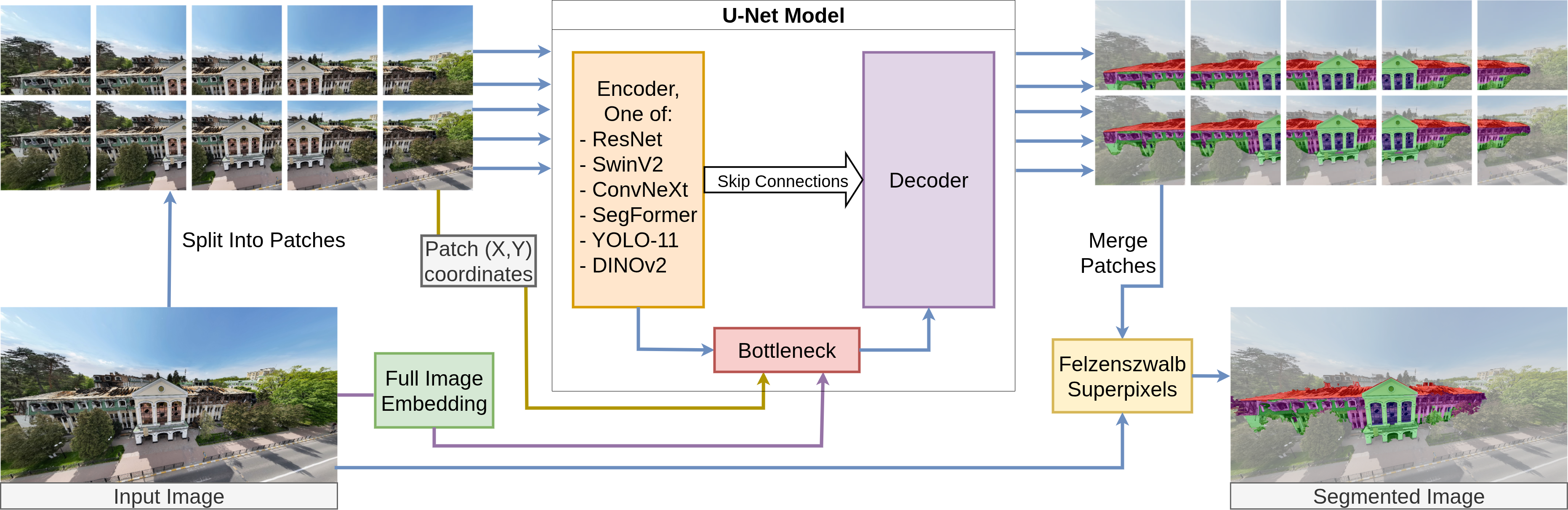
- We design a patch-based segmentation approach using a modified U-Net architecture. Each image is divided into fixed-size patches, which are enriched with global image embeddings generated by a pretrained ConvNeXt-Large model. These embeddings provide context about the entire scene, helping the model better understand each local region.
- To give the model awareness of spatial layout, we include positional embeddings that encode the patch’s location within the image.
- We apply Felzenszwalb’s [43] superpixel-based post-processing to refine the model’s output and reduce visual noise in the segmentation maps.
- We perform a comparative evaluation of five different encoder backbones - ResNet-50. SwinV2-Large, ConvNeXt-Large, YOLO 11x-seg, and DINOv2 - as well as a modified version of SegFormer-b5, providing insights into how these architectures perform in the context of ground-level building damage segmentation.
These contributions help build a foundation for more robust and practical deep learning systems that can be deployed in urban disaster response and smart infrastructure damage assessment.
2. Materials and Methods
2.1. Dataset Collection and Annotation
In this study, we introduce a new dataset designed for the semantic segmentation of building damage in Ukrainian urban environments. The dataset consists of 290 ground-level images collected from open sources, including news websites, public Telegram channels, social media posts, and other freely accessible online platforms. The photos were taken under various conditions, including different lighting, angles, and weather situations, which provides important visual diversity for robust model training. All images were manually annotated using the Computer Vision Annotation Tool (CVAT) [44], with each pixel labeled according to one of six semantic classes:
- Other - background and non-structural objects (gray)
- Building - general building structures (green)
- Roof - undamaged roof sections (orange)
- Damage - damaged parts of buildings, excluding roofs and windows (purple)
- Damaged Roof - visibly destroyed or collapsed roof areas (red)
- Broken Window - shattered or missing windows (blue)
The segmentation masks were saved in a single XML file, which includes polygon coordinates and bounding boxes for all 290 images. Each image is linked to its annotations via unique identifiers inside the XML structure. While the dataset provides high-quality polygon annotations, some inconsistencies and minor errors may be present. In certain cases, boundaries may be drawn too broadly, particularly when foreground objects overlap with buildings. For example, if a tree partially covers a facade, the annotation sometimes includes the tree region that lies over the building instead of masking only the building itself. Such cases introduce slight label noise and may affect segmentation accuracy for fine details. For better understanding, Figure 1 shows examples of annotated images, with the corresponding class colors overlayed. These visualizations demonstrate the typical scene complexity and the diversity of damage patterns captured in the dataset.
The dataset exhibits a strong class imbalance, which reflects the real-world prevalence of certain features over others. The class distribution is shown in Table 1. As can be seen, the majority of labeled pixels belong to the class Other (66.10%) and Building (19.42%), while more critical damage-related classes such as Broken Window and Damaged Roof are underrepresented (2.66% and 1.92% respectively).
2.2. Patch-Based Representation and Embedding Integration
To improve segmentation performance under high class imbalance and preserve fine local details, we introduce a patch-based training strategy that forms the foundation of our pipeline. Instead of training directly on full-resolution images, each original image is divided into fixed-size square patches using a sliding window approach with a defined stride. This allows the model to focus on localized regions while maintaining spatial coherence across the image.
A patch is defined as a smaller, square region cropped from the full image. The division is performed by sliding a window of fixed size (e.g., 224×224, 384×384, or 640×640 pixels) across the image using a preset stride. For each extracted patch, the corresponding segmentation mask is also cropped to match the spatial region of the patch. This patching strategy significantly increases the number of training samples and improves learning stability. To ensure consistency in patch shape and facilitate batch processing during training, all patches must be of a fixed and uniform size. However, image dimensions often vary and are not always divisible by the selected patch size or stride. To address this, we apply a resizing operation before patching, scaling the entire image to a fixed resolution that guarantees complete and uniform coverage. This means that if either the height or width of an image would result in an incomplete final patch (e.g., a partial region smaller than the target size), the image is rescaled such that both dimensions become divisible by the stride or the patch size. This resizing step ensures that every extracted patch is of exactly the required dimensions, preventing the need for padding or discarding remainder regions. As a result, the training set contains only complete, valid patches that conform to the model’s input expectations.
In addition to the raw image patch, we provide the segmentation model with two auxiliary embeddings that enrich the input representation:
- Global image embedding: Each input image (resized to 384×384 before the embedding extraction) is also represented by a global embedding extracted with a pretrained ConvNeXt-Large model. This results in a fixed 1536-dimensional vector that encodes the overall scene context. While the segmentation network processes local patches independently, the global embedding provides complementary information about the entire image layout. This helps the model distinguish between visually similar local regions by grounding them in the broader scene structure, for example, recognizing that a small texture patch belongs to a building facade rather than a background object.
- Positional embedding: Each patch is assigned a 2D coordinate vector that represents its relative position (x,y) within the original image grid. This positional encoding enables the model to preserve spatial relationships and enhance the consistency of predictions across adjacent patches. The positional vectors are normalized and have a fixed length of 2, capturing the horizontal and vertical offset of the patch’s top-left corner.
Thus, the final input to the segmentation model is a triplet:
- The image patch and its corresponding segmentation mask;
- The global context embedding;
- The positional embedding.
The design in Figure 2 illustrates the end-to-end flow of how patches are extracted, embeddings are computed, and the combined representation forms one item in the patch dataset. As shown, each image is first resized (if necessary) and then split into fixed-size patches. Global image embeddings are computed once per image, while positional embeddings are computed per patch. These are all fused before entering the model. This input structure enables the network to maintain both local precision (via high-resolution patches and masks) and global spatial awareness (via embeddings).
2.3. Dataset Preparation and Splitting
We constructed six separate patch-based datasets by combining two class schemes:
- Six classes - Other, Building, Roof, Damage, Damaged Roof, Broken Window;
- Three classes - Other, Building, Damage. Roof is merged into Building, and Broken Window and Damaged Roof are merged into Damage.
As classes Roof, Broken Window, and Damaged Roof are severely underrepresented in the data, in the second dataset, we merge them into semantically similar classes to make our metrics more robust. Each class schema has three patch configurations (224×224, 384×384, and 640×640 pixels), depending on the encoder for the global embeddings. For each configuration, we used a sliding window to extract square patches with a fixed stride, ensuring coverage of the entire image. When image dimensions were not divisible by the stride, we applied resizing to guarantee that all extracted patches were uniform in size (as described in Section 2.2).
The original dataset of 290 labeled images was split into 246 training and 44 validation images using an 85:15 ratio. Patches and corresponding segmentation masks were then extracted from each subset. The datasets differ by patch size and stride, selected based on the input resolution of the target segmentation models (e.g., ResNet-50, SwinV2-Large, ConvNeXt-Large). Table 2 summarizes the configuration and size of each dataset variant.
To improve model generalization and mitigate overfitting, we applied a set of image-mask paired augmentations to all training patches:
- Random Resized Crop(size = original patch size; scale = (0.6, 0.8)) - Randomly crops a part of the input image and resizes it back to the original patch size. The scale parameter defines the relative area of the crop compared to the original image, here randomly chosen between 60% and 80%. This helps the model learn robustness to partial views of objects;
- Horizontal Flip (probability(p) = 0.5) - Flips the image horizontally with probability p. A value of 0.5 means that half of the images are mirrored, improving invariance to left-right orientation;
- HSV shifts (hue shift limit=20, saturation shift limit=30, value shift limit=20, p=0.3) - Randomly alters the hue, saturation, and brightness of the image. The parameters define the maximum allowed shift: hue can change by ±20 degrees, saturation by ±30 units, and brightness by ±20 units. With p = 0.3, this augmentation is applied to 30% of the images;
- Random Brightness Contrast (brightness limit=0.15, contrast limit=0.15, p=0.4) - Randomly adjusts the brightness and contrast of the image. The brightness and contrast are changed by up to ±15% of the original values. The probability p = 0.4 means this is applied to 40% of the images;
- Gaussian Noise (std range = (0.1, 0.2), p=0.4) - Adds Gaussian-distributed noise to the image, with the standard deviation randomly sampled between 0.1 and 0.2. This encourages the model to be more robust to noisy inputs. Applied with probability p = 0.4;
- Elastic Transform (alpha=20, sigma=60, p=0.4) - Applies random elastic deformations to the image, simulating realistic spatial distortions. The parameter alpha controls the intensity of the displacement, while sigma determines the smoothness of the deformation field. With p = 0.4, this is applied to 40% of the images.
All augmentations were applied on-the-fly during training using consistent random seeds and synchronized transformations for both the image and its mask to preserve spatial alignment.
To reduce training time and ensure consistency across experiments, all six patch datasets were precomputed and cached. Each dataset was generated once and then saved to Google Drive in a structured format, with separate folders for training and validation patches, masks, and their corresponding embedding vectors. At the beginning of each training session, the selected dataset is downloaded into local storage, allowing for fast access during model execution. This approach eliminates the need to recreate patches or recompute embeddings during training, making the data pipeline both reproducible and efficient. During training, only data augmentations are applied on-the-fly to the locally stored patches, while the patch structure and label integrity remain unchanged. This design significantly reduces preprocessing overhead and enables rapid experimentation with different model architectures and hyperparameter settings.
2.4. Overview of Modified U-Net
The base architecture adopted in this study is the classical U-Net architecture, which we modify to support patch-based processing and auxiliary embeddings. U-Net remains a widely used structure for semantic segmentation due to its effective combination of spatial precision and contextual representation. It is particularly well-suited for dense prediction tasks, such as pixel-wise damage detection in visually complex and partially occluded urban scenes. U-Net consists of two symmetrical parts: an encoder path, which reduces the spatial resolution and extracts high-level features, and a decoder path, which progressively restores spatial detail to construct a full-resolution segmentation mask. These parts are connected by a central bottleneck layer that aggregates the most compressed representation of the input. A defining feature of U-Net is the use of skip connections between corresponding levels of the encoder and decoder. These connections allow detailed spatial features from earlier stages to directly inform later decoding steps, improving localization accuracy.
In our implementation, the U-Net architecture is modified to integrate patch-based inputs and auxiliary embeddings. Each patch is first processed by an encoder backbone. The encoder output is then concatenated with two additional vectors: a global image embedding, extracted from the full image using a pretrained ConvNeXt-Large model, and a positional embedding, which encodes the (x, y) location of the patch within the original image. This combined representation is passed into the bottleneck. In the decoder path, we replace transposed convolutions with bilinear interpolation followed by standard convolution, while maintaining skip connections to corresponding decoder blocks.
A high-level overview of this architecture is shown in Figure 3. Detailed descriptions of the encoder backbones, bottleneck design, and decoder blocks are provided in Section 2.5 and Section 2.6.
2.5. Encoder Variants
To evaluate the impact of different backbone designs on segmentation quality, we incorporated five distinct encoder architectures into our modified U-Net framework: ResNet-50. SwinV2 Large, ConvNeXt Large, YOLO 11x-seg, and DINOv2. All models were initialized with pretrained weights and subsequently fine-tuned on our dataset. Each encoder was paired with a specific patch dataset, selected to align with its optimal input resolution. The patch sizes and strides were defined during dataset preparation (see Table 2) and reused for all downstream training. The output feature maps from intermediate encoder stages were used as skip connections in the decoder path, and their selection varied depending on the internal structure of each encoder model. A summary of the encoders, their parameter counts, chosen patch sets, and selected skip connection layers is presented in Table 3.
ResNet-50 is a convolutional architecture composed of an initial convolutional stem (conv1), followed by four sequential residual stages (layer1 to layer4). Each stage applies a series of residual blocks that progressively reduce spatial resolution while increasing semantic depth. The residual connections within each block facilitate gradient flow, enabling stable training of deep networks. In our system, ResNet-50 was used as the encoder with an input patch size of 224×224 and a stride of 180. consistent with its canonical design. Intermediate feature maps were extracted from conv1, layer1, layer2, and layer3 for skip connections, supporting multi-scale fusion in the decoder. The output of layer4 served as the encoder’s final representation and was forwarded to the bottleneck.
SwinV2 Large is a hierarchical Vision Transformer that applies self-attention within shifted, non-overlapping windows, achieving linear complexity with respect to image resolution. The architecture consists of four stages, each reducing spatial resolution while expanding feature dimensionality, analogous to the pyramidal design in convolutional encoders. For our experiments, SwinV2 was fine-tuned using a patch dataset with a resolution of 384×384 and a stride of 256, matching the model’s native input size. Feature maps were extracted from the outputs of stages 1, 2, and 3 for use in skip connections. The output of stage 4 served as the final encoder representation and was passed to the bottleneck. To reduce overfitting, all dropout layers were set to 0.5. Additionally, a few early layers of the encoder were kept frozen during fine-tuning.
ConvNeXt Large is a convolutional backbone redesigned for competitive performance with vision transformers. It incorporates depthwise separable convolutions, large kernel sizes (7×7), and LayerNorm in place of BatchNorm, while preserving a hierarchical four-stage architecture with progressive downsampling. The model was fine-tuned on 640×640 image patches with a stride of 160, in line with its design for high-resolution inputs. Feature maps were extracted from the downsampling outputs at the end of stages 1 through 3 for skip connections. The output of stage 4 was used as the encoder representation for the bottleneck. To improve regularization, all dropout layers were configured with a dropout rate of 0.6.
The encoder derived from the YOLO 11x-seg model leverages a deep stack of convolutional, CSP, and transformer blocks originally designed for efficient real-time object detection. In our adaptation for segmentation, the model’s intermediate layers were repurposed to serve as multiscale feature extractors. Specifically, the outputs from layers 1, 3, and 5 were used as skip connections to the decoder, providing hierarchical spatial context. The output of layer 7, which captures the deepest and most abstract features, was passed to the bottleneck block and fused with global and positional embeddings. The encoder was trained using a 640×640 patch dataset with a stride of 160. ensuring alignment with the input expectations of the backbone.
Another encoder utilizes the ViT-L/14 backbone from DINOv2, a self-supervised vision transformer trained via self-distillation without labeled data. It was selected for its capacity to learn semantically rich representations from the global context. Training was performed on 640×640 patches, which were resized to 518×518 during augmentation to meet the input constraints of the model. Outputs from transformer blocks 1, 7, and 12 were used as skip connections to provide multiscale features with controlled memory consumption. The output of block 20 served as the encoder output and was passed to the bottleneck.
2.6. Decoder and Fusion
The central bottleneck block in our architecture plays a critical integrative role by combining three distinct streams of information: high-level feature maps from the deepest encoder layer, a global image embedding, and a positional embedding representing the (x, y) coordinates of the current patch within the original image. This design extends the classical U-Net bottleneck with a semantically enriched representation that injects global and positional context directly into the decoding pipeline. The global image embedding is obtained by passing the full-resolution input image through a pretrained ConvNeXt-Large network and extracting the final 1536-dimensional vector. In parallel, each patch’s relative location, normalized in the range [0, 1] is encoded as a 2-dimensional positional vector. Before fusion, both embeddings are projected through dedicated linear layers to reduce dimensionality and enhance compatibility with the spatial tensor structure of the encoder output. These projections are then broadcast to match the spatial dimensions of the encoder’s final feature map and concatenated along the channel axis. The resulting tensor, rich in semantic and positional information, is processed by a convolutional bottleneck block, which serves as the starting point for the decoding path.
The decoder follows the standard U-shaped design and performs progressive spatial upsampling through four stages of decoding. At each stage, bilinear interpolation is used in place of transposed convolutions to restore spatial resolution. This choice significantly reduces the number of learnable parameters and helps avoid the checkerboard artifacts that often arise from learned upsampling filters. Following interpolation, feature maps are concatenated with the corresponding skip connections from the encoder, preserving low-level details and enhancing spatial precision. Each concatenated tensor is processed by a dedicated decoder block comprising a convolution, batch normalization, activation function(for most architectures, we used GELU), and dropout layers, progressively narrowing the channel dimensions and refining segmentation boundaries. The final stage restores the resolution to the original patch size and outputs the semantic segmentation mask through a 1×1 convolutional layer projecting to the target number of classes.
2.7. Overview of Modified SegFormer
In addition to the U-Net-based models, we implemented a modified version of the transformer-based SegFormer-B5 architecture adapted to the same segmentation framework. The SegFormer backbone follows a hierarchical vision transformer design, which internally computes multiscale representations via attention across spatially partitioned windows. For our setup, it was used as a feature encoder that outputs a single high-level feature tensor. SegFormer-B5 was applied to the same patch-level inputs as the other models, 640×640 patches with a stride of 160, to ensure consistency across encoder variants. The encoder output, a high-dimensional tensor containing the final semantic features, was passed into a bottleneck block along with two auxiliary embeddings: a global context vector obtained from a ConvNeXt-Large model and a normalized positional embedding encoding the spatial coordinates of the patch. These embeddings were linearly projected and concatenated with the SegFormer output, as in the U-Net-based models, and processed through a convolutional bottleneck. In our implementation of SegFormer, skip connections were not used, as the intermediate feature maps from earlier encoder stages were not readily accessible through the existing model interface. Instead, only the final encoder output was forwarded to the decoder. The decoder was kept lightweight, consisting of two convolutional blocks separated by bilinear upsampling layers to restore the original spatial resolution. A visualization of the modified SegFormer pipeline is provided in Figure 4. The figure illustrates the overall data flow, including the input patch, SegFormer model, embedding fusion at the bottleneck, decoding blocks, and the final segmentation mask.
2.8. Post-Processing via Superpixels
To enhance the spatial consistency of predicted masks and correct irregular object boundaries, we applied a superpixel-based post-processing strategy using the Felzenszwalb-Huttenlocher graph segmentation algorithm. This method operates by interpreting the image as a graph, where each pixel corresponds to a node, and edges connect neighboring pixels with weights determined by color intensity differences. The algorithm proceeds by greedily merging regions based on two criteria: the internal variation within a region and the minimum dissimilarity to neighboring regions. Merging stops when the inter-region dissimilarity exceeds the region’s internal variation by a threshold that depends on a tunable scale parameter. This approach encourages the formation of visually coherent regions that align well with true object boundaries, making it suitable for enforcing structure-aware smoothing in segmentation maps.
We configured the algorithm with the following parameters:
- Scale = 300 - This parameter directly influences the merging threshold. Larger values favor fewer and larger superpixels, resulting in coarser segmentation that merges finer details into broader regions. Lower values lead to finer segmentation, preserving small structures but potentially introducing noise.
- Sigma = 0.9 - This controls the degree of Gaussian smoothing applied to the image before graph construction. Smoothing helps reduce image noise, which otherwise may create spurious boundaries.
- min_size = 50 - This sets the minimum allowable size for any region (in pixels). After initial segmentation, regions smaller than this threshold are merged with neighboring regions, ensuring structural stability and preventing fragmentation into excessively small superpixels.
To illustrate the behavior of the Felzenszwalb superpixel algorithm on images of damaged buildings, we provide a visual example in Figure 5. The superpixel boundaries, computed using the parameters scale = 300. sigma = 0.9, and min_size = 50, are overlaid on the original image. The figure demonstrates how the algorithm partitions the scene into compact, visually coherent regions that align with structural boundaries such as windows, wall damage, and roof edges. This region-level representation supports more stable and spatially consistent refinement of segmentation masks.
Once superpixels were extracted, we applied majority voting within each region: for each superpixel, the most frequent class label from the initial segmentation map was computed. If the dominant class covered at least 45% of the superpixel area, the entire region was reassigned to this class.
2.9. Loss Function
All models in this study were trained using a composite loss function defined as a weighted sum of three components: pixel-wise cross-entropy loss (CE), intersection-over-union loss (IoU), and Dice loss. Each component contributes to addressing different aspects of the semantic segmentation task.
The cross-entropy loss evaluates classification accuracy at the pixel level. It penalizes incorrect predictions independently for each pixel and is computed as the negative log-probability of the true class. While CE ensures global classification correctness, it does not account for spatial consistency or class imbalance. In particular, it tends to underperform for underrepresented classes.
The IoU loss measures the ratio between the intersection and the union of the predicted and ground truth masks for each class. This region-based loss function promotes better shape alignment between predicted and target masks, improving the spatial precision of segmentation boundaries. However, IoU loss is less stable during early training stages, where predicted regions may have negligible or no overlap with the ground truth.
The Dice loss complements both CE and IoU by computing a similarity coefficient between predicted and true masks. It is particularly effective for small or rare classes, as it directly optimizes for the overlap irrespective of class frequency. However, its sensitivity to noise and potential overemphasis on small regions can impact boundary accuracy if used in isolation.
To balance the influence of these losses, weighted coefficients were assigned: 0.3 for CE, 0.35 for IoU, and 0.35 for Dice. The total loss function is defined as:
Given the class imbalance in the dataset, per-class weights were applied to the CE, IoU, and Dice terms. The weights were empirically set as follows to counteract the skewed distribution:

Table 4.
Per-class weights used in the composite loss function for both 6-class and 3-class segmentation tasks.
Table 4.
Per-class weights used in the composite loss function for both 6-class and 3-class segmentation tasks.
| Dataset type | Other | Building | Damage | Broken Window | Damaged Roof | Roof |
|---|---|---|---|---|---|---|
| 6 classes | 0.3 | 1.0 | 1.5 | 3.0 | 2.8 | 2.5 |
| 3 classes | 0.3 | 1.3 | 2.0 | - | - | - |
3. Results
3.1. Evaluation Metrics
To evaluate the performance of each segmentation model, we computed a set of standard metrics across all segmentation classes as well as their mean values. The evaluation was conducted on the validation set, using pixel-wise comparisons between predicted segmentation maps and ground truth masks. The following metrics were used:
- Pixel Accuracy (PA) measures the proportion of correctly predicted pixels across the entire image:
This metric provides a general measure of prediction correctness but may be biased toward dominant classes in class-imbalanced datasets.
- Intersection over Union (IoU) computes the overlap between the predicted and ground truth regions for each class:
Where Pc is the set of predicted pixels for class c, and Gc is the set of ground truth pixels for class c. IoU is effective at measuring segmentation quality, especially around object boundaries.
- Dice Coefficient (Dice) is a similarity measure that gives more weight to the intersection than IoU:
It is particularly useful for measuring performance on small or underrepresented classes due to its sensitivity to class imbalance.
-
Precision, Recall, and F1-score are defined per class and rely on the following counts:
- o
- True Positive (TP): Pixels correctly predicted as class c;
- o
- False Positive (FP): Pixels incorrectly predicted as class c;
- o
- False Negative (FN): Ground truth pixels of class c predicted as another class;
- o
- True Negative (TN): All other pixels correctly predicted as not belonging to class c.
Precision measures how many of the pixels predicted as a given class are actually correct. It reflects the model’s ability to avoid false positives. High precision means fewer irrelevant pixels were misclassified as the target class.
Recall measures how many of the actual pixels of a class were correctly identified by the model. It indicates how well the model recovers all true instances of a class. Low recall suggests many true pixels were missed.
F1-score is the harmonic mean of precision and recall. It balances the trade-off between precision and recall. F1 is beneficial when a class is imbalanced or when both false positives and false negatives are critical, which is the case in our task.
3.2. Environment Setup
All experiments were conducted using the Google Colab cloud environment with an Intel(R) Xeon(R) CPU @ 2.20 GHz (1 core, 1 thread), a Tesla T4 GPU (15,360 MB VRAM), and 12 GB of system RAM, running Ubuntu 22.04.4 LTS. The software stack included Python 3.11.13, PyTorch 2.6.0 with CUDA 12.4, and the CUDA compiler toolkit version 12.5. Training was performed under a daily time constraint of 4 GPU-hours per session. Mixed-precision training was enabled using torch.cuda.amp to reduce memory consumption and improve computational efficiency. The optimizer for all models was AdamW with architecture-specific hyperparameters. Batch sizes varied depending on the memory usage of the analyzed architectures: ResNet-50 (96), YOLO-11x-seg (28), SwinV2-L (4), ConvNeXt-L (4), DINOv2 (4), and SegFormer-B5 (3). Initial learning rates and weight decay values were also set per mode, which is shown in Table 5:
Learning rates were adjusted during training using the ReduceLROnPlateau scheduler, configured with a patience of 2 epochs and a decay factor of 0.4. Details on the composite loss function, including weighting coefficients and per-class weighting strategy for addressing class imbalance, are provided in Section 2.9.
3.3. Model Complexity and Inference Time
Table 6 summarizes the number of parameters across different model components, while Table 7 reports the average inference time on the test set (44 images of varying size, batch size 1). All experiments were run under the same hardware and software setup described in Section 3.2. The parameter distribution highlights large differences in architectural complexity. DINOv2 has by far the largest encoder (266.5M parameters) and decoder (35.1M), reaching a total of 315.3M trainable parameters. SwinV2 and ConvNeXt follow closely with ~220M each, dominated by their encoders, while SegFormer is considerably lighter at 87.7M. ResNet50 (70.6M) and YOLO (30.9M) are the smallest. The role of frozen parameters is minimal, with only SwinV2 and SegFormer including small frozen encoder blocks. Interestingly, although SwinV2 and ConvNeXt have almost identical parameter counts, ConvNeXt achieved much faster inference time.
Inference speed reflects these complexity differences but also reveals the overhead of superpixel postprocessing. Without superpixels, ConvNeXt, ResNet50, and YOLO are the fastest (around 4-4.5s per image), while SwinV2 and DINOv2 are the slowest (over 7s). Adding superpixels nearly doubles runtime across all models, raising ResNet50 from 4.41s to 9.55s and DINOv2 from 7.02s to 11.98s. Despite architectural differences, the relative slowdown caused by superpixels was consistent across all models.
3.4. Architecture’s Performance Comparison
A total of 48 models were evaluated across two segmentation tasks: 24 models evaluated on a dataset with 3 target classes and 24 on a dataset with 6 target classes.
Each model architecture was tested in four variations:
- Baseline model without embeddings or superpixel postprocessing;
- With auxiliary embeddings in the bottleneck (-Emb);
- With postprocessing using Felzenszwalb superpixels (-Sup);
- With both embeddings and superpixels (-SupEmb).
The evaluated backbones included ResNet-50. ConvNeXt-Large, SwinV2-Large, YOLO 11x-seg, DINOv2, and SegFormer-B5. Performance was assessed using two metrics: Intersection over Union (IoU) and F1-score, each computed per class and averaged across all classes.
3.4.1. 3-Class Models Performance
The evaluation results for the 3-class segmentation models are summarized in two tables. Table 8 presents the F1-scores for each class along with the mean F1-score across classes. Intersection over Union (IoU) scores per class and their mean values are presented in Table A1 in the appendix. Below is a detailed analysis of the results across all model variants.
ResNet. Among the ResNet-based models, the ResNet-Emb configuration achieved the highest performance with a mean F1-score of 0.8982 and a mean IoU of 0.7743. Compared to the base ResNet model (0.8454 F1, 0.6962 IoU), this corresponds to a gain of +5.3 pp(percentage points) in F1 and +7.8 pp in IoU. The improvement was consistent across all classes, with the largest F1 increase observed in the “Damage” class: from 0.7704 to 0.8492. The ResNet-SupEmb variant also showed strong results (0.88 F1, 0.7459 IoU) but was slightly behind ResNet-Emb. Overall, ResNet-Emb was the top-performing model across all evaluated architectures.
SwinV2. The SwinV2-Emb model achieved the highest mean F1-score for this encoder (0.8093), confirming that embeddings provided the main source of improvement. In IoU, the embedding-augmented model also performed best, with 0.6537 compared to 0.6286 for the baseline, a gain of +2.5 pp. In contrast, the use of superpixels slightly reduced performance: both the base and embedding-augmented superpixel variants scored lower than their non-superpixel counterparts in F1 (drops of -0.7 and -1.0 pp) and IoU (-1.1 and -1.7 pp, respectively).
ConvNeXt. The ConvNeXt-Emb variant achieved the best results in this group with a mean F1 of 0.8258 and a mean IoU of 0.6619, outperforming the base model (0.8139 F1, 0.6427 IoU). The relative gains were modest (+1.2 pp in F1, +1.9 pp in IoU), but consistent across all classes. Notably, the F1-score for the “Damage” class increased from 0.7225 to 0.7336. The SupEmb model showed similar F1 but slightly lower IoU (0.8102 F1, 0.667 IoU). Superpixel postprocessing had a minor or no positive effect in this setup.
SegFormer. The best-performing SegFormer model was the base configuration without embeddings or superpixels (0.7967 F1, 0.6248 IoU). Adding embeddings led to a slight performance drop (0.7949 F1, 0.6248 IoU), while incorporating superpixel postprocessing consistently decreased both F1 and IoU across configurations. The SegFormer-SupEmb model showed the lowest performance (0.7772 F1, 0.6307 IoU). All variants struggled most with the “Damage” class, where the F1-score remained below 0.69 and the IoU below 0.47. Overall, the inclusion of embeddings and superpixels did not provide notable improvements and slightly reduced model consistency.
YOLO. The best results were obtained using the YOLO11-seg-Emb configuration with 0.807 F1 and 0.6565 IoU. Compared to the base model (0.7741 F1, 0.6171 IoU), this yields an improvement of +3.3 pp in F1 and +3.9 pp in IoU. The largest per-class improvement was seen in the “Damage” class: F1 improved from 0.6671 to 0.7132, and IoU from 0.4768 to 0.5211. The Sup and SupEmb models did not outperform the embedding-only variant, confirming a consistent benefit from embeddings.
DINOv2. DINOv2 performed best in the DINOv2-Emb variant, with a mean F1 of 0.8590 and a mean IoU of 0.7085, slightly ahead of the base model (0.8561 F1, 0.7027 IoU). The difference was minor (+0.3 pp F1, +0.6 pp IoU). While the Sup and SupEmb variants underperformed, the embedding-based variant maintained a similar performance level. Across all variants, the “Other” class remained consistently high-performing (above 0.95 F1), while the “Damage” class showed only moderate improvements.
Across the six architectures, the best-performing configurations were ResNet-Emb, SwinV2-SupEmb, ConvNeXt-Emb, SegFormer, YOLO11-seg-Emb, and DINOv2-Emb. The overall top model was ResNet-Emb, achieving the highest mean F1 (0.8982) and IoU (0.7743), while the lowest scores were observed for the base SwinV2 model (0.5305 IoU, 0.7753 F1). The most substantial performance boost from embeddings was seen in the ResNet model (+5.3 pp F1, +7.8 pp IoU), followed by YOLO11-seg. Conversely, superpixels were most beneficial for SwinV2, where the SupEmb variant outperformed the base model by 11.5 pp in IoU and 2.4 pp in F1. For other models, superpixels provided a negligible or negative impact. The SegFormer architecture was an exception: both embeddings and superpixel postprocessing led to slight performance degradation, with the base model achieving the highest scores within its group.
3.4.2. 6-Class Models Performance
The evaluation results for the 6-class segmentation models are summarized in Table 9 for the F1-score and Table A2 (appendix) for IoU. This task is more challenging than the 3-class setup due to the increased number of semantic classes, which introduces greater class imbalance and visual ambiguity. As with the 3-class models, each architecture was evaluated in four configurations: base, -Emb, -Sup, and -SupEmb. The analysis below outlines the performance of each model.
ResNet. The best performance among the ResNet variants was achieved by ResNet-Emb, which reached a mean F1-score of 0.6432 and a mean IoU of 0.3841. This represents a clear improvement over the baseline ResNet model (0.5864 F1, 0.3475 IoU), corresponding to relative gains of +5.7 percentage points (pp) in F1-score and +3.7 pp in IoU. The most significant improvements were observed for the “Damaged Roof” class, where the F1-score increased by +19.4 pp and IoU by +10 pp. Notable gains were also seen in the “Damage” class (+7.4 pp F1, +4.2 pp IoU). In contrast, the superpixel-based configurations did not yield consistent improvements and, in some cases, slightly reduced performance.
SwinV2. The top-performing SwinV2 variants were SwinV2-Emb and SwinV2-SupEmb, which achieved nearly identical results in terms of mean F1-score (0.6764 and 0.6748, respectively) and mean IoU (0.4133 and 0.4167, respectively). Compared to the baseline model (0.6387 F1, 0.387 IoU), both configurations offered consistent gains across most classes, with embeddings contributing the majority of the improvements. The most notable enhancements were observed in the “Damaged Roof” class, where F1 increased by +8.0 pp and IoU by +8.2 pp for the embedding-only variant. The addition of superpixels led to a minor increase in IoU for classes such as “Roof” and “Damaged Roof” (e.g., +1.5 pp in “Roof”), but did not improve F1-scores and slightly degraded them in some cases.
ConvNeXt. The highest performance among ConvNeXt-based models was achieved by the ConvNeXt-Emb configuration, with a mean F1-score of 0.6694 and a mean IoU of 0.4009. Compared to the baseline (0.6568 F1, 0.3919 IoU), this corresponds to a modest improvement of +1.3 pp in F1 and +0.9 pp in IoU. The largest per-class improvements were observed in the “Broken Window” and “Damaged Roof” classes, where F1 increased by +4.6 pp and +3.9 pp, respectively. Interestingly, the superpixel-enhanced variants (ConvNeXt-Sup and SupEmb) did not lead to further improvements; their performance remained similar or slightly lower, particularly in IoU. For instance, ConvNeXt-SupEmb achieved 0.6592 F1 and 0.3942 IoU, slightly below ConvNeXt-Emb.
SegFormer. The SegFormer-Emb variant achieved the highest mean F1-score (0.6379), while the SegFormer-SupEmb model showed the highest mean IoU (0.3834), though differences between configurations were minor. Compared to the baseline SegFormer (0.6286 F1, 0.3782 IoU), SegFormer-Emb resulted in an F1 improvement of +0.9 pp and an IoU gain of +0.35 pp. Notably, the embeddings significantly improved the “Roof” (F1: +7.3 pp) and “Damaged Roof” (F1: +6.5 pp) classes. However, this came at the cost of a substantial decrease in “Damage” class performance (−6.5 pp F1), highlighting the inconsistent impact of embeddings across classes. The addition of superpixels did not yield systematic improvements and, similar to embeddings, produced mixed results with small class-specific variations.
YOLO. Among the YOLO11-seg variants, the best mean F1-score (0.6352) was achieved by the YOLO11-seg-Emb model, while the highest mean IoU (0.3791) was obtained by the YOLO11-seg-SupEmb configuration. Compared to the baseline YOLO11-seg model (0.6116 F1, 0.3725 IoU), this reflects an improvement of +2.4 pp in F1 and +0.66 pp in IoU for the -Emb variant, and +2.3 pp F1 and +0.7 pp IoU for the -SupEmb variant. These modest gains suggest that both embeddings and superpixels provided minor but consistent benefits. Notably, the most significant per-class improvements from embeddings were observed in the “Damaged Roof” class (+6.7 pp F1, +5.3 pp IoU) and “Roof” class (+7.2 pp F1, +0.8 pp IoU). In contrast, superpixel postprocessing showed inconsistent effects across classes, providing only small improvements or slightly degraded results in some cases. Overall, both enhancements contributed moderately to YOLO11-seg performance, with embeddings being slightly more effective in F1-score.
DINOv2. The highest performance among all models in the 6-class setting was achieved by the DINOv2-Emb variant, with a mean F1-score of 0.7462 and a mean IoU of 0.4711. Compared to the baseline DINOv2 model (0.6991 F1, 0.4246 IoU), this represents a substantial improvement of +4.7 pp in F1 and +4.7 pp in IoU. The largest per-class gains were observed in the “Damage” class (F1: +18.9 pp, IoU: +17.2 pp). Interestingly, the application of superpixels alone (DINOv2-Sup) offered minor gains over the base model, especially in the “Damaged Roof” class (+1.1 pp IoU), but overall had less impact than embeddings.
In the 6-class setting, the highest overall performance was achieved by the DINOv2-Emb configuration, with a mean F1-score of 0.7462 and a mean IoU of 0.4711. The lowest scores were recorded for the baseline ResNet model (0.5864 F1; 0.3475 IoU). The largest relative improvements over the respective baselines were observed for DINOv2 with embeddings, which demonstrated gains of +4.7 percentage points (pp) in both F1 and IoU, and for ResNet with embeddings, which achieved increases of +7.4 pp in F1 and +4.2 pp in IoU. Moderate but consistent gains were recorded for SwinV2-Emb, YOLO11-seg-Emb, and ResNet-Emb, while ConvNeXt-Emb and SegFormer-Emb showed smaller relative improvements. Across all architectures, the weakest results were consistently observed for the Roof class, where IoU values in the best configurations rarely exceeded 0.14, and for other categories such as Broken Window and Damaged Roof, which also showed low class-specific IoUs.
The transition from the 3-class to the 6-class setting substantially increased task difficulty due to the introduction of additional semantic categories that were previously merged into broader “Building” and “Damage” labels. These newly separated classes, such as Roof, Damaged Roof, and Broken Window, are underrepresented in the dataset and exhibit greater visual variability, which contributed to lower per-class IoUs. In the 3-class setup, the ResNet-Emb model achieved the highest overall performance (mean F1 = 0.8982; IoU = 0.7743), with DINOv2-Emb ranking second (F1 = 0.8590; IoU = 0.7085). After moving to the 6-class configuration, DINOv2-Emb became the top-performing model (F1 = 0.7462; IoU = 0.4711), while ResNet-Emb dropped to fourth place despite maintaining a considerable lead over its baseline variant. The baseline ResNet, which in the 3-class task was competitive with DINOv2, recorded the lowest mean performance among all evaluated models in the 6-class task (F1 = 0.5864; IoU = 0.3475). Category-wise, the “Other” class retained stable results across both tasks, with F1-scores above 0.93 in the best models, while the “Building” class experienced a moderate decline, partly due to the separation of its roof regions into a distinct low-performing class. Overall, mean metrics for the best 3-class model exceeded those of the best 6-class model by 15.2 pp in F1 and 30.3 pp in IoU.
3.5. Embeddings Influence
This section evaluates the impact of auxiliary embeddings on model performance across both 3-class and 6-class segmentation tasks. The analysis compares each baseline model with its embedding-augmented (-Emb) counterpart, quantifying changes in F1-score and IoU for each class. For clarity, the differences are summarised in per-class difference tables for each architecture, presented separately for the 3-class and 6-class setups.
3.5.1. 3-Class Models
In the 3-class segmentation task, the effect of adding embeddings was evaluated for each model by calculating per-class differences in F1-score and IoU between the baseline and the corresponding “-Emb” variant. These changes are summarised in Table 10 for F1-scores and in Table A3 (Appendix) for IoU. The largest mean F1-score gain was observed for ResNet (+5.28 pp), driven mainly by the Damage class (+7.88 pp) and Building class (+5.53 pp). YOLO11-seg also showed notable improvements (+3.29 pp mean), with balanced gains across all classes, while SwinV2 achieved a moderate mean increase of +2.57 pp. ConvNeXt recorded smaller yet consistent gains (+1.19 pp). In contrast, SegFormer slightly decreased in mean F1-score (-0.18 pp), due to a drop in the Damage class (-1.33 pp). DINOv2 showed a negligible change (+0.29 pp mean) with minor declines for the Other class (-0.32 pp).
The IoU results mirrored most of these patterns. ResNet again showed the highest mean improvement (+7.81 pp), with the largest gain in Damage (+10.35 pp). YOLO11-seg followed (+3.94 pp mean), supported by strong gains in Other and Damage classes. ConvNeXt (+1.92 pp) and SwinV2 (+2.51 pp) achieved moderate gains. SegFormer recorded no net IoU change due to declines in Building and Damage classes. DINOv2 showed a small positive shift (+0.58 pp mean), but a decrease for the Other class (-0.70 pp). Overall, embeddings consistently boosted ResNet, YOLO11-seg, SwinV2, and ConvNeXt performance in both metrics, while SegFormer experienced localized negative effects, and DINOv2 showed only marginal improvements. The Damage class, although the hardest and least represented in the dataset, showed strong improvement in both F1-score and IoU for ResNet, YOLO11-seg, and SwinV2 after adding embeddings.
3.5.2. 6-Class Models
In the 6-class segmentation task, adding embeddings produced varied effects across models, with results summarised in Table 11 for F1-scores and Table A4 (Appendix) for IoU. ResNet achieved the highest mean F1-score improvement (+5.68 pp), strongly influenced by large boosts in the Damaged Roof (+19.41 pp) and Damage (+7.39 pp) classes. SwinV2 followed with a +3.77 pp mean gain, driven by Damaged Roof (+8.75 pp) and Roof (+11.11 pp) increases. DINOv2 also recorded a substantial mean improvement (+4.71 pp), mainly from a +18.91 pp boost in the Damage class. ConvNeXt and YOLO11-seg achieved moderate mean F1-score gains (+1.26 pp and +2.36 pp), with ConvNeXt’s largest boost in Broken Window (+4.57 pp) and YOLO11-seg in Roof (+7.17 pp) and Damaged Roof (+6.71 pp). SegFormer showed a small overall increase (+0.93 pp) but with a sharp decline in the Damage class (-6.52 pp).
For IoU, DINOv2 had the largest mean gain (+4.65 pp), again driven by Damage (+17.21 pp). ResNet followed (+3.66 pp mean) with a strong Damaged Roof gain (+9.99 pp) and balanced improvements in Damage (+4.24 pp) and Building (+2.43 pp). SwinV2 achieved a +2.63 pp mean gain, mainly from Damaged Roof (+8.24 pp). ConvNeXt (+0.90 pp) and SegFormer (+0.35 pp) recorded smaller mean increases, while YOLO11-seg showed only a slight improvement (+0.33 pp). The Roof and Damaged Roof classes showed the largest gains from embeddings across most models, with Damaged Roof often being the main driver of mean improvement. DINOv2 showed an especially large improvement for the Damage class, with a gain far above what was seen for most other classes. ResNet and SwinV2 also recorded strong improvements for the most difficult classes, while YOLO11-seg showed smaller yet consistent gains. SegFormer continued to underperform on Damage but delivered moderate benefits for the Damaged Roof. Overall, ResNet, SwinV2, and DINOv2 exhibited the most consistent positive effects from embeddings in the 6-class configuration.
Between the 3-class and 6-class segmentation tasks, embeddings generally had a relatively greater positive influence in the more complex 6-class setup for certain architectures, especially in boosting performance for underrepresented or visually diverse categories such as Damaged Roof and Roof. In both settings, ResNet consistently achieved the highest mean gains in F1 and IoU, with YOLO11-seg and SwinV2 also showing stable improvements. ConvNeXt delivered moderate but consistent benefits, while SegFormer often had neutral or negative changes, and DINOv2 alternated between small gains and substantial boosts for specific classes. The patterns of change in F1 and IoU were broadly aligned across both tasks, with models showing large F1 improvements typically also achieving proportional IoU gains. However, the magnitude of benefits in the 6-class case suggests that embeddings were particularly effective when the task required finer class distinctions.
3.6. Superpixels Influence
This section measures the effect of Felzenszwalb superpixel post-processing on segmentation accuracy. For each architecture, we compare the baseline model with its -Sup variant and the -Emb model with its -SupEmb counterpart. We report per-class changes in F1-score and IoU, computed for both the 3-class and 6-class tasks. For clarity, the results are presented as difference tables for each setup, allowing a direct view of where superpixels help or hurt across classes.
3.6.1. 3-Class Models
Table 12 presents the per-class F1-score changes for the 3-class task, while Table A5 in the appendix reports the corresponding IoU changes. Across all models, the introduction of superpixels generally had little positive influence and more often led to performance declines. Both F1 and IoU saw small or moderate drops for most classes, with the Damage category being the most negatively affected. While occasional gains were observed in isolated cases, such as marginal increases in IoU for certain models, larger decreases in other classes outweighed these. Importantly, this trend was consistent across both baseline and embedding-augmented variants, though the magnitude of changes varied. In many instances, embedding-augmented models exhibited slightly stronger F1 declines, suggesting that the added complexity from embeddings may not interact well with superpixel segmentation. Overall, superpixels did not provide systematic benefits in the 3-class setting, and their influence remained limited compared to other design choices.
3.6.2. 6-Class Models
Table 13 presents the per-class F1-score changes for the 6-class task, while Table A6 in the appendix reports the corresponding IoU changes. Across most architectures, superpixels had little positive influence on performance, and in most cases, consistent declines were observed. When improvements occurred, they were usually small, while declines, particularly for the Broken Window class, were more frequent and pronounced. Notably, the Damaged Roof and Roof classes showed the clearest gains: in several models, superpixels increased IoU for these categories, with occasional modest improvements in F1-score. In contrast, Broken Window experienced drops in both IoU and F1, but with slightly bigger magnitude than the gains seen for Damaged Roof. YOLO11-seg achieved the largest mean F1-score gain among all models and, notably, the largest improvement in F1 for a specific class: the Roof class, where it outperformed every other model-superpixel combination. In terms of IoU, YOLO11-seg also registered substantial improvements, with up to +1.56 pp in the Roof class and moderate increases in Damaged Roof. However, the model with the highest mean IoU gain overall was DINOv2 with superpixels, whose improvement exceeded YOLO’s mean IoU by only 0.02 pp - a practically negligible margin. Interestingly, the largest IoU gain for any single class was achieved by SegFormer in its embedding-augmented superpixel variant, with +3.79 pp for Damaged Roof. DINOv2 also recorded positive IoU changes for Roof and Damaged Roof, but these were offset by larger declines, especially in its embedding-augmented variant, for the Broken Window class. For SwinV2, improvements were concentrated in Damaged Roof (up to +1.91 pp), while other categories, especially Broken Window, saw negligible or negative changes. For F1, both SwinV2 variants recorded mostly minor declines, suggesting that IoU gains were not consistently linked to classification accuracy. ConvNeXt and SegFormer generally experienced small but consistent negative changes in both metrics, with Broken Window and Damage classes being the most affected. For ResNet, superpixels had minimal IoU effect but slightly reduced F1, particularly in the embedding-augmented model. Overall, base models more often retained or slightly improved IoU for Damaged Roof and Roof, while embedding-augmented variants were more prone to F1 and IoU declines, especially for Broken Window. This pattern suggests that the extra feature complexity introduced by embeddings may interact poorly with superpixel over-segmentation in classes that rely on fine-grained details, whereas classes with larger, contiguous regions (like roofs) may benefit more from the region-preserving properties of superpixels.
When comparing the 3-class and 6-class results, the influence of superpixels showed different patterns. In the 3-class task, changes were generally modest and not tied to a specific architecture: across models, superpixels tended to slightly reduce F1 and IoU, with occasional small class-level improvements but no standout gains. In the 6-class task, however, the effects became more class-dependent. The most consistent improvements were seen for “Damaged Roof” and “Roof,” whereas “Broken Window” often declined in both F1 and IoU. YOLO11-seg-Sup achieved the largest mean F1 increase and the highest single-class F1 boost (“Roof”), while DINOv2-Sup delivered the best mean IoU gain, only 0.02 pp higher than YOLO. The strongest single-class IoU improvement appeared in SegFormer-SupEmb for “Damaged Roof” (+3.79 pp). Thus, while the 3-class setting showed mostly neutral or negative effects distributed across models, the 6-class setting revealed that superpixels could provide targeted benefits in certain classes, though at the cost of declines elsewhere.
3.7. Visual Evaluation of Embeddings and Superpixels
In this section, we present several qualitative examples where the impact of embeddings and superpixels on model predictions is most evident. All images are taken from the test set. The visualizations highlight cases where improvements from embeddings or superpixels are clearly visible to the human eye. Figure 6 demonstrates the effect of embeddings on ResNet and DINOv2, while Figure 7 shows the influence of superpixels applied to DINOv2 with embeddings.
Panel (a) of Figure 6 illustrates the effect of embeddings on ResNet for the 3-class setup. Even without embeddings, ResNet already achieved one of the strongest metrics, and this is visible in its segmentation output. However, the base model often attempted to segment surrounding background objects in addition to the target building, with mixed success. By contrast, embeddings helped the model focus more precisely on the main building, avoiding false background regions and improving the segmentation quality.
Panel (b) of Figure 6 shows ResNet in the 6-class setup. In this harder task, the baseline ResNet produced the weakest results, which can be seen in its tendency to over-segment background regions and produce noisy outputs. Similar to the 3-class case, embeddings improved the model’s focus on the main building and reduced background interference. Although the overall quality was only moderately better, embeddings still enhanced the clarity of the prediction compared to the base model.
Panel (c) of Figure 6 presents the results for DINOv2 in the 6-class setting. The baseline DINOv2 already delivered relatively strong segmentations, but it consistently struggled with the class Damage, often misclassifying damaged areas as class Other. Embeddings helped to resolve this weakness: the Damage class was segmented more accurately, and the overall consistency of the segmentation improved across other classes as well, though to a smaller degree.
Figure 7 illustrates the effect of superpixels on DINOv2 with embeddings. In our experiments, superpixels generally refine object boundaries, aligning them more closely with the building contours. At the same time, they sometimes introduce new issues. For example, in some regions, background areas visually similar in color to the building can be absorbed into the building class, despite the original model correctly predicting the boundary. Small structures, such as windows, can also be occasionally merged into neighboring classes because the corresponding blobs are too small to be preserved during superpixel partitioning. This visual behavior aligns with the quantitative observation that superpixels strongly reduce accuracy primarily for the Broken Window class, while providing modest improvements for larger, more contiguous regions such as roofs.
3.8. Results Discussion
In the 3-class task, ResNet with embeddings delivered the best overall performance. The relative simplicity of this scenario, with visually distinct and larger categories, allows a model with fewer parameters to generalize effectively on the limited dataset. ResNet, with a moderate parameter count, was less prone to overfitting compared to larger models like DINOv2. DINO, with its more complex architecture and much larger parameter space, appears to struggle with the smaller and easier 3-class setup, where the model’s capacity exceeded the complexity of the task. However, in the 6-class case, the situation shifted: the higher granularity of the categories, including visually and semantically similar damage-related classes, required greater representational power. Here, DINO’s larger capacity allowed it to outperform ResNet, which lacked sufficient parameters to capture the fine-grained class differences and thus showed the weakest results among all models.
Embeddings consistently improved segmentation quality across nearly all models and tasks. Their primary contribution was to help models focus on the main building while avoiding spurious segmentation of background structures. This effect was visible in the visual comparisons: baseline models often segmented adjacent objects (trees, roads, or fences), while embedding-augmented variants concentrated more effectively on the primary building. The mechanism behind this improvement likely comes from the joint use of positional and global embeddings. Positional embeddings helped the network associate central patches with higher likelihoods of containing building structures, while de-emphasizing peripheral regions. However, purely positional information could have caused systematic errors in cases where large buildings extended into the image borders. Here, global embeddings provided complementary context by encoding an overall representation of the image, ensuring that edge patches belonging to the building were not ignored. Together, these embeddings offered a richer representation that guided the network to correctly classify ambiguous patches, especially in scenarios involving visually similar classes. Additionally, embeddings introduced another source of information, effectively giving the model multi-scale and contextual cues beyond those encoded in the encoder itself. This allowed better delineation of building structures and improved accuracy, particularly for challenging classes like Damage and Damaged Roof.
Superpixels provided some visual refinements but were generally less beneficial in terms of metrics. Their boundary-preserving properties occasionally helped masks align more closely with true building contours, especially for large, contiguous classes such as Roof and Damaged Roof. These classes benefited because superpixels could exploit clear boundaries with background elements like sky, which often differ in color and texture. However, Felzenszwalb’s method, based on color similarity, also introduced systematic problems. Regions with similar textures or colors were sometimes merged incorrectly, leading to errors where background areas were fused into the building mask. Small structures such as Broken Windows were particularly harmed, as their fine-grained regions were often eliminated or merged with larger neighboring areas. This explains why the Broken Window class consistently suffered the largest accuracy drops after superpixel application. Another key observation is that embedding-augmented models tended to be more negatively affected by superpixels. One possible explanation is that embeddings had already improved boundary alignment and class consistency, leaving little room for additional benefit from over-segmentation. The rigid partitioning introduced by superpixels may have conflicted with the contextual cues provided by embeddings, resulting in redundant or even contradictory refinements.
In terms of computational efficiency, ResNet was the clear choice for the 3-class scenario, offering both strong accuracy and low inference time. It had one of the smallest parameter counts and delivered stable results, making it highly suitable for tasks where speed and efficiency are priorities. For the 6-class setup, DINO achieved the highest accuracy, though at the cost of a much larger size and slower inference times. Its performance justified the higher computational demand, but in resource-constrained applications, alternatives like ConvNeXt may be more practical. ConvNeXt offered nearly twice the inference speed of DINO with over 100 million fewer parameters, though with weaker segmentation quality. This highlights the trade-off between accuracy and efficiency: models like DINO are optimal when performance is the sole priority, while lighter models such as ConvNeXt may be preferable in time- or resource-sensitive deployments.
4. Discussion
4.1. Discussion
This study addresses a significant gap in the field of building damage assessment by focusing on ground-level imagery analysis, an area that has received considerably less attention compared to the well-established satellite-based approaches. While satellite and aerial damage detection systems have been extensively developed and validated across multiple disaster scenarios, ground-level perspective analysis remains underexplored despite its potential to capture fine-grained structural details that are often invisible from overhead viewpoints. Our work contributes to filling this research gap by demonstrating that ground-level damage segmentation can achieve reliable performance when supported by appropriate methodological frameworks and sufficient training data. The introduction of our war-damage dataset represents a unique contribution to the field, as existing damage assessment datasets have primarily focused on natural disasters, particularly earthquakes, or addressed minor structural deterioration such as moisture damage, efflorescence, and weathering-related issues. War-induced building damage presents distinct visual patterns and destruction types that differ substantially from earthquake or natural aging damage, requiring specialized approaches for accurate detection and classification. By providing the first annotated dataset specifically designed for pixel-wise segmentation of conflict-related building damage from ground-level imagery, this work establishes a foundation for future research in post-conflict damage assessment and urban resilience analysis.
Our patch-based segmentation approach with dual embedding integration offers several methodological advantages that extend beyond the specific application domain. Rather than following the conventional practice of resizing input images to fixed dimensions, which inevitably leads to information loss and subsequent quality degradation during mask upsampling, the patch-based strategy preserves original image resolution while enabling processing of arbitrarily sized inputs. The integration of global and positional embeddings addresses the inherent limitation of patch-based methods, where individual patches lack broader spatial context. This combination creates a framework that maintains local detail precision while incorporating scene-level understanding, effectively bridging the gap between local and global feature representations. The consistent improvement observed across multiple encoder architectures when embeddings were applied demonstrates the robustness and generalizability of this approach. The fact that embedding integration provided performance gains across nearly all tested models and semantic classes, particularly in the more challenging six-class configuration, suggests that this methodology represents a reliable enhancement rather than an architecture-specific optimization. This consistency indicates that the patch-embedding framework could be effectively adapted to other semantic segmentation tasks beyond damage assessment, potentially serving as a general-purpose enhancement for scenarios where maintaining high-resolution detail is critical. Our comparative analysis of encoder architectures reveals important insights about the relationship between model complexity and task difficulty. The superior performance of lightweight models like ResNet-50 in the three-class scenario, compared to their relative underperformance in the six-class setting, illustrates that optimal architecture selection should consider semantic complexity rather than defaulting to the largest available model. This finding has practical implications for deployment scenarios where computational resources are constrained, suggesting that task-appropriate model scaling can achieve better efficiency-performance trade-offs than indiscriminate use of heavyweight architectures.
From a practical deployment perspective, this work advances the feasibility of automated damage assessment systems in post-disaster and post-war environments. The ability to process ground-level imagery effectively complements existing aerial and satellite monitoring capabilities, potentially enabling more comprehensive and rapid damage evaluation workflows. Emergency response teams and urban planning authorities could leverage such systems to prioritize inspection efforts, allocate resources more effectively, and support evidence-based recovery planning.
4.2. Limitations
The proposed approach also has some conceptual limitations. First, all images in the dataset were collected from Ukrainian buildings, which may limit the generalization of the method when applied to completely different architectural styles common in other regions. Facades, materials, and construction layouts can differ substantially across countries, and these differences may reduce the transferability of the learned representations. Second, the dataset contains only damaged buildings, without examples of entirely undamaged structures. This imbalance may lead the model to implicitly assume that every image must contain at least some level of damage, which could reduce its reliability in scenarios where undamaged buildings are common. Such a bias might cause false positives or over-segmentation of minor details as damage, especially in environments with cleaner or more uniform structures.
4.3. Future Work
Future work can proceed in two main directions: dataset and model architecture. On the dataset side, a priority is to extend the current collection with more annotated images of damaged buildings and to include undamaged buildings, either from public datasets or through new annotations, to distinguish intact and damaged areas better. Adding data from other countries and architectural styles would improve the model’s generalization beyond Ukrainian buildings. It is also important to apply richer augmentation strategies, such as cut-and-paste techniques that insert building parts (e.g., broken windows) into other images, to generate more varied and challenging samples. On the modeling side, future studies should evaluate stronger encoder backbones, including foundation models like CLIP and SAM, as well as larger versions of the architectures already tested. In addition, exploring modifications of the U-Net design could provide further performance gains, such as attention-based blocks, multi-scale feature fusion, or alternative decoder structures.
A further promising improvement is the integration of sketch-based segmentation methods. In particular, the recent HCTSketch [45] framework for stroke-level sketch segmentation can be leveraged to enhance Felzenszwalb’s graph-based segmentation. By incorporating stroke-aware decomposition strategies, it is possible to refine the detection of fine-grained structural elements such as corners, edges and fragmented building parts. This combination could yield more precise boundary delineation in complex damage scenarios where standard color-based post-processing struggles.
Also an adopted approach of combined outputs from different layers of deep neural networks [46] could improve the precision of the model.
5. Conclusions
This study addresses a gap in automated damage assessment by introducing the first publicly available dataset for pixel-wise segmentation of war-damaged buildings from ground-level imagery. Our dataset comprises 290 high-resolution side-view images of Ukrainian buildings with comprehensive six-class annotations spanning Other, Building, Roof, Damage, Damaged Roof, and Broken Window categories. Unlike existing damage assessment datasets that predominantly focus on satellite or aerial perspectives for natural disasters, our ground-level approach captures fine-grained structural damage patterns invisible from overhead viewpoints, establishing a new research direction for conflict-zone urban infrastructure analysis.
We propose a novel patch-based segmentation framework that addresses the inherent limitations of conventional fixed-resolution approaches. By dividing images into overlapping patches and enriching them with dual embedding streams - positional encodings for spatial awareness and global ConvNeXt-Large features for scene-level context - our methodology maintains native image resolution while incorporating multi-scale semantic understanding. Through the patch-based strategy, our 290-image dataset expands to thousands of training samples (ranging from 5,460 to 12,943 patches depending on configuration), enabling effective learning without resolution-degrading preprocessing.
Our experimental evaluation systematically assessed 48 model configurations across six encoder architectures (ResNet-50, SwinV2-Large, ConvNeXt-Large, YOLO11x-seg, DINOv2, SegFormer-b5), each tested with and without embedding integration and superpixel post-processing, across both 3-class and 6-class segmentation tasks.
The quantitative results validate the effectiveness of the dual-embedding approach. For the 3-class task, ResNet-50 with embeddings achieved optimal performance (F1=0.8982, IoU=0.7743), demonstrating that lightweight architectures augmented with contextual embeddings can outperform larger models on simpler semantic tasks. The embedding integration contributed +5.28 percentage points (pp) in F1-score and +7.81 pp in IoU, with the most substantial improvements observed in the Damage class (+7.88 pp F1). In the more complex 6-class scenario, DINOv2 with embeddings delivered the strongest results (F1=0.7462, IoU=0.4711), benefiting from its larger representational capacity to distinguish between visually similar damage categories. The embedding enhancement provided +4.71 pp F1 and +4.65 pp IoU improvements, with the Damage class showing gains of +18.91 pp F1. These consistent improvements across diverse architectural paradigms, from CNNs to vision transformers, demonstrate the robustness and generalizability of the dual-embedding approach for semantic segmentation tasks requiring high-resolution detail preservation.
Our investigation of Felzenszwalb superpixel post-processing revealed class-dependent effects rather than universal improvements. While Roof and Damaged Roof classes occasionally benefited from boundary refinement (particularly when large contiguous regions contrasted sharply with background elements), the Broken Window class consistently experienced the most significant accuracy declines due to over-merging of fine-grained structures. Notably, embedding-augmented models were more negatively affected by superpixel processing, suggesting that the contextual improvements from embeddings made additional region-based smoothing redundant or counterproductive.
Supplementary Materials
The complete source code and implementation details are available at https://github.com/LysanetsAndriy/Building-damage-segmentation (accessed on 6 September 2025).
Author Contributions
Conceptualization, A.L., O.K., T.P. and Y.T.; methodology, A.L., O.K. and Y.T.; software, A.L.; validation, O.K. and T.P.; formal analysis, A.L. and O.K.; investigation, A.L. O.K., T.P. and Y.T.; resources, T.P. and Y.T.; data curation, A.L. and T.P.; writing—original draft preparation, A.L. and O.K.; writing—review and editing, T.P. and Y.T.; visualization, A.L.; supervision, T.P. and Y.T.; project administration, O.K.;. All authors have read and agreed to the published version of the manuscript.
Funding
This research received no external funding.
Data Availability Statement
The dataset developed in this study is openly available at Kaggle at https://www.kaggle.com/datasets/andrewlysanets/ukrainian-damaged-buildings/data (accessed on 6 September 2025).
Acknowledgments
During the preparation of this study, the authors used ChatGPT-5 for the purposes of improving English language expression and academic writing style, as English is a second language for the authors, and for assistance with formatting text according to academic publication standards. The authors have reviewed and edited the output and take full responsibility for the content of this publication.
Conflicts of Interest
The authors declare no conflicts of interest.
Abbreviations
The following abbreviations are used in this manuscript:
| CNN | Convolutional neural network |
| FP | False Positive |
| FN | False Negative |
| GAN | Generative adversarial networks |
| IoU | Intersection over Union |
| CVAT | Computer Vision Annotation Tool |
| SAM | Segment Anything Model |
| TN | True Negative |
| TP | True Positive |
| PA | Pixel Accuracy |
| PP | Percentage Points |
| ViT | Vision Transformer |
Appendix A
Table A1.
IoU for 3-class segmentation models across the categories: Other, Building, and Damage.
| Model | Other | Building | Damage | Mean |
|---|---|---|---|---|
| ResNet | 0.8848 | 0.6359 | 0.5681 | 0.6962 |
| ResNet-Emb | 0.9248 | 0.7265 | 0.6716 | 0.7743 |
| ResNet-Sup | 0.8721 | 0.6117 | 0.5355 | 0.6731 |
| ResNet-SupEmb | 0.9105 | 0.6946 | 0.6327 | 0.7459 |
| SwinV2 | 0,8498 | 0,5352 | 0,501 | 0,6286 |
| SwinV2-Emb | 0,8598 | 0,5821 | 0,5193 | 0,6537 |
| SwinV2-Sup | 0.8477 | 0.5184 | 0.4866 | 0.6176 |
| SwinV2-SupEmb | 0.8566 | 0.5698 | 0.4997 | 0.642 |
| ConvNeXt | 0.8306 | 0.5951 | 0.5026 | 0.6427 |
| ConvNeXt-Emb | 0.8538 | 0.6175 | 0.5142 | 0.6619 |
| ConvNeXt-Sup | 0.8455 | 0.5611 | 0.4847 | 0.6304 |
| ConvNeXt-SupEmb | 0.885 | 0.617 | 0.499 | 0.667 |
| SegFormer | 0.8155 | 0.5944 | 0.4645 | 0.6248 |
| SegFormer-Emb | 0.8267 | 0.591 | 0.4567 | 0.6248 |
| SegFormer-Sup | 0.8523 | 0.5973 | 0.4554 | 0.635 |
| SegFormer-SupEmb | 0.8607 | 0.5856 | 0.4458 | 0.6307 |
| YOLO11-seg | 0.828 | 0.5464 | 0.4768 | 0.6171 |
| YOLO11-seg-Emb | 0.8704 | 0.5781 | 0.5211 | 0.6565 |
| YOLO11-seg-Sup | 0.8337 | 0.5445 | 0.463 | 0.6137 |
| YOLO11-seg-SupEmb | 0.8688 | 0.5693 | 0.4985 | 0.6455 |
| DINOv2 | 0.886 | 0.6494 | 0.5727 | 0.7027 |
| DINOv2-Emb | 0.879 | 0.6617 | 0.585 | 0.7085 |
| DINOv2-Sup | 0.9096 | 0.6492 | 0.5592 | 0.706 |
| DINOv2-SupEmb | 0.8998 | 0.6467 | 0.5506 | 0.699 |
Table A2.
IoU for 6-class segmentation models across the categories: Other, Building, Damage Broken Window, Damaged Roof, and Roof.
Table A2.
IoU for 6-class segmentation models across the categories: Other, Building, Damage Broken Window, Damaged Roof, and Roof.
| Model | Other | Building | Damage | Broken Window | Damaged Roof | Roof | Mean |
|---|---|---|---|---|---|---|---|
| ResNet | 0.7948 | 0.5079 | 0.2796 | 0.2868 | 0.1131 | 0.1028 | 0.3475 |
| ResNet-Emb | 0.838 | 0.5322 | 0.322 | 0.2975 | 0.213 | 0.1019 | 0.3841 |
| ResNet-Sup | 0.8008 | 0.5059 | 0.2788 | 0.2706 | 0.1187 | 0.1131 | 0.348 |
| ResNet-SupEmb | 0.8376 | 0.5244 | 0.3253 | 0.2963 | 0.2125 | 0.0908 | 0.3811 |
| SwinV2 | 0.8366 | 0.5643 | 0.3521 | 0.2858 | 0.1542 | 0.1292 | 0.387 |
| SwinV2-Emb | 0.8694 | 0.5942 | 0.3588 | 0.2942 | 0.2366 | 0.1263 | 0.4133 |
| SwinV2-Sup | 0.8388 | 0.557 | 0.3395 | 0.2765 | 0.1672 | 0.1391 | 0.3863 |
| SwinV2-SupEmb | 0.8715 | 0.591 | 0.3538 | 0.2921 | 0.2557 | 0.1361 | 0.4167 |
| ConvNeXt | 0.8792 | 0.5971 | 0.3553 | 0.236 | 0.1603 | 0.1236 | 0.3919 |
| ConvNeXt-Emb | 0.8675 | 0.5892 | 0.3497 | 0.2782 | 0.1818 | 0.1389 | 0.4009 |
| ConvNeXt-Sup | 0.8719 | 0.5836 | 0.3401 | 0.2244 | 0.1766 | 0.1251 | 0.387 |
| ConvNeXt-SupEmb | 0.863 | 0.5763 | 0.3326 | 0.2654 | 0.1875 | 0.1406 | 0.3942 |
| SegFormer | 0.8472 | 0.6088 | 0.2736 | 0.2695 | 0.1499 | 0.12 | 0.3782 |
| SegFormer-Emb | 0.8556 | 0.5996 | 0.2585 | 0.2772 | 0.1568 | 0.1425 | 0.3817 |
| SegFormer-Sup | 0.8451 | 0.6084 | 0.2662 | 0.2568 | 0.1536 | 0.1285 | 0.3765 |
| SegFormer-SupEmb | 0.8588 | 0.5978 | 0.2411 | 0.2624 | 0.1947 | 0.1458 | 0.3834 |
| YOLO11-seg | 0.8245 | 0.5445 | 0.3189 | 0.3015 | 0.1342 | 0.1117 | 0.3725 |
| YOLO11-seg-Emb | 0.8318 | 0.5252 | 0.3133 | 0.2774 | 0.1876 | 0.1195 | 0.3758 |
| YOLO11-seg-Sup | 0.8378 | 0.5487 | 0.316 | 0.2993 | 0.1416 | 0.1273 | 0.3784 |
| YOLO11-seg-SupEmb | 0.8407 | 0.5252 | 0.3084 | 0.2656 | 0.2033 | 0.1312 | 0.3791 |
| DINOv2 | 0.8538 | 0.6495 | 0.2746 | 0.3363 | 0.267 | 0.1664 | 0.4246 |
| DINOv2-Emb | 0.9115 | 0.6687 | 0.4467 | 0.3743 | 0.2809 | 0.1445 | 0.4711 |
| DINOv2-Sup | 0.8601 | 0.6378 | 0.2834 | 0.3372 | 0.2777 | 0.1881 | 0.4307 |
| DINOv2-SupEmb | 0.8982 | 0.637 | 0.4177 | 0.3414 | 0.2996 | 0.1465 | 0.4567 |
Table A3.
IoU improvements from embeddings in 3-class segmentation models.
| Model | Other | Building | Damage | Mean |
|---|---|---|---|---|
| ResNet | 0.0400 | 0.0906 | 0.1035 | 0.0781 |
| SwinV2 | 0,01 | 0,0469 | 0,0183 | 0,0251 |
| ConvNeXt | 0.0232 | 0.0224 | 0.0116 | 0.0192 |
| SegFormer | 0.0112 | -0.0034 | -0.0078 | 0.0000 |
| YOLO11-seg | 0.0424 | 0.0317 | 0.0443 | 0.0394 |
| DINOv2 | -0.0070 | 0.0123 | 0.0123 | 0.0058 |
Table A4.
IoU improvements from embeddings in 6-class segmentation models.
| Model | Other | Building | Damage | Broken Window | Damaged Roof | Roof | Mean |
|---|---|---|---|---|---|---|---|
| ResNet | 0.0432 | 0.0243 | 0.0424 | 0.0107 | 0.0999 | -0.0009 | 0.0366 |
| SwinV2 | 0.0328 | 0.0299 | 0.0067 | 0.0084 | 0.0824 | -0.0029 | 0.0263 |
| ConvNeXt | -0.0117 | -0.0079 | -0.0056 | 0.0422 | 0.0215 | 0.0153 | 0.009 |
| SegFormer | 0.0084 | -0.0092 | -0.0151 | 0.0077 | 0.0069 | 0.0225 | 0.0035 |
| YOLO11-seg | 0.0073 | -0.0193 | -0.0056 | -0.0241 | 0.0534 | 0.0078 | 0.0033 |
| DINOv2 | 0.0577 | 0.0192 | 0.1721 | 0.038 | 0.0139 | -0.0219 | 0.0465 |
Table A5.
IoU changes from superpixels in 3-class segmentation models, with the highest per-model improvement values highlighted in bold and the largest declines underlined.
Table A5.
IoU changes from superpixels in 3-class segmentation models, with the highest per-model improvement values highlighted in bold and the largest declines underlined.
| Model | Other | Building | Damage | Mean |
|---|---|---|---|---|
| ResNet-Sup | -0.0127 | -0.0242 | -0.0326 | -0.0231 |
| ResNet-SupEmb | -0.0143 | -0.0319 | -0.0389 | -0.0284 |
| SwinV2-Sup | -0,0016 | -0,0077 | -0,0063 | -0,0053 |
| SwinV2-SupEmb | -0,0032 | -0,0123 | -0,0196 | -0,0117 |
| ConvNeXt-Sup | 0.0149 | -0.034 | -0.0179 | -0.0123 |
| ConvNeXt-SupEmb | 0.0312 | -0.0005 | -0.0152 | 0.0051 |
| SegFormer-Sup | 0.0368 | 0.0029 | -0.0091 | 0.0102 |
| SegFormer-SupEmb | 0.034 | -0.0054 | -0.0109 | 0.0059 |
| YOLO11-seg-Sup | 0.0057 | -0.0019 | -0.0138 | -0.0034 |
| YOLO11-seg-SupEmb | -0.0016 | -0.0088 | -0.0226 | -0.011 |
| DINOv2-Sup | 0.0236 | -0.0002 | -0.0135 | 0.0033 |
| DINOv2-SupEmb | 0.0208 | -0.015 | -0.0344 | -0.0095 |
Table A6.
IoU changes from superpixel post-processing in 6-class segmentation models, with the highest per-model improvement values highlighted in bold and the largest declines underlined.
Table A6.
IoU changes from superpixel post-processing in 6-class segmentation models, with the highest per-model improvement values highlighted in bold and the largest declines underlined.
| Model | Other | Building | Damage | Broken Window | Damaged Roof | Roof | Mean |
|---|---|---|---|---|---|---|---|
| ResNet-Sup | 0,006 | -0,002 | -0,0008 | -0,0162 | 0,0056 | 0,0103 | 0,0005 |
| ResNet-SupEmb | -0,0004 | -0,0078 | 0,0033 | -0,0012 | -0,0005 | -0,0111 | -0,003 |
| SwinV2-Sup | 0,0022 | -0,0073 | -0,0126 | -0,0093 | 0,013 | 0,0099 | -0,0007 |
| SwinV2-SupEmb | 0,0021 | -0,0032 | -0,005 | -0,0021 | 0,0191 | 0,0098 | 0,0034 |
| ConvNeXt-Sup | -0,0073 | -0,0135 | -0,0152 | -0,0116 | 0,0163 | 0,0015 | -0,0049 |
| ConvNeXt-SupEmb | -0,0045 | -0,0129 | -0,0171 | -0,0128 | 0,0057 | 0,0017 | -0,0067 |
| SegFormer-Sup | -0,0021 | -0,0004 | -0,0074 | -0,0127 | 0,0037 | 0,0085 | -0,0017 |
| SegFormer-SupEmb | 0,0032 | -0,0018 | -0,0174 | -0,0148 | 0,0379 | 0,0033 | 0,0017 |
| YOLO11-seg-Sup | 0,0133 | 0,0042 | -0,0029 | -0,0022 | 0,0074 | 0,0156 | 0,0059 |
| YOLO11-seg-SupEmb | 0,0089 | 0 | -0,0049 | -0,0118 | 0,0157 | 0,0117 | 0,0033 |
| DINOv2-Sup | 0,0063 | -0,0117 | 0,0088 | 0,0009 | 0,0107 | 0,0217 | 0,0061 |
| DINOv2-SupEmb | -0,0133 | -0,0317 | -0,029 | -0,0329 | 0,0187 | 0,002 | -0,0144 |
References
- Wu, C.; Zhang, F.; Xia, J.; Xu, Y.; Li, G.; Xie, J.; Du, Z.; Liu, R. Building Damage Detection Using U-Net with Attention Mechanism from Pre- and Post-Disaster Remote Sensing Datasets. Remote Sens. 2020, 13, 905. [Google Scholar] [CrossRef]
- Alisjahbana, I.; Li, J.; Zhang, Y. DeepDamageNet: A two-step deep-learning model for multi-disaster building damage segmentation and classification using satellite imagery. arXiv 2024, arXiv:2405.04800. [Google Scholar]
- Risso, M.; Goffi, A.; Motetti, B.A.; Burrello, A.; Bove, J.B.; Macii, E.; Poncino, M.; Pagliari, D.J.; Maffeis, G. Building Damage Assessment in Conflict Zones: A Deep Learning Approach Using Geospatial Sub-Meter Resolution Data. arXiv 2024, arXiv:2410.04802. [Google Scholar] [CrossRef]
- Nabiee, S.; Harding, M.; Hersh, J.; Bagherzadeh, N. Hybrid U-Net: Semantic segmentation of high-resolution satellite images to detect war destruction. Mach. Learn. Appl. 2022, 9, 100381. [Google Scholar] [CrossRef]
- xView2: Building Damage Assessment. Available online: https://xview2.org/ (accessed on 6 September 2025).
- Gupta, R.; Hosfelt, R.; Sajeev, S.; Patel, N.; Goodman, B.; Doshi, J.; Heim, E.; Choset, H.; Gaston, M. XBD: A Dataset for Assessing Building Damage from Satellite Imagery. arXiv 2019, arXiv:1911.09296. [Google Scholar] [CrossRef]
- Rahnemoonfar, M.; Chowdhury, T.; Murphy, R. RescueNet: A High Resolution UAV Semantic Segmentation Benchmark Dataset for Natural Disaster Damage Assessment. Sci. Data 2023, 10, 113. [Google Scholar] [CrossRef]
- Zou, R.; Liu, J.; Pan, H.; Tang, D.; Zhou, R. An Improved Instance Segmentation Method for Fast Assessment of Damaged Buildings Based on Post-Earthquake UAV Images. Sensors 2024, 24, 4371. [Google Scholar] [CrossRef]
- Wei, J.; Hu, Y.; Zhang, S.; Liu, S. Irregular Facades: A Dataset for Semantic Segmentation of the Free Facade of Modern Buildings. Buildings 2024, 14, 2602. [Google Scholar] [CrossRef]
- Ronneberger, O.; Fischer, P.; Brox, T. U-Net: Convolutional Networks for Biomedical Image Segmentation. In Proceedings of the Medical Image Computing and Computer-Assisted Intervention—MICCAI 2015, Munich, Germany, 5–9 October 2015; Navab, N., Hornegger, J., Wells, W.M., Frangi, A.F., Eds.; Springer: Cham, Switzerland, 2015; pp. 234–241. [Google Scholar]
- Chen, L.C.; Zhu, Y.; Papandreou, G.; Schroff, F.; Adam, H. Encoder-Decoder with Atrous Separable Convolution for Semantic Image Segmentation. In Proceedings of the Computer Vision—ECCV 2018, Munich, Germany, 8–14 September 2018; Ferrari, V., Hebert, M., Sminchisescu, C., Weiss, Y., Eds.; Springer: Cham, Switzerland, 2018; pp. 833–851. [Google Scholar]
- Guo, M.H.; Lu, C.Z.; Hou, Q.; Liu, Z.; Cheng, M.M.; Hu, S.M. SegNeXt: Rethinking Convolutional Attention Design for Semantic Segmentation. In Proceedings of the Advances in Neural Information Processing Systems 35 (NeurIPS 2022), New Orleans, LA, USA, 28 November–9 December 2022; Available online: https://proceedings.neurips.cc/paper_files/paper/2022/hash/08050f40fff41616ccfc3080e60a301a-Abstract-Conference.html (accessed on 6 September 2025).
- Sun, K.; Xiao, B.; Liu, D.; Wang, J. Deep High-Resolution Representation Learning for Human Pose Estimation. In Proceedings of the IEEE/CVF Conference on Computer Vision and Pattern Recognition (CVPR), Long Beach, CA, USA, 15–20 June 2019; pp. 5693–5703. Available online: https://openaccess.thecvf.com/content_CVPR_2019/html/Sun_Deep_High-Resolution_Representation_Learning_for_Human_Pose_Estimation_CVPR_2019_paper.html (accessed on 6 September 2025).
- Zhao, H.; Shi, J.; Qi, X.; Wang, X.; Jia, J. Pyramid Scene Parsing Network. In Proceedings of the 2017 IEEE Conference on Computer Vision and Pattern Recognition (CVPR), Honolulu, HI, USA, 21–26 July 2017; pp. 6230–6239. [Google Scholar]
- Dai, M.; Ward, W.O.C.; Meyers, G.; Tingley, D.D.; Mayfield, M. Residential building facade segmentation in the urban environment. Build. Environ. 2021, 199, 107921. [Google Scholar] [CrossRef]
- Wang, S.; Kang, Q.; She, R.; Tay, W.P.; Navarro, D.N.; Hartmannsgruber, A. Building Facade Parsing R-CNN. arXiv 2022, arXiv:2205.05912. [Google Scholar] [CrossRef]
- Girshick, R.; Donahue, J.; Darrell, T.; Malik, J. Rich feature hierarchies for accurate object detection and semantic segmentation. arXiv 2013, arXiv:1311.2524. [Google Scholar]
- Wang, B.; Zhang, J.; Zhang, R.; Li, Y.; Li, L.; Nakashima, Y. Improving Facade Parsing with Vision Transformers and Line Integration. arXiv 2023, arXiv:2309.15523. [Google Scholar] [CrossRef]
- Dosovitskiy, A.; Beyer, L.; Kolesnikov, A.; Weissenborn, D.; Zhai, X.; Unterthiner, T.; Dehghani, M.; Minderer, M.; Heigold, G.; Gelly, S.; Uszkoreit, J.; Houlsby, N. An Image is Worth 16x16 Words: Transformers for Image Recognition at Scale. arXiv 2020, arXiv:2010.11929. [Google Scholar]
- Strudel, R.; Garcia, R.; Laptev, I.; Schmid, C. Segmenter: Transformer for Semantic Segmentation. arXiv 2021, arXiv:2105.05633. [Google Scholar] [CrossRef]
- Liu, H.; Zhang, J.; Zhu, J.; Hoi, S.C.H. DeepFacade: A Deep Learning Approach to Facade Parsing. In Proceedings of the Twenty-Sixth International Joint Conference on Artificial Intelligence (IJCAI-17), Melbourne, Australia, 19–25 August 2017; pp. 2301–2307. [Google Scholar]
- Simonyan, K.; Zisserman, A. Very Deep Convolutional Networks for Large-Scale Image Recognition. arXiv 2014, arXiv:1409.1556. [Google Scholar]
- Liu, C.; Sui, H.; Wang, J.; Ni, Z.; Ge, L. Real-Time Ground-Level Building Damage Detection Based on Lightweight and Accurate YOLOv5 Using Terrestrial Images. Remote Sens. 2022, 14, 2763. [Google Scholar] [CrossRef]
- Khanam, R.; Hussain, M. What is YOLOv5: A deep look into the internal features of the popular object detector. arXiv 2024, arXiv:2407.20892. [Google Scholar] [CrossRef]
- Wang, P.; Wang, J.; Liu, Q.; Fang, L.; Xiao, J. Fusion-Based Damage Segmentation for Multimodal Building Façade Images from an End-to-End Perspective. Buildings 2024, 15, 63. [Google Scholar] [CrossRef]
- Chen, Y.; Yang, T.; Dong, S.; Wang, L.; Pei, B.; Wang, Y. Enhancing Crack Segmentation Network with Multiple Selective Fusion Mechanisms. Buildings 2024, 15, 1088. [Google Scholar] [CrossRef]
- He, K.; Zhang, X.; Ren, S.; Sun, J. Deep Residual Learning for Image Recognition. arXiv 2015, arXiv:1512.03385. [Google Scholar] [CrossRef]
- Liu, Z.; Hu, H.; Lin, Y.; Yao, Z.; Xie, Z.; Wei, Y.; Ning, J.; Cao, Y.; Zhang, Z.; Dong, L.; Wei, F.; Guo, B. Swin Transformer V2: Scaling Up Capacity and Resolution. arXiv 2021, arXiv:2111.09883. [Google Scholar]
- Liu, Z.; Mao, H.; Wu, C.; Feichtenhofer, C.; Darrell, T.; Xie, S. A ConvNet for the 2020s. arXiv 2022, arXiv:2201.03545. [Google Scholar] [CrossRef]
- Xie, E.; Wang, W.; Yu, Z.; Anandkumar, A.; Alvarez, J.M.; Luo, P. SegFormer: Simple and Efficient Design for Semantic Segmentation with Transformers. arXiv 2021, arXiv:2105.15203. [Google Scholar] [CrossRef]
- Jocher, G.; Qiu, J. Ultralytics YOLO11 (Version 11.0.0) [Computer software]. Ultralytics. Available online: https://github.com/ultralytics/ultralytics (accessed on 6 September 2025).
- Oquab, M.; Darcet, T.; Moutakanni, T.; Vo, H.; Szafraniec, M.; Khalidov, V.; Fernandez, P.; Haziza, D.; Massa, F.; Assran, M.; Ballas, N.; Galuba, W.; Howes, R.; Huang, P.; Li, S.; Misra, I.; Rabbat, M.; Sharma, V.; Synnaeve, G.; Bojanowski, P. DINOv2: Learning Robust Visual Features without Supervision. arXiv 2023, arXiv:2304.07193. [Google Scholar]
- Huang, G.; Liu, Z.; Weinberger, K.Q. Densely Connected Convolutional Networks. arXiv 2016, arXiv:1608.06993. [Google Scholar]
- Tan, M.; Le, Q.V. EfficientNet: Rethinking Model Scaling for Convolutional Neural Networks. arXiv 2019, arXiv:1905.11946. [Google Scholar]
- Touvron, H.; Cord, M.; Douze, M.; Massa, F.; Sablayrolles, A.; Jégou, H. Training data-efficient image transformers & distillation through attention. arXiv 2020, arXiv:2012.12877. [Google Scholar]
- Radford, A.; Kim, J.W.; Hallacy, C.; Ramesh, A.; Goh, G.; Agarwal, S.; Sastry, G.; Askell, A.; Mishkin, P.; Clark, J.; Krueger, G.; Sutskever, I. Learning Transferable Visual Models From Natural Language Supervision. arXiv 2021, arXiv:2103.00020. [Google Scholar] [CrossRef]
- Kirillov, A.; Mintun, E.; Ravi, N.; Mao, H.; Rolland, C.; Gustafson, L.; Xiao, T.; Whitehead, S.; Berg, A.C.; Lo, W.; Dollár, P.; Girshick, R. Segment Anything. arXiv 2023, arXiv:2304.02643. [Google Scholar] [PubMed]
- Oktay, O.; Schlemper, J.; Folgoc, L.L.; Lee, M.; Heinrich, M.; Misawa, K.; Mori, K.; McDonagh, S.; Hammerla, N.Y.; Kainz, B.; Glocker, B.; Rueckert, D. Attention U-Net: Learning Where to Look for the Pancreas. arXiv 2018, arXiv:1804.03999. [Google Scholar] [CrossRef]
- Zhou, Z.; Siddiquee, M.M.; Tajbakhsh, N.; Liang, J. UNet++: A Nested U-Net Architecture for Medical Image Segmentation. arXiv 2018, arXiv:1807.10165. [Google Scholar]
- Diakogiannis, F.I.; Waldner, F.; Caccetta, P.; Wu, C. ResUNet-a: A deep learning framework for semantic segmentation of remotely sensed data. ISPRS J. Photogramm. Remote Sens. 2020, 162, 94–114. [Google Scholar] [CrossRef]
- Chen, J.; Lu, Y.; Yu, Q.; Luo, X.; Adeli, E.; Wang, Y.; Lu, L.; Yuille, A.L.; Zhou, Y. TransUNet: Transformers Make Strong Encoders for Medical Image Segmentation. arXiv 2021, arXiv:2102.04306. [Google Scholar] [CrossRef]
- Jing, J.; Wang, Z.; Rätsch, M.; Zhang, H. Mobile-Unet: An efficient convolutional neural network for fabric defect detection. Text. Res. J. 2022, 92, 30–42. [Google Scholar] [CrossRef]
- Felzenszwalb, P.F.; Huttenlocher, D.P. Efficient Graph-Based Image Segmentation. Int. J. Comput. Vis. 2004, 59, 167–181. [Google Scholar] [CrossRef]
- Computer Vision Annotation Tool (CVAT). Available online: https://www.cvat.ai/ (accessed on 6 September 2025).
- Svirhunenko, Yana; Tytarchuk, Pavlo; Holovko, Yevhenii; Tereshchenko, Yaroslav. HCTSketch: Hybrid CNN-Transformer Approach for Stroke Segmentation in Sketches. 2025. [Google Scholar] [CrossRef]
- Kubytskyi, V.; Panchenko, T. Enriched Image Embeddings as a Combined Outputs from Different Layers of CNN for Various Image Similarity Problems More Precise Solution. Lecture Notes on Data Engineering and Communications Technologies 2023, 180, 321–333. [Google Scholar]
Figure 1.
Examples of annotated images from our dataset(colors: Other - gray, Building - green, Roof - orange, Damage - purple, Damaged Roof - red, Broken Window - blue).
Figure 1.
Examples of annotated images from our dataset(colors: Other - gray, Building - green, Roof - orange, Damage - purple, Damaged Roof - red, Broken Window - blue).
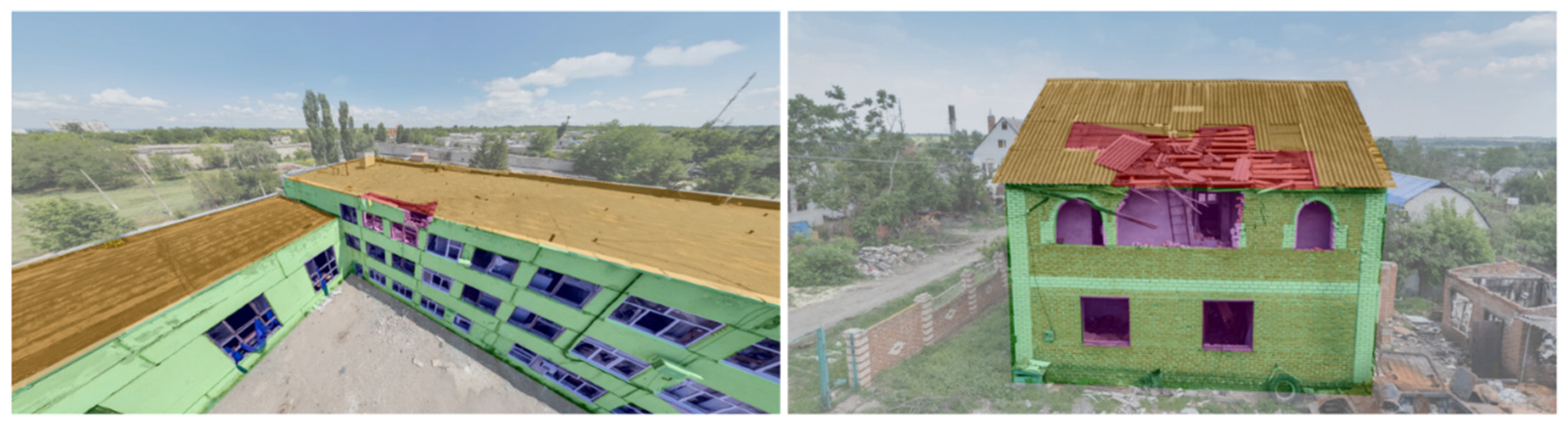
Figure 2.
Patch-based input representation. Each image is divided into fixed-size patches. A global image embedding is computed from the resized original image using ConvNeXt-Large. For each patch, its (x, y) position embedding is computed. The patch and its segmentation mask, along with global and positional embeddings, form a single dataset example.
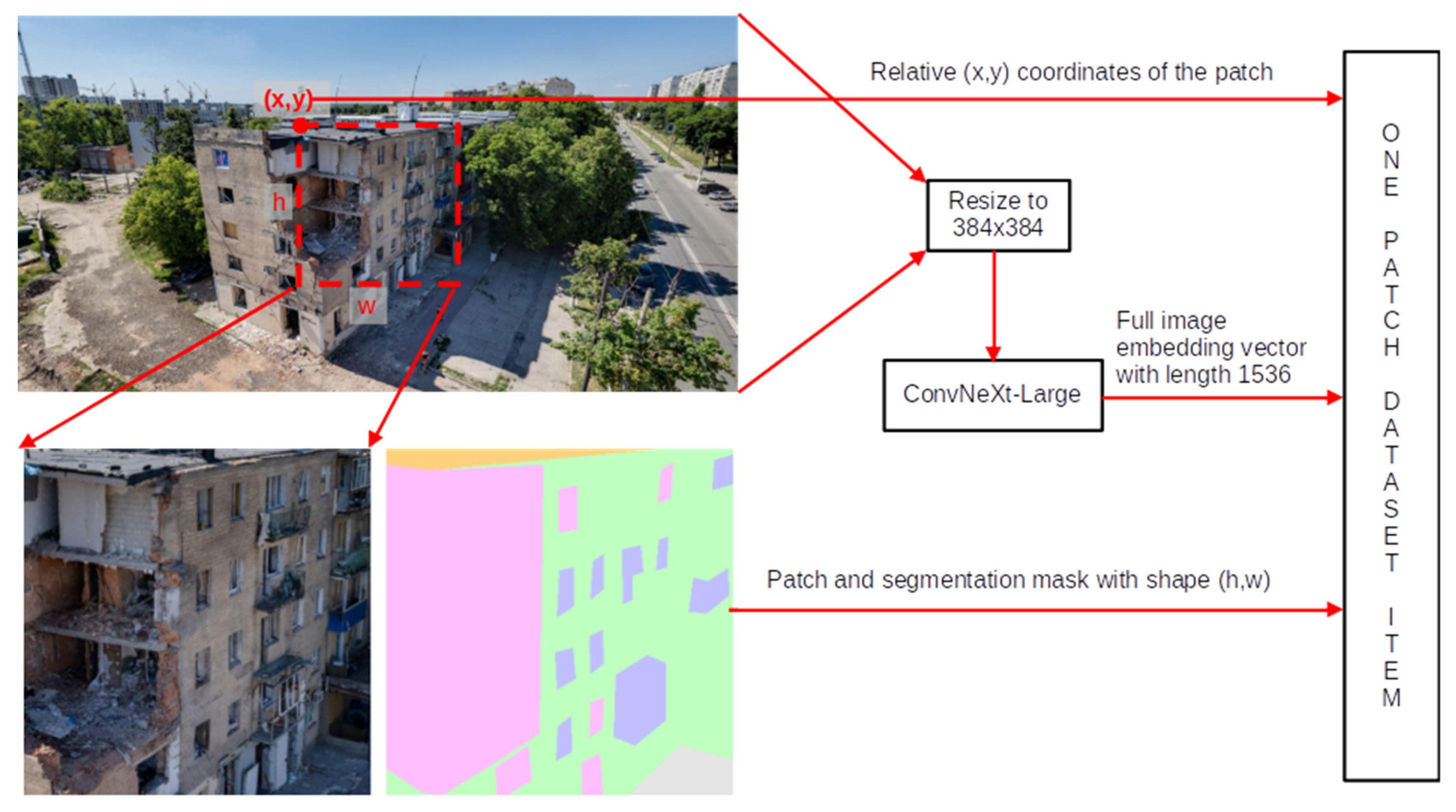
Figure 3.
Modified U-Net architecture with patch and embedding integration. The input patch passes through a single Encoder block. Skip connections feed features to each Decoder block. Encoder output is concatenated with the Global Embedding (ConvNeXt-Large) and the Positional Embedding before the Bottleneck. Decoder blocks use interpolation + convolution, and a final Conv2D layer outputs the segmentation mask.
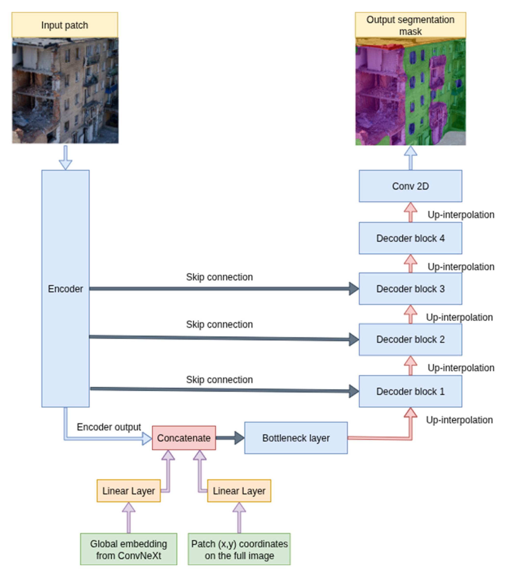
Figure 4.
Modified SegFormer architecture with patch and embedding integration. The input patch passes through a SegFormer model. Encoder output is concatenated with the Global Embedding (ConvNeXt-Large) and the Positional Embedding before the Bottleneck. Decoder blocks use interpolation + convolution, and a final Conv2D layer outputs the segmentation mask.
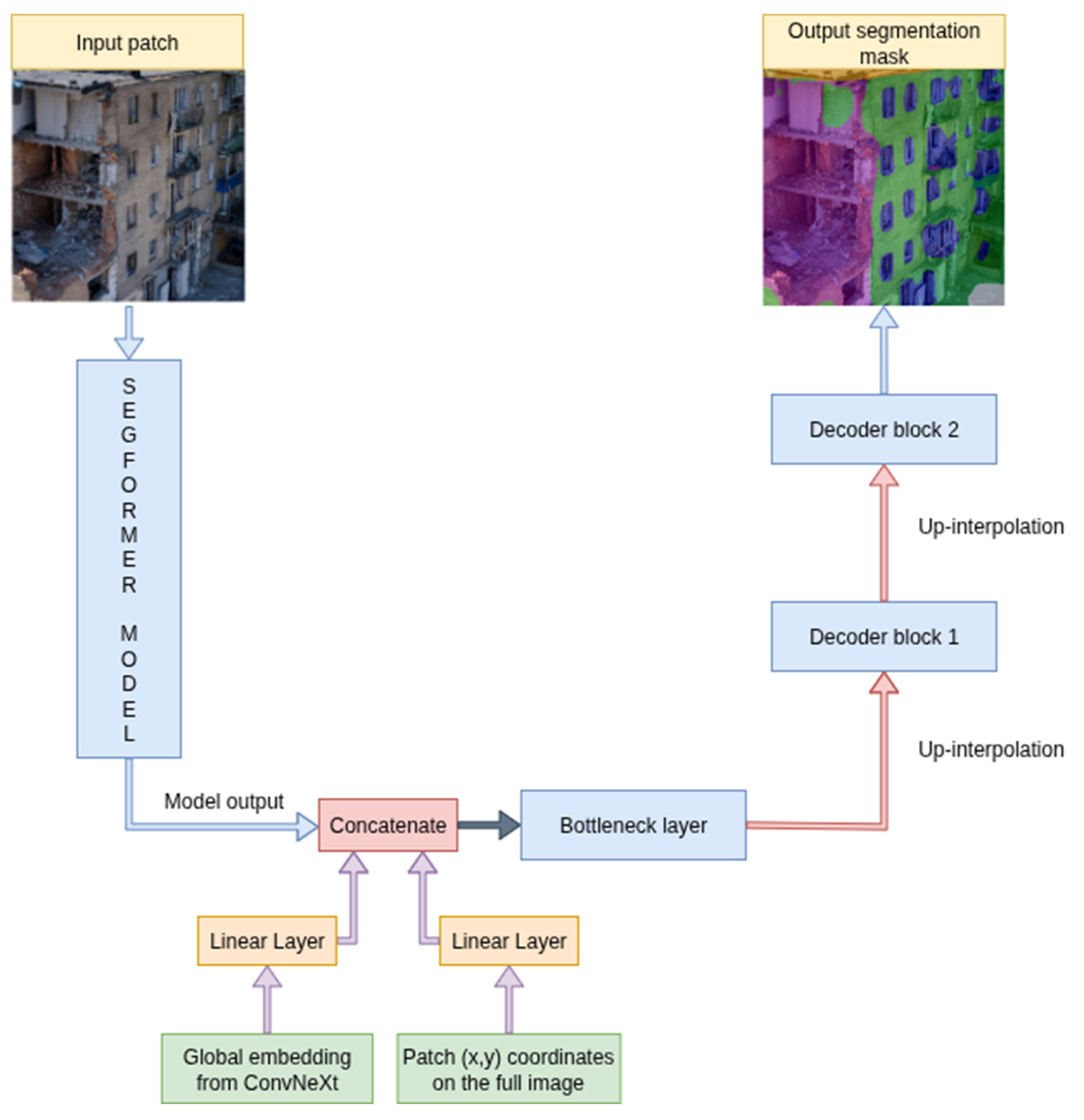
Figure 5.
Output of Felzenszwalb segmentation (scale = 300, sigma = 0.9, min_size = 50) on a damaged building image. Yellow contours mark regions grouped by local color and texture similarity.
Figure 5.
Output of Felzenszwalb segmentation (scale = 300, sigma = 0.9, min_size = 50) on a damaged building image. Yellow contours mark regions grouped by local color and texture similarity.
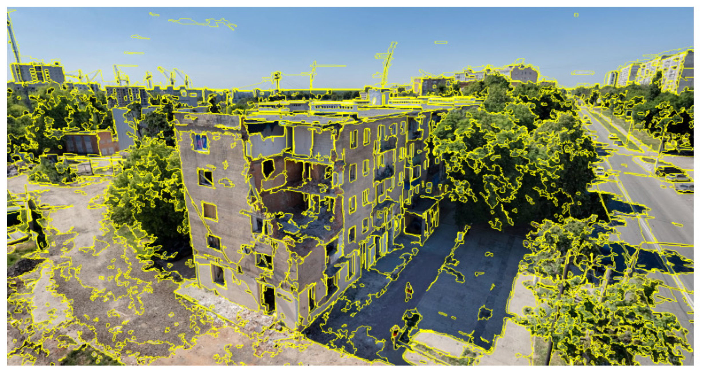
Figure 6.
Visual impact of embeddings on segmentation performance. Each row shows: first - original image, second - ground-truth segmentation mask, third - model prediction without embeddings, fourth - model prediction with embeddings. (a) Effect on ResNet in the 3-class setup. (b) Effect on ResNet in the 6-class setup. (c) Effect on DINOv2 in the 6-class setup. Color coding of classes: grey - Other, green - Building, purple - Damage, blue - Broken Window, orange - Roof, red - Damaged Roof.
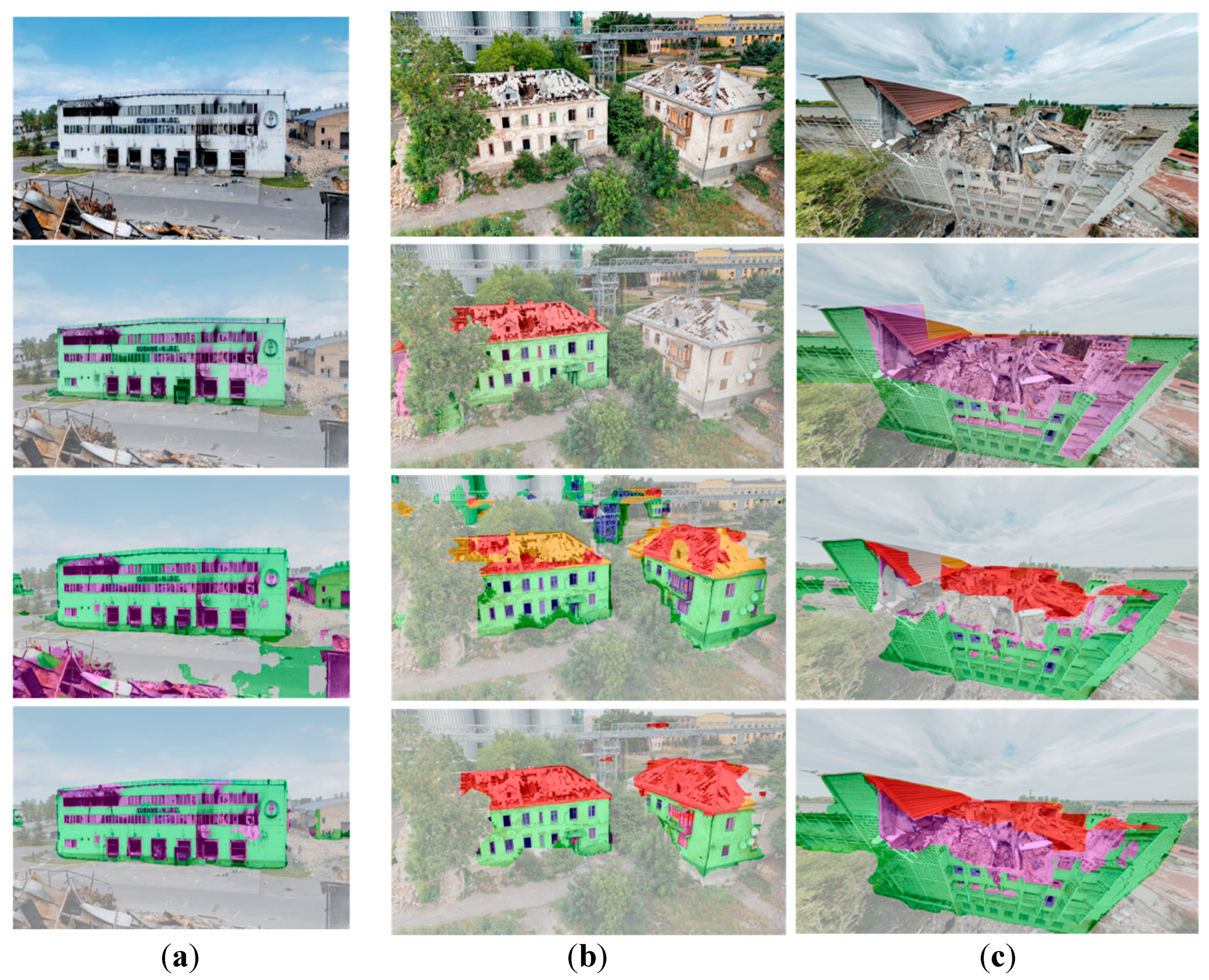
Figure 7.
Effect of superpixels on the DINOv2-Emb model in the 6-class setup. Top left - original image, bottom left - ground-truth segmentation mask, top right - DINOv2 with embeddings, bottom right - DINOv2 with embeddings and superpixels applied. Color coding of classes: grey - Other, green - Building, purple - Damage, blue - Broken Window, orange - Roof, red - Damaged Roof.
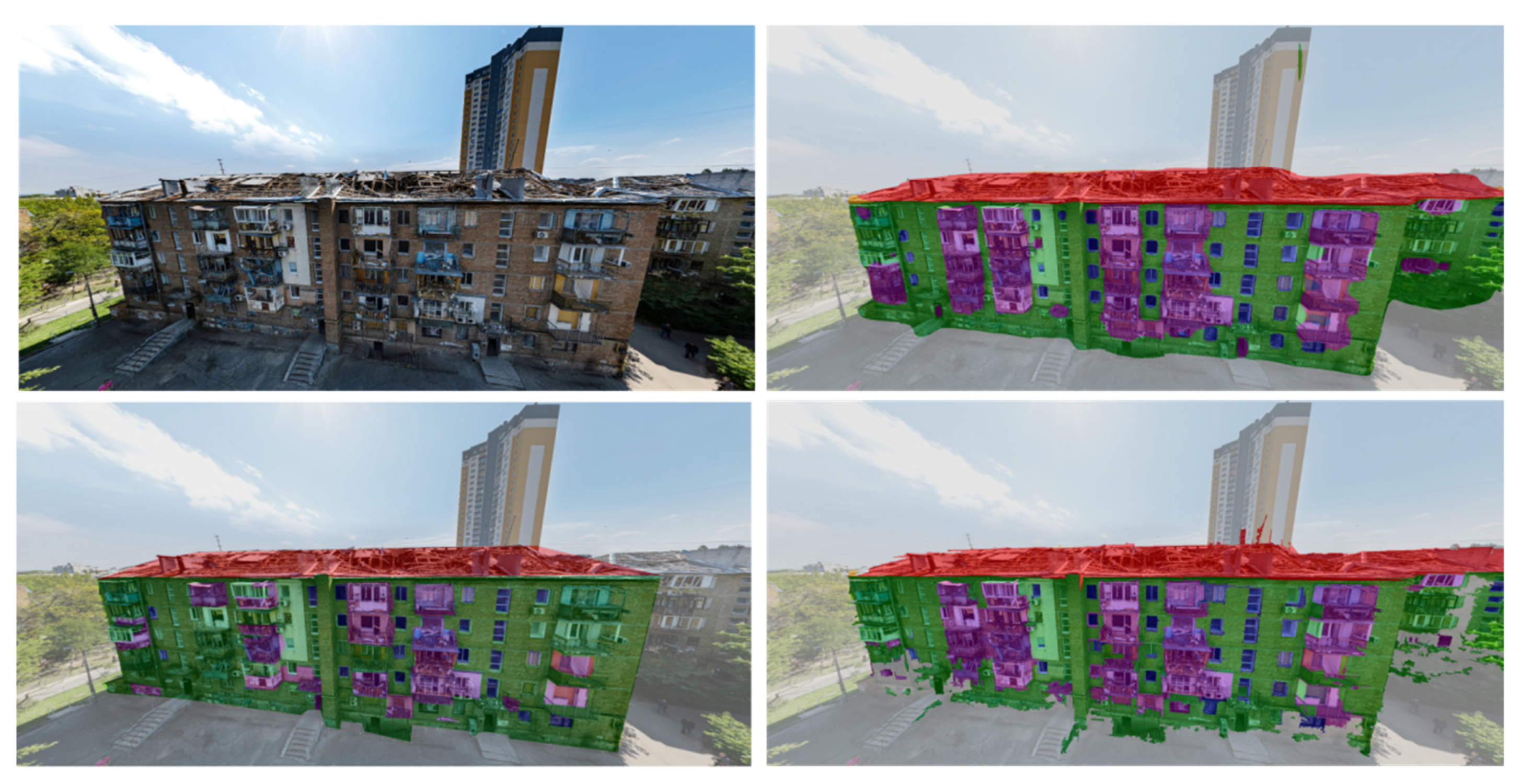
Table 1.
Class distribution in the dataset (percentages of total labeled pixels).
| Other | Building | Damage | Broken Window | Damaged Roof | Roof |
|---|---|---|---|---|---|
| 66.10% | 19.42% | 8.66% | 2.66% | 1.92% | 1.24% |
Table 2.
Patch-based dataset variants with resolution and sample counts. These variants are the same for the 3 and 6 class datasets.
Table 2.
Patch-based dataset variants with resolution and sample counts. These variants are the same for the 3 and 6 class datasets.
| Patch Size | Stride | Total Patches | Train Patches | Val Patches |
|---|---|---|---|---|
| 224×224 | 180 | 12,943 | 11,042 | 1,901 |
| 384×384 | 256 | 5,460 | 4,659 | 801 |
| 640×640 | 160 | 6,904 | 5,887 | 1,017 |
Table 3.
Architectural details of the encoders used in this study, including parameter counts, patch size and stride, skip connection layers, and the encoder output layer.
Table 3.
Architectural details of the encoders used in this study, including parameter counts, patch size and stride, skip connection layers, and the encoder output layer.
| Encoder | Parameters (M) | Patch Size/Stride | Skip Connection Layers | Encoder’s output layer |
|---|---|---|---|---|
| ResNet-50 | 23.5 | 224×224 / 180 | conv1, layer1, layer2, layer3 | layer4 |
| SwinV2 Large | 195.1 | 384×384 / 256 | Stages 1-3 outputs | Stage 4 |
| ConvNeXt-Large | 196.2 | 640×640 / 160 | Stages 1-3 outputs | Stage 4 |
| YOLO 11x-seg | 19.1 | 640×640 / 160 | Layers 1, 3, 5 | Layer 7 |
| DINOv2(ViT-L/14) | 266.5 | 640×640 1 / 160 | Blocks 1, 7, 12 | Block 20 |
1 For DINOv2, input patches were resized to 518×518 during data augmentations to match the model’s input constraints.
Table 5.
Learning rates and weight decays for each model.
| Model | Learning Rate | Weight Decay |
|---|---|---|
| ResNet | 3e-4 | 1e-2 |
| YOLO | 1e-4 | 1e-2 |
| Swin | 3e-5 | 1e-3 |
| ConvNeXT | 8e-6 | 1e-3 |
| DINOv2 | 2e-5 | 1e-3 |
| SegFormer | 2e-5 | 1e-3 |
Table 6.
Parameter counts (in millions) for each model, showing encoder, frozen encoder, decoder, and bottleneck contributions, as well as the total number of trainable parameters.
Table 6.
Parameter counts (in millions) for each model, showing encoder, frozen encoder, decoder, and bottleneck contributions, as well as the total number of trainable parameters.
| Model | Encoder | Freezed Encoder |
Decoder | Bottleneck | Total |
|---|---|---|---|---|---|
| ResNet50 | 23.5 | 0 | 12.5 | 34.6 | 70.6 |
| SwinV2 | 195.1 | 0.91 | 7 | 19.7 | 220.89 |
| ConvNeXt | 196.2 | 0 | 7 | 19.7 | 222.9 |
| SegFormer | 84.7 | 2.9 | 0.67 | 5.2 | 87.67 |
| YOLO | 19.1 | 0 | 4.3 | 7.5 | 30.9 |
| DINOv2 | 266.5 | 0 | 35.1 | 13.7 | 315.3 |
Table 7.
Average inference time per image (in seconds) for each model, measured with and without superpixel postprocessing.
Table 7.
Average inference time per image (in seconds) for each model, measured with and without superpixel postprocessing.
| Model | Without superpixels | With superpixels |
|---|---|---|
| ResNet50 | 4.41 | 9.55 |
| SwinV2 | 7.27 | 11.25 |
| ConvNeXt | 4.05 | 9.64 |
| SegFormer | 4.89 | 9.61 |
| YOLO | 4.32 | 8.82 |
| DINOv2 | 7.02 | 11.98 |
Table 8.
F1-scores for 3-class segmentation models across the categories: Other, Building, and Damage.
Table 8.
F1-scores for 3-class segmentation models across the categories: Other, Building, and Damage.
| Model | Other | Building | Damage | Mean |
|---|---|---|---|---|
| ResNet | 0.9489 | 0.8168 | 0.7704 | 0.8454 |
| ResNet-Emb | 0.9732 | 0.8721 | 0.8492 | 0.8982 |
| ResNet-Sup | 0.9437 | 0.8005 | 0.7464 | 0.8302 |
| ResNet-SupEmb | 0.9677 | 0.853 | 0.8192 | 0.88 |
| SwinV2 | 0,9317 | 0,7261 | 0,6929 | 0,7836 |
| SwinV2-Emb | 0,9451 | 0,7663 | 0,7166 | 0,8093 |
| SwinV2-Sup | 0.9308 | 0.7156 | 0.6838 | 0.7768 |
| SwinV2-SupEmb | 0.9434 | 0.7585 | 0.6961 | 0.7993 |
| ConvNeXt | 0.9365 | 0.7828 | 0.7225 | 0.8139 |
| ConvNeXt-Emb | 0.9472 | 0.7968 | 0.7336 | 0.8258 |
| ConvNeXt-Sup | 0.9399 | 0.7444 | 0.6717 | 0.7853 |
| ConvNeXt-SupEmb | 0.9557 | 0.78 | 0.6949 | 0.8102 |
| SegFormer | 0.9257 | 0.7753 | 0.6892 | 0.7967 |
| SegFormer-Emb | 0.9312 | 0.7776 | 0.6759 | 0.7949 |
| SegFormer-Sup | 0.9381 | 0.7612 | 0.6424 | 0.7805 |
| SegFormer-SupEmb | 0.936 | 0.7592 | 0.6364 | 0.7772 |
| YOLO11-seg | 0.9216 | 0.7335 | 0.6671 | 0.7741 |
| YOLO11-seg-Emb | 0.9487 | 0.7592 | 0.7132 | 0.807 |
| YOLO11-seg-Sup | 0.9242 | 0.7338 | 0.6571 | 0.7717 |
| YOLO11-seg-SupEmb | 0.9489 | 0.7545 | 0.6938 | 0.7991 |
| DINOv2 | 0.9625 | 0.8237 | 0.7821 | 0.8561 |
| DINOv2-Emb | 0.9593 | 0.8324 | 0.7855 | 0.859 |
| DINOv2-Sup | 0.9636 | 0.8031 | 0.7348 | 0.8339 |
| DINOv2-SupEmb | 0.9595 | 0.8016 | 0.7292 | 0.8301 |
Table 9.
F1-scores for 6-class segmentation models across the categories: Other, Building, Damage Broken Window, Damaged Roof, and Roof.
Table 9.
F1-scores for 6-class segmentation models across the categories: Other, Building, Damage Broken Window, Damaged Roof, and Roof.
| Model | Other | Building | Damage | Broken Window | Damaged Roof | Roof | Mean |
|---|---|---|---|---|---|---|---|
| ResNet | 0.9108 | 0.6897 | 0.5788 | 0.5315 | 0.3605 | 0.4472 | 0.5864 |
| ResNet-Emb | 0.9415 | 0.7168 | 0.6527 | 0.5192 | 0.5546 | 0.4744 | 0.6432 |
| ResNet-Sup | 0.9137 | 0.6866 | 0.582 | 0.5178 | 0.3608 | 0.4775 | 0.5897 |
| ResNet-SupEmb | 0.9412 | 0.7057 | 0.6439 | 0.5154 | 0.5431 | 0.4304 | 0.6299 |
| SwinV2 | 0.9313 | 0.7426 | 0.6477 | 0.5574 | 0.5131 | 0.4401 | 0.6387 |
| SwinV2-Emb | 0.9499 | 0.7537 | 0.6512 | 0.5516 | 0.6006 | 0.5512 | 0.6764 |
| SwinV2-Sup | 0.9327 | 0.7377 | 0.629 | 0.5472 | 0.5163 | 0.4404 | 0.6339 |
| SwinV2-SupEmb | 0.9503 | 0.7502 | 0.6328 | 0.541 | 0.6077 | 0.567 | 0.6748 |
| ConvNeXt | 0.9498 | 0.7467 | 0.628 | 0.496 | 0.5388 | 0.5814 | 0.6568 |
| ConvNeXt-Emb | 0.9448 | 0.7475 | 0.6219 | 0.5417 | 0.5781 | 0.5826 | 0.6694 |
| ConvNeXt-Sup | 0.9457 | 0.7328 | 0.6151 | 0.4819 | 0.5475 | 0.5945 | 0.6529 |
| ConvNeXt-SupEmb | 0.943 | 0.7427 | 0.6022 | 0.5271 | 0.5629 | 0.5775 | 0.6592 |
| SegFormer | 0.9342 | 0.7633 | 0.5713 | 0.525 | 0.4587 | 0.5189 | 0.6286 |
| SegFormer-Emb | 0.9355 | 0.7535 | 0.5061 | 0.5162 | 0.5239 | 0.592 | 0.6379 |
| SegFormer-Sup | 0.9335 | 0.7623 | 0.5625 | 0.5123 | 0.4611 | 0.5197 | 0.6252 |
| SegFormer-SupEmb | 0.9357 | 0.7504 | 0.501 | 0.4999 | 0.515 | 0.5785 | 0.6301 |
| YOLO11-seg | 0.9194 | 0.7262 | 0.5978 | 0.5236 | 0.4669 | 0.4359 | 0.6116 |
| YOLO11-seg-Emb | 0.9302 | 0.7039 | 0.6196 | 0.5161 | 0.534 | 0.5076 | 0.6352 |
| YOLO11-seg-Sup | 0.9226 | 0.7249 | 0.6014 | 0.5128 | 0.4646 | 0.478 | 0.6174 |
| YOLO11-seg-SupEmb | 0.9316 | 0.699 | 0.6116 | 0.5038 | 0.5447 | 0.5146 | 0.6342 |
| DINOv2 | 0.943 | 0.7985 | 0.5214 | 0.576 | 0.6647 | 0.6913 | 0.6991 |
| DINOv2-Emb | 0.9678 | 0.8057 | 0.7105 | 0.6063 | 0.703 | 0.684 | 0.7462 |
| DINOv2-Sup | 0.9451 | 0.7911 | 0.5539 | 0.5469 | 0.6606 | 0.6916 | 0.6982 |
| DINOv2-SupEmb | 0.9611 | 0.7859 | 0.6831 | 0.5723 | 0.6784 | 0.6685 | 0.7249 |
Table 10.
F1-score improvements from embeddings in 3-class segmentation models.
| Model | Other | Building | Damage | Mean |
|---|---|---|---|---|
| ResNet | 0.0243 | 0.0553 | 0.0788 | 0.0528 |
| SwinV2 | 0,0134 | 0,0402 | 0,0237 | 0,0257 |
| ConvNeXt | 0.0107 | 0.014 | 0.0111 | 0.0119 |
| SegFormer | 0.0055 | 0.0023 | -0.0133 | -0.0018 |
| YOLO11-seg | 0.0271 | 0.0257 | 0.0461 | 0.0329 |
| DINOv2 | -0.0032 | 0.0087 | 0.0034 | 0.0029 |
Table 11.
F1-score improvements from embeddings in 6-class segmentation models.
| Model | Other | Building | Damage | Broken Window | Damaged Roof | Roof | Mean |
|---|---|---|---|---|---|---|---|
| ResNet | 0.0307 | 0.0271 | 0.0739 | -0.0123 | 0.1941 | 0.0272 | 0.0568 |
| SwinV2 | 0.0186 | 0.0111 | 0.0035 | -0.0058 | 0.0875 | 0.1111 | 0.0377 |
| ConvNeXt | -0.005 | 0.0008 | -0.0061 | 0.0457 | 0.0393 | 0.0012 | 0.0126 |
| SegFormer | 0.0013 | -0.0098 | -0.0652 | -0.0088 | 0.0652 | 0.0731 | 0.0093 |
| YOLO11-seg | 0.0108 | -0.0223 | 0.0218 | -0.0075 | 0.0671 | 0.0717 | 0.0236 |
| DINOv2 | 0.0248 | 0.0072 | 0.1891 | 0.0303 | 0.0383 | -0.0073 | 0.0471 |
Table 12.
F1-score changes from superpixels in 3-class segmentation models, with the highest per-model improvement values highlighted in bold and the largest declines underlined.
Table 12.
F1-score changes from superpixels in 3-class segmentation models, with the highest per-model improvement values highlighted in bold and the largest declines underlined.
| Model | Other | Building | Damage | Mean |
|---|---|---|---|---|
| ResNet-Sup | -0.0052 | -0.0163 | -0.0240 | -0.0152 |
| ResNet-SupEmb | -0.0055 | -0.0191 | -0.0300 | -0.0182 |
| SwinV2-Sup | -0,0009 | -0,0105 | -0,0091 | -0,0068 |
| SwinV2-SupEmb | -0,0017 | -0,0078 | -0,0205 | -0,01 |
| ConvNeXt-Sup | 0.0034 | -0.0384 | -0.0508 | -0.0286 |
| ConvNeXt-SupEmb | 0.0085 | -0.0168 | -0.0387 | -0.0156 |
| SegFormer-Sup | 0.0124 | -0.0141 | -0.0468 | -0.0162 |
| SegFormer-SupEmb | 0.0048 | -0.0184 | -0.0395 | -0.0177 |
| YOLO11-seg-Sup | 0.0026 | 0.0003 | -0.0100 | -0.0024 |
| YOLO11-seg-SupEmb | 0.0002 | -0.0047 | -0.0194 | -0.0079 |
| DINOv2-Sup | 0.0011 | -0.0206 | -0.0473 | -0.0222 |
| DINOv2-SupEmb | 0.0002 | -0.0308 | -0.0563 | -0.0289 |
Table 13.
F1-score changes from superpixel post-processing in 6-class segmentation models, with the highest per-model improvement values highlighted in bold and the largest declines underlined.
Table 13.
F1-score changes from superpixel post-processing in 6-class segmentation models, with the highest per-model improvement values highlighted in bold and the largest declines underlined.
| Model | Other | Building | Damage | Broken Window | Damaged Roof | Roof | Mean |
|---|---|---|---|---|---|---|---|
| ResNet-Sup | 0.0029 | -0.0031 | 0.0032 | -0.0137 | 0.0003 | 0.0303 | 0.0033 |
| ResNet-SupEmb | -0.0003 | -0.0111 | -0.0088 | -0.0038 | -0.0115 | -0.044 | -0.0133 |
| SwinV2-Sup | 0.0014 | -0.0049 | -0.0187 | -0.0102 | 0.0032 | 0.0003 | -0.0048 |
| SwinV2-SupEmb | 0.0004 | -0.0035 | -0.0184 | -0.0106 | 0.0071 | 0.0158 | -0.0016 |
| ConvNeXt-Sup | -0.0041 | -0.0139 | -0.0129 | -0.0141 | 0.0087 | 0.0131 | -0.0039 |
| ConvNeXt-SupEmb | -0.0018 | -0.0048 | -0.0197 | -0.0146 | -0.0152 | -0.0051 | -0.0102 |
| SegFormer-Sup | -0.0007 | -0.001 | -0.0088 | -0.0127 | 0.0024 | 0.0008 | -0.0034 |
| SegFormer-SupEmb | 0.0002 | -0.0031 | -0.0051 | -0.0163 | -0.0089 | -0.0135 | -0.0078 |
| YOLO11-seg-Sup | 0.0032 | -0.0013 | 0.0036 | -0.0108 | -0.0023 | 0.0421 | 0.0058 |
| YOLO11-seg-SupEmb | 0.0014 | -0.0049 | -0.008 | -0.0123 | 0.0107 | 0.007 | -0.001 |
| DINOv2-Sup | 0.0021 | -0.0074 | 0.0325 | -0.0291 | -0.0041 | 0.0003 | -0.0009 |
| DINOv2-SupEmb | -0.0067 | -0.0198 | -0.0274 | -0.034 | -0.0246 | -0.0155 | -0.0213 |
Disclaimer/Publisher’s Note: The statements, opinions and data contained in all publications are solely those of the individual author(s) and contributor(s) and not of MDPI and/or the editor(s). MDPI and/or the editor(s) disclaim responsibility for any injury to people or property resulting from any ideas, methods, instructions or products referred to in the content. |
© 2026 by the authors. Licensee MDPI, Basel, Switzerland. This article is an open access article distributed under the terms and conditions of the Creative Commons Attribution (CC BY) license (http://creativecommons.org/licenses/by/4.0/).
Copyright: This open access article is published under a Creative Commons CC BY 4.0 license, which permit the free download, distribution, and reuse, provided that the author and preprint are cited in any reuse.


