
Submitted:
22 October 2025
Posted:
27 October 2025
You are already at the latest version
Abstract
Accurate estimation of actual evapotranspiration (ETa) is crucial for sustainable water management and efficient irrigation planning. This study presents a novel remote sensing data–driven one-step simulation–optimization framework designed for large-scale, multi-crop ETa estimation. Unlike conventional methods that rely on linear regression or iterative calibration for single crops, this framework simultaneously optimizes model parameters in a single step, capturing their nonlinear dynamics effectively. Daily ETa was estimated using remote sensing inputs, including NDVI, land surface temperature (LST), surface albedo (αs), alongside available meteorological data. The model was tested under two scenarios with different training and testing datasets. Scenario I, with limited data, achieved test R² = 0.8195 and all-data R² = 0.8152, closely matching Scenario II (test R² = 0.8357, all-data R² = 0.8162), demonstrating that high accuracy can be maintained even with reduced data availability. Optimal parameters were consistent across scenarios (a ≈ 0.315, b ≈ −0.0012), and seasonal performance remained stable. These results highlight the framework’s robustness, generalization capability, and practical applicability for ETa estimation in heterogeneous landscapes, emphasizing the power of remote sensing data–driven optimization.
Keywords:
actual evapotranspiration (ETa)
; remote sensing data
; one-step optimization framework
; multi-crop systems
; large-scale modeling
; water resource management
; simulation–optimization
1. Introduction
The estimation of actual evapotranspiration (ETa) is critically important for effective water resource management and agricultural irrigation planning. Accurate ETa prediction is essential for correctly characterizing the hydrological cycle and improving agricultural water management practices.
In recent years, several energy balance–based approaches have been developed to estimate crop water use and demand using remote sensing data. Prominent examples include SEBAL (Surface Energy Balance Algorithm for Land) [1], METRIC (Mapping Evapotranspiration at High Resolution with Internalized Calibration) [2], and SSEB (Simplified Surface Energy Balance) [3].
In addition to these models, Teixeira [4] proposed the Simple Algorithm for Evapotranspiration Retrieving (SAFER), a computationally efficient and biophysically realistic method designed for irrigated areas in semiarid regions. The SAFER algorithm estimates the evapotranspiration fraction (ETf = ETa/ETo) using remote sensing variables such as the normalized difference vegetation index (NDVI), spectral reflectance bands, land surface temperature, and basic meteorological inputs. By integrating vegetation and surface energy balance parameters with reference evapotranspiration (ETo) estimated through the Penman–Monteith method, SAFER enables accurate spatial mapping of surface evaporation [5–9].
The Penman–Monteith equation is widely recognized as the standard method for ETo estimation. However, its application is often limited by extensive data requirements, which has encouraged the development of alternative approaches that require fewer meteorological variables [10]. Among these, the Hargreaves–Samani method [11], which uses only maximum and minimum air temperature data, is frequently employed. Previous SAFER-based studies have primarily relied on ETo derived from the Penman–Monteith method [7,12], while applications utilizing simpler ETo estimation techniques remain scarce [6].
Given its data efficiency and biophysical grounding, the predictive performance of SAFER can be further enhanced through local calibration of its parameters, making it an effective tool for assessing surface evaporation over irrigated landscapes. Implementation of SAFER requires Landsat 8 reflectance data from the blue (B2), green (B3), red (B4), near-infrared (B5), and shortwave infrared (B6 and B7) bands, as well as radiance data from the thermal bands (B10 and B11). These inputs are essential for deriving surface albedo, brightness temperature, land surface temperature, and NDVI [13].
Numerous studies have demonstrated the successful application of SAFER for estimating ETa at daily and monthly scales. Representative examples include Nadeem et al. [14], Do Nascimento Leão et al. [15], and Venancio et al. [18], highlighting both the need for parameter recalibration and the challenge of transferring coefficients across regions with different climatic and cropping systems.
To address these limitations, Karahan et al. [19] developed an artificial neural network (ANN)–based model to estimate daily ETa using limited climatic and remote sensing data (NDVI, land surface temperature). Their approach combined satellite overpass data with minimal meteorological inputs to train the network, allowing daily ETa estimation without temporal interpolation. Evaluation across different data scenarios demonstrated high reliability (R² = 0.84).
2. Materials and Methods
2.1. Study Area and Data Used
The study area is located in the Lower Seyhan Plain (LSP), situated in the southeastern part of the Mediterranean Region of Türkiye (Figure 1). The site is approximately 30 km from the city center of Adana and covers an area of 9,495 hectares. The LSP represents a typical delta plain characterized by a highly flat topography with slopes of 1% or less, and an extensive irrigation and drainage network [19,20]. In this region, two cropping seasons are practiced each year—summer and winter—dominated mainly by citrus and other rotational crops [21].
Figure 1.
The study area is located in the southeastern Mediterranean region of Turkiye.
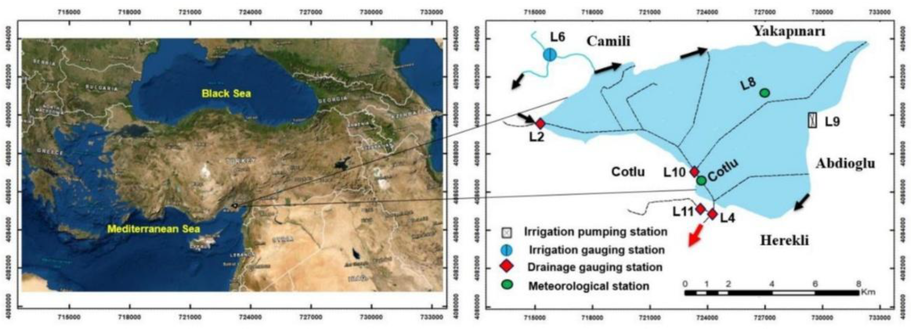
Meteorological data used in the study were obtained from the L8 and Cotlu meteorological stations located within the study area [19,21]. These data include daily measurements of minimum and maximum air temperature (Tmin, Tmax), wind speed (U), solar radiation (Rs), minimum and maximum relative humidity (RHmin, RHmax), and precipitation (P). The dataset covers 769 days of continuous observations between 16 September 2020 and 24 October 2022 [19]. Reference evapotranspiration (ETo, mm day⁻¹) was computed using the FAO-56 Penman–Monteith method [22].
According to Equation (1), the variables are defined as follows: ETo (mm day⁻¹) represents the reference evapotranspiration; Rn (MJ m⁻² day⁻¹) denotes the net radiation; G (MJ m⁻² day⁻¹) is the soil heat flux; (es − ea) indicates the vapor pressure deficit in the air (kPa); γ is the psychrometric constant (kPa °C⁻¹); Δ represents the slope of the saturation vapor pressure–temperature relationship (kPa °C⁻¹); u₂ (m s⁻¹) refers to the wind speed measured at a height of 2 m above the ground; and T (°C) is the mean air temperature, calculated as the average of the daily minimum and maximum temperatures
Satellite data required for actual evapotranspiration (ETa) estimation and METRIC model implementation were obtained from the United States Geological Survey (USGS) web platform (http://earthexplorer.usgs.gov) [2,23].
In addition, normalized difference vegetation index (NDVI) and land surface temperature (LST) parameters derived from the MODIS dataset were compiled via the Google Earth Engine (GEE) platform [24–26] and harmonized with the dataset used in Karahan et al. [19]. Using the same dataset ensures that the proposed model results can be directly compared with those of the ANN-based model presented by Karahan et al. [19].
To evaluate the linear relationships between independent variables (LST, albedo, NDVI, Rs, ETo) and the dependent variable (ETa), a Pearson correlation coefficient matrix was constructed, and the results are summarized in Figure 2.
Figure 2.
The correlation relationship between ETa and model parameters.
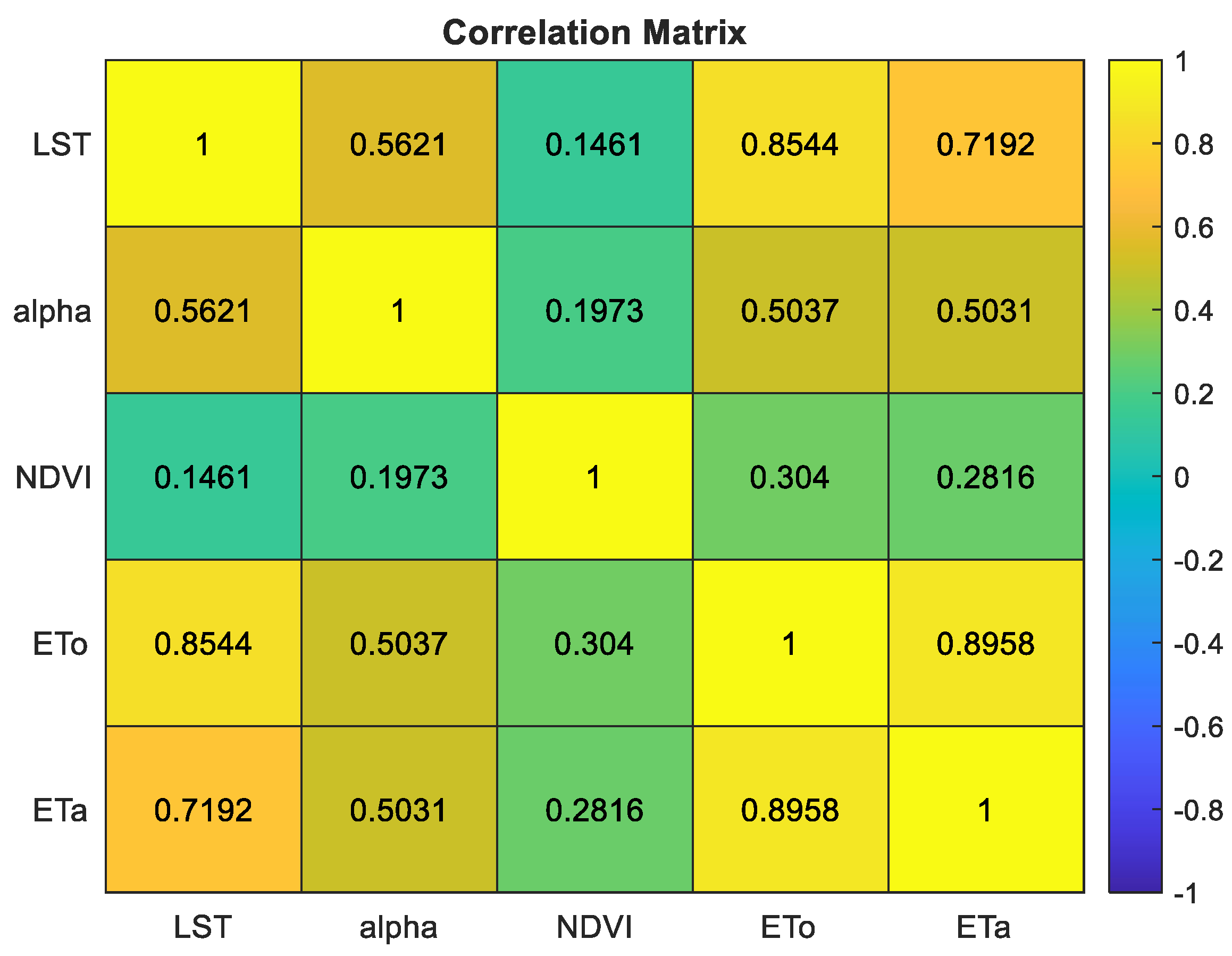
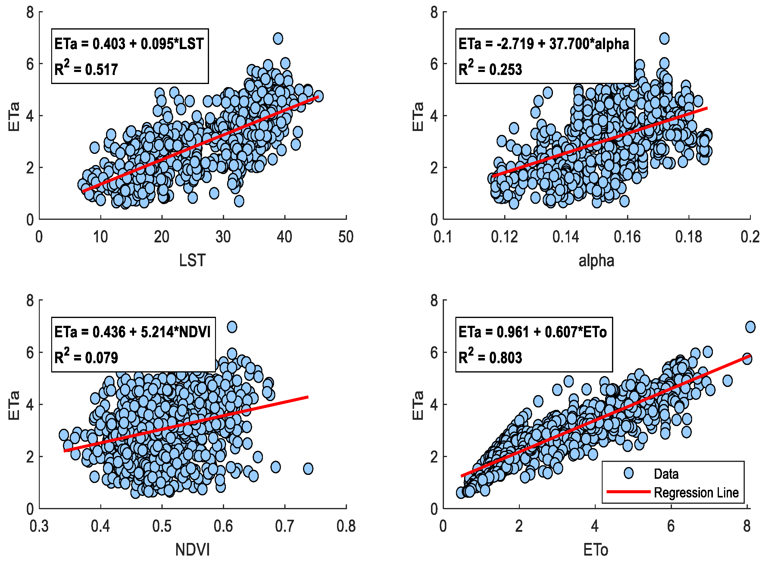
The correlation analysis revealed strong positive relationships between ETa and both ETo and Rs, while the correlations with LST, albedo, and NDVI were moderate to weak. This indicates that ETo and Rs should be considered as the primary predictors in ETa modeling, whereas the other variables contribute to improving the model performance and were therefore included as auxiliary inputs. Figure 3 illustrates the temporal variations of the model inputs and ETa values, while Figure 4 presents the correlation relationships between ETa and each variable. A joint evaluation of Figures 2, 3, and 4 clearly demonstrates a strong linear association between ETa and the investigated variables. Based on these findings, the model selection and design process are detailed in the following section.
Figure 3.
Temporal variation of the input variables used in the model.
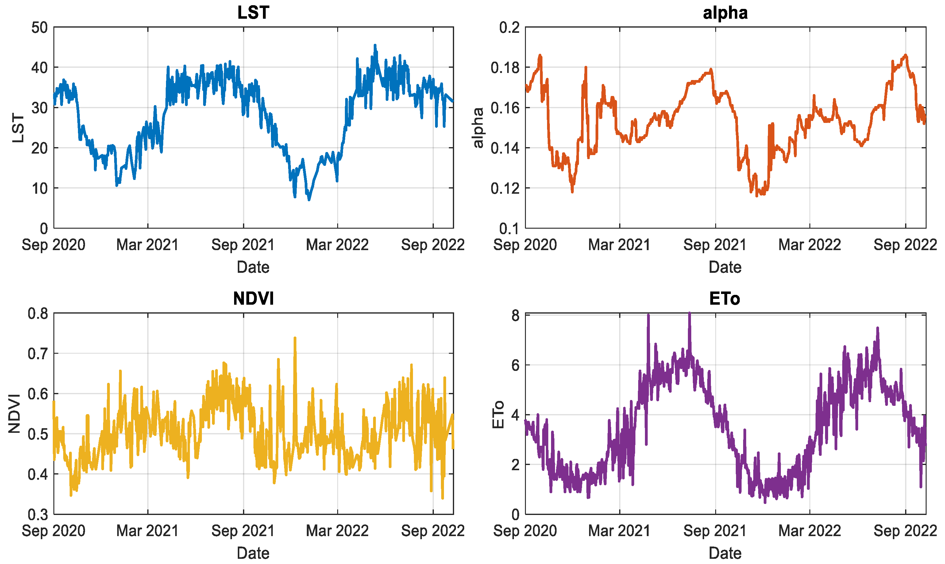
Figure 4.
Correlation relationships between ETa and the model input variables.
2.3. SAFER Model
The SAFER (Surface Energy Balance Algorithm for Evapotranspiration Retrieval) model is an energy balance-based approach that estimates actual evapotranspiration (ETa) using physical parameters derived from satellite imagery and meteorological data from ground stations [4,8]. Its main advantages include ease of implementation, applicability under extreme environmental conditions, no requirement for crop classification, and utilization of the ET/ETo ratio combined with remote sensing parameters [27]. The SAFER model was developed using field data from irrigated agricultural areas and the caatinga ecosystem in the semi-arid Middle-Lower São Francisco River Basin. It has been reported as an effective tool for ETa estimation in regions with limited data availability [6].
The model is expressed as follows:
Where a and b are regression (calibration) coefficients optimized according to site, sensor, or climatic conditions. T₀ represents the surface temperature obtained from thermal bands or other thermal indicators, while αₛ denotes the pixel surface albedo. ETa refers to the actual evapotranspiration (mm/day), and ETo represents the reference evapotranspiration (mm/day). In classical calibration, parameters are determined through linear regression using concurrent satellite data and field measurements (e.g., flux towers or lysimeters), ensuring region-specific calibration and enhancing model accuracy [7,18,28,29].
2.4. S/O-SAFER Optimization and SOS Algorithm
To improve the SAFER model’s performance, a heuristic-based Simulation-Optimization (S/O) approach was used to calibrate the a and b coefficients. Traditional linear regression methods, which assign fixed parameters via a single linear relationship, limit the model’s generalizability under varying climate and surface conditions.
Within the S/O framework, the Symbiotic Organisms Search (SOS) algorithm was employed. Developed by Cheng and Prayogo [30], SOS is a metaheuristic optimization inspired by symbiotic interactions among organisms. Each candidate solution improves through three types of interactions:
- Mutualism: In this interaction, both organisms benefit. New solutions are generated by combining the average of two organisms with the current best solution.
- Commensalism: In this interaction, one organism benefits while the other remains unaffected, leading to an improvement in the fitness of the benefiting organism.
- Parasitism: One organism attempts to improve by altering another’s solution; if superior, the new solution replaces the original.
These interaction mechanisms balance both the exploration and exploitation processes within the solution space, thereby increasing the likelihood of achieving a global optimum. The Symbiotic Organisms Search (SOS) algorithm has been applied in hydrology and water resources engineering, particularly in optimization problems such as flood routing and reservoir operation. In a study conducted on the Karun River, the parameters of the nonlinear Muskingum model were estimated using the SOS algorithm, and the results demonstrated lower error values compared to the Genetic Algorithm (GA) and Harmony Search (HS) methods [31] Similarly, in a study carried out on the Safarud Reservoir, the SOS algorithm was employed to determine the optimal reservoir operation strategy, and it was reported that the algorithm achieved fast convergence and high solution accuracy [32]. These studies indicate that the SOS algorithm is an effective optimization tool for the calibration of hydrological systems and for water resources management
The S/O-SAFER optimization proceeds in three phases:
- Initialization Phase: Random initial values for a and b are generated within predefined bounds.
- Prediction and Evaluation Phase: ETa is computed for each parameter combination using the SAFER model; predicted values are compared with measured data, and the Mean Squared Error (MSE) is calculated.
- Parameter Update Phase: SOS iteratively searches for the parameter combination that minimizes the error function, avoiding local minima and seeking a global optimum.
This approach allows local-scale optimization of SAFER parameters and enables reliable ETa estimation under different surface and climatic conditions.
2.5. Model Performance Evaluation
The S/O-SAFER model’s performance was evaluated by comparing daily measured ETa values with model predictions. The statistical indicators used included:
The model performance was evaluated using several statistical indicators, including the Mean Squared Error (MSE), Mean Absolute Error (MAE), Coefficient of Determination (R²), and Nash–Sutcliffe Efficiency (NSE). MSE quantifies the magnitude of prediction errors (mm/day), while MAE represents the mean absolute difference between predicted and observed values (mm/day). R² measures the proportion of variance explained by the model, and NSE assesses model performance in time series predictions [33].
During optimization, a and b parameters were determined using SOS, and ETa values were calculated for each combination. Tests under various data scenarios and meteorological conditions indicated that S/O-SAFER provides lower error metrics and higher correlation (R²) compared to classical SAFER.
The integration of satellite data (NDVI, surface temperature, albedo) with reference evapotranspiration (ETo) enhanced the model’s accuracy and allowed local adaptation of parameters for different crops and surface types. Overall, S/O-SAFER demonstrates superior performance in both optimization and predictive accuracy relative to conventional calibration methods.
3. Results
3.1. Application of the SAFER Model
The S/O-SAFER model produced daily ETa estimates by integrating NDVI, LST, ETo, Rs, and MODIS-derived surface albedo (αs) values. As illustrated in Figure 3, the model parameters exhibit notable temporal fluctuations, reflecting complex nonlinear dynamics that cannot be adequately captured using linear regression approaches. Therefore, a nonlinear simulation-optimization framework is essential to accurately capture parameter behavior and improve ETa prediction.
Derivative-based nonlinear optimization methods are sensitive to initial values and the search space, and they often risk becoming trapped in local minima [34,35]. To overcome these limitations, the Symbiotic Organisms Search (SOS) algorithm was applied, providing a robust, parameter-free, and globally balanced search capable of capturing the full nonlinear dynamics of the SAFER model parameters. Importantly, the SOS-based framework is flexible and can accommodate alternative heuristic algorithms, enhancing its general applicability.
The model was tested under two distinct scenarios to evaluate robustness and generalization: To assess the robustness and generalization capability of the proposed models, two experimental scenarios were established. In Scenario I, the dataset was partitioned such that 38 satellite overpass days were allocated for model training, while the remaining 731 days were used for independent testing. In Scenario II, 80% of the total 769-day dataset was randomly sampled for training, and the remaining 20% was reserved for model validation and testing.
3.1.1. Scenario I
For Scenario I, R² values of 0.7294 and 0.8195 and RMSE values of 0.6910 and 0.5694 were obtained for the training and testing phases, respectively, while for the entire dataset, R² = 0.8152 and RMSE = 0.5774 were achieved, as derived from the scatter plots shown in Figure 5. The P=O fit line and the regression lines nearly coincide, indicating excellent agreement between the observed and predicted ETa values
As shown in Figure 6, the seasonal variation in model performance is minimal, highlighting the model’s stability and high generalization capability across different temporal conditions.
3.1.2. Scenario II
In Scenario II, 80% of the dataset was used for training, resulting in optimal parameters of a = 0.311686 and b = −0.001216. For the complete dataset, R² = 0.8162 and RMSE = 0.5584 were obtained, as evidenced by the scatter distributions in Figure 7. The close overlap between the P = O reference line and the regression line demonstrates a strong consistency between the observed and predicted ETa values.
As depicted in Figure 8, the model maintains stable performance across different seasons, indicating its resilience and strong capacity to generalize under varying climatic conditions
3.2. Comparison of S/O-SAFER Performance with Alternative Models
Accurate calibration and evaluation of predictive models require benchmarking against established modeling and optimization approaches. In the context of ETa estimation, three widely used methods are:
Linear Regression (LR): LR models the relationship between dependent and independent variables assuming linearity [36]. It is simple, computationally efficient, and easy to interpret. However, its inability to capture nonlinear dynamics limits its predictive accuracy in heterogeneous, multi-crop landscapes.
Nelder-Mead (NM) Simplex Algorithm: NM is a derivative-free local search optimization method that adjusts parameters iteratively using a simplex of points to minimize an objective function [37]. NM can handle nonlinear optimization without requiring gradient information, but it is prone to convergence to local minima and may show unstable performance across datasets.
BFGS (Broyden–Fletcher–Goldfarb–Shanno) Algorithm: BFGS is a quasi-Newton optimization method that approximates the Hessian matrix to efficiently find the minimum of a smooth objective function [38]. While faster and often more accurate than NM, BFGS performance depends on initial parameter guesses and data quality, making it susceptible to noisy or sparse datasets.
3.2.1. Model Calibration and Performance Metrics
The S/O-SAFER model estimates daily actual evapotranspiration (ETa) using NDVI, land surface temperature (LST), and MODIS-derived surface albedo (αs) values, calibrated via a SOS-based one-step simulation–optimization framework. To evaluate the predictive performance, S/O-SAFER was benchmarked against LR, NM, and BFGS under two scenarios:
- Scenario I: Only limited satellite-observed days were used for training (38 days), with the remaining days for testing.
- Scenario II: Satellite-observed days combined with long-term field measurements were randomly split into 80% training and 20% testing sets.
Table 1 presents the optimal parameters (a, b) and performance metrics (MSE, MAE, RMSE, R²) for training, testing, and full datasets.
3.2.2. Comparative Performance Across Scenarios
The S/O-SAFER model consistently exhibits superior performance across both evaluation scenarios. In Scenario I, where the training data were limited, the model achieved a test value of 0.8195 and an all-data value of 0.8152, which are very close to the results obtained in Scenario II (test , all-data ). These outcomes indicate that the S/O-SAFER model maintains its predictive reliability even when trained with fewer data. In contrast, the linear regression model performed relatively poorly due to its inherent assumption of linearity, resulting in lower and higher RMSE values. The NM and BFGS optimization methods produced reasonably good results; however, they exhibited less stability and higher sensitivity to initial parameter settings and dataset characteristics compared to the S/O-SAFER model.
4. Discussion
Building on previous work, Karahan et al. (2024) applied an artificial neural network (ANN) to estimate evapotranspiration by integrating satellite-observed days with long-term field measurements. In that study, however, the ANN was trained using only approximately 5% of the total dataset, which was insufficient to fully capture the model’s peak performance. It was noted that increasing the number of measurements could overcome this limitation. In the present study, the S/O-SAFER model was developed using the same dataset as in the ANN study; however, the modeling approach and parameterization differ substantially, as S/O-SAFER relies on physically based inputs and a deterministic optimization structure rather than a purely data-driven algorithm.
As shown in Table 1, both scenarios yield nearly identical optimal parameter values (Scenario I: a = 0.3148, b = −0.0012; Scenario II: a = 0.3158, b = −0.0012). Despite the limited training dataset in Scenario I, its performance is remarkably close to that of Scenario II. Specifically, for the test set, Scenario I achieves R² = 0.8195 with RMSE = 0.5849, while Scenario II reaches R² = 0.8357 with RMSE = 0.5696. Across the full dataset, Scenario I attains R² = 0.8152 and RMSE = 0.5909, compared to Scenario II’s R² = 0.8162 and RMSE = 0.5943. These results indicate that Scenario I provides nearly equivalent performance to Scenario II, highlighting that high accuracy can be achieved without the additional effort and larger training set required in Scenario II.
The S/O-SAFER model estimates actual evapotranspiration (ETa) using NDVI, land surface temperature (LST), and daily surface albedo (αs). Across both scenarios, S/O-SAFER consistently outperforms conventional linear regression and alternative optimization approaches (Nelder–Mead and BFGS). While Nelder–Mead and BFGS occasionally achieve comparable results in certain subsets, their overall performance is less stable, further emphasizing S/O-SAFER’s robustness and generalization capability (Figure 5, Figure 6, Figure 7 and Figure 8).
Crucially, unlike previous studies focusing on small-scale plots or single crop types (e.g., maize or citrus), this study applies S/O-SAFER over a large, heterogeneous area with multiple cropping cycles per year. This spatial and temporal complexity considerably increases the challenge of accurately estimating ETa, making the model’s high performance particularly noteworthy. From both practical (covering diverse crop distributions and multiple harvests) and theoretical (stability and generalization over heterogeneous landscapes) perspectives, the study extends the utility of S/O-SAFER far beyond the scenarios reported in the literature.
Furthermore, in contrast to purely data-driven models such as ANNs, which may suffer from overfitting when data are limited, S/O-SAFER offers a deterministic, energy balance-based framework. Its physically interpretable structure provides reliable predictions with consistent seasonal performance, overcoming the fluctuations and inconsistencies inherent in black-box approaches. Notably, while ANN models also combine satellite-observed and long-term field measurements, their limited training subsets in previous studies prevented full performance realization, whereas S/O-SAFER achieves high accuracy using only NDVI, LST, αs, and available meteorological data—demonstrating the efficiency and practicality of Scenario I.
Overall, the results from Table 1 and Figure 5, Figure 6, Figure 7 and Figure 8 demonstrate that S/O-SAFER delivers superior accuracy, stability, and generalization across multiple scenarios, large-scale heterogeneous areas, diverse cropping patterns, and multi-harvest cycles. These findings establish S/O-SAFER as a robust, reliable, and highly applicable tool for sustainable water resource management and accurate crop evapotranspiration estimation.
5. Conclusions
The S/O-SAFER model, optimized through the SOS-based one-step simulation–optimization framework, effectively estimates daily actual evapotranspiration (ETa) using NDVI, LST, and MODIS-derived surface albedo (αs) across large, heterogeneous areas supporting both summer and winter crops. This study represents the first application of the S/O-SAFER model in a multi-crop, large-scale context, integrating parameter calibration and capturing nonlinear dynamics in a single optimization step, in contrast to previous approaches relying on linear regression or trial-and-error calibration for single crop types.
The optimum parameters obtained in both scenarios were highly consistent (Scenario I: a = 0.3148, b = −0.0012; Scenario II: a = 0.3158, b = −0.0012), and the model demonstrated robust performance. Scenario I achieved R² = 0.7294/0.8195 (training/testing) with RMSE = 0.6962/0.5849, while Scenario II achieved R² = 0.7310/0.8178 with RMSE = 0.6003/0.5696. For the full dataset, Scenario I attained R² = 0.8152 with RMSE = 0.5909, and Scenario II reached R² = 0.8162 with RMSE = 0.5943. The close alignment of parameter values and performance metrics across scenarios indicates that Scenario I, using a smaller training set, can achieve nearly the same accuracy as Scenario II, highlighting the efficiency and practicality of limited-data applications.
The similarity of the obtained parameters to those reported in previous studies [8] confirms the reliability of the S/O-SAFER framework under varying geographic and climatic conditions, while deviations from standard coefficients emphasize the necessity of regional and multi-crop calibration [19]. Unlike small-scale, single-crop studies, this work demonstrates that S/O-SAFER can accurately capture ETa dynamics over extensive areas with multiple crops and harvests per year, underscoring both its practical applicability and theoretical soundness.
Overall, the one-step, large-scale, multi-crop calibration framework provides a robust, reliable, and highly accurate tool for actual evapotranspiration estimation, suitable for regions with limited meteorological data, and capable of supporting improved water management and irrigation planning strategies. Scenario I, in particular, offers a nearly optimal balance between data requirements and model performance, demonstrating that high accuracy can be achieved without extensive field measurement efforts.
Acknowledgments
The author gratefully acknowledges the support of the Scientific and Technological Research Council of Turkey (TUBITAK) for project no. 122Y007, which provided the data used in this study.
Data Availability Statement
The data that support the findings of this study are available from the author upon reasonable request.
Conflicts of Interest
The author declares no conflict of interest.
Abbreviations
The following abbreviations are used in this
manuscript:
| S/O | Simulation/Optimization |
| SAFER | Simplified Approach for Evapotranspiration Retrieval |
| ETo | Reference Evapotranspiration |
| ETa | Actual Evapotranspiration |
| ETf | Evapotranspiration Fraction (ETa/ETo) |
| LST | Land Surface Temperature |
| NDVI | Normalized Difference Vegetation Index |
| α (alpha) | Surface Albedo Coefficient |
| SEBAL | Surface Energy Balance Algorithm for Land |
| METRIC | Mapping Evapotranspiration at High Resolution |
| SSEB | Simplified Surface Energy Balance |
| MODIS | Moderate Resolution Imaging Spectroradiometer |
| NM | Nelder–Mead Optimization Algorithm |
| BFGS | Broyden–Fletcher–Goldfarb–Shanno Optimization Algorithm |
| MSE | Mean Squared Error |
| MAE | Mean Absolute Error |
| RMSE | Root Mean Squared Error |
| R² | Coefficient of Determination |
References
- Bastiaanssen, W.G.M.; Pelgrum, H.; Wang, J.; Ma, Y.; Moreno, J.F.; Roerink, G.J.; van der Wal, T. A remote sensing surface energy balance algorithm for land (SEBAL). J. Hydrol. 1998, 212–213, 213–229. [Google Scholar] [CrossRef]
- Allen, R.G.; Tasumi, M.; Trezza, R. Satellite-Based Energy Balance for Mapping Evapotranspiration with Internalized Calibration (METRIC)—Model. J. Irrig. Drain. Eng. 2007, 133, 380–394. [Google Scholar] [CrossRef]
- Senay, G.B.; Bohms, S.; Singh, R.K.; Gowda, P.H.; Velpuri, N.M.; Alemu, H.; Verdin, J.P. Operational Evapotranspiration Mapping Using Remote Sensing and Weather Datasets: A New Parameterization for the SSEB Approach. JAWRA J. Am. Water Resour. Assoc. 2013, 49, 577–591. [Google Scholar] [CrossRef]
- de castro Teixeira, A.H. Determining Regional Actual Evapotranspiration of Irrigated Crops and Natural Vegetation in the São Francisco River Basin (Brazil) Using Remote Sensing and Penman-Monteith Equation. Remote. Sens. 2010, 2, 1287–1319. [Google Scholar] [CrossRef]
- Roerink, G.J.; Su, Z.; Menenti, M. S-SEBI: A simple remote sensing algorithm to estimate the surface energy balance. Phys. Chem. Earth Part B Hydrol. Oceans Atmos. 2000, 25, 147–157. [Google Scholar] [CrossRef]
- Santos, C.A.G.; de castro Teixeira, A.H.; da Silva, B.B.; da Cunha, A.C. Evapotranspiration mapping from Landsat-8 data by the SAFER algorithm in a tropical semi-arid region. Agric. Water Manag. 2020, 232, 106047. [Google Scholar]
- Coaguila, D.N.; Santos, C.A.G.; de castro Teixeira, A.H. Assessment of the SAFER model for estimating evapotranspiration in a tropical watershed. Remote Sens. Appl. Soc. Environ. 2017, 8, 88–98. [Google Scholar]
- de castro Teixeira, A.H.; Bastiaanssen, W.G.M.; Ahmad, M.D.; Bos, M.G. Reviewing SEBAL input parameters for assessing evapotranspiration and water productivity for the Brazilian semiarid region. Agric. For. Meteorol. 2013, 176, 39–50. [Google Scholar]
- de castro Teixeira, A.H.; Hernandez, F.B.T.; Lopes, H.L.; Scherer-Warren, M. Application of the SAFER model for mapping evapotranspiration in irrigated crops. Remote Sens. 2016, 8, 588. [Google Scholar]
- Ferreira, M.I.; Conceição, N.; Silva, J.M. Simplified approaches to estimate reference evapotranspiration in data-scarce regions. Agric. Water Manag. 2019, 217, 263–273. [Google Scholar]
- Hargreaves, G.H.; Samani, Z.A. Reference Crop Evapotranspiration from Temperature. Appl. Eng. Agric. 1985, 1, 96–99. [Google Scholar] [CrossRef]
- de castro Teixeira, A.H.; Leivas, J.F. Validation of the SAFER algorithm for evapotranspiration mapping in different Brazilian regions. Remote Sens. 2017, 9, 816. [Google Scholar]
- de castro Teixeira, A.H.; Coaguila, J.A.; Santos, C. Landsat 8 input data requirements for SAFER model application. Remote Sens. Appl. Soc. Environ. 2016, 4, 57–65. [Google Scholar]
- Nadeem, M.; Ahmad, M.U.D.; Ahmad, I. Groundwater depletion and evapotranspiration relationship using SAFER algorithm in Central Punjab, Pakistan. Environ. Monit. Assess. 2023, 195, 746. [Google Scholar]
- Do Nascimento Leão, M.; Santos, C.A.G.; de castro Teixeira, A.H. Estimation of evapotranspiration for citrus orchards using SAFER and Landsat imagery in the Brazilian Amazon. Remote Sens. Lett. 2025, 16, 1–12. [Google Scholar]
- de castro Teixeira, A.H. Regional evapotranspiration mapping in semiarid environments using remote sensing and surface energy balance models. Remote Sens. Environ. 2012, 123, 75–88. [Google Scholar]
- de castro Teixeira, A.H.; Bastiaanssen, W.G.M. Validation of the SAFER algorithm for evapotranspiration estimation under different conditions in Brazil. Remote Sens. Environ. 2013, 138, 50–63. [Google Scholar]
- Venancio, L.P.; de castro Teixeira, A.H.; Silva, B.B. Calibration and validation of SAFER model for maize evapotranspiration estimation in irrigated systems. Agric. Water Manag. 2021, 246, 106700. [Google Scholar]
- Karahan, H.; Cetin, M.; Can, M.E.; Alsenjar, O. Developing a New ANN Model to Estimate Daily Actual Evapotranspiration Using Limited Climatic Data and Remote Sensing Techniques for Sustainable Water Management. Sustainability 2024, 16, 2481. [Google Scholar] [CrossRef]
- Cetin, M.; Alsenjar, O.; Aksu, H.; Gölpınar, Y.; Akgül, M.A. Comparison of METRIC-based actual evapotranspiration estimates with in-situ water balance measurements over an irrigated field in Turkey. Hydrol. Sci. J. 2023, 68, 1162–1183. [Google Scholar] [CrossRef]
- Karahan, H.; Çetin, M.; Can, M.E.; Gültekin, U. TÜBİTAK (122Y007), Final Report; Tübitak: Ankara, Turkey, 2025. [Google Scholar]
- Allen, R.G.; Pereira, L.S.; Raes, D.; Smith, M. Crop Evapotranspiration: Guidelines for Computing Crop Water Requirements; FAO Irrigation and Drainage Paper No. 56; Food and Agriculture Organization of the United Nations: Rome, Italy, 1998. [Google Scholar]
- Tasumi, M.; Trezza, R.; Allen, R.G.; Wright, J.L. Operational aspects of satellite-based energy balance models for evapotranspiration mapping. Irrig. Drain. Syst. 2008, 22, 61–81. [Google Scholar]
- Didan, K. MOD13Q1 MODIS/Terra Vegetation İndices 16-day L3 Global 250 m SIN Grid V006; NASA EOSDIS Land Processes DAAC: Sioux Falls, SD, USA, 2015. [Google Scholar]
- Wan, Z.; Hook, S.; Hulley, G. MOD11A1 MODIS/Terra Land Surface Temperature/Emissivity Daily L3 Global 1 km SIN Grid V006; NASA EOSDIS Land Processes DAAC: Sioux Falls, SD, USA, 2015. [Google Scholar]
- Gorelick, N.; Hancher, M.; Dixon, M.; Ilyushchenko, S.; Thau, D.; Moore, R. Google Earth Engine: Planetary-scale geospatial analysis for everyone. Remote Sens. Environ. 2017, 202, 18–27. [Google Scholar] [CrossRef]
- de castro Teixeira, A.H.; Bastiaanssen, W.; Ahmad, M.D.; Moura, M.S.B.; Bos, M. Analysis of energy fluxes and vegetation-atmosphere parameters in irrigated and natural ecosystems of semi-arid Brazil. J. Hydrol. 2008, 362, 110–127. [Google Scholar] [CrossRef]
- Safre, A.L.S.; Nassar, A.; Torres-Rua, A.; Aboutalebi, M.; Saad, J.C.C.; Manzione, R.L.; de castro Teixeira, A.H.; Prueger, J.H.; McKee, L.G.; Alfieri, J.G.; et al. Performance of Sentinel-2 SAFER ET model for daily and seasonal estimation of grapevine water consumption. Irrig. Sci. 2022, 40, 635–654. [Google Scholar] [CrossRef]
- de castro Teixeira, A.H.; Leivas, J.; Takemura, C.; Garçon, E.; Sousa, I.; Azevedo, A. Monitoring anomalies on large-scale energy and water balance components by coupling remote sensing parameters and gridded weather data. Int. J. Biometeorol. 2024, 68, 2597–2612. [Google Scholar] [CrossRef]
- Cheng, M.-Y.; Prayogo, D. Symbiotic Organisms Search: A new metaheuristic optimization algorithm. Comput. Struct. 2014, 139, 98–112. [Google Scholar] [CrossRef]
- Khalifeh, H.; Choubin, B.; Moradi, E. Estimation of nonlinear parameters of the type 5 Muskingum model using the Symbiotic Organisms Search algorithm. Environ. Earth Sci. 2020, 79, 1–14. [Google Scholar]
- Rezaei-Estakhroueiyeh, H.; Ehteram, M.; Karami, H.; Kisi, O.; Singh, V.P. Data on optimal operation of Safarud Reservoir using Symbiotic Organisms Search (SOS) algorithm. Data Brief 2020, 30, 105548. [Google Scholar] [CrossRef]
- Nash, J.E.; Sutcliffe, J.V. River flow forecasting through conceptual models part I—A discussion of principles. J. Hydrol. 1970, 10, 282–290. [Google Scholar] [CrossRef]
- Karahan, H. Discussion of “Parameter Estimation of Nonlinear Muskingum Models Using Nelder-Mead Simplex Algorithm” by Reza Barati. J. Hydrol. Eng. 2013, 18, 365–367. [Google Scholar] [CrossRef]
- Karahan, H. Discussion of the “Enhanced Nonlinear Muskingum Model with Variable Exponent Parameter” by M. Easa. J. Hydrol. Eng. 2014, 19, 07014007. [Google Scholar] [CrossRef]
- Montgomery, D.C.; Peck, E.A.; Vining, G.G. Introduction to Linear Regression Analysis; John Wiley & Sons: Hoboken, NJ, USA, 2021. [Google Scholar]
- Nelder, J.A.; Mead, R. A Simplex Method for Function Minimization. Comput. J. 1965, 7, 308–313. [Google Scholar] [CrossRef]
- Nocedal, J.; Wright, S.J. Numerical Optimization, 2nd ed.; Springer: New York, NY, USA, 2006. [Google Scholar]
Figure 5.
Comparison between observed and predicted ETa values for training, test, and full datasets (Scenario I).
Figure 5.
Comparison between observed and predicted ETa values for training, test, and full datasets (Scenario I).
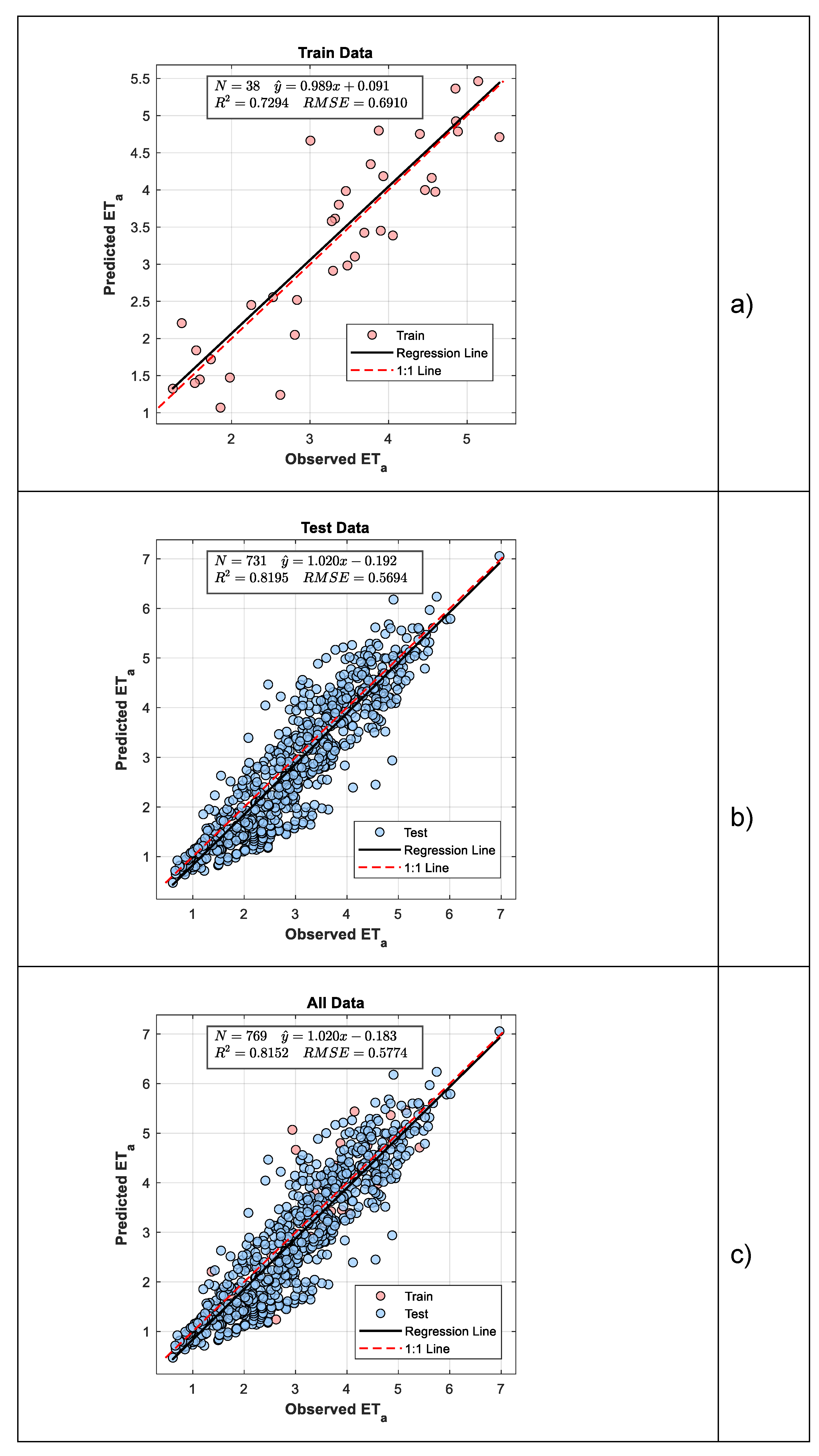
Figure 6.
Temporal variation of model results for Scenario I, illustrating the seasonal stability and general agreement of predicted ETa with observations.
Figure 6.
Temporal variation of model results for Scenario I, illustrating the seasonal stability and general agreement of predicted ETa with observations.
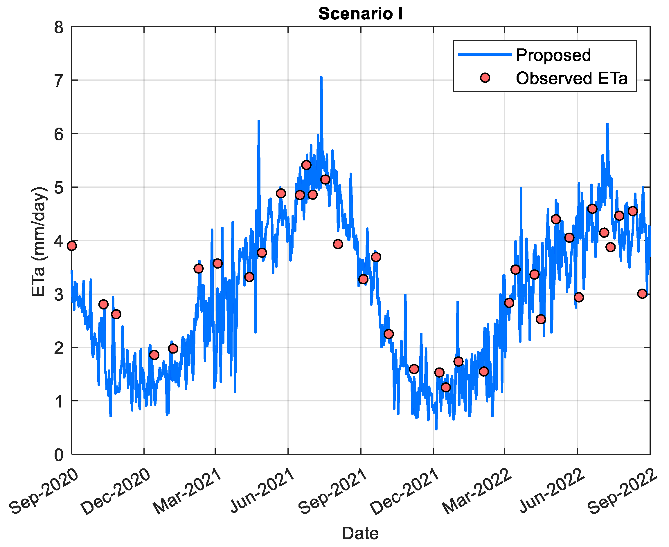
Figure 7.
Model results for Scenario II, showing the comparison between observed and predicted ETa values for training, test, and full datasets.
Figure 7.
Model results for Scenario II, showing the comparison between observed and predicted ETa values for training, test, and full datasets.
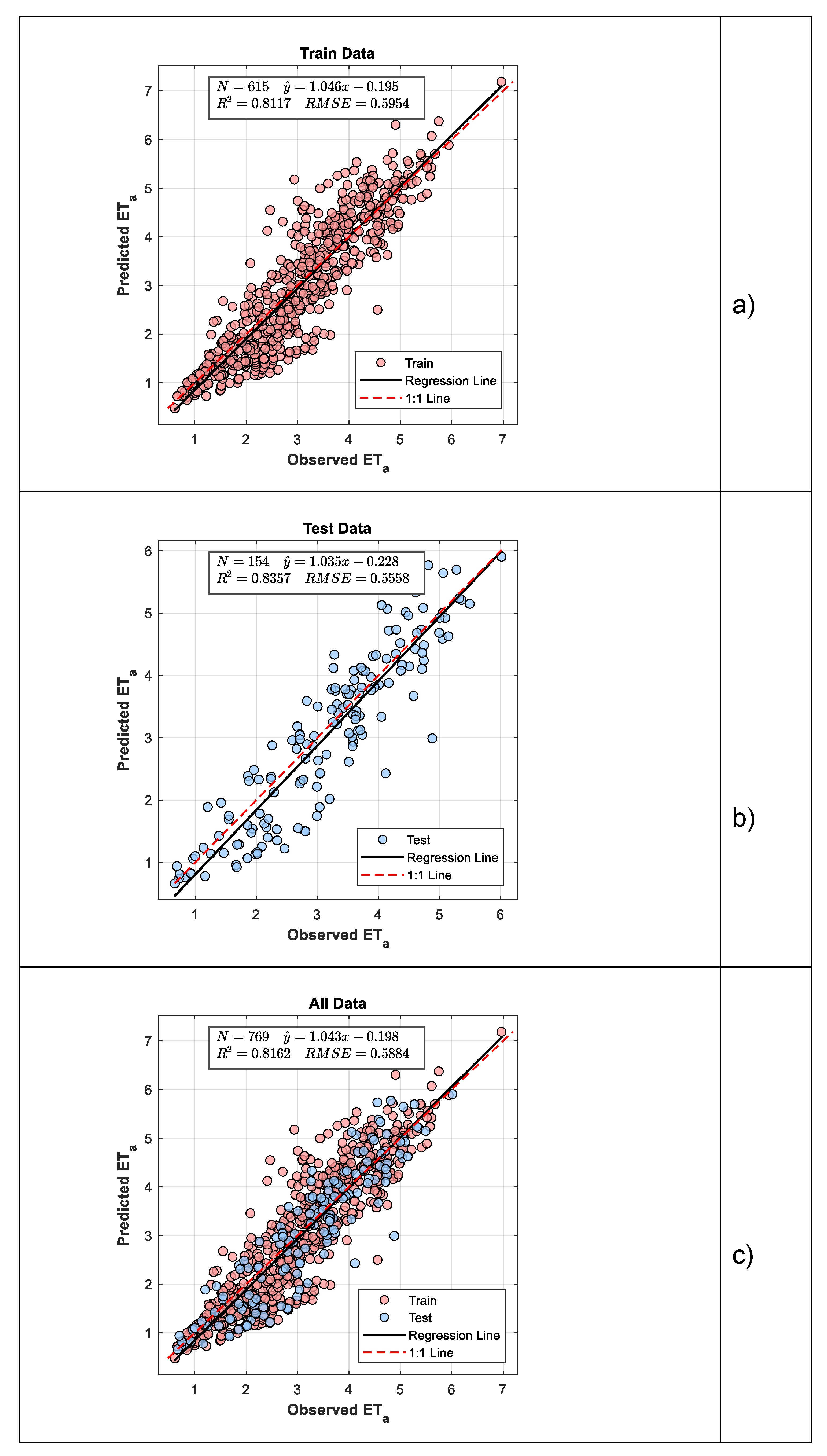
Figure 8.
Temporal variation of model results for Scenario II, demonstrating the consistent alignment of predicted and observed ETa values throughout the study period.
Figure 8.
Temporal variation of model results for Scenario II, demonstrating the consistent alignment of predicted and observed ETa values throughout the study period.
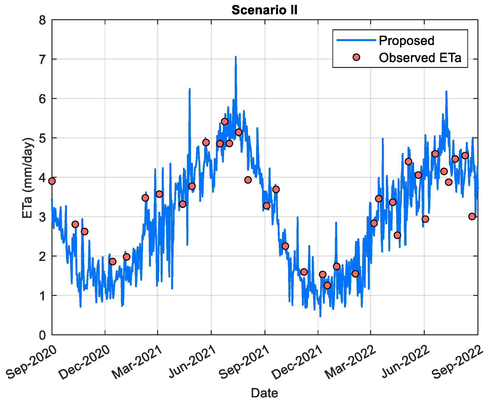

Table 1.
Performance metrics of S/O-SAFER, Linear Regression, Nelder-Mead, and BFGS models for Scenario I and II.
Table 1.
Performance metrics of S/O-SAFER, Linear Regression, Nelder-Mead, and BFGS models for Scenario I and II.
| Model | Scenario | Model Parameters | Dataset | MSE | MAE | RMSE | R2 | |
|---|---|---|---|---|---|---|---|---|
| a | b | |||||||
| S/O SAFER | I | 0.3148 | -0.0012 | Training | 0.4848 | 0.5312 | 0.6962 | 0.7294 |
| Testing | 0.3421 | 0.4548 | 0.5849 | 0.8195 | ||||
| All Data | 0.3492 | 0.4586 | 0.5909 | 0.8152 | ||||
| II | 0.3158 | -0.0012 | Training | 0.3604 | 0.4652 | 0.6003 | 0.8117 | |
| Testing | 0.3245 | 0.4479 | 0.5696 | 0.8357 | ||||
| All Data | 0.3532 | 0.4617 | 0.5943 | 0.8162 | ||||
| Linear Reg. | I | 0.4395 | -0.0014 | Training | 0.3732 | 0.4778 | 0.6109 | 0.7342 |
| Testing | 0.4184 | 0.5130 | 0.6468 | 0.7076 | ||||
| All Data | 0.3868 | 0.4884 | 0.6219 | 0.7265 | ||||
| Nelder-Mead | 0.2927 | -0.0012 | Training | 0.3310 | 0.4440 | 0.5753 | 0.7643 | |
| Testing | 0.3919 | 0.4893 | 0.6260 | 0.7261 | ||||
| All Data | 0.3493 | 0.4576 | 0.5910 | 0.7530 | ||||
| BFGS | 0.4145 | -0.0015 | Training | 0.3382 | 0.4549 | 0.5815 | 0.7591 | |
| Testing | 0.3919 | 0.4970 | 0.6260 | 0.7261 | ||||
| All Data | 0.3543 | 0.4675 | 0.5953 | 0.7494 | ||||
Disclaimer/Publisher’s Note: The statements, opinions and data contained in all publications are solely those of the individual author(s) and contributor(s) and not of MDPI and/or the editor(s). MDPI and/or the editor(s) disclaim responsibility for any injury to people or property resulting from any ideas, methods, instructions or products referred to in the content. |
© 2025 by the author. Licensee MDPI, Basel, Switzerland. This article is an open access article distributed under the terms and conditions of the Creative Commons Attribution (CC BY) license (https://creativecommons.org/licenses/by/4.0/).
Copyright: This open access article is published under a Creative Commons CC BY 4.0 license, which permit the free download, distribution, and reuse, provided that the author and preprint are cited in any reuse.


